Late-Type Dwarf Galaxies in the Virgo Cluster: II. Star Formation Properties

Abstract

We study star-formation-inducing mechanisms in galaxies through multi-wavelength measurements of a sample of dwarf galaxies in the Virgo cluster described in paper I. Our main goal is to test how star formation inducing mechanisms depend on several parameters of the galaxies, such as morphological type and hydrogen content. We derive the star formation rate and star formation histories of the galaxies, and check their dependence on other parameters.

Comparison of the sample galaxies with population synthesis models shows that these objects have significantly lower metallicity than the Solar value. The colors can generally be explained as a combination of two different stellar populations: a young (3–20 Myr) metal-poor population which represents the stars currently forming presumably in a starburst, and an older (0.1–1 Gyr) population of previous stellar generations. There is evidence that the older stellar population was also formed in a starburst. This is consistent with the explanation that star formation in this type of objects takes place in short bursts followed by long quiescent periods.

No significant correlation is found between the star formation properties of the sample galaxies and their hydrogen content. Apparently, when star formation occurs in bursts, other parameters influence the star formation properties more significantly than the amount of atomic hydrogen. No correlation is found between the projected Virgocentric distance and the rate of star formation in the galaxies, suggesting that tidal interactions are not significant in triggering star formation in cluster dwarf galaxies.

Key words: Galaxies, star-formation; Galaxies, evolution; Galaxies, individual

1 Introduction

Star formation is probably the most fundamental process in galaxies. Understanding its nature, and its dependence on galactic type and environment may contribute to our knowledge about development of galaxies, as well as about the development of the entire Universe.

The star formation process is characterized by two main parameters: the initial mass function (IMF) and the total star formation rate (SFR). First introduced by Salpeter (1955), the IMF is usually described as a power law in the range of 2–2.5 (the original value proposed by Salpeter is 2.35). Other characteristics of the IMF are the low and high mass limits, usually taken as 0.1M_⊙ and 60–120M_⊙. Several typical IMFs describe star formation in different types of galaxies and environments, such as the solar neighborhood, the Magellanic clouds, etc. Some IMFs (e.g, Miller and Scalo 1979, and Scalo 1986) were not published originally as power laws, but can be fitted as power laws with varying coefficients for different mass ranges. In Fig. 1 four different IMFs, used in various models, are shown.

Figure 1: Different IMFs by several authors. The power law coefficients are indicated close to each segment of the relations. The tick marks on the abscissa are one unit apart, i.e., each tick mark corresponds to a factor of 10 in the number of stars formed per unit mass. The designations are as follows: S55 $\equiv$ Salpeter (1955), K83 $\equiv$ Kennicutt (1983), MS97 $\equiv$ Miller & Scalo (1979), S86 $\equiv$ Scalo (1986). The MS79 and S86 IMFs are shown as parameterized by Bruzual & Charlot (1993).

As for the SFR, its time dependence varies dramatically between different galactic types (e.g., Gallagher, Hunter & Tutukov 1984; Kennicutt et al. 1994). In early type galaxies, the star formation usually decays smoothly with time. In late-type galaxies, on the other hand, the star formation is generally more intense, and the SFR is subject to significant changes on short timescales.

Despite extensive progress in understanding the star formation process, there are several issues still not fully understood. In paper I we introduced two open questions concerning the star formation processes in galaxies: (1) What are the mechanisms that govern the star formation process, and how do they depend on the galactic type and environment? (2) How do the SFR and IMF depend on various galactic properties, such as interstellar gas density, morphology of the interstellar gas, metallicity and the amount of dust in the interstellar medium.

The simplified assumption is that the SFR depends directly on the density of the interstellar gas (Schmidt law, Schmidt 1959). Actually, the observable quantity is the gas surface density. Testing this parameter against the SFR in normal galaxies indicates that there is a threshold gas surface density, below which no star formation takes place (Kennicutt 1989). The value of this threshold surface density varies from galaxy to galaxy, thus it is not a global parameter, though it is believed to be of order a few times $10^{20}atoms/cm^{2}$.

Larson (1987) counts four major mechanisms that induce star formation in galaxies: large scale gravitational instabilities of gas clouds, compression of interstellar gas clouds due to the passage of a gravitational density wave, compression in a rotating galactic disk - shear forces acting on the clouds due to differential rotation and random collisions between clouds. In addition, star formation can be triggered by external influences, such as tidal interaction induced by another galaxy during a close encounter of two galaxies, or by interaction with interstellar matter, during a passage near a cluster core.

In order to investigate the above questions, we have constructed four samples of galaxies, described in paper I. These galaxies are all dwarfs in the Virgo cluster. The aim in selecting dwarf galaxies is to eliminate some of the mechanisms described above, i.e. the grand design density wave and shear differential rotation forces do not act in dwarf galaxies. Therefore the theoretical situation is simplified.

Our goal in this paper is to derive the star formation properties of the sample galaxies from the observational data gathered in paper I, and to check these againts various star formation scenarios. This will enable to test the feasibility of several star formation mechanisms.

Since all methods used to determine galactic star formation properties combine observational data with theoretical models, the result is model dependent. Realistic models which use conventional IMFs and reliable stellar evolutionary tracks would result in SFR values that may differ usually by at most $\sim$50% from each other, given the same observational data. This is approximately the accuracy of our observed parameters from which the SFR is derived. As will be discussed below, the uncertainty is mainly due to effects of dust extinction and other observational biases.

In order to estimate the SFR in a sample of galaxies, one needs to know the IMF. This can be found by fitting a number of observed properties to a set of models of different stellar populations, with different IMFs (population synthesis). Since the colors of a stellar population depend also on its age and history, a specific star formation history is usually assumed, and the observed properties can be tested against different IMFs. Naturally, this approach can be used only for entire samples of galaxies and not for individual galaxies.

Once the IMF is determined (or assumed), the SFR can be calculated on the basis of models + observations. All the observational techniques basically measure the number of massive stars in the galaxy to trace the ’current’ star formation. If the lifetime of stars with a certain mass $M$ is $T(\!M\!)$ and the star formation rate at this mass is $R(\!M\!)$, then the number of such stars currently observed is simply $N(\!M\!)=R(\!M\!)\times T(\!M\!)$, where both $R(\!M\!)$ and $N(\!M\!)$ are given per unit stellar mass.

The total SFR is calculated by extrapolating from the massive stars to the entire mass range, using the IMF. The higher the mass of the stars we use, the larger the error of the total SFR that can be introduced due to the extrapolation. On the other hand, concentrating on higher mass stars leads to a more ’up to date’ star formation result. Therefore, there is a tradeoff between how ‘current’ the derived SFR is, and the accuracy of the total SFR. In paper I we described the observations of UV and H$\alpha$ line radiation from the sample galaxies, which we use here for determination of their SFR.

The relation between the number of observed LyC photons and the SFR can be reduced to the knowledge of the dependence of $R(\!M\!)$ on $M$, and the number of LyC photons emitted by a star with mass $M$ during its entire lifetime $P(\!M\!)$. With these two parameters, the number of photons emitted per unit time by an $M$ mass star (per unit stellar mass) is $F(\!M\!)=P(\!M\!)\times R(\!M\!)$, and the total flux of LyC photons is given by:

$$N_{c}=\int_{M_{min}}^{M_{max}}F(\!M\!)\;dM=\int_{M_{min}}^{M_{max}}P(\!M\!)\cdot R(\!M\!)\;dM$$ (1)

where $M_{min}$ and $M_{max}$ are the low and high mass limits of the IMF, and the dependence of $R(\!M\!)$ on $M$ is the IMF.

We can now express the number of LyC photons as:

$$N_{c}=S\!F\!R\;\frac{{\displaystyle\int_{M_{min}}^{M_{max}}P(\!M\!)\cdot I\!M\!F(\!M\!)\;dM}}{{\displaystyle\int_{M_{min}}^{M_{max}}M\cdot I\!M\!F(\!M\!)\;dM}}$$ (2)

where $S\!F\!R$ is in M_⊙/yr, and the integrals in the equation originate from the theoretical models. We therefore obtain a direct relation between the SFR and the number of LyC photons.

This treatment assumes a constant IMF. However, some studies indicate a dependence of the IMF on the metallicity of the galaxy (e.g., Terlevich & Melnick 1983). The metallicity of a galaxy gradually increase wirh time, thus, the IMF will also depend on the galactic age. In this case the SFR and IMF would be coupled and will be changing in time.

The LyC flux is derived here through its influence on the ambient hydrogen, e.g., by measurement of the resulting Balmer lines and assuming case B recombination. For the calculation of the SFR we use the H$\alpha$ line. This line has been used by many (Kennicutt 1983, hereafter K83, Kennicutt & Kent 1983; Gallagher, Hunter & Tutukov 1984; Pogge and Eskridge 1987; Kennicutt et al. 1994), mainly because of its high intensity. A few percent of the total ionizing flux are reemitted as H$\alpha$ (Kennicutt 1989), so it is convenient for tracing the star formation in faint galaxies. The internal dust extinction influences the line intensity significantly, and will be discussed in more detail in the following section.

2 Observational data

In paper I we described the observations of our sample of late-type dwarf galaxies in the Virgo cluster. Briefly, these are broad-band imaging in B, V, R and I, and in rest frame H$\alpha$. We explained there how the data was calibrated and presented lists of magnitude and colors for the galaxies. In addition, we observed some of the galaxies in UV and collected FIR data from IRAS.

The observational data presented in paper I were not corrected for internal dust extinction. Such a correction is possible with the use of far infrared (FIR) data, radio continuum data, or full spectral information for the object in question. None of these is available for the sample galaxies, except for IRAS data which, in most cases, consists only of an upper limit. Moreover, in this type of galaxies the FIR radiation from dust is related more to the LyC flux in the H II regions than to the amount of dust, thus any correction relying on the IRAS data would be unreliable. We thus prefer to estimate a typical dust extinction for the entire sample, rather than correct for each object individually.

Calzetti et al. (1994) have investigated the dust extinction in a sample of starburst and blue compact galaxies. They characterize the amount of dust by the difference of optical depths of the Balmer H$\alpha$ and H$\beta$ lines ($\tau_{b}^{l}$). This is derived from the difference between the observed and the theoretical values of the line ratios, where they assumed a case B Balmer decrement. They find that $\tau_{b}^{l}$ spans the range from $\sim$zero to $\sim 0.9$. Though the range is wide, we believe it is useful for statistical purposes to adopt a typical value. We adopt $\tau_{b}^{l}=0.4$ as a typical dust estimator in our sample galaxies. This gives a continuum H$\beta$ – H$\alpha$ ‘color excess’ of E(H$\beta$ – H$\alpha$) = 0.21$\;mag$. The extinction law derived by Calzetti et al. (1994) is not significantly different from the standard Savage & Mathis (1979, SM) law in the optical regime. Using it and the value of $\tau_{b}^{l}$, or the corresponding E(H$\beta$ – H$\alpha$), we obtain the typical correction for the various colors used here:

Color	B–V	V–R	R–I	UV–V ∗
Color excess	0.17	0.1	0.13	0.92

$*$ – ”UV” implies here 1650Å, as will be explained later

The effect of dust extinction on the H$\alpha$ line results is subject to larger errors than that of the galactic colors. This is because we need total extinction to correct the observed line flux, which is larger than color excess, and so is its error. For a general estimate we use the standard value of the total-to-selective extinction $\frac{A_{V}}{E(B-V)}=3.1$ and obtain for E(B–V)=0.17: $A_{H\alpha}=0.42$ and $A_{V}=0.53\;mag$. As will be explained in the following section, $A_{H\alpha}=0.42$ does not represent the actual extinction of the H$\alpha$ line, but rather that of continuum photons near 6563Å.

Despite our small sample, it is important to consider the relation between UV radiation and H$\alpha$ line strength of the galaxies. This is because the UV radiation shortward of 2000Å is dominated by young OB stars associated with HII regions. The H$\alpha$ radiation is correlated with the UV radiation shorter than 912Å, while our UV data is at longer wavelengths, but still describing the young stellar population. For this, [UV–55] monochromatic colors were calculated, where UV is represented by the FAUST $\sim$1650Å band, and 55 represents the monochromatic magnitude at 5500Å. For galaxies with IUE data, the two IUE results from paper I were interpolated to derive approximate monochromatic magnitudes at 1650Å (the region 1500–1700Å is very noisy in some IUE spectra). The error was taken as the larger of the two IUE errors.

The [UV–55] values were corrected for internal extinction as described above. Fig. 2 displays this [UV–55] color versus the H$\alpha$ equivalent width of the galaxies. The two points in the upper left of the figure are FAUST points, whereas the others are IUE points. The apparent lack of correlation may be due to different geometries of the dust and HII regions within the galaxies.

Figure 2: [UV–55] monochromatic colors vs. the H$\alpha$ equivalent width of the sample galaxies.

3 Discussion

3.1 Star formation rates

For the calculation of the SFR we adopt the model of Gallagher, Hunter & Tutukov (1984, GHT). We use it mostly because it was tested both on spiral galaxies and irregular galaxies, which are more similar to the VCC galaxies. GHT use a Salpeter (1955) IMF: $N(m)\propto m^{-2.35}$ with a lower mass cutoff of 0.1 M_⊙, and an upper mass cutoff of 100 M_⊙. This gives the relation between the total SFR and the flux of LyC photons, as described in equation 2. GHT adopt a standard gas temperature of 10000K and an efficiency of 2/3 of reemission of the ionizing stellar flux by the HII region, i.e., one third of the ionizing photons are lost to dust before ionizing the hydrogen or escapes from the HII region. The total SFR is:

$$SFR=1.27\times 10^{9}F(H\alpha)D^{2}$$ (3)

where the SFR is given in M_⊙/yr, $F(H\alpha)$ is the reddenning-free line flux in $erg/cm^{2}/s$, and D is the distance to the object in Mpc. The H$\alpha$ flux depends very weakly on the gas temperature. It changes by 4% in the range of 5000 – 20000K and is practically independent of the electron density. One should bear in mind that other models with different IMFs, stellar evolutionary tracks, etc., yield values that may differ by a factor of two from this one (Kennicutt et al. 1994).

The most important effect that reduces the observed H$\alpha$ flux is extinction by dust, both of the ionizing photons themselves and of the H$\alpha$ photons. In addition, the ionizing photons may escape the HII region if the covering factor of the clouds is less than unity or the optical depth of the clouds is low. This will further reduce the resultant H$\alpha$ flux. However, a common assumption is that only a small fraction of the ionizing photons is extinguished by the dust or escapes from the HII region (GHT use 1/3 as mentioned, Mas-Hesse & Kunth (1991) also use 1/3, but consider a value of up to 3/4 for the dust extinction). This is because the covering factor is usually believed to be close to unity and the HII region $\sim$ionization-bound (e.g., Shields 1990), and within it the hydrogen absorbs very efficiently the ionizing photons. Another reason may be the location of the dust relative to the HII region. Calzetti et al. (1994) find that the picture of dust being mixed with the young stars inside the HII region can almost certainly be ruled out, and the dust probably lies outside the line emitting region, forming a shell around the newly formed stars. This means that the dust expresses itself mostly by removing the H$\alpha$ photons from our line of sight, and affecting less the LyC radiation.

In the previous section we obtained a typical value for the extinction at the H$\alpha$ wavelength of $A_{H\alpha}(c)=0.42\;mag$. This is for the continuum photons at this wavelength, and is smaller than the actual extinction of the line itself. The reason is that the continuum and line photons come from different areas in the galaxy, and the dust, residing mostly around the HII regions, affects less the light from other parts of the galaxy. Calzetti et al. (1994) quote $\tau_{B}^{c}=(0.5\pm 0.11)\tau_{B}^{l}$, where $\tau_{B}^{c}$ is the difference between the optical depth for continuum photons at the wavelength of H$\beta$ and H$\alpha$, and $\tau_{B}^{l}$ is this difference for line photons. This means that the optical depth of the dust towards an HII region is twice its value towards other parts of the galaxy. Our correction for extinction should therefore be of 0.84$\;mag$. In order not to overestimate the SFR we choose a somewhat smaller value - we assume that the dust reduces the observed H$\alpha$ flux by a factor of two, which corresponds to $A_{H\alpha}(l)=0.75\;mag$. Equation 3 then becomes:

$$S\!F\!R=2.54\times 10^{9}F(H\alpha)D^{2}$$ (4)

where now $F(H\alpha)$ is the actual observed line flux of our sample objects.

The common distance adopted for all galaxies, in order to derive their total SFR, was 18 Mpc (see paper 1). We calculated the total SFR of each of the sample galaxies using equation 4, and the results are presented in Table 1, subject to the uncertainty in the distance. It is worthwhile, therefore, to consider a distance-free parameter such as the star formation per unit galactic area. This can be derived using the size of each galaxy from its CCD image. Following equation 4, the ongoing SFR per unit area is given by:

$$S\!F\!R/area=1.078\times 10^{8}F(H\alpha)/\Box"$$ (5)

where the SFR/area is in M_⊙/yr/$pc^{2}$ and $F(H\alpha)/\Box"$ is the observed H$\alpha$ flux per square arcsecond, as derived in paper 1. This parameter is free of the uncertainty of the distance to the objects, since both quantities scale as $D^{2}$. These values are also given in Table 1.

Table 1: Star formation properties of VCC galaxies in decreasing order of H$\alpha$ line flux.

Not surprisingly, the galaxies undergo strong star formation per unit galactic area, typically of a few times $10^{-8}M_{\odot}/yr/pc^{2}$, but have only modest total SFRs, of order 0.03 – 0.3 $M_{\odot}/yr$. This emphasizes the small size of these dwarfs. For comparison, our galaxy has a total SFR of $\sim 5M_{\odot}/yr$ but SFR/area of only $\sim 7\times 10^{-9}M_{\odot}/yr/pc^{2}$. Large, active, star-forming galaxies have SFR/area similar to the sample galaxies (e.g., Pogge & Eskridge 1987).

This interpretation implies that mechanisms believed to be responsible for star formation in large galaxies but not in dwarfs, such as compression by density waves or rotational shear forces, are not much more efficient than other mechanisms, such as random collision between clouds or gravitational instabilities caused by other effects. Otherwise, there would be significantly more star formation/area in large star-forming galaxies than in late-type dwarfs. It is worth mentioning that here the efficiency of the star formation process, caused by the various mechanisms, is tested, rather than how wide spread these mechanisms are. This is because our sample of galaxies was selected a-priori as star-forming galaxies. In order to investigate the occurrence of the mechanisms, namely how frequently star formation is caused by any specific mechanism, all galactic types would have to be investigated simultaneously, a procedure which is beyond the scope of this work. Therefore, the conclusion at this stage may be that once star formation occurs, its efficiency is approximately the same, regardless of the mechanism which induced it.

As for the hydrogen content, there is no apparent dependence of the SFR/area on the subsample to which the galaxy belongs, but the high HI subsample has larger total SFR. This implies that our selection of high or low HI subsample naturally selected larger or smaller galaxies on average, and there is no strong correlation between the neutral hydrogen and the SFR. It is worthwhile, therefore, to test the HI surface brightness rather than the total HI flux. This relation is displayed in Fig. 3, and no significant correlation is visible between the HI and H$\alpha$ surface brightnesses.

This finding is in agreement with the SFR being dependent on the total amount of hydrogen (atomic + molecular) and almost independent on each of these alone (e.g., Buat et al. 1989). The SFR depends on many parameters, therefore the influence of the neutral hydrogen component cannot be clearly isolated.

Figure 3: HI vs. H$\alpha$ surface brightnesses of the sample galaxies.

3.2 IMF and star formation histories

The broad-band colors of galaxies are not very sensitive to their star formation properties, such as the IMF and star formation history, thus it is useful to consider other galactic properties. As pointed out by K83, a combination of broad-band data with H$\alpha$ can provide information about the IMF of the objects. Kennicutt et al. (1994) treat a set of models, with updated stellar evolutionary tracks, for star-forming galaxies, which derive broad-band colors and H$\alpha$ equivalent widths for various IMFs and star formation histories. In order to compare our data with these models we compensate for the dust extinction. The measured broad-band colors were corrected as described above. The influence of dust on the measured H$\alpha$ equivalent width is more complicated because it depends on the geometry of the HII regions in the galaxy. As discussed above, the optical depth of the dust towards the HII regions is believed to be twice as large, on average, than the value towards continuum emitting regions. Since the measured EW of a spectral line is the ratio of line-to-continuum radiation, the EW will be reduced by the same factor as the continuum radiation at its wavelength.

For a typical extinction at H$\alpha$ continuum wavelength of 0.42$\;mag$, the EW[H$\alpha$] is reduced by a factor $\sim$1.5. We adopt this value for comparison with the models. Since we would still like to display observed values of equivalent widths, we prefer to scale the values from Kennicutt et al. (1994) by this factor, rather than change the observed data. The EW[H$\alpha$] displayed in Figs. 4 are, thus, observed values, while the models are scaled according to the factor described here. The broad-band colors are the generally corrected ones, compared with the original model values of Kennicutt et al. (1994).

Figure 4: Broad-band colors vs. H$\alpha$ equivalent widths for the sample galaxies, together with models from Kennicutt et al. (1994). B–V is displayed in (a) and V–R in (b). The three models have lower and upper stellar mass limits of 0.1M_⊙ and 100M_⊙, and are marked as follows: Salpeter: $\alpha$ = -2.35, K83: $\alpha$ = -1.4 below 1M_⊙ and -2.5 above 1M_⊙, S86: tabulated values from Scalo (1986).

Figs. 4a and 4b show three IMFs which differ in their slope $\alpha$. Within each model, the galaxy has a fixed age of 10 Gyr with various star formation histories, which are expressed by different $b$ parameters. The $b$ parameter is the ratio between the current SFR and the average past SFR. Although the galaxies follow a general trend which correlates bluer colors with higher star formation rates, no specific IMF among the three can be clearly assigned to the galaxies. This probably arises from two major reasons:

1. The observational points are dispersed due to (ordered by importance) - different amounts of extinction, different contributions of the [N II] lines, and different wavelength shifts, relative to the peak-transmittance of the H$\alpha$ filter.

2. The models have all the same age of 10 Gyr. BCD galaxies may be young (e.g., Gondhalekar et al. 1984) and, in general, our sample galaxies should span a range of ages, therefore the models cannot depict the current situation for the entire sample.

Thus, the IMF of the sample galaxies (assuming that they do share the same typical IMF), cannot be clearly deduced using these data, and neither can their ages, although the data are consistent with the models.

It is interesting to compare the colors of the galaxies with detailed population synthesis models, such as by Bruzual & Charlot (1993, BC93). These rely on detailed stellar evolutionary tracks and provide the time dependence of calibrated broad-band colors and other properties of various stellar populations with different IMFs and star formation histories. Here we use models with exponentially-decaying SFR with different decay times, as well as an instantaneous burst of star formation. This, we believe, spans all the practical star formation histories. We emphasize that the working assumption is that the galaxies studied here may be explained by a single stellar population and this assumption is tested by comparing with the model predictions. For this, we converted the V–R and R–I color indices of the galaxies from the Kron-Cousins system to the Johnson system, which is the system used by BC93, using the transformation from Fernie (1983). Color-color diagrams, together with the models, are displayed in Figs. 5a and 5b. On each curve, a ‘9’ indicates where on the plot the age of the models is 1 Gyr.

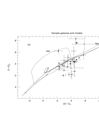
Figure 5: Color-color diagrams of the sample galaxies, with various models from BC93, differing by star formation histories: the decay time of each model is indicated. ssp means an instantaneous burst of star formation. ‘9’ indicates the point where the age of the model is 1 Gyr. All the models have a Salpeter mass function (with a mass range of 0.1–125M_⊙). Other IMFs do not differ significantly from this and are not depicted here.

It is clear that all the models, except for the instantaneous burst, lie roughly on the same track. Models with longer decay times have bluer colors for the same age of the stellar population. The galaxies may have different ages and star formation histories, and they are fitted, practically, by all the models, although the fit is rather poor. This confirms again that broad-band colors alone do not contain enough information to resolve the star formation properties of the galaxies. Information in the UV or H$\alpha$ is needed, since these bands are much more sensitive to the recent star formation, as the ionizing/short band radiation is emitted mostly by stars with short lifetimes.

BC93 provide the number of LyC photons at all stages of development. We can use this to derive a distance-independent parameter for the sample galaxies:

$$[H\alpha-V]=-2.5\log[F(H\alpha)]-v\ ,$$ (6)

where F(H$\alpha$) is in $erg/cm^{2}/s$ and $v$ is the apparent V magnitude. This gives the ratio of line to continuum radiation, which is essentially the same as $EW[H\alpha]$, except for the wavelength of the continuum radiation.

Assuming a simple case B hydrogen recombination theory (Osterbrock 1989), with $T_{e}\simeq$10000K, the H$\alpha$ luminosity is coupled to the flux of LyC photons by:

$$N_{c}=7.43\times 10^{11}L(H\alpha)$$ (7)

with L(H$\alpha$) in erg/s. Equation 7 does not account for the fraction of LyC photons extinguished by dust, or which escape through gaps in the surrounding gas, or through the gas itself, as this fraction is relatively small and does not affect our interpretation. Therefore:

$$(H\alpha-V)=129.8-2.5\;\log[N_{c}]-V$$ (8)

where $\log[N_{c}]$ and V are those provided by BC93. ’Color-color’ diagrams, with (H$\alpha$ –V) as one of the colors, are very useful for tracing the star formation processes, because the H$\alpha$ luminosity changes by orders of magnitudes during the lifetime of a galaxy. Such diagrams are displayed in Figs. 6, 7 and 8.

Figure 6: H$\alpha$ –V vs. B–V, with BC93 models. For each decay time two models are depicted. The solid lines are Salpeter IMF and the dashed lines represent Scalo’s (1986) IMF. The ssp model with Scalo IMF is not displayed, as it is very similar to the Salpeter model. The numbers indicate the log(age) in years only near the Salpeter models, for clarity. The symbols are the same as in previous color-color plots, and a fiducial error bar is at the lower right corner.

Figure 7: H$\alpha$ –V vs. V–R, with notations the same as before.

Figure 8: H$\alpha$ –V vs. R–I, with notations the same as before.

The figures show that the B–V colors are consistent with the models, while the V–R and R–I colors are bluer than expected. This can also be seen in Figs. 5a and 5b, where the points lie, on average, below the predicted curves. What could the reason for this deviation? A reasonable possibility is extinction by dust, that reddens the galactic colors. Extinction effects, however, will move the points more or less along the curves of Figs. 5, even when considering different dust geometries and extinction laws, i.e., the differences which arise due to various dust configurations are insignificant compared to the deviation seen here. The ‘color excess’ E(H$\alpha$–V), which was not taken into account in our derivation of (H$\alpha$–V), should typically be $\sim 0.3\;mag$, according to the considerations discussed above. This is less than the typical error displayed in Figs. 6, 7 and 8, and thus does not affect our interpretation. Therefore, dust extinction is not likely to be the reason for the mismatch between models and the observed parameters.

As for the LyC radiation that may escape from the HII regions due to a partial coverage by hydrogen clouds, or due to their insufficient optical depth, a realistic assumption would be that at most 50% of these photons can escape. This translates to 0.75 $mag$, which, together with the 0.3 $mag$ extinction, may reduce by 1.05 $mag$ the observed value of H$\alpha$–V. This, again, is not sufficient for bringing the observed results in accordance with the models.

Another effect may be the influence of a strong H$\alpha$ line on the R band result. This will make the V–R color redder than the line-free color, and move R–I to bluer values, an effect that may explain the R–I vs. V–R diagram. In the V–R vs. B–V diagram, however, this effect should move the points toward redder V–R color relative to their original locus, in the opposite direction to what is seen here. In any case, only the bluer galaxies should show this effect, which cannot change the colors by more than 0.1$\;mag$, not enough to explain the deviation seen in Fig. 8. In paper I we have mentioned that our B–V results are redder by $\sim 0.1\;mag$, on average, than other published data for some VCC galaxies. This is not explained by an observational bias, but even if such a bias exists, and allowing systematic errors of $0.1\;mag$ or even more in R–I, we cannot account for the difference between our results and the various models. Therefore, we conclude that the galactic broad-band colors and H$\alpha$ data of our sample galaxies cannot be explained, as a whole, by a single age stellar population model. This rejects, with a significant degree of confidence, our working assumption.

The spectra of the stellar populations calculated by BC93 are a superposition of spectra of individual stars, weighted according to the IMF. In young star-forming regions, however, the contribution of the nebulosity is significant, mostly producing the emission lines and also affecting the continuum. This is not included in models such as of BC93. Mas-Hesse & Kunth (1991, MHK) calculated observable parameters of starburst regions relying on stellar evolutionary tracks with Z=Z_⊙ and Z=Z_⊙/10 metallicities and using short time steps of $\geq$0.05 Myr. Their models include, along with the stellar contribution, the radiation of the surrounding gas and dust. They provide, among other parameters, H$\beta$ luminosities and rough SEDs of 0 – 20 Myr old burst populations with different IMFs and metallicities. The contribution of the nebulosity to the continuum is $\sim$30% in R and $\sim$10% in V during the first few $10^{6}$ years, and is more pronounced for low metallicity populations. It is, thus, important to consider this effect on the broad-band colors.

We calculated from the SEDs given by MHK the approximate broad-band colors B–V, V–R and R–I, where R and I are the Johnson bands, by scaling to the flux densities at each central wavelength of a normal zero magnitude star from Allen (1973). In addition we calculated (H$\alpha$ –V), using the case B line ratio $H\alpha/H_{\beta}=2.86$ to estimate the H$\alpha$ contribution.

As the nebulosity contribution rapidly decays after $10^{7}$ years, the BC93 models describe well the galactic properties after the SFR has dropped significantly. We should consider, therefore, a combination of the two models, since in most sample galaxies we have star-forming regions residing within an older stellar population, and the models of MHK account for only the first 20 Myr after the burst. Figs. 9, 10 and 11 are the same as Figs. 6, 7 and 8, with fewer BC93 models and two models from MHK. These models are for solar metallicity Z_⊙ and Z_⊙/10, with IMF slope $\alpha=2$ and upper mass cutoff of 120 M_⊙. Other models, with Z_⊙, are not significantly different from those displayed.

Figure 9: H$\alpha$ –V vs. B–V, with BC93 models and Mas-Hesse & Kunth (1991) models for solar and low metallicities.

Figure 10: H$\alpha$ –V vs. V–R, with notations the same as before.

Figure 11: H$\alpha$ –V vs. R–I, with notations the same as before.

While the solar metallicity models are not dramatically different from the ssp BC93 model, the Z_⊙/10 model is. The low metallicity model can explain our results, as it has bluer colors for galaxies with the same H$\alpha$ line strength. The low metallicity model, together with the BC93 models, bracket the observational points. We use a simplified two population scenario, considering the two populations on the diagrams in Figs. 9, 10 and 11, and identifying where their combination falls on the diagrams, with several relative weightings. Naturally, the result of the combination lies on a monotonous curve joining the two points, each representing one population, but the logarithmic scale may be misleading.

Figure 12: Same as previous figures, with two population curves (dashed lines) joining the low metallicity MHK model with the BC93 ssp model. These curves represent a mixture with varying ratio of two stellar populations, each located at one of the ends of the curves.

We calculated combinations of MHK and BC93 models for different V-band weightings of 1:12.5, 1:3, 1:1, 3:1 and 12.5:1 between the two populations in the color-color diagrams of Figs. 9 and 10. Joining the results of these calculations yields a rough curve along which the color indices of two populations fall in the color-color diagram. In figures 12a and 12b we added such ‘two population curves’, connecting the low metallicity MHK model with ages $\sim$3 and $\sim$13 Myr to the BC93 ssp model with ages 1 and 2 Gyr. These curves are represented by the thick, dashed lines in the figures. These lines bracket almost all the galaxies in our sample. The results indicate that the Virgo BCD galaxies may be described as a combination of a young, low metallicity stellar population of age 3–13 Myr with an older 1–2 Gyr population, that also originated in a burst of star formation (the metallicity factor is less significant for the older stellar population, therefore it is justified to combine the low metallicity young population with the old population which has solar metallicity).

In our derivation, the populations were weighed by their relative V-band luminosities. It is more adequate, however, to interpret the relative weight in terms of mass. However, due to the rapid evolution of the massive stars, which provide the bulk of the V-band luminosity at the early stages of a burst, we can only say that for a galaxy located mid-way between the two populations only 0.25–5% of the mass would be in the young burst. The derived mass ratio of the two populations depends also on the models used, a fact which, again, demonstrates the inaccuracy of such a derivation. Thus, the two population curves in Figs. 12 should be taken as indicative, and it is clear that for most galaxies most of the mass is in the older stellar population.

It should be noted, regarding this picture, that in practice, the older population was not created by a zero duration burst, but rather by a finite length burst. We may use our data to constrain the length of the burst that produced the older stars. From Figs. 12a and 12b it appears that a slowly decaying SFR population like the 4Gyr one cannot account for the sample galaxies. A two-population curve drawn from it to the low metallicity model, or to any other model, will not bracket all the galaxies in both diagrams. We may, thus, conclude that the older stars in the sample galaxies are likely to have originated in an exponentially decaying star formation process of at most $\sim$0.2 Gyr decay time. Similar behaviour is seen in the (H$\alpha$–V) vs. (V–I) diagrams.

One can also note that the locus of the data points seems to be different regarding the weighting of the young and old populations from one color to the other. In (B–V) they are more condensed in the center, while in (V–R) and (R–I) they are more dispersed and seem to be closer to the young, low metallicity models. We estimate that this might be due to uncertainty and incompleteness of the models and/or some biases of our broad-band results. As discussed in paper I and above, we believe the robustness of our results, and in any case a bias of $\sim 0.1\;mag$ will not alter our conclusions concerning the two population scenario.

This scenario, although simple, indicates general star formation characteristics of the sample galaxies. Obviously, the galaxies are not identical, neither in their metallicity, nor in their SFR and their dust extinction. The latter increases the scatter of the observed data points. However, the conclusion is that some of the galaxies, particularly the bluer ones, must have metallicities considerably lower than the solar value. This finding is not new and is in agreement with data for other BCD galaxies (e.g., Kunth & Sargent 1986).

The star formation process in these galaxies, with no connection to whether they are BCDs or earlier types, is likely to occur in short duration episodes and the previous episodes probably appeared in the last 1–2 Gyr. Actually, it is more probable that a few episodes, or bursts have occurred during the lifetime of the galaxies, rather than just a single one. This is consistent with other results for blue galaxies, e.g., Huchra et al. (1983), Fanelli et al. (1988) and Deharveng et al. (1994), which trace a burst population with an underlying older population. We can, with a reasonable degree of confidence, rule out the possibilities that slowly decaying past star formation activity is present in these dwarf galaxies.

It is worth mentioning that the two-population approach with BC93 models alone cannot explain the data points in all diagrams simultaneously. It is possible, in principle, to explain the points in a certain color-color diagram by a combination of two populations, but combinations of different populations are needed in other diagrams. This indicates that no solar metallicity model can explain the results of our sample as a whole.

The low metallicity picture can have an alternative explanation, however, if the LyC photons in the HII regions are heavily extinguished by dust, or just escape the regions. This is in contrast to the general picture accepted today, but, as pointed out by MHK, we do not know exactly by how much is LyC extinguished. If the original ionizing photons are extinguished by an order of magnitude, this will bring the observed data points in accordance with the (two population combination of) solar metallicity models.

This explanation can be tested using the available IRAS data for some of the sample galaxies. The five H$\alpha$-brightest galaxies of our sample have IRAS fluxes in both the 60$\;\mu$m and 100$\;\mu$m bands. We can estimate the SFR in these galaxies from the FIR data, using the method of Thronson & Telesco (1986). This method is based on the assumption that essentially all of the luminosity of the massive OB stars is absorbed by the dust and is reemitted in the infrared. This yields the following relation:

$$SFR=6.5\times 10^{-10}L_{IR}\ ,$$ (9)

where the FIR luminosity, $L_{IR}$, which is given in solar units, can be approximated by:

$$L_{IR}\approx 6\times 10^{5}D^{2}(2.58f_{60}+f_{100})$$ (10)

where $D$ is the distance to the object in Mpc, and $f_{60}$ and $f_{100}$ are the two IRAS flux densities, in Jy. The resulting SFR is lower by a factor of two than that derived from H$\alpha$. This discrepancy can be caused by three possible reasons:

1. Our adopted value of a factor of two, for the H$\alpha$ flux extinction may be an overestimate.

2. There are discrepancies in the models, such as IMF slope, high mass cutoff, and estimates of parameters such as the lifetimes of massive stars and their LyC and total luminosities.

3. Not all the luminosity of the massive stars is absorbed by the dust, in particular the LyC radiation is not absorbed by it, as the ambient gas is a more efficient absorber in these wavelengths, or, the dust does not reside inside the line-emitting region at all.

It is evident that the first reason alone cannot account for this mismatch. This is because only the extreme case of no dust at all would bring the H$\alpha$-estimated SFR in agreement with the FIR-estimated value. No dust means practically no FIR radiation, thus there should be no FIR radiation from the objects. Adopting a more moderate approach of low optical depth of the dust, will bring the results closer to each other, but never bring them to a complete agreement. It is, thus, possible that we have overestimated the dust extinction of the H$\alpha$ line radiation, though not by a very large extent. We prefer to retain our adopted value of dust extinction for further discussion.

Therefore the other two reasons mentioned above must play some role in changing the estimated SFR value. Although it is not possible to disentangle the influence of these two effects, they are both inconsistent with the LyC radiation being heavily absorbed by the dust. If LyC photons are extinguished by dust, this would result in a significantly higher FIR radiation while the H$\alpha$ flux would be further reduced, opposite to the situation observed here. This finding strengthens the scenario that the LyC radiation is not extinguished significantly in the cores of HII regions.

The comparison between the FIR and H$\alpha$ radiation sheds light upon the optical depth of the hydrogen clouds and their covering factor. If the HII regions are not ionization bound, this will cause a reduction of the H$\alpha$ flux and may enhance the FIR emission from the galaxies, because the LyC photons that escape the HII regions are likely to be absorbed by more distant diffuse dust. This dust will re-radiate its energy in the FIR. Again, the effect is opposite to the current situation, a fact which strengthens our assumption that nearly all the LyC flux is absorbed by the hydrogen.

It is clear that different IMFs influence the observational parameters less than the metallicity and age of a stellar population, but with the dispersion of our data points, and with many additional parameters, it is practically impossible to determine the IMF of the galaxies. Other factors, like gas recycling in the model galaxy, are even less significant and cannot be tested here.

In addition to the H$\alpha$ data, it is important to consider the UV data available for some of our galaxies. The UV radiation (at $\lambda\geq$ 1300Å, in our case) is also emitted mostly by the young massive stars and is more sensitive to the star formation properties of the galaxies than the optical colors. We calculated, for the galaxies which have UV data, the (UV–V) color (UV is the monochromatic magnitude at $\sim$1650Å, as discussed in paper I). We corrected these values for dust extinction, according to the value in section 2, and compare them to the ”14–V” color, given by BC93 for the HST-UV14 filter. In Fig. 13 the galaxies are plotted in the (UV–V) vs. (R–I) plane, together with BC93 models. The galaxy VCC1374, which has a faint UV upper limit, is bright in H$\alpha$ and in the optical.

The UV results are consistent with our previous interpretations for the star formation properties of the galaxies. The same trend is observed as in the H$\alpha$ data for the three colors B–V, V–R and R–I, and only the latter is displayed here with the UV data. Unfortunately, only few galaxies have significant UV fluxes from IUE or from FAUST observations.

Figure 13: UV–V vs. R–I for the sample galaxies, together with models from BC93. Galaxies with significant UV results are marked by filled squares, and those with UV upper limits as open circles. For clarity, not all upper limit arrows are drawn. For the theoretical UV we use the data of HST-UV14 filter given by BC93.

Instead of a color-color diagram, it may be useful to consider the entire SEDs of the galaxies, as derived in paper I. Since our derived SEDs are very sparse because of the broad-band colors, they cannot be tested against detailed spectra, but maybe compared, in general, with typical SEDs of different stellar populations. Using the set of spectra published by BC93, it can be noted that the galaxies VCC144, VCC1725 and VCC1791, which are the UV and H$\alpha$-brightest in our sample, may correspond to a young stellar population $\sim$0.1–0.3 Gyr old, regardless of the details of the star formation history. The situation of VCC10, VCC22 and VCC24 is less clear, however, since their SEDs are relatively flat in the optical, and may correspond to an age of 4–13 Gyr.

The question that arises at this stage concerns the difference among the various sample galaxies in terms of their star formation. In light of the interpretation of the results discussed above, of a very young, low metallicity, stellar population residing within (probably a larger region which contains) an older stellar population, we conclude that the difference lies in the relative weight of the two populations (in terms of their V magnitude, in our method of derivation). In the bluer and H$\alpha$-brighter galaxies, the young stars currently forming dominate the entire spectrum of the galaxy (although not necessarily dominating the mass), while in the red, H$\alpha$-faint objects, the star formation is relatively weak and the galactic colors are determined more by the older stellar population. As discussed above, the older stellar population is believed to have originated in one or more $\sim$instantaneous bursts of star formation.

The arguments presented above lead to the conclusion that all the sample galaxies, classified as BCDs or Im III–IV, or even earlier types, are basically of the same type, in which the star formation appears in bursts, but which are observed at different epochs of their lifetimes - some during the burst and others at a relatively quiescent epoch. In this context, galaxies like VCC1725, VCC1791 and VCC144 are examples of strong star-forming galaxies, in which the underlying older stellar population does not contribute much to the SED. In VCC144 there is hardly a sign of the older stellar population, and we conclude that this galaxy may be experiencing its first star formation burst (Brosch et al. 1997). On the other hand, VCC10, VCC22 and VCC24 are examples of galaxies in which the older stellar population dominates the SED.

Although this conclusion is not new, it is nicely supported by our results. If we could identify all the galaxies of this same type, maybe all the low-metallicity dwarfs, we would be able to conclude how often a burst takes place in these galaxies. To be more precise, we would be able to determine the duration of the burst period relative to the quiescent period from the fraction of high SFR galaxies observed in the entire sample.

3.3 Life expectancy of the galaxies

A starburst galaxy is one in which the current SFR is very high, relative to its average past SFR. Another indicator of a starburst galaxy is its gas consumption time. This is the time by which all the hydrogen available for star formation will be exhausted, assuming the current SFR is maintained. If this consumption time is considerably shorter than one Hubble time, the galaxy is probably experiencing a starburst. The current high SFR must then be a transient situation, after which the galaxy is expected to return to a ‘normal life’, as far as the SFR is concerned.

The gas consumption time, or ”Roberts time” (Sandage 1986), is given by: $\tau_{R}=\frac{M_{gas}}{SFR}$, where $M_{gas}$ is the total mass of interstellar gas in the galaxy. For the derivation of Roberts times of the sample galaxies, we used their HI mass from paper I. The total hydrogen mass may be at most $\sim$20% higher than the HI mass, as in late-type galaxies the H₂ is only a small part of the total hydrogen content (Young & Knezek 1989).

Table 2: HI properties of VCC galaxies.

In Table 2 we tabulate the HI properties of the sample galaxies. The distribution of Roberts times is presented in Fig. 14, where the galaxies classified as ”BCD” or ”BCD?” in VCC are marked in black. Clearly, many of the galaxies are starbursts, 10 out of 14 having a gas consumption time smaller than 1 Gyr. Even when including the maximally possible H₂ mass contribution, the times are rather short.

Figure 14: Histogram of the gas consumption times for VCC galaxies. The entire sample is shown, and BCDs are in black. The extension of the gas consumption time, due to the contribution of H₂ at 20% of the HI, is indicated by an arrow. This represents an upper limit to the H₂ contribution (see text).

The Roberts’ times are not the real life expectancies of the galaxies, even with the present SFR, because gas recycling may extend considerably the star formation. The factor by which the recycling prolongs the life expectancy of the galaxies depends basically on three parameters:

1. The fraction of mass returned to the interstellar medium by a single age stellar population,

2. The efficiency of converting the available gas to stars, and the dependence of the SFR on the gas density,

3. The amount of hydrogen available originally.

The gas return fraction strongly depends on details of the IMF, metallicity etc. Thus, it is difficult to assess the exact effect of recycling on the star formation of these galaxies. For disk galaxies, Kennicutt et al. (1994) obtained a range of 1.5–4 for this prolonging factor. If we adopt these values here we obtain a typical expected lifetime shorter than 2–4 Gyr, which is relatively short. In irregular galaxies, in contrast to large disk galaxies, a large fraction of the HI extends beyound the optical size, where the star formation activity is taking place. This will reduce the future lifetime of the galaxies even further, provided that no star formation will start outside the visible optical radius. Thus, the uncertainty of the expected future lifetimes of the galaxies in our sample is rather large, but still there is a strong indication of a starburst ongoing in these galaxies.

This result supports our picture of objects in which the star formation appears in bursts. The real future lifetime of the galaxies depends on the duration of the starbursts and the time interval between bursts. This question is still open, although our interpretation indicates that previous bursts probably happened in most of the galaxies during the last Gyr.

3.4 Star formation mechanisms

The question that is raised by the above discussions is how do the different star formation inducing mechanisms govern the star formation in the late-type dwarfs of our sample. Any answer to this question can only be found by a large survey, which encompasses all galactic types. However, as derived here, once the star formation activity is triggered, its intensity, as manifested by the SFR/area, appears similar in small and large galaxies. This indicates that small-scale mechanisms, believed to dominate in dwarf galaxies, are as efficient as the large-scale mechanisms acting in large galaxies.

A note should be made, however, concerning the comparison of the SFR/area in our galaxies with that in large disk galaxies, where the intensive star formation process is confined to a few hundred pc. thick disk. This is because dwarf galaxies are generally amorphous and diskless, thus their observed SFR/area is actually the ‘column density’ of the SFR. It would be more appropriate to characterize the intensity of the star formation process in these galaxies by spatial density rather than by surface density, which, of course, is not possible here. One should note, however, that the actual thickness of a dwarf galaxy may not be too different from that of a disk in a large galaxy, thus the comparison may not be totally out of order.

Another phenomenon, believed to trigger star formation in clusters of galaxies, is the gravitational tide from a neighboring galaxy, which is strongest near the cluster core where galactic encounters are more frequent. Tidal forces can trigger star formation also in field galaxies with close companions - many field starburst galaxies are found to be interacting with companions. It is, thus, natural to expect a relation between the star formation properties of the sample galaxies and their distance from the center of the Virgo cluster. The star formation is expected to be more pronounced in galaxies that are close to the center. However, no significant correlation was found between the Virgocentric distance and any of the star formation parameters. If anything, the SFR seems to increase with increasing Virgocentric distance, while the SFR/area does not show any correlation. The SFR/area also does not show any correlation with the recession velocity of the galaxies. This implies that tidal forces near the core of the Virgo cluster are not significant relative to other mechanisms triggering star formation in dwarf galaxies.

An additional cluster effect, which may influence the star formation properties, is the stripping of interstellar matter from galaxies that pass near the cluster core (e.g., Haynes et al. 1990). Galaxies near a cluster core are found to have less HI than galaxies further away from the core. The high HI galaxies of our sample, which are more than 6^∘ away from the center, have higher HI flux, on average, than those closer than 6^∘. This can be seen also in Fig. 2 of paper 1, where the low HI galaxies are distributed more or less evenly, while the high HI galaxies appear only in the outer parts of the cluster. This effect is also seen using a larger sample of Virgo dwarfs from Hoffman et al. (1987, 1989).

The gas-stripping phenomenon may affect the star formation in the galaxies studied here in an opposite direction to that of tidal forces discussed above, the amount of HI available to form stars being less near the core than away from it. We believe it would be an overinterpretation of the data, however, to say that the apparent increase in SFR with Virgocentric distance is due to this effect.

4 Conclusion

The main goal of this study is to investigate mechanisms that govern star formation processes in galaxies and their dependence on various galactic parameters. The intention in focusing on our sample of late-type dwarfs in the Virgo cluster was to exclude some of these mechanisms thought to be responsible for star formation in large galaxies. In addition, we concentrate on cluster members to test for effects of the cluster environment on the star formation properties of the galaxies.

The observational data used to evaluate the star formation parameters, such as the SFR, IMF, and star formation history, are affected primarily by the internal dust extinction in the galaxies. This depends on the amount and distribution of dust in the galaxy. We adopted general correction parameters for the entire sample to account for the effects of dust.

Using a data base consisting of a number of broad band colors and H$\alpha$ observations it is possible to track the ongoing star formation process, as well as the star formation history of the sample. This is done for both low HI and high HI subsamples, which enables one to check the dependence of these parameters on the neutral hydrogen content of the galaxies. In all cases, no significant dependence of the star formation properties on the HI content was found. This may be explained by the following argument: the differences among the various galaxies in our sample lie in the relative weight of the flux originating from their ‘current’ and ‘previous’ star formation episodes. Since the hydrogen is depleted during each such burst of star formation, its current amount depends on the number of bursts that occurred in the past, as well as on the original amount present. The strength of the current starburst apparently does not depend on this star formation history and, thus, cannot be correlated with the neutral hydrogen content.

Considering the entire set of observations, together with various population synthesis models, a star formation scenario can be sketched for the sample galaxies. The process of star formation in late-type dwarf galaxies takes place in short bursts, presumably much shorter than 1Gyr (10–100 Myr). The past burst(s) probably occurred within the last $\sim$Gyr. Redder galaxies can be fitted with a single, longer burst with this decay time (1 Gyr), but the observational data of the entire sample can only be explained in terms of a series of short bursts. In this picture, the difference among galaxies lies in the relative weight of the starburst and the older population. This depends on the age and size of the current burst and of former bursts, therefore the dwarf galaxies may be seen as a single type, which are observed at different epochs of their evolution.

In addition, the galaxies appear to have low metal abundance, mainly from their blue R–I color. This is in agreement with previous data for irregular dwarf galaxies, known to have typically low metallicities (e.g., Kunth & Sargent 1986). A low metallicity of a galaxy indicates its young age, since the amount of heavy elements produced by massive stars increases during the lifetime of the galaxy, which implies that some of our sample galaxies are genuinely young. This also is not a new finding (see Gondhalekar et al. 1984). A development trend can be sketched, in which the galaxies undergo a series of starbursts, and their metallicity increases from one burst to the other. Since the HII regions in many of the galaxies occupy a large fraction of the galactic volume, it is possible that each burst changes significantly the total galactic metal abundance. The relation between the fraction of the galactic surface covered by H II regions and star formation properties will be discussed in a subsequent paper.

We have tested the cluster influence on the sample galaxies’ star formation properties. No correlation was found between the Virgocentric distande of the galaxies and any of their star formation properties. This may manifest the low significance of tidal forces when acting on dwarf galaxies. It can be understood as these galaxies are small in size and, thus, a gradient in an external gravitational field induced by another galaxy may not cause a great difference from side to side relative to the galaxy’s own gravitational well. This finding is, therefore, not surprising.

A remarkable galaxy in our sample is VCC144. It has strong SFR and an exceptional SFR/area, compared with the other galaxies. It is also the only object in which the burst population is believed to dominate in luminosity and in mass over older populations, if any. However, it does not show any special behavior in other parameters such as the HI flux, velocity dispersion, infrared flux, or distance from cluster center, in which it seems a ‘normal’ object in the sample. It is the most condensed object of our sample, in terms of star formation, but with no other peculiarities. It is possible that this object is experiencing its very first burst of star formation, which indicates that galaxies are still being formed these days in the Virgo cluster.

To conclude - the star formation in late-type dwarf galaxies in the Virgo cluster occurs probably in bursts. The bursts do not seem to depend on galactic history or on cluster environment. The details of the IMF of the burst population cannot be determined from the data collected in this study, but a general scenario of the galactic evolution is sketched. During their lifetime, the galaxies evolve from late-type to earlier type, their metallicity increases, and they become redder objects in the optical.

References

Allen, C.W. 1973, Astrophysical Quantities, The Athlone Press, University of London.

Brosch, N., Almoznino, E. & Hoffman, G.L. 1997, Astron. Astrophys. in press.

Bruzual, G.A., & Charlot, S. 1993, Astrophys. J. 405, 538 (BC93).

Buat, V., Deharveng, J.M. & Donas, J. 1989, Astron. Astrophys. 223, 42.

Calzetti, D., Kinney, A.L. & Storchi-Bergmann, T. 1994, Astrophys. J. 429, 582.

Deharveng, J. M., Albrecht, R., Barbieri, C., Blades, J. C., Boksenberg, A., Crane, P., Disney, M. J., Jakobsen, P., Kamperman, T. M., King, I. R., Macchetto, F., Mackay, C. D., Paresce, F., Weigelt, G., Baxter, D., Greenfield, P., Jedrzejewski, R., Nota, A., Sparks, W. B. 1994, Astron. Astrophys. 288, 413.

Fanelli, M. N., O’Connell, R. W., Thuan, T. X. 1988, Astrophys. J. 334, 665.

Fernie, J.D. 1983, PASP 95, 782.

Gallagher, J.S., Hunter, D.A. & Tutukov, A.V. 1984, Astrophys. J. 284, 544 (GHT).

Gondhalekar, P.M., Morgan, D.H., Dopita, M. & Phillips, A.P. 1984, Mon. Not. R. astr. Soc. 209, 59.

Haynes, M.P., Herter, T., Barton, A.S. & Benensohn, J.S. 1990, Astron.J. 99, 1740.

Hoffman, G.L., Helou, G., Salpeter, E.E., Glosson, J. & Sandage, A. 1987, Astrophys. J. Suppl. 63, 247.

Hoffman, G.L., Williams, H.L., Salpeter, E.E., Sandage, A. & Binggeli, B. 1989, Astrophys. J. Suppl. 71, 701.

Huchra, J. P., Geller, M. J., Gallagher, J., Hunter, D., Hartmann, L., Fabbiano, G., Aaronson, M. 1983, Astrophys. J. 274, 125.

Kennicutt, R.C. 1983, Astrophys. J. 272, 54 (K83).

Kennicutt, R.C. & Kent, S.M. 1983, Astrophys. J. 88, 1094.

Kennicutt, R.C. 1989, Large Scale Star Formation & the Interstellar Medium, in ”The Interstellar Medium in External Galaxies”. ed. H.A.Thronson & J.M.Shull.

Kennicutt, R.C., Tamblyn, P. & Congdon, C.W. 1994, Astrophys. J. 435, 22.

Kunth, D. & Sargent, W.L.W. 1986, Astrophys. J. 300, 496.

Larson, R.B. 1987, Star Formation Rates & Starbursts, in ”Starbursts & Galaxy Evolution”. ed. T.X.Thuan, T.Montmerle & J.T.T.Van (Edition Frontieres, Gif sur Yvette - FRANCE).

Mas-Hesse, J.M. & Kunth, D. 1991, Astron. Astrophys. Suppl. 88, 399.

Miller, G.E. & Scalo, J.M. 1979, Astrophys. J. Suppl. 41, 513 (MS79).

Osterbrock, D.E. 1989, Astrophysics of Gaseous Nebulae & Active Galactic Nuclei, (Mill Valley, CA: University Science Books).

Pogge, R.W. & Eskridge, P.B. 1987, Astrophys. J. 93, 291 (PE87).

Salpeter, E.E. 1955, Astrophys. J. 121, 161 (S55).

Sandage, A. 1986, Astron. Astrophys. 161, 89.

Savage, B.D. & Mathis, J.S. 1979, Ann. Rev. Astron. Astrophys. (SM).

Scalo, J.M. 1986, Fundamentals of Cosmic Physics 11, 1 (S86).

Schmidt, M. 1959, Astrophys. J. 129, 243.

Shields, G.A. 1990, Ann. Rev. Astron. Astrophys. 28, 525.

Terlevich, R. & Melnick, J. 1983, ESO preprint no. 264.

Thronson, H.A. & Telesco, C.M. 1986, Astrophys. J. 311, 98.

Young, J.S. & Knezek, P.M. 1989, Astrophys. J. Lett. 347, L55.