MICROLENSING

Abstract

Microlensing observations have now become a useful tool in searching for non–luminous astrophysical compact objects (brown dwarfs, faint stars, neutron stars, black holes and even planets). Originally conceived for establishing whether the halo of the Galaxy is composed of this type of objects, the ongoing searches are actually also sensitive to the dark constituents of other Galactic components (thin and thick disks, outer spheroid, bulge). We discuss here the present searches for microlensing of stars in the Magellanic Clouds and in the Galactic bulge (EROS, MACHO, OGLE and DUO collaborations). We analyse the information which can be obtained regarding the spatial distribution and motion of the lensing objects as well as about their mass function and their overall contribution to the mass of the Galaxy. We also discuss the additional signals, such as the parallax due to the motion of the Earth, the effects due to the finite source size and the lensing events involving binary objects, which can further constrain the lens properties. We describe the future prospects for these searches and the further proposed observations which could help to elucidate these issues, such as microlensing of stars in the Andromeda galaxy, satellite parallax measurements and infrared observations.

To appear in Physics Reports

SISSA–171/95/EP

1 Introduction

The bending of light in a gravitational field predicted by general relativity provided one of the first verifications of Einstein theory [1]. The value of the deflection angle which results has now been tested at the 1% level by observing the change in the apparent position of stars whose light is deflected by the Sun. In 1920, Eddington [2] noted that the light deflection by a stellar object would lead to a secondary dimmer image of a source star on the opposite side of the deflector. Chwolson [3] later pointed out that these secondary images could make foreground stars appear as binaries, and that if the alignment were perfect, the image of the source would be a ring. In 1936, Einstein [4] published the correct formula for the magnification of the two images of a very distant star, and concluded that this lensing effect was of no practical relevance due to the unresolvably small angular separation of the images and the low probability for a high amplification event to take place.

The following year, Zwicky [5] showed that, if the deflecting object were a galaxy instead of a single star, the gravitational lensing of the light of a background galaxy would lead to resolvable images. This ‘macrolensing’ effect would provide information about the mass of the intervening galaxy and allow observation of objects at much larger distances due to the magnification of their light. Furthermore, the probability that this effect be observed is a ‘certainty’ [6].

It was actually the multiple imaging of a high redshift quasar by a foreground galaxy which provided the first observation of gravitational lensing [7], and this area of research has now become an active field in astronomy, with the potential of giving crucial information for cosmology [8, 9, 10]. For instance, the time delay among the multiple images of a quasar allows one to relate the lens mass to the Hubble constant. Another interesting example is that the mass distribution of a rich cluster can be reconstructed from the shapes of the images of thousands of background faint blue galaxies around it, which become elongated due to the effect of weak lensing by the cluster [11]. Also, gravitational lensing can strongly affect the observable properties of AGN and quasars, and may have to be taken into account when inferring their intrinsic properties.

While these developments were going on, the theoretical study of gravitational lensing of stars by stars restarted in 1964, with the work of Liebes [12] and Refsdal [13], who extended the formalism and discussed the lensing of stars in the disk of the Galaxy, in globular clusters and in the Andromeda galaxy.

The lensing effect of individual stars belonging to a galaxy that is itself macrolensing a background source was discussed by Chang and Refsdal [14]. When both the lensed source and the intervening galaxy are at cosmological distances, the passage of one of these stars close to the line of sight to one of the images further deflects the source light by an angle which is typically of ${\cal O}(\mu$arcsec). The name ‘microlensing’ (ML) then became associated with this process, and is now generally applied to any gravitational lensing effect by a compact object producing unresolvable images of a source and potentially huge magnifications of its light.

Press and Gunn [15] showed in 1973 that a cosmological density of massive compact dark objects could manifest through the ML of high redshift sources. In 1981, Gott [16] pointed out the possibility of detecting the dark halos of remote galaxies by looking for ML of background quasars. It was in 1986 that Paczyński [17] gave a new face to the field when he noted that, by monitoring the light–curves of millions of stars in the Large Magellanic Cloud (LMC) for more than a year, it would become possible to test whether the halo of our galaxy consisted of compact objects with masses between $10^{-6}$ and $10^{2}\ M_{\odot}$, i.e. covering most of the range where baryonic dark matter in the form of planets, Jupiters, brown dwarfs or stellar remnants (dead stars, neutron stars or black holes) could lie. It was later realized [18, 19] that the Galactic bulge stars also provided an interesting target to look at, since at least the lensing by faint stars in the disk should grant the observation of ML events, and observations in the bulge could also allow one to test the dark constituency of the Galaxy close to the Galactic plane.

With these motivations, several groups undertook the observations towards the LMC (EROS and MACHO collaborations) and towards the bulge (MACHO and OGLE), obtaining the first harvest of ML events in 1993 [20, 21, 22]. As will be discussed in this review, the observations at present are already providing crucial insights into the dark matter problem, into the non–luminous contribution to the mass of the different Galactic components and they are helping to unravel the morphology of the inner part of the Galaxy. The continuation of these programs, as well as the new ones entering the scene (DUO collaboration looking towards the bulge; AGAPE and the Columbia–VATT collaborations looking at Andromeda and followup telescope networks such as PLANET, GMAN and MOA looking for fine details in the microlensing events) will certainly allow us to reach a much deeper knowledge of these fundamental issues in the near future.

2 Galactic components and dark matter

In order to study the lensing effects of objects in and around the Galaxy, it is first convenient to discuss the nature of the several possible lens candidates as well as their distribution and expected properties. In this Section we briefly introduce the different Galactic components [23, 24, 25] and the possible lensing populations present in them.

2.1 Dark halos

The existence of dark galactic halos is directly related to the dark matter (DM) issue [26], namely the fact that more than 90%, and probably even 99%, of the matter in the Universe does not seem to emit any electromagnetic radiation. Its existence has been inferred from the gravitational effects that it has on the observed motions of gas, stars, galaxies and clusters, and also from its effects on the overall geometry of space–time.

For instance, the velocity dispersions of galaxies in clusters indicate that cluster masses are more than 10 times larger than the mass contained in the luminous parts of its constituent galaxies and in the intra–cluster gas [27, 28]. Similar conclusions are obtained from the X–ray observations of the cluster gas temperature profiles [28] as well as from weak gravitational lensing [11]. At Galactic scales, the presence of DM is most clearly indicated by the flatness of the rotation curves of spiral galaxies [29, 30], and also from the motion of satellite galaxies [31].

The existence of dark halos surrounding the visible galaxies is supposed to account, at least in part, for this missing mass (see e.g. Ref. [32]). The halo densities are then required to fall as $r^{-2}$ with the galactocentric distance $r$, as long as the rotation curves stay flat. A parameterization usually adopted for the density of a spherically symmetric halo is

$$\rho^{H}(r)=\rho^{H}_{0}{(R_{0}^{2}+a^{2})\over(r^{2}+a^{2})},$$ (1)

where $a$ is the halo core radius, typically a few kpc. For our galaxy, taking $R_{0}$ as the solar galactocentric distance, we have that in Eq. (1) $\rho_{0}^{H}$ is the local halo density. In the following we will adopt $R_{0}=8.5$ kpc and we will take the reference value $\rho_{0}^{H}\simeq 10^{-2}M_{\odot}/$pc³ [33, 25, 34].

If we assume that the Milky Way circular speed $v_{c}\simeq 220$ km/s stays constant up to a galactocentric distance $r_{max}$, the total mass of the Galaxy within that radius results ($G$ is Newton’s constant)

$$M_{tot}\simeq{v_{c}^{2}r_{max}\over G}\simeq 5.6\times 10^{11}\left({v_{c}\over 220\ {\rm km/s}}\right)^{2}\left({r_{max}\over 50\ {\rm kpc}}\right)M_{\odot},$$ (2)

which is an order of magnitude larger than the disk mass if $r_{max}>50$ kpc, and hence should mainly be due to the halo. The large amounts of matter contained in the dark Galactic halos may account for the missing mass in clusters as well.

The detailed profile and extent of galactic halos, in particular that of the Milky Way, are however not well known, partly due to the poor knowledge of the rotation curves. For our galaxy, the rotation curve has been measured only up to $\sim 20$ kpc and with large uncertainties [23]. There is also an uncertainty affecting the halo density in the inner region of the Galaxy which is related to the imprecise knowledge of the contribution to the rotation curve coming from the Galactic disk. For instance, maximum disk models [35] would lead to little halo mass inside the solar galactocentric radius.

Another poorly constrained property of halos is their ellipticity [36] which, for instance, in simulations of galaxy formation with cold dark matter turns out to be non–negligible. Observations of polar ring galaxies, in which the motion of gas in a ring orthogonal to the plane of the disk can constrain the flattening of the mass distribution, have also provided some examples of flattened halos. However, the flaring of HI in the outskirts of the disks in spiral galaxies indicates that the halo is not distributed as a thin disk [37, 38]. A further complication is that a flattened halo may not be axisymmetric and may also be tilted with respect to the disk plane.

Associated with all these uncertainties there is also an uncertainty in the motion of the halo constituents. The simplest hypothesis that is usually adopted is that the halo objects move with isotropic velocities, which have a Maxwellian distribution with constant (space independent) one–dimensional velocity dispersion $\sigma$, which is then related to the circular speed by $\sigma=v_{c}/\sqrt{2}\simeq 155$ km/s. This so–called isothermal sphere is known to lead to a density profile falling as $r^{-2}$ at large radii. A self–consistent halo distribution, not including the effects of the disk but allowing for an elliptical halo as well as for a rising or declining rotation curve, has been obtained in Ref. [39]. Some progress towards including the dynamical effects of disks and bulges has also recently been made [40].

2.2 Baryonic or non-baryonic?

The nature of the dark halo constituents is one of the important open problems of present–day physics. One possibility is that they are composed of just ordinary baryonic matter, e.g. protons and neutrons. A very important bound for the total amount of baryons in the Universe comes from the agreement between the observed abundances of light elements (D, ³He, ⁴He, ⁷Li) and those predicted in the context of the primordial nucleosynthesis theory. This requires that the average density of baryons $\rho_{b}$, in terms of the critical density of the Universe $\rho_{c}$, $\Omega_{b}\equiv\rho_{b}/\rho_{c}$, be in the range $0.009<\Omega_{b}<0.14$ [41]. Since luminous matter accounts for $0.003<\Omega_{lum}\leq 0.007$ [42, 43], the lower bound on $\Omega_{b}$ suggests the existence of baryonic matter in dark forms. The upper bound on $\Omega_{b}$ is consistent with dark baryonic halos accounting for the observations at galactic scales, which require $\Omega\geq 0.1$. However, when combined with observations on cluster scales or larger [44], which imply that $\Omega_{tot}>0.2$–0.3 (and probably $\Omega_{tot}\simeq 1$, which is the value preferred by inflationary theories), the above mentioned upper bound, $\Omega_{b}<0.14$, suggests the existence of non–baryonic dark matter (NBDM).

An additional attractive feature of NBDM is that it proves very useful in allowing for the formation of structure, in scenarios where the inhomogeneities in the density grow first in the NBDM, with the baryons falling later into the dark potential wells. In these scenarios, the NBDM that seeded galaxy formation is expected to remain somewhere in the galaxies, with the halo being the most ‘natural’ place. Candidates for NBDM abound in the literature, going from primordial black holes (made essentially out of radiation) to elementary particles such as massive neutrinos, axions, supersymmetric neutralinos, etc..

On the other hand, as mentioned above, halos may well be baryonic and there are actually many ways in which baryons can hide in dark forms, without entering into conflict with other observations (for a review see Ref. [45]). These are:

• Very massive black holes (with mass $m>200\ M_{\odot}$, in order to avoid the ejection of too many heavy elements into the interstellar medium).

• Stellar remnants, such as neutron stars or dead white dwarfs ($m\sim M_{\odot}$).

• Brown dwarfs, which are stars made essentially of H and He that are too light to start efficient nuclear fusion reactions ($m<m_{HB}\simeq 0.08\ M_{\odot}$, where $m_{HB}$ is the minimum star mass for H burning to take place). The Jeans mass, i.e. the minimum mass for which the gravitational forces of an isolated gas cloud fragment can overcome the pressure forces and lead to star formation, has been estimated to be 4–$7\times 10^{-3}\ M_{\odot}$ [46, 47]. Under special conditions (e.g. in protoplanetary disks), this lower bound can be evaded. Hydrogenous objects with masses in the neighbourhood of $10^{-3}\ M_{\odot}$ are usually named Jupiters.

• Snowballs, which are compact objects with masses below $10^{-3}\ M_{\odot}$, held together by molecular, rather than gravitational, forces. A lower bound of $10^{-7}\ M_{\odot}$ for their masses has been suggested in order to avoid their evaporation [48].

• Clouds of molecular H have been proposed as baryonic constituents of the dark Galactic halos [49, 50, 51].

These possibilities, with the exception of the last one, clearly provide excellent candidates for gravitational lenses. These objects are sometimes generically called Massive Compact Halo Objects (MACHOs). Of course nothing is known about the mass function of the halo constituents, except that the number of ordinary main sequence stars (see Section 6.3) and of white dwarf remnants [52] should be quite suppressed.

2.3 Galactic disk

Most of the visible stars in our galaxy are distributed in a disk, generally assumed to be a double exponential in the galactocentric cylindrical coordinates ($R,{\rm z}$)

$$\rho^{D}(R,{\rm z})=\rho^{D}_{0}\;{\rm exp}\left(-{R-R_{0}\over h_{R}}-{|{\rm z}|\over h_{\rm z}}\right),$$ (3)

where $\rho_{0}^{D}$ is the local disk density, $h_{R}\simeq 3.5$ kpc is the disk scale length [25] (estimates of $h_{R}$ vary however in the wide range from 1.8 to 6 kpc [53]) and $h_{\rm z}$ is the scale height, which is $\sim$100 pc for the very young stars and gas, and $\sim$325 pc for the older disk stars [54]. There are some indications [55] that at distances larger than $\sim 3$ kpc towards the Galactic center the disk star density falls below what would follow from Eq. (3), suggesting that the scale height may decrease with decreasing $R$ [53] or that the disk is actually ‘hollow’ ($\rho^{D}\simeq 0$ for $R<2$–4 kpc). Also Eq. (3) does not describe the existence of a spiral structure, which is probably responsible for an excess in the star counts at distances $\sim 2$ kpc from the Sun (Sagitarius arm) in the direction of the Galactic center.

The disk is supported by the rotation of its stars, $v^{D}_{rot}\simeq 220$ km/s. The velocity dispersion $\sigma^{D}$ of disk stars is small: $\sigma^{D}\simeq 20$ km/s locally, although it is probably larger at smaller $R$ [56]. The existence of a somewhat hotter component, the thick disk, was suggested by Gilmore and Reid [57]. This component has velocity dispersion $\sigma^{TD}\simeq 40$ km/s, slower rotation ($v_{rot}^{TD}\equiv v_{rot}^{D}-v^{TD}_{drift}$, with the asymmetric drift being $v^{TD}_{drift}\simeq 40$ km/s) and larger scale height, $h^{TD}_{\rm z}\simeq 1.2$ kpc [24]. While the ‘thin’ disk is made of relatively young metal rich stars, the thick disk stars have smaller metallicities, and so are probably older. It is not yet clear whether the thick disk is just the old tail of the thin disk or is instead a separate component formed independently.

The thin disk local column density, $\Sigma_{0}^{D}\equiv 2h_{\rm z}\rho_{0}^{D}$, has been measured in several ways. Bahcall [58] initially obtained for the observed matter $\Sigma_{0}^{D}\simeq 48\ M_{\odot}/$pc², with $\sim 10\ M_{\odot}/$pc² in gas, $\sim 5\ M_{\odot}/$pc² in white dwarfs and red giant stars and the rest in main sequence stars. A more recent analysis [59] finds a smaller M dwarf contribution, leading to $\Sigma_{0}^{D}\simeq 40M_{\odot}$/pc². On the other hand, Kuijken and Gilmore [60] obtain, from the study of the vertical motion of stars, that the total (disk+halo) column density within $\pm 1.1$ kpc of the disk plane is $\Sigma_{0}(|{\rm z}|<1.1$ kpc$)=(71\pm 6)M_{\odot}/$pc². Removing the halo contribution with a rotation curve constraint they obtain, for the disk alone, $\Sigma^{D}_{0}(|{\rm z}|<1.1$ kpc$)=(48\pm 9)M_{\odot}/$pc². A reanalysis by Gould of the same data lead to $\Sigma_{0}^{D}(|{\rm z}|<1.1$ kpc$)=(54\pm 8)M_{\odot}/$pc² [61] (see also Ref. [62]). This does not suggest the presence of large amounts of DM in the disk. This is further supported by the fact that the local mass distribution of main sequence stars [63, 64, 59] has been measured almost down to the hydrogen burning limit, and it is consistent with being approximately flat below $m\simeq 0.4M_{\odot}$, so that a naive extrapolation of it below $m_{HB}$ does not hint towards a significant contribution to the disk mass coming from the brown dwarfs. If we take as an upper limit for the disk column density within $\pm 1.1$ kpc the value 70$M_{\odot}$/pc², and subtract from it the column density of known matter, this would allow a maximum dark contribution to the thin disk density of $\Sigma_{0}^{D}\simeq 30\ M_{\odot}$/pc². For the thick disk, $\Sigma_{0}^{TD}\simeq 45\ M_{\odot}$/pc² may be allowed, since for a distribution with scale height $\sim 1$ kpc only 2/3 of the total column density would be within those heights.

Finally, let us note that the total mass associated with the disk, in terms of the local column density $\Sigma_{0}$ and assuming the scale length to be 3.5 kpc, is (upon integration of Eq. (3))

$$M^{D}=4.4\times 10^{10}M_{\odot}\left({\Sigma_{0}\over 50\ M_{\odot}{\rm pc^{-2}}}\right).$$ (4)

The possible ML effects of disk populations for observations towards the LMC were first discussed in Ref. [65, 66]. For observations in the bulge direction see Ref. [18, 19].

2.4 Galactic spheroid

The other population of stars, which is observed both looking at high latitudes far above the disk and locally by studying the high velocity stars which cannot be bound to the disk, is the Galactic spheroid (sometimes referred to by astronomers as the ‘stellar halo’). It is a population of old metal poor stars, probably of protogalactic origin, with little rotation, supported by a large velocity dispersion $\sigma^{S}\simeq 120$ km/s and density falling as $r^{-3.5}$. This is consistent with the expectation $\sigma=v_{c}/\sqrt{n}$ for an isotropic component with density falling as $r^{-n}$ in a potential leading to a constant rotation velocity $v_{c}$ [67]. There may however be departures from sphericity in the spheroid density and from isotropy in the velocity distributions [54, 68, 69].

The local density in luminous spheroid stars, i.e. those more massive than $m_{HB}$, was estimated by Bahcall, Schmidt and Soneira [70] to be $\rho^{S}_{0}(m>m_{HB})\simeq 10^{-4}M_{\odot}$/pc³. This implies a luminous spheroid which is dynamically irrelevant. However, dynamical models of the Galaxy, in which the same spheroid population accounts for the dynamic and photometric observations in the inner Galaxy, suggested already many years ago that the spheroid mass may be much larger, with $\rho^{S}_{0}\simeq 10^{-3}M_{\odot}$/pc³ [33, 71, 72]. This difference between luminous and dynamical estimates may be due to the presence of large amounts of stars with masses below $m_{HB}$, as seems to be suggested by the measured mass function of spheroid field stars, which rises as $dn/dm\propto m^{-4.5\pm 1.2}$ below 0.5 $M_{\odot}$ and down to the lowest measured value of 0.14 $M_{\odot}$ [73]. Also, a sizeable number of stellar remnants could contribute to these unseen matter. These objects could provide an interesting population of lensing agents [74].

When discussing the heavy spheroid models, we will adopt a simplified density profile which fits well the Ostriker and Caldwell model [71], given by

$$\rho^{S}(r)=\rho^{S}_{0}\left({\sqrt{R_{0}}+\sqrt{b}\over\sqrt{r}+\sqrt{b}}\right)^{7},$$ (5)

where $\rho^{S}_{0}=1.5\times 10^{-3}M_{\odot}/$pc³ and the core radius is taken as $b=0.17$ kpc. The total mass of this spheroid model is $5.7\times 10^{10}M_{\odot}$.

Figure 1: Schematic view of the possible Galactic lensing populations: a standard spherical halo (solid lines), a heavy spheroid (dashed lines), a maximum thick disk (solid lines) and dark thin disk (dotted lines). The density contours $\rho=10^{-3}$ and $10^{-2}M_{\odot}$/pc³ are shown. The locations of the Sun, the LMC and the SMC are indicated.

Figure 1 shows a schematic view of the above mentioned Galactic components. The contours $\rho=10^{-2}$ and $10^{-3}M_{\odot}$/pc³ are plotted for the halo (assuming $\rho_{0}^{H}=10^{-2}M_{\odot}$/pc³ and $a=3$ kpc), for allowed dark disk components with $\Sigma^{D}_{0}=30M_{\odot}$/pc² and $\Sigma^{TD}_{0}=45M_{\odot}$/pc² (the luminous contribution to the thick disk column density is much smaller than this), and for the heavy spheroid model of Eq. (5). The location of the Sun, at ($-8.5$,0,0) kpc, is indicated with a star. The location of the Large and Small Magellanic Clouds is also shown, assuming that they are at 50 kpc and 60 kpc respectively, and using their Galactic coordinates $(\ell,b)_{LMC}=(281^{\circ},-33^{\circ})$ and $(\ell,b)_{SMC}=(303^{\circ},-44^{\circ})$.

2.5 Galactic bulge

The inner 1–2 kpc of the Galaxy are usually referred to as the Galactic bulge. The bulge is sometimes considered just as the inner part of the spheroid mentioned above [33, 75], and at some other times, instead, as a new unrelated central component [70]. There are actually indications that only the metal poor stars in the bulge have spheroid–like kinematics, while there is an additional population of stars with larger metallicities [76] which is more centrally concentrated, has a velocity dispersion which decreases with distance and has a non–negligible rotation [67, 77]. The origin of this component, and its relation to the spheroid and disk, is still under debate [78, 79, 77], but it was probably formed from the dissipated gas left out after the spheroid formation, eventually affected by a bar instability of the inner disk.

Due to the high extinction in the direction of the Galactic center, observations of the bulge are performed in some clear windows (for example in Baade’s Window at $\ell=1^{\circ}$ and $b=-3.9^{\circ}$), or at infrared wavelengths. In recent years, reanalyses of infrared observations of Matsumoto et al. by Blitz and Spergel [80], of Spacelab data by Kent [81] and COBE–$FIRAS$ data by Dwek et al. [82], have provided evidence that the bulge is not spherically symmetric, probably having the shape of a bar [80, 82] with its near side in the first Galactic quadrant. Besides the results from the integrated IR light, similar results arise from star count studies (for a review see [83]), and from the study of gas motions [84].

Two models are commonly used to describe the inner Galaxy. The first is the axisymmetric bulge model of Kent [81], in which (scaling his results to $R_{0}=8.5$ kpc)

$$\rho^{K}(t)=\left\{\begin{array}[]{ll}0.75\left(t/{\rm kpc}\right)^{-1.85}{M_{\odot}/{\rm pc}^{3}}&,t<1\ {\rm kpc}\\ 3.13\,K_{0}\left({1.41t/{\rm kpc}}\right){M_{\odot}/{\rm pc}^{3}}&,t>1\ {\rm kpc},\end{array}\right.$$ (6)

where $t^{4}=R^{4}+({\rm z}/0.61)^{4}$ and $K_{0}$ is a Bessel function.

The second is the model for the bar obtained by Dwek et al. [82], which is given by

$$\rho^{B}(s)={M_{0}\over 8\pi abc}{\rm exp}\left[-{s^{2}\over 2}\right]$$ (7)

where $s^{4}\equiv\left[({\rm x^{\prime}}/a)^{2}+({\rm y^{\prime}}/b)^{2}\right]^{2}+({\rm z^{\prime}}/c)^{4}$, with the primed axes being along the principal axes of the bar. These coordinates are related to the galactocentric coordinates in which x points opposite to the Sun’s direction, y towards the direction of increasing longitudes and z to the north Galactic pole, by ${\rm x^{\prime}=x\cos\alpha+y\sin\alpha}$ and ${\rm y^{\prime}=-x\sin\alpha+y\cos\alpha}$, with $\alpha\simeq 20^{\circ}$ being the angle between the major axis of the bar and the x axis, and ${\rm z^{\prime}=z}$. The scale lengths of the bar are $a=1.58$ kpc, $b=0.62$ kpc and $c=0.43$ kpc.

Figure 2: Density profiles in the direction of Baade’s Window for the different lensing populations considered, as specified in the text.

Figure 2 shows the density profiles towards Baade’s Window for these models. We take a bar mass $M_{bar}\equiv 0.82M_{0}=2\times 10^{10}M_{\odot}$, in the upper range of the dynamical estimates $M_{bar}=1$–$2\times 10^{10}M_{\odot}$ (see however Ref. [85]). We also show the thin disk density profile, assuming $\rho_{0}^{D}=0.1M_{\odot}$/pc³ (corresponding to $\Sigma_{0}^{D}\simeq 65M_{\odot}/$pc²); the heavy spheroid density of the Ostriker and Caldwell model [71]; as well as the ‘light’ spheroid density of the Bahcall, Schmidt and Soneira model [70].

We note that the Kent and bar models are not intended to describe the star distribution beyond $r\sim 2$ kpc, where they become exponentially suppressed. In this sense, they play the role of the central component invoked by Bahcall, Schmidt and Soneira to account for the inner Galactic observations. On the other hand, the inner part of the heavy spheroid model provides a crude approximation to Kent’s model in the central 2 kpc, but they differ considerably in the outer parts. Finally, we note that considering spheroid models with larger core radius ($b\geq 1$ kpc), as done in [87], one may still have a heavy outer spheroid, which should then be essentially dark, but which contributes only a little to the mass of the bulge.

Regarding the velocity distribution of bulge objects, the average line of sight velocity dispersion of stars in Baade’s Window is $\sigma\simeq 110$ km/s [67]. For the bar model of Dwek et al., which should have an anisotropic velocity ellipsoid, Han and Gould [88] obtained, using the tensor virial theorem and normalizing to the observed line of sight dispersion, that the velocity dispersions along the bar axes are ($113.6,\ 77.4,\ 66.3$) km/s for an assumed inclination $\alpha=20^{\circ}$. Detailed modeling of the star orbits in the bar, and a discussion of the implications for ML observations, has been made by Zhao, Spergel and Rich [89, 90].

3 Microlensing formalism

We discuss in this Section the main features of the ML events, and present the formalism required for describing the ML observations [4, 12, 13, 17, 91, 92, 93, 94, 88].

3.1 Light–curves

When a compact object of mass $m$ comes close to the line of sight (l.o.s.) to a background source star, it deflects its light, according to general relativity, by an angle

$$\alpha={4Gm\over c^{2}\xi}.$$ (8)

Here $\xi$ is the impact parameter between the light ray trajectory and the deflector, which we are assuming to be much larger than the Schwarschild radius $R_{S}\equiv 2Gm/c^{2}$ of the deflector. This light deflection leads to a lensing effect of the source light, and also to the appearance of a secondary fainter image on the opposite side of the lensing object. The geometry of the process in the plane containing the observer ($o$), lens ($l$) and source star ($s$), is shown in Fig. 3.

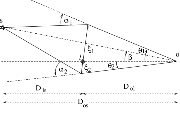
Figure 3: Light ray trajectories in the plane containing the source ($s$), lens ($l$) and observer ($o$), and angular variables and distances relevant for describing the ML event (see text).

Let $\theta_{i}$ ($i=1,2$) be the angles of the two source images with respect to the observer–lens l.o.s., and $\beta$ be the angle to the actual source position. Using that $D_{os}(\theta_{i}-\beta)=D_{ls}\alpha_{i}$, with $\theta_{i}=\xi_{i}/D_{ol}$ and $\alpha_{i}=2R_{S}/\xi_{i}$, it is easy to obtain that

$$\theta_{1,2}={1\over 2}\left[\beta\pm\sqrt{\left({2R_{E}\over D_{ol}}\right)^{2}+\beta^{2}}\;\right],$$ (9)

where the angle $\theta_{2}$ to the fainter image is defined to be negative. The Einstein radius

$$R_{E}\equiv 2\sqrt{GmD_{ol}D_{ls}\over c^{2}D_{os}}$$ (10)

characterizes the size of the impact parameters for which the lensing effect is large, and numerically turns out to be

$$R_{E}=9.0\ {\rm AU}\ \sqrt{{D_{os}\over 10\ {\rm kpc}}{m\over M_{\odot}}x(1-x)},$$ (11)

where from here on we will often use the variable $x\equiv D_{ol}/D_{os}$.

For perfect alignment, $\beta=0$, one has $\theta_{1}=-\theta_{2}=R_{E}/D_{ol}$. Due to the symmetry of this configuration, the image will actually be a ring, the so–called Einstein ring, centered around the source position. Note that $R_{E}$ is just the radius of the projection of this ring onto the lens plane (a plane containing the lens and orthogonal to the l.o.s.).

In general, the angular separation between the two images is

$$\Delta\theta\equiv\theta_{1}-\theta_{2}=\sqrt{\left({2R_{E}\over D_{ol}}\right)^{2}+\beta^{2}}.$$ (12)

For impact parameters smaller than $R_{E}$ one then has

$$\Delta\theta\simeq 1.8\sqrt{{(1-x)\over x}{10\ {\rm kpc}\over D_{os}}{m\over M_{\odot}}}\ {\rm mas}.$$ (13)

This angle is then of order 1 mas (milliarcsec) for ML observations of LMC stars, and $O(\mu$as) for lenses and sources at cosmological distances ($\gg$ Mpc), as in the case of quasar ML by stars in foreground galaxies. Clearly these angular separations are unresolvable with present day telescopes.

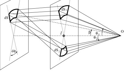
Figure 4: Light ray trajectories from a surface element of the source $dS$. The corresponding surface elements of the two images, projected onto the lens plane, are $dS_{1}$ and $dS_{2}$.

The signal which can however be observed as a result of the ML process is the variation of the intensity of the light source due to the motion of the lensing object with respect to the l.o.s. to the source star. A simple way to compute the resulting amplification of the light of the source is to compare the solid angles subtended by a surface element of the source image ($d\Omega_{i}\equiv dS_{i}/(4\pi D_{ol}^{2})$) with its value ($d\Omega_{0}\equiv dS/(4\pi D_{os}^{2})$) in the absence of lensing effects (see Fig. 4). Since the source flux at the lens plane is constant for the small impact parameters involved, the amplification of the light intensity for each image, $A_{i}$, is just the ratio of these two solid angles. From Fig. 4 we obtain

$$A_{i}={d\Omega_{i}\over d\Omega_{0}}=\left|{\theta_{i}d\phi d\theta_{i}\over\beta d\phi d\beta}\right|.$$ (14)

Substituting $d\theta_{i}/d\beta=(1\pm\beta/\Delta\theta)/2$ (where the $+(-)$ sign is for $i=1(2)$) leads to a total amplification

$$A\equiv A_{1}+A_{2}={1\over 2}\left[{\beta\over\Delta\theta}+{\Delta\theta\over\beta}\right].$$ (15)

Let us define $u\equiv\beta D_{ol}/R_{E}$ as the distance of the lens to the l.o.s. to the star in units of $R_{E}$. We then obtain for the amplification

$$A={u^{2}+2\over u\sqrt{u^{2}+4}}.$$ (16)

Assuming that the lens moves with constant velocity with respect to the l.o.s. during the duration of the ML event, one has

$$u^{2}(t)={b^{2}+[v^{\perp}(t-t_{0})]^{2}\over R_{E}^{2}}\equiv u_{min}^{2}+\left[{(t-t_{0})\over T}\right]^{2},$$ (17)

where $b$ is the minimum distance between the lens trajectory and the l.o.s. to the star, $u_{min}\equiv b/R_{E}$, $t_{0}$ is the time of closest approach and $v^{\perp}$ is the component of the lens velocity relative to the l.o.s. in the direction perpendicular to this same line. The characteristic time

$$T\equiv{R_{E}\over v^{\perp}},$$ (18)

is now usually adopted as the definition of the event duration.

Combining the expression for $u(t)$ with Eq. (16) leads to a time dependent amplification of the luminosity of the source described by a very characteristic light–curve, plotted in Fig. 5 for $u_{min}=1$, 0.5 and 0.2. The amplification reaches its maximum value $A_{max}$ at the time $t_{0}$ as $u(t)$ approaches $u_{min}$. In particular, we have $A_{max}=1.34$ for $u_{min}=1$, and $A_{max}$ diverges (in the point–like source approximation considered in this Section) for $u_{min}\to 0$. The curves are, of course, symmetric about $t_{0}$.

Figure 5: Light–curves, i.e. time evolution of the light amplification, for different values of the normalised impact parameter $u_{min}$.

The event duration $T$ is determined, together with $u_{min}$ (or equivalently $A_{max}$) and $t_{0}$, by fitting the theoretical light–curve to the observed star luminosities plotted as a function of time. There is clearly no useful information contained in $t_{0}$, and the distribution of $A_{max}$ values tests only the expected uniform distribution of impact parameters. The interesting information lies then in the event duration distribution and in the rates of ML events. However, these observables depend in a convoluted way on the lens and source spatial distributions and motions, as well as on the lens mass function, so that it becomes very hard to extract the lens properties in a clean way.

Finally, a crucial characteristic of the ML light–curve is that it should be achromatic, due to the gravitational origin of the lensing effect which causes all wavelengths to be affected equally. This property, and the requirement of having an acceptable fit to the theoretical light–curve, are essential for discriminating the real ML events from other sources of stellar variability.

3.2 Optical depth

A quantity which turns out to be useful in the discussion of ML is the optical depth $\tau$ [95], which is the probability that at a given time a source star is being microlensed with an amplification larger than 1.34, i.e. having $u_{min}<1$.

If we assume for a moment that all the lenses have the same mass $m$, this probability is just the number of lenses inside a tube of radius $R_{E}$ around the l.o.s. to the star, assumed to be at a distance $D_{os}$. The number of objects inside this ‘microlensing tube’ is

$$\tau(D_{os})=\pi\int_{0}^{D_{os}}dD_{ol}{\rho_{l}\over m}R_{E}^{2}={4\pi GD_{os}^{2}\over c^{2}}\int_{0}^{1}dx\ x(1-x)\rho_{l}(x).$$ (19)

Since this expression turns out to be independent of the assumed lens mass, it actually holds also for any arbitrary lens mass distribution.

When performing observations in a given direction, one may have to take into account, especially for bulge observations, that the sources can be distributed with a non–negligible spread along the l.o.s.. In this case, one has to perform an average over the source distribution [96] to obtain the actual optical depth

$$\tau={1\over N_{s}}\int dD_{os}{dn_{s}\over dD_{os}}\tau(D_{os}),$$ (20)

where the normalization factor is $N_{s}=\int dD_{os}dn_{s}/dD_{os}$ and $dn_{s}/dD_{os}$ describes the number density profile of detectable sources along the l.o.s.. For observations in the bulge, it can be parameterised as $dn_{s}/dD_{os}\propto\rho_{s}D_{os}^{2-2\beta}$. The factor $D_{os}^{2}$ is due to the change of the volume element with distance. The parameter $\beta$ arises because the observations are magnitude limited, and the fraction of sources with luminosities larger than $L$ is assumed to scale as $L^{-\beta}$, implying that the fraction of stars which remain detectable behave as $D_{os}^{-2\beta}$. Hence,

$$\tau={\int dD_{os}\ D_{os}^{2(1-\beta)}\rho_{s}\tau(D_{os})\over\int dD_{os}\ D_{os}^{2(1-\beta)}\rho_{s}}.$$ (21)

A reasonable range for $\beta$ has been estimated to be $\beta=1\pm 0.5$ in Baade’s Window [89], and we will generally use $\beta=1$ in the discussion of ML in the bulge.

3.3 Event duration distribution

Due to its simplicity and the property of being independent of the lens motion and mass distribution, the optical depth is often used in discussions of the ML observations. However, since the experiments measure the number of events and their durations, a more useful quantity is the ML rate, and in particular its distribution as a function of the event durations. This distribution contains all the information related to the ML process.

To obtain the event duration distribution, we start from the expression for the differential rate in terms of the variables depicted in Fig. 6. The rate of events with amplification $A_{max}$ above a certain threshold $A_{th}$, i.e. with $u_{min}<u_{th}$, is the flux of lenses inside a microlensing tube of radius $u_{th}R_{E}$ around the l.o.s. to the star. One then has

$${d\Gamma\over dm}={dn\over dm}v^{\perp}\cos\omega f({\bf v}^{\perp})d^{2}{\bf v}^{\perp}dS,$$ (22)

where $dn/dm$ is the lens mass function, $dS=u_{th}R_{E}d\alpha dD_{ol}$ is a surface element of the ML tube, $\omega$ is the angle between the normal to the surface element and the lens relative velocity vector ${\bf v}^{\perp}$ (orthogonal to the l.o.s.). From here onwards we will adopt $u_{th}=1$, since it is enough to recall that the rates are just proportional to $u_{th}$. The function $f$ in Eq. (22) describes the distribution of relative velocities. Due to the motion of the observer and the source, with velocities ${\bf v}_{o}$ and ${\bf v}_{s}$ respectively, the ML tube will be moving with a speed

$${\bf v}_{t}=x{\bf v}_{s}+(1-x){\bf v}_{o}.$$ (23)

If ${\bf v}_{l}$ is the lens velocity in the same reference frame, the lens relative velocity with respect to the ML tube is

$${\bf v}={\bf v}_{l}-{\bf v}_{t}.$$ (24)

It is convenient to decompose all velocities as ${\bf v}_{x}={\bf v}_{x,bulk}+{\bf v}_{x,dis}$, where ${\bf v}_{x,bulk}$ accounts for a bulk global motion and ${\bf v}_{x,dis}$ is a dispersive contribution, which will be assumed to be Gaussian distributed. From the previous expressions we then have

$${\bf v}_{bulk} = {\bf v}_{l,bulk}-x{\bf v}_{s,bulk}-(1-x){\bf v}_{o}$$

$${\bf v}_{dis} = {\bf v}_{l,dis}-x{\bf v}_{s,dis}.$$ (25)

Figure 6: ML tube section in a plane orthogonal to the l.o.s. to the star. The tube radius is $u_{th}R_{E}$, and we show the angular variables entering the computation of the flux of lenses (moving with relative velocity $v^{\perp}$ in this plane) through this tube.

The orthogonal component of ${\bf v}$ can be projected onto axes along the directions of increasing longitudes, $\hat{\ell}$, and latitudes, $\hat{b}$, i.e. ${\bf v}^{\perp}=v^{\ell}\hat{\ell}+v^{b}\hat{b}$. The velocity distribution function can then be obtained from the assumed Gaussian distribution $G(v^{i}_{dis})$ of the dispersive components ($i=\ell,b$)

$$G(v_{dis}^{i})={1\over\sqrt{2\pi}\sigma^{i}}{\rm exp}\left[-{(v_{dis}^{i})^{2}\over 2(\sigma^{i})^{2}}\right],$$ (26)

where $\sigma^{i}$ are the corresponding velocity dispersions. If both lenses and sources have non–vanishing dispersions, $\sigma^{i}_{l}$ and $\sigma^{i}_{s}$ respectively, the relative velocity dispersion is just the quadratic sum (see Eq. (25))

$$\sigma^{i}=\sqrt{(\sigma^{i}_{l})^{2}+(x\sigma^{i}_{s})^{2}}.$$ (27)

In terms of the modulus of the orthogonal relative velocity $v^{\perp}$, which is the quantity related to the event duration $T=R_{E}/v^{\perp}$, we can write (see Fig. 6)

$$v_{dis}^{\ell} = -v_{bulk}^{\ell}-v^{\perp}\cos\gamma$$

$$v_{dis}^{b} = -v_{bulk}^{b}-v^{\perp}\sin\gamma,$$ (28)

where $\gamma\equiv\omega+\alpha$. We can now substitute in Eq. (22)

$$f({\bf v}^{\perp})d^{2}{\bf v}^{\perp}=G(v_{dis}^{\ell})G(v_{dis}^{b})dv_{dis}^{\ell}dv_{dis}^{b},$$ (29)

and use that $d^{2}{\bf v}^{\perp}=v^{\perp}dv^{\perp}d\omega$, to end up with

$${d\Gamma\over dm}={dn\over dm}R_{E}(v^{\perp})^{2}\cos\omega G(v_{dis}^{\ell})G(v_{dis}^{b})dv^{\perp}d\omega d\gamma dD_{ol}.$$ (30)

The integral in $\omega\in[-\pi/2,\pi/2]$ (only lenses entering the ML tube) is now trivial. The distribution in terms of the event duration $T=R_{E}/v^{\perp}$ is then

$${d\Gamma\over dTdm}=2\int_{0}^{2\pi}d\gamma\int_{0}^{D_{os}}dD_{ol}{dn\over dm}\left({R_{E}\over T}\right)^{4}G(v_{dis}^{\ell})G(v_{dis}^{b}).$$ (31)

The expression for the differential rate obtained here is quite general, including an arbitrary lens mass function, the effect of bulk velocities of observer, lens and source as well as the (eventually anisotropic) velocity dispersions of lenses and sources. In order to apply it to a particular observational case, one needs just to construct the appropiate $G(v^{i}_{dis})$ using Eqs. (26), (27) and (28), with the replacement $v^{\perp}=R_{E}/T$. The source velocity dispersion is important for bulge observations, but can be neglected for LMC stars lensed by Galactic objects. In this last case, a further integral can be performed analytically if the lens dispersion is isotropic [92, 74]. The effect of the bulk motions is small for lensing of LMC stars by halo objects [92], but becomes important when considering the rotating disk populations or for the discussion of bulge observations.

If the spread in source distances is non–negligible, an average over the source locations similar to the one in Eq. (21) should also be performed.

3.4 Mass functions and time moments

The determination of the lens mass function $dn(x)/dm$ is one of the main purposes of ML observations. Very little is known about it a priori. A usual assumption regarding its spatial dependence is the so–called factorization hypothesis, i.e. that the mass function only changes with position by an overall normalization

$${dn(x)\over dm}={\rho(x)\over\rho_{0}}{dn_{0}\over dm},$$ (32)

where the subscript 0 stands for the local value of the lens densities. We note that this may not be necessarily a good approximation, since even for a single Galactic component, e.g. the disk, the star formation conditions are quite different in the high density regions close to the bulge from those in the low density regions in the outskirts of the disk. One should also keep in mind that the mass functions of stars in different Galactic components are not expected to be at all similar. In fact, already the measured spheroid star mass function [73, 97] is completely different from the disk one [63].

It is often useful to discuss ML predictions under the simplifying assumption of having a common lens mass $M$ as a first step, so that

$${dn\over dm}={\rho\over m}\delta(m-M).$$ (33)

In this case, one has then

$${d\Gamma\over dT}={2\over M}\int_{0}^{2\pi}d\gamma\int_{0}^{D_{os}}dD_{ol}\rho_{l}(D_{ol})(v^{\perp})^{4}G(v_{dis}^{\ell})G(v_{dis}^{b}).$$ (34)

Since $T$ only enters in this equation through $v^{\perp}\propto\sqrt{M}/T$, it is easy to see that the differential rate distributions for two lens models with masses $M_{1}$ and $M_{2}$ are related through

$${d\Gamma\over dT}(T_{1},M_{1})={M_{2}\over M_{1}}{d\Gamma\over dT}(T_{2}=T_{1}\sqrt{M_{2}/M_{1}},M_{2}).$$ (35)

This implies that the total ‘theoretical’ rate

$$\Gamma_{th}=\int_{0}^{\infty}dT{d\Gamma\over dT}$$ (36)

scales with the assumed lens mass as

$$\Gamma_{th}\propto 1/\sqrt{M}.$$ (37)

In order to actually predict the total event rate for a given experiment, one has to take into account that the observational efficiencies are generally smaller than unity and, moreover, that they are a function of the event duration, mainly due to the poor sampling of the short duration events and the incomplete coverage of the very long duration ones. Hence, the predicted total rate for a given experiment is a convolution of the differential rate with the experimental efficiency $\epsilon(T)$, i.e.

$$\Gamma=\int_{0}^{\infty}dT\epsilon(T){d\Gamma\over dT}.$$ (38)

The efficiency $\epsilon(T)$ actually also takes into account the fact that the observational threshold could be different from $A_{max}>1.34$, so that in Eq. (38) the differential rate should be computed with $u_{th}=1$.

Other quantities which turn out to be useful are the expected time moments

$$\langle T^{n}\rangle={1\over\Gamma}\int_{0}^{\infty}dT\epsilon(T){d\Gamma\over dT}T^{n},$$ (39)

where $n=1$ gives just the average event duration $\langle T\rangle$.

One may relate these time moments with the moments of the mass distribution [93, 98], so that once the responsible lens population is identified, its mass distribution may be reconstructed, in the sense of knowing its moments, from the observed time moments. A more elementary method for reconstructing the mass distribution is to use just an ansatz, depending on few parameters, to describe a family of possible mass functions (e.g. power–law or Gaussian mass functions), and use a likelihood method to determine these parameters from a fit to the observed event durations [88, 89, 90].

A useful relation expressing the fact that the probability of ML $\tau$ is just proportional to the total rate times the average event duration (computed with unit efficiency), is

$$\Gamma_{th}={2\over\pi}{\tau\over\langle T\rangle_{th}},$$ (40)

with the geometrical factor $2/\pi$ being related to the particular definition of event duration adopted.

Figure 7: Differential rate distribution for LMC stars lensed by a standard halo population consisting of objects with a common mass of $M=0.01M_{\odot}$ (solid line) and $M=0.1M_{\odot}$ (dashed line).

From this relation it is also clear that, in the case in which the lenses are assumed to have a common mass $M$, the average event duration scales with $M$ as

$$\langle T\rangle_{th}\propto\sqrt{M},$$ (41)

just due to the fact that the associated Einstein radii scale as $\sqrt{M}$. As an example of the expectations for the ML observations, Fig. 7 shows the predicted differential rate for LMC stars lensed by objects in a standard Galactic halo, assuming two different common lens masses, $10^{-2}M_{\odot}$ (solid lines) and $10^{-1}M_{\odot}$ (dashed lines). The behaviour mentioned in Eq. (35) is clearly apparent, and it is important to notice that the distributions have a significant spread in the event durations, which is even larger if one allows for a distribution in the lens masses using a non–trivial mass function. This shows the difficulties underlying the determination of the responsible lens masses from the observation of the event durations.

Another quantity useful for characterizing the theoretical models of lensing populations is the average observer–lens distance, which is just

$$\langle D_{ol}\rangle\equiv{1\over\Gamma_{th}}\int_{0}^{D_{os}}dD_{ol}{d\Gamma\over dD_{ol}}D_{ol},$$ (42)

eventually also averaged over the source spatial distribution.

4 Microlensing searches

In this Section we discuss the ongoing searches for ML events in directions towards the LMC and the bulge, and the possible interpretations of the first results obtained.

4.1 Microlensing signatures

The main difficulty that ML searches have to face is the very small probability of occurrence of events with observable amplifications. For example, if the halo, distributed according to Eq. (1), wholly consists of compact objects capable of producing ML events, the resulting optical depth for ML of LMC stars is $\tau_{halo}\simeq 5\times 10^{-7}$. On the other hand, since the velocity dispersion of halo objects is $\sigma\simeq v_{c}/\sqrt{2}$, an estimate of the typical event duration is $T\simeq R_{E}/\sigma\simeq 100\ {\rm days}\sqrt{m/M_{\odot}}$ (taking $x\simeq 1/4$ in Eq. (10)). Hence, for lenses with masses in the range $10^{-2}$–$10M_{\odot}$, the characteristic event duration will be between a week and a year. Several million stars should then be monitored for more than a year to get a handful of events in this case. For the lower end of the interesting mass range, $10^{-7}$–$10^{-4}M_{\odot}$, the events last less than a day, and the event rates, $\Gamma\propto\tau/\langle T\rangle$, are much larger. To be sensitive to this mass range, fewer stars need to be followed but with a much better time coverage, i.e. performing several measurements per night. Both strategies have actually been employed in order to explore the whole range $10^{-7}<m/M_{\odot}<1$. The computation of the optical depth for bulge stars, lensed by low mass stars in the bulge and disk, also leads to $\tau\simeq 10^{-6}$, with typical event durations of a few weeks (see below), so that in this case also several million stars need to be monitored for more than a year to get significant statistics.

In addition to the small number of expected events, a further complication is that there is a large background of variable stars, and special care should be taken in order to avoid including one of these stars as an ML event. Variable stars represent a fraction $\sim 3\times 10^{-3}$ of the total number of stars, and an interesting byproduct of the ML searches has been the compilation of the more complete catalogs of variables in the LMC [99, 100, 101] and in Baade’s window [102].

There are many signatures which allow one to distinguish between intrinsic stellar variabilities and ML events, so that one can be confident that a real signal of ML is found:

• Most variables are periodic, while due to the very small probability for a star to be lensed, ML events should never repeat for the same star.

• Most intrinsic luminosity variations have an associated change in the star temperature, so that the variation is color dependent. ML events are instead achromatic, due to their gravitational nature (unless there is blending of two sources with significantly different colors).

• Most variable stars produce pulses which are asymmetric in time, with a rapid rise and a slower decline of the star luminosity, while ML events are time symmetric.

• The light–curves of real ML events should be reasonably fitted by the theoretical light–curve, Eq. (16), eventually allowing for stellar blending or for peculiarities such as lens or source binarity, finite source size or the non–uniform motion of the Earth (see Section 5).

Figure 8: Gold–plated event obtained by the MACHO collaboration in their LMC analysis.

These general features can be seen for instance in Fig. 8, which shows the light–curve of the first ML event observed by the MACHO collaboration in the LMC (from Ref. [20]). The light–curves in the two colors are reasonably well fitted by the theoretical curve, and the ratio of the amplifications in each color (lower panel) is well consistent with an achromatic signal. Accurate testing of the achromaticity, and even of the stability of the source spectrum [104], during the ML event is now possible with the Early Warning systems implemented both by the MACHO [105] and OGLE [106] collaborations. This allows one to know the existence of an ongoing ML event in real time, as the amplification is starting to grow, and hence to study the source properties with other bigger telescopes and to organize intense follow–up studies of the light–curves with telescope networks around the globe [105].

In addition to the above mentioned features, ML events should have the following statistical properties:

• Unlike star variability, ML events should happen with the same probability for any kind of star, and this should reflect in the distribution of ML events in the color magnitude diagrams.

• The distribution of $A_{max}$ values should be the one corresponding to a uniform distribution of $u_{min}$.

• The distribution of $A_{max}$ and $T$ values should be uncorrelated (once the effects of blending are taken into account [103]).

Due to the large number of stars that need to be followed to observe ML events, the ongoing searches have focused on two targets: $i)$ Stars in the Large and Small Magellanic Clouds, which are the nearest galaxies having l.o.s. which go out of the Galactic plane and well across the halo. $ii)$ Stars in the Galactic bulge, which allow one to test the distribution of lenses near to the plane of the Galaxy.

Globular Clusters, having less than $10^{5}$ stars, could only be useful for testing lens masses below Jupiter’s mass, although it has been pointed out that they could provide an interesting lensing population, using some clusters which are in the front of the bulge or SMC fields [107, 108]. On the other hand, observations of ML of stars in the Andromeda galaxy (M31) are starting to be performed, but since M31 is much further away ($D_{os}\simeq 770$ kpc), the severe crowding of stars requires the use of ‘pixel’ lensing, since the individual stars cannot be resolved (see Section 6).

4.2 Searches towards the Magellanic Clouds

4.2.1 Experimental results

Two experiments are now looking for ML in the Magellanic Clouds. The first is the French EROS (Expérience de Recherche d’Objets Sombres) experiment, which actually had two different programs at La Silla Observatory in Chile: $i)$ they have used a CCD camera in a 40 cm dedicated telescope to make short exposures (10 min each) so as to be able to test short duration events; $ii)$ they have analysed plates from a 1 m Schmidt telescope, which made two exposures per night in different colors, from which they have followed the light–curves of several million stars since 1991. They have also one year of data from the SMC yet to be analysed. From 1996, they plan to start observations with a new dedicated 1 m telescope, equipped with two CCD cameras, and this will improve their statistics significantly.

The second is the MACHO (Massive Compact Halo Objects) experiment , an Australian/American collaboration using a 1.3 m dedicated telescope at the Mount Stromlo Observatory in Australia. They can simultaneously take images in a ‘red’ and a ‘blue’ band using two CCD cameras. They have measured the light–curves of $\sim 10^{7}$ stars in the LMC since 1992, and they also have measurements in the SMC, though with poorer statistics.

The EROS group has found no events in their CCD search, after looking at the light curves of 82000 stars during 10 months [109]. In the first three years of Schmidt plate data [110], with a total exposure $E=3\ {\rm yr}\times 3.33\ 10^{6}$ stars, they found two candidate ML events, with durations $T_{1}=23$ d and $T_{2}=29$ days. From the two events found, and their efficiency $\epsilon(T)$, they estimate an optical depth towards the LMC of

$$\tau^{EROS}_{est}\equiv{\pi\over 2E}\sum_{events}{T_{i}\over\epsilon(T_{i})}=8.2\times 10^{-8}.$$ (43)

The analysis of the first year of MACHO observations [103], using 9.5 million light–curves, revealed the presence of three ML events, with durations $T=19.4$, 10.1 and 15.6 d (see Note added). Performing a likelihood analysis, they inferred from these events an optical depth towards the LMC

$$\tau^{MACHO}=8.8^{+7}_{-5}\times 10^{-8}.$$ (44)

An estimate of the optical depth as in Eq. (43) would have lead to $\tau_{est}^{MACHO}=8\times 10^{-8}$, in good agreement with the maximum likelihood estimate.

The values of $\tau$, Eqs. (43) and (44), should however be taken cum grano salis since, for instance, lenses with masses larger than 0.1 $M_{\odot}$, to which the experiments are not very sensitive yet, could in principle contribute significantly to $\tau$. On the other hand, if some of the events are not due to real ML, the optical depth could be smaller. Also, it has been noted [112] that the error associated with $\tau$ is larger than the naive Poissonian estimate, due to the wide range of expected timescales. As a result, it is always convenient to confront directly the expected event rates and durations, although this requires particular assumptions concerning the lens mass function.

Lensing	$\tau$	$\Gamma_{th}$	$\langle T\rangle_{th}$	$\langle D_{ol}\rangle$
component	[$10^{-7}$]	[$(10^{7}$ stars yr)-1]	[days]	[kpc]
Halo	5.4	$89/\sqrt{m_{0.05}}$	$14\sqrt{m_{0.05}}$	14
Spheroid	0.44$\rho^{S}_{*}$	$6.7\rho^{S}_{*}/\sqrt{m_{0.05}}$	$15\sqrt{m_{0.05}}$	9.0
Thick disk	$0.47\Sigma_{45}$	$5.5\Sigma_{45}/\sqrt{m_{0.05}}$	$20\sqrt{m_{0.05}}$	3.6
Thin disk	$0.11\Sigma_{30}$	$1.1\Sigma_{30}/\sqrt{m_{0.05}}$	$23\sqrt{m_{0.05}}$	1.1

Table 1: Predicted optical depth $\tau$, theoretical ($\epsilon=1$) rates $\Gamma_{th}$, average event duration $\langle T\rangle_{th}$ and average lens distance $\langle D_{ol}\rangle$, for ML of LMC stars by different Galactic lensing populations: a standard halo, a heavy spheroid (where $\rho^{S}_{*}\equiv\rho^{S}_{0}/0.0015M_{\odot}$ pc^-3), a dark thick disk (with $\Sigma_{45}\equiv\Sigma_{0}/(45M_{\odot}$ pc^-2) and thin disk (with $\Sigma_{30}\equiv\Sigma_{0}/(30M_{\odot}$ pc^-2).

In Table 1 we give the values for $\tau$, $\Gamma_{th}$, $\langle T\rangle_{th}$ and $\langle D_{ol}\rangle$ for observations towards the LMC, for the different dark lensing components discussed in Section 2. The theoretical rates and average durations in the Table are computed assuming a common lens mass and unit efficiency, while the actual efficiencies of the experiments are typically $\leq 30$% and $T$ dependent [103, 110]. In any case, taking into account the efficiencies would lead to more than 10 expected events in any of the searches sensitive to long duration events, arising from a standard halo model wholly consisting of objects with masses between $10^{-4}$ and $10^{-1}M_{\odot}$ [110, 103]. In the EROS CCD search, more than 2.3 events (the 90% CL upper bound corresponding to no observed events) would be expected from a standard halo composed of objects with $5\times 10^{-8}<m/M_{\odot}<7\times 10^{-4}$ [109].

Figure 9: LMC bounds from EROS results. The upper panel shows the expected number of events for the two EROS searches from a standard halo wholly composed of compact objects as a function of their assumed common mass. The lower panel shows the corresponding 95% CL bounds on the halo mass contained within 50 kpc, or alternatively (right scale) the allowed fraction of compact objects in a standard halo. Also the bounds from the first year LMC MACHO results are shown.

From these results it is possible to set an upper bound on the contribution to the halo mass coming from objects with masses in the range $5\times 10^{-8}<m/M_{\odot}<1$, which is shown in Fig. 9, taken from Ref. [110]. The upper panel shows the expected number of events in the two EROS experiments for halo models in which all lenses are assumed to have the same mass. The lower panel gives the resulting 95% CL constraints on the halo mass within 50 kpc, or alternatively (right scale) the fraction $f$ of the mass of a standard halo which is allowed to consist of compact objects. The thick line is the combined EROS result, while the thin line is the MACHO excluded region. From this we see that in the wide range $10^{-7}<m/M_{\odot}<10^{-1}$, the halo fraction should be less than 30%. This last result is also independent of the assumption that the lenses have a common mass, as long as all the masses are inside that range. Although the value of this fraction depends strongly on the reference halo model adopted, the bound on the halo mass (left scale) is quite insensitive to this, providing then a more solid result [113, 103, 87].

It is also possible to estimate the lens masses which are more likely to produce the observed event durations. Since the durations observed actually have a narrow dispersion, it is reasonable to compare with models having a common lens mass, since an extended mass function would only increase the spread in the expected event durations. From a maximum likelihood fit, the MACHO group [103] finds that for the standard halo, the more likely lens masses turn out to be in the range $m=0.065^{+0.06}_{-0.03}M_{\odot}$ (68% CL), which correspond to brown dwarfs or, in the upper side, to very faint stars. The EROS group [110], which observed somewhat larger durations, infer a ‘95% CL’ interval [0.01–0.7$]M_{\odot}$ from the $T=23$ d event, while an allowed mass interval of [0.02–1.1$]M_{\odot}$ from the $T=29$ d event.

4.2.2 Interpreting the observations

The results discussed in the last Section indicate that the observed ML rates and optical depths towards the LMC are significantly smaller than those expected from a standard halo consisting entirely of compact objects with masses in the range $10^{-7}$–$10^{-1}M_{\odot}$ (see Note added). However, they are larger than those that would result from the known populations of faint stars in the Galactic disk, which lead to $\tau\sim 10^{-8}$ [66], and from those in the LMC itself, which lead to a prediction $\tau\leq 3\times 10^{-8}$ [114, 94, 103].

Several possible scenarios have been suggested to account for these observations, which we now discuss:

• The halo consists of a fraction $f\simeq 0.1$–0.3 of compact baryonic objects [103, 115, 110, 116, 117, 118], with the remaining 70–90% being either in cold baryonic gas [49, 50, 51], which does not produce any lensing effect (see however [119]), or in white dwarfs and neutron star stellar remnants or heavy black holes, to which the present searches are almost insensitive, or alternatively in non–baryonic forms.

• The halo may actually be much lighter than the reference models usually considered. Varying the halo models so as to allow for declining rotation curves or a maximum contribution to $v_{c}$ from the Galactic disk, can result in models with much larger allowed mass fraction in compact objects, $f\geq 0.5$ [120, 113, 103, 87, 121]. Fractions $f\simeq 1$ may even be consistent with the ML results, although they seem disfavoured when combined with other Galactic dynamical constraints [87]. Allowing for anisotropic velocity distributions can further affect, in a sizeable way, the rates and event durations [122, 123]. For instance, a tangentially anisotropic velocity distribution leads to a rate which is a factor of two larger than the one resulting from a radially anisotropic distribution, with the isotropic distribution usually adopted giving an intermediate value. Allowing for halo flattening does not modify sizeably the predictions for LMC observations [124], due to a compensation between the increase in the local halo density required to keep unchanged the rotation velocity and the fact that the lenses become closer on average. Tilting a flattened halo may however have some effects [125]. The effects of prolate halos were discussed in Ref. [126], and they may reduce the optical depth by up to 35%, although prolate shapes seem unnatural.

  One must also mention that some observations suggest that the LMC has a dark halo [127, 128] and, of course, if the Milky Way halo consists of compact baryonic objects the LMC one should also consist of similar objects. In this case the contribution of the LMC halo to the optical depth is $\sim 20$% of that of a standard Galactic halo [129, 114, 94], and hence is already comparable with the observed depth. Its inclusion would then further increase the gap between the observations and the theoretical halo model predictions.

• The halo may be completely non–baryonic, i.e. $f=0$, with the observed events being due to dark objects in the Galactic spheroid [74] or in the Galactic thick disk [65, 66]. From Table 1 we see that, if the density of the outer–spheroid is similar to that of the heavy spheroid models [33, 71], or if the local column density of the thick disk is close to its upper bound $\Sigma\simeq 45M_{\odot}/$pc³ (see Section 2), these models give results which are consistent with the observations. The inferred lens masses for these models are similar to those inferred for the halo case, since the slower motions are compensated by the fact that the lenses are typically closer, having then smaller associated Einstein radii [66, 94]. The additional contribution arising from the faint stars in the Galactic thin disk and in the LMC itself plays a non–negligible role in these scenarios.

• It has been proposed [130] that the contribution from LMC stars may be enough to explain the observations. In Ref. [130], an optical depth $\tau\simeq 5\times 10^{-8}$ is obtained for this contribution, assuming that the LMC bar is quite massive. Other estimates of the optical depth of stellar LMC populations lead however to smaller values [114, 131, 94], and the estimated event durations for lensing by faint stars in the LMC are somewhat larger than the observed ones [94, 103]. Another difficulty with this interpretation is that the two EROS events are actually outside the LMC bar, in a region where the LMC stars should contribute negligibly to the optical depth, but it could still be allowed if one considers that some of the events may not actually be due to ML.

In order to distinguish among these alternative scenarios, clearly more statistics are required. The main tests that will clarify the situation are the following:

• If the lenses are Galactic, rather than in the LMC, the optical depth should be independent of the location of the source star in the LMC. Hence, a strong variation of $\tau$ across the LMC will be a clear signal that the lenses are in the LMC itself.

• The Einstein radius of a lens projected onto the source plane is

  $${R_{E}\over x}\simeq 4.3\times 10^{3}R_{\odot}\sqrt{\left({m\over M_{\odot}}\right)\left({1-x\over x}\right)}.$$ (45)

  Hence, if the lens is a star in the LMC, i.e. $1-x\leq 10^{-2}$ and $m\geq 0.1M_{\odot}$, this quantity is comparable with the size of a red giant star. It then becomes more likely to observe deviations in the light–curve due to the finite source size (see Section 5). For Galactic lenses, the projected radius is much larger, making the observation of such effects very unlikely.

To discriminate between Galactic lenses in the thick disk or in the spheroid looks particularly difficult, since they lead to similar predictions for the LMC rates and average event durations (see Table 1). Some strategies have been proposed to study this issue:

• If sufficient data are gathered from the SMC, the ratio between the rates obtained for the SMC and the LMC should be quite different in the two scenarios. Since the SMC is at a smaller angle with respect to the Galactic center than the LMC, but however at larger latitudes, one has $\Gamma_{SMC}/\Gamma_{LMC}\simeq 1.7$ for the spheroid lenses, while $\Gamma_{SMC}/\Gamma_{LMC}\simeq 0.9$ for the thick disk [94]. Of course, this assumes a negligible contribution from lensing populations in the Magellanic Clouds themselves. The comparison of LMC and SMC rates was originally proposed as a tool to study the ellipticity of the Galactic halo [124], and then suggested as a way to distinguish between the thick disk and the halo [66].

• Since thick disk objects have small velocity dispersion ($\sim 40$ km/s) and a global rotational motion, thick disk lenses cross the l.o.s. to LMC stars at an approximately constant speed (for a given value of $x$). This implies that the event duration distribution due to thick disk lenses has a smaller dispersion, $\Delta T\equiv\sqrt{\langle T^{2}\rangle-\langle T\rangle^{2}}/\langle T\rangle$, than the spheroid or halo ones. This difference is still present if one takes into account the spread in $T$ due to the ignorance of the lens mass function, as long as lens masses heavier than the Jeans mass $\simeq 7\times 10^{-3}M_{\odot}$ are considered [94]. Hence, with several dozens of events this test may become useful.

• Lenses belonging to the Galactic disk populations, which are on average closer to the observer (see Table 1), may lead to parallax effects due to the motion of the Earth around the Sun (see Section 5). This parallax may be observable for most of the thin disk events, and for around 15% of the thick disk ones [66].

4.3 Searches towards the bulge

4.3.1 Experimental results

Three experiments are looking for ML towards the Galactic center, and they have obtained a large number of ML events, well above the initial expectations. The OGLE (Optical Gravitational Lensing Experiment) experiment is a collaboration between Warsaw and the Carnegie Institute, using a 1 m telescope with a CCD camera at Las Campanas Observatory, Chile. Its main purpose is the study of ML and variable stars in the Galactic bulge, where they have monitored $\sim 10^{6}$ stars since 1992. Most of the exposures are taken in the $I$ band, and fewer $V$ band pictures are taken to check the achromaticity. The MACHO collaboration also looks at fields in the bulge, especially when the LMC is low in the sky. They have followed more than $10^{7}$ stars since 1993. The DUO (Disk Unseen Objects) experiment is a French collaboration which has analysed Schmidt plates taken (two in red and one in blue per night) at the ESO 1 m telescope at La Silla, Chile, since 1994 [132]. They have found a dozen events, but the analysis is not yet available.

The analysis of the first two years of OGLE data [133] provided 9 events, with 8.6 d$<T<62$ d, including a binary lens candidate, out of $10^{6}$ light–curves of stars in Baade’s Window and in other fields at $\ell=\pm 5^{\circ}$ and $b=-3.5^{\circ}$. The distribution of peak amplifications is consistent with ML expectations and the lensed stars are scattered in the color–magnitude diagrams as if taken at random from the overall distribution of bulge stars. From these results they estimate an average optical depth for bulge sources of

$$\tau^{OGLE}=(3.3\pm 1.2)\times 10^{-6}.$$ (46)

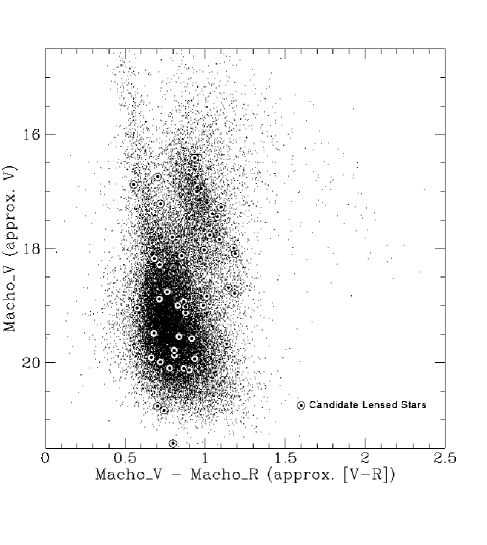
Figure 10: Color–Magnitude diagram of a sample of the stars monitored in the bulge by the MACHO collaboration showing with circles the location of the first 45 bulge ML events, reprinted with permission from The Astrophysical Journal.

The searches of the MACHO collaboration have returned 45 ML events towards the bulge in their first year, looking at several fields with $0^{\circ}<\ell<7^{\circ}$ and $-2^{\circ}>b>-6^{\circ}$ [134, 135], and there are already more than 40 events seen in the 1995 season. The observed event durations range from 4.5 d to 110 d. An analysis based on 13 events detected among $1.3\times 10^{6}$ clump giant stars, in fields centered at $\ell=2.5^{\circ}$ and $b=-3.6^{\circ}$, leads to an estimated average optical depth [135]

$$\tau^{MACHO}=3.9^{+1.8}_{-1.2}\times 10^{-6}.$$ (47)

The color–magnitude diagram for the first 45 candidate ML events (from Ref. [135]) is shown in Fig. 10. The red clump stars are centered at $V\simeq 17$ and $V-R\simeq 1$. The events are distributed all over the diagram. The comparatively large fraction of lensed stars for $V<19$ is partly due to the larger ML efficiency associated with the brightest stars, although there are suggestions [135] that the optical depth is smaller on the average than the result in Eq. (47) associated with the red clumps. This could be related to the fact that a fraction of the sources are foreground disk stars, having then smaller associated optical depth, and this fraction is minimized in the red clump subsample. Also, since red clumps are very bright stars, they can be seen further away than main sequence stars ($\beta\simeq 0$ in Eq. (20)) and hence are more likely to be lensed. The effect of disk lenses and sources should be enhanced at smaller latitudes and at larger longitudes, hence the relevance of gathering events in several fields so as to be able to map the ML rates in different directions and from this infer which are the populations responsible for the observations. There are, in fact, preliminary indications that the optical depth increases at smaller latitudes [135].

4.3.2 Interpreting the observations

The ML searches towards the bulge were initially believed to be sensitive mainly to disk lenses, and in this sense these observations, unlike the LMC ones, were warranted to provide events independently of the existence of compact objects in the halo. The optical depth for bulge stars lensed by faint disk stars was expected to be $\leq 10^{-6}$ [19, 18], as shown in the row labeled ‘faint stars’ in Table 2, which was computed by Griest et al. [19] assuming a fixed local number density of disk stars and allowing their mass function to vary consistently with the errors in its determination. The contribution of the dark halo was not expected to be dominant, although the predictions depend sensitively on the assumed halo core radius $a$, increasing with decreasing $a$, and they also increase with the halo flattening [87]. It was then shown [74] that in the heavy spheroid models the contribution of spheroid lenses was comparable to that of disk lenses, and arose mainly from the inner 2 kpc of the Galaxy [136], where this component describes the bulge. However, the associated event durations were typically smaller than the disk ones. Kiraga and Paczyński [96] studied the bulge–bulge ML with Kent’s axisymmetric model, showing also the importance of averaging over the source distribution (Eq. (21)), since this increases both the bulge–bulge rates and the average event durations by $\sim 25$% (increasing $\tau$ by $\sim 50$%). This averaging however does not significantly change the rates due to disk lenses, because these are on average more distant from the sources and less centrally concentrated than the bulge lenses. They also considered how the rates due to disk lenses are reduced in models where a ‘hole’ in the central distribution of disk stars is present (see Section 2.4). To illustrate this last point, we show in Table 2 the predictions for a disk with a hole in the inner 2.5 kpc (i.e. considering only $D_{ol}<6$ kpc), as well as those for a disk without a hole. Finally, they also discussed the dependence of the predictions on the parameter $\beta$ (see Eq. (20)) describing the change with distance of the fraction of sources which remain observable.

Lensing	$\tau$	$\Gamma_{th}$	$\langle T\rangle_{th}$	$\langle D_{os}\rangle$
component	[$10^{-6}$]	[$(10^{6}$ stars yr)-1]	[days]	[kpc]
Faint stars	0.29–0.96	2.2–7.5	$\sim 30$	5.7
Bar($\alpha=10^{\circ}$)	$1.74\ M_{2}$	$19\ M_{2}/\sqrt{m_{0.2}}$	$20\sqrt{m_{0.2}}$	7.0
Bar$(\alpha=30^{\circ}$)	$0.97\ M_{2}$	$12\ M_{2}/\sqrt{m_{0.2}}$	$18\sqrt{m_{0.2}}$	7.4
Disk($D_{ol}<12$)	$0.42\ \Sigma_{30}$	$4.3\ \Sigma_{30}/\sqrt{m_{0.2}}$	$22\sqrt{m_{0.2}}$	5.5
Disk($D_{ol}<6$)	$0.31\ \Sigma_{30}$	$2.5\ \Sigma_{30}/\sqrt{m_{0.2}}$	$28\sqrt{m_{0.2}}$	4.1
Thick disk	$0.37\ \Sigma_{45}$	$3.3\ \Sigma_{45}/\sqrt{m_{0.2}}$	$25\sqrt{m_{0.2}}$	6.2
Spheroid	$0.72\rho^{S}_{*}$	$14\rho^{S}_{*}/\sqrt{m_{0.2}}$	$12\sqrt{m_{0.2}}$	7.7
Halo	0.24	$4.7/\sqrt{m_{0.2}}$	$12\sqrt{m_{0.2}}$	5.4

Table 2: Predicted optical depth $\tau$, ‘theoretical’ rates $\Gamma_{th}$, average event duration $\langle T\rangle_{th}$ and lens distance $\langle D_{ol}\rangle$, for ML of stars in Baade’s window by different lens populations (see text and caption of Table 1). For the disk and halo predictions we assumed the sources to be in the bar.

Since the observed optical depth, Eqs. (46) and (47), is above the expectations from all these models, it was suggested that the cause of these large rates could be the fact that the bulge is actually triaxial, with the larger axis making a small angle with respect to the l.o.s. [96, 137]. In this way, the average distance between sources and lenses is larger, with a corresponding increase of the associated Einstein radii, and also the l.o.s. to a source goes through a larger number of lenses. If this is the case, ML searches would have rediscovered that our Galaxy is a barred spiral (see Section 2.5). In addition, the velocities of stars in a bar would be smaller in the directions orthogonal to the major axis, helping to explain the event durations observed, i.e. $T\sim 10$–50 d, which would be too long for faint stars in a spherically symmetric [74] or axisymmetric [96] bulge model. The predictions for barred models were discussed in [89, 88, 138, 87, 85, 90], and if the total bar mass is close to the maximum values consistent with the dynamical estimates, $M_{bar}\simeq 2\times 10^{10}M_{\odot}$, and the angle between the major axis of the bar and the l.o.s. is close to its minimum value consistent with the Dwek et al. inferred range, $\alpha=20^{\circ}\pm 10^{\circ}$ [82], the lensing from bar objects, added to the maximum disk faint star contribution, may account for the observed optical depth. If there is dark matter in the disk (thin or thick), this can further help to increase $\tau$, as is also apparent from Table 2. Furthermore, due to the small velocity dispersion of the disk constituents, the event durations can be in the range of the observed ones even for masses near the Hydrogen burning limit [94].

If the lenses (and sources) belong to a bar, one expects to find an asymmetry between the rate predictions for positive and negative longitudes, and this signature may be searched for by mapping the rates in different fields. One may also observe a magnitude offset between the stars observed at opposite longitudes, with those at negative $\ell$, which are further away, being fainter. This has actually been observed by the OGLE team [139]. On the other hand, sources in a bar are more likely to be lensed if they are located on the far side, and hence there may also be an observable magnitude offset of the lensed stars with respect to the whole sample in a given field [140]. It has also been suggested that ML searches in the infrared, which allow one to see in fields which are otherwise obscured, may help to better distinguish disk and bulge lenses by observing the very inner region of the bulge [141].

One complication in the interpretation of the bulge results is that a non–negligible fraction of the source stars actually belong to the disk [142]. For instance, Terndrup [143] estimated that $\sim 15$% of the giant stars in Baade’s Window are in the disk, and this fraction may be even larger for main sequence stars. Furthermore, in fields at larger longitudes and similar latitudes, the number of disk stars is almost unaffected while that of bulge stars decreases significantly, making the effects of disk stars relatively more important in those fields. The different distribution and motion of this second source population affects the ML predictions. Their main implications are that, due to the smaller optical depth associated with the foreground disk sources, the value of the optical depth of bulge sources is actually larger than the total average depth. If the disk is not hollow, the contribution to the rate from disk sources is non–negligible, and since events where both the lens and the source are in the disk have particularly long durations, this can help to account for some of the large $T$ events observed (which actually seem to be concentrated towards small latitudes [135]). Also, since the optical depth of disk sources lensed by objects in a bar should be larger at positive longitudes (unlike the bar–bar events), the asymmetric signatures of the ML maps will be reduced.

There have been attempts to estimate the lens masses from the observed event durations, and these do not hint towards a significant brown dwarf contribution, but rather suggest lens masses around 0.1–0.5 $M_{\odot}$ [89, 86, 94, 90, 135]. However, one should keep in mind that the mass function of the two lens populations, i.e. the disk and bulge stars, need not be similar, and this further complicates the interpretation of the observations.

5 Further determination of the lens parameters

In Section 3.1 we have obtained the expected magnification of the source star luminosity during an ML event in the approximation that the source is point–like and that the lens has a uniform motion with respect to the ML tube. In this case, all of the information about the physical parameters of the lens is contained in the event duration $T$, which depends on the mass $m$, the distance to the observer $D_{ol}$, the relative velocity in the plane orthogonal to the l.o.s., $v^{\perp}$, as well as on the distance to the source, which is sometimes (e.g. in bulge observations) not very well constrained.

Some methods have been proposed for obtaining additional information about the lens parameters. These include parallax measurements, which generally require the use of a satellite so as to have different observing positions, unless the event is long enough so that the Earth’s motion induces a sizeable variation of the relative lens velocity during the event. Another possibility arises when the effects of the finite size of the source are detectable, which allows to determine the lens proper motion. Finally, in the case that the source or the lens are binary objects, the resulting light–curve is much more complicated and it is possible to learn more about the lens parameters.

5.1 Parallax measurements

The idea of performing simultaneous observations from ground and space–based telescopes of an ML event was proposed by Refsdal [144] as a way of constraining the distances and masses of the lensing objects. Grieger, Kayser and Refsdal [145] proposed to measure the parallax effect on lensed quasars in order to gain information about the relative transverse velocities involved (see also [146]). Gould proposed to apply the same ideas to the ongoing searches towards the LMC and the bulge [147, 148]. Parallax observations allow one to determine the projection of $R_{E}$ onto the observer’s plane, i.e. the so called reduced Einstein radius

$$\tilde{R}_{E}\equiv R_{E}\frac{D_{os}}{D_{ls}}.$$ (48)

Combining this with the information about the event duration, one can obtain the modulus of the reduced velocity

$$\tilde{v}\equiv\frac{\tilde{R}_{E}}{T}=v^{\perp}\frac{D_{os}}{D_{ls}},$$ (49)

which is a kinematical variable independent of the lens mass.

The strategy for measuring the parallax is the following: if the lensing event is monitored from two telescopes with no relative motion between them, the position of the lens with respect to the l.o.s. to the star from the Earth telescope in units of the Einstein radius can be expressed as

$${\bf u}(t)=\frac{{\bf b}}{R_{E}}+\frac{{\bf v}^{\perp}}{R_{E}}(t-t_{0}),$$ (50)

and that from the satellite telescope as

$${\bf u}^{\prime}(t)=\frac{{\bf b}^{\prime}}{R_{E}}+\frac{{\bf v}^{\perp}}{R_{E}}(t-t^{\prime}_{0}),$$ (51)

with ${\bf b}\cdot{\bf v}^{\perp}=0={\bf b}^{\prime}\cdot{\bf v}^{\perp}$. From the observed light–curves $A(u(t))$ and $A(u(t^{\prime}))$, the values of $t_{0}$, $t^{\prime}_{0}$, $u_{min}=l/R_{E}$, $u^{\prime}_{min}=l^{\prime}/R_{E}$ and $T$ can be obtained. Denoting by ${\bf r}$ the projection orthogonal to the line of sight of the satellite position with respect to the Earth, ${\bf u}(t)$ and ${\bf u}^{\prime}(t)$ can be related through

$${\bf u}^{\prime}(t)={\bf u}(t)+\frac{{\bf r}}{\tilde{R}_{E}}.$$ (52)

Combining Eqs. (50), (51) and (52), we obtain for $\Delta{\bf u}\equiv{\bf u}^{\prime}-{\bf u}$ that

$$\Delta{\bf u}=\frac{{\bf r}}{\tilde{R}_{E}}={\bf u}^{\prime}_{min}-{\bf u}_{min}-\frac{{\bf v}^{\perp}}{R_{E}}(t_{0}^{\prime}-t_{0}).$$ (53)

The fit to the light–curves provides a measurement of the modulus $u_{min}$, $u^{\prime}_{min}$ and $v^{\perp}/R_{E}=T^{-1}$, but not of the directions. Thus, $\Delta u\equiv|\Delta{\bf u}|$ can only be determined up to a two–fold degeneracy

$$\Delta u_{\pm}=\sqrt{(u^{\prime}_{min}\pm u_{min})^{2}+\frac{(t^{\prime}_{0}-t_{0})^{2}}{T^{2}}}.$$ (54)

This corresponds to two possible values of the reduced Einstein radius

$$\tilde{R}_{E\pm}=\frac{r}{\Delta u_{\pm}},$$ (55)

and of the modulus of the reduced velocity

$$\tilde{v}_{\pm}=\frac{r}{T\Delta u_{\pm}}.$$ (56)

The resuting components of $\tilde{{\bf v}}_{\pm}$ in the direction parallel and perpendicular to ${\bf r}$ are

$$\tilde{v}_{\pm}^{\parallel} = \frac{r(t^{\prime}_{0}-t_{0})}{T^{2}(\Delta u_{\pm})^{2}},$$

$$|\tilde{v}_{\pm}^{\perp}| = \frac{r(u^{\prime}_{min}\pm u_{min})}{T(\Delta u_{\pm})^{2}}.$$ (57)

Various strategies have been proposed for lifting the degeneracy. Gould [148] suggested performing observations from a second satellite, which would allow an unambiguous determination of $\tilde{v}$, since only one of the values determined from the second satellite will coincide with one of the values determined from the first satellite measurements. If the positions of the two satellites with respect to the Earth, ${\bf r}$ and ${\bf r}^{\prime}$, are not parallel, the sign of $\tilde{v}$ can also be determined. However, since the launching of a satellite into solar orbit is already a difficult and expensive enterprise, the necessity for having a second one is not a convenient solution. Another proposal [149] is to try to measure the difference in the time duration as measured from the satellite and from the Earth, $\delta T\equiv T^{\prime}-T$, arising from the slightly different actual velocities of the satellite and the Earth. If $\delta T/T$ is measured with enough accuracy, then $\Delta u$ can be unambigously determined (see also [150, 151]). This requires good coverage and accurate following of the lensing events both from the ground and from space. Now that the ‘Early Warning’ systems [105, 106] have shown the ability of detecting the lensing events in real time, while the magnification of the source is starting, the strategy would be to monitor several million stars from the ground and to follow with the satellite telescope those sources that have been singled out by the Early Warning system as possible ML candidates.

Obtaining $\tilde{R}_{E}$ and $\tilde{v}$ for a large fraction of the observed ML events would allow a better characterization of the lensing population and, hopefully, distinguish among some of the proposed scenarios. For example, for observations towards the LMC, it would be possible to distinguish between lenses in the Galaxy and lenses in the LMC. The measurement of very large values of $\tilde{v}=v^{\perp}/(1-x)$ would be evidence of lenses belonging to the LMC, for which it is expected that $\tilde{v}\sim$ 1000 km/s, while significantly smaller values would result from Galactic lenses, for which $\tilde{v}\sim v^{\perp}$. Furthermore, in this last case, parallax measurements would provide direct information on the velocity distribution of the lenses, helping to distinguish between disk, spheroid and halo lenses.

For observations towards the Galactic bulge, the reduced velocity measurements would also be very helpful for distinguishing between disk and bulge lenses [88]. Typical disk lenses are located half–way to the bulge, thus the reduced velocity is approximately twice the velocity of the lens with respect to the ML tube. Furthermore, the flat rotation curve of the disk and the relatively small velocity dispersion of disk stars gives an approximate relation between $v^{\perp}$ and the lens distance (neglecting the motion of the source), $v^{\perp}\sim v_{rot}D_{ol}/D_{os}$, where for bulge star sources $D_{os}\simeq R_{0}$. Thus, for a population of disk lenses, the reduced velocities are expected to be $\tilde{v}\simeq v_{rot}D_{ol}/D_{ls}$, and hence to be close to 200 km/s. On the other hand, a large enhacement factor for $\tilde{v}$ with respect to $v^{\perp}$ is expected for bulge lenses, as these would be located close to the source stars. Velocity dispersions of bulge stars of the order of 100 km/s give rise to reduced velocities peaked at $\tilde{v}\sim 1000$ km/s. Thus, for a large fraction of the events, it would be possible to determine whether they are due to disk or bulge lenses, and for events due to disk lenses, to obtain the most probable lens distance, which in turn helps to better constrain the lens masses. If the time duration and reduced velocity are known for a given event, the mass and distance of the lens are related through

$$m=\frac{\tilde{v}^{2}T^{2}c^{2}D_{ls}}{4GD_{os}D_{ol}}.$$ (58)

Parallax effects can be measured from the Earth only for very long duration events, for which the motion of the Earth gives rise to a significant correction to the light–curve. An event of this kind has already been detected by the MACHO collaboration in their first season of bulge observations [152]. Their longest event, lasting 110 days, presents a significantly asymmetric, but still achromatic, light–curve, as is expected to be the case when the approximation of constant velocities of the lens, source and observer does not hold. The correction for the orbital motion of the Earth significantly improves the fit to the observed light–curve (see Fig. 11, taken from Ref. [153]). The reduced velocity inferred is $\tilde{v}=75\pm 5$ km/s, and it should be pointing at an angle of 28^∘ with respect to the direction of increasing longitudes, supporting the interpretation that the lens is in the disk. The best fitting values obtained for the lens parameters are $D_{ol}=1.7^{+1.1}_{-0.7}$ kpc and $m=1.3^{+1.3}_{-0.6}M_{\odot}$, indicating that the lens is probably an old white dwarf or a neutron star in the disk. Hence, the observation of parallax in one event allows one to achieve a better knowledge of the lens characteristics than in the rest of the events. However, parallax measurements can be performed from the ground for only a small fraction of the events, those with very long durations. For the majority of the events, which have $T$ between 10 and 50 days, $\tilde{v}$ cannot be obtained from the ground and a space–based telescope is necessary.

Figure 11: First observation of parallax in an ML event by the MACHO collaboration. The dashed line is the fit without taking into account the Earth motion while the solid line does include it.

5.2 Proper motions

For some particular ML events it may become possible to obtain information on the Einstein angle $\theta_{E}$ defined by

$$\theta_{E}\equiv\frac{R_{E}}{D_{ol}}$$ (59)

and hence know the ‘proper motion’

$$\mu\equiv\frac{\theta_{E}}{T}=\frac{v^{\perp}}{D_{ol}},$$ (60)

which is just the angular velocity of the lens relative to the source. Notice that the proper motion is a kinematical variable, independent of the lens mass, while $\theta_{E}$ is independent of the lens velocity, and hence these parameters are less convoluted than the event duration $T$.

The clearest situation in which the proper motion can be measured is when the radial extension of the source $R_{s}$ projected onto the lens plane is comparable to the impact parameter of the lens trajectory $b$, or equivalently that the angle subtended by $R_{s}$, $\theta_{s}\equiv R_{s}/D_{os}$, is larger than the angle subtended by $b$, $\beta\equiv b/D_{ol}$ (see Fig. 3). In this case, the point–like source approximation breaks down, and the light–curve of the ML event is modified allowing the proper motion of the lens to be extracted from it [154, 65, 155, 156]. One proper motion has been recently measured by the MACHO collaboration in a bulge star [157].

The magnification of a circular source with uniform surface brightness lensed by a point–like mass has been obtained by Witt and Mao [155] (see also [154]). If $\beta\gg\theta_{s}$, the light–curve is almost identical to that of a point–like source, but if $\beta$ is comparable with or smaller than $\theta_{s}$, the light–curve is significantly different. When $\beta>\theta_{s}/2$, the peak magnification is larger than that for the point–like source, while when $\beta\ll\theta_{s}/2$ the peak amplification is always smaller than in the point–like case. In particular, when the alignment is perfect ($\beta=0$), the amplification does not diverge as the point–like source expression Eq. (16) indicates, but instead reaches a maximum value (assuming a uniform surface brightness) given by

$$A_{max}=\sqrt{1+\frac{16GmD_{ls}D_{os}}{R_{s}^{2}c^{2}D_{ol}}}.$$ (61)

Comparing the peak magnification with that expected from the point–like source light–curve determined by a fit to the measured amplifications far from the peak, it is possible to have a measure of the ratio of the impact parameter to the projected source radius,

$$Z\equiv bD_{os}/R_{s}D_{ol}=\beta/\theta_{s}.$$ (62)

The point–like source peak amplification gives us the value of $u_{min}=b/R_{E}$ through Eq. (16). Now it is possible to determine the angle

$$\theta_{E}=\frac{b}{u_{min}D_{ol}}=\frac{ZR_{s}}{u_{min}D_{os}},$$ (63)

as the source radius $R_{s}$ and the distance $D_{os}$ can usually be estimated independently. Hence, the ‘proper motion’ is

$$\mu=\frac{\theta_{E}}{T}=\frac{ZR_{s}}{Tu_{min}D_{os}}.$$ (64)

As this effect appears when the lens transits the surface of the source, it is only expected to be present in some high magnification events, for which a better knowledge of the lens parameters would thus be possible. Microlensing searches focused on picking up this type of events may then be particularly interesting [158]. If all events with $u_{min}<1$ (i.e. those with $\beta<\theta_{E}$) can be detected, since $\mu$ can be measured only for those with $\beta<\theta_{s}$, one has that the fraction of events with measurable proper motion is $\simeq\theta_{s}/\theta_{E}\propto 1/\sqrt{m}$. For LMC observations, and assuming $m=0.1M_{\odot}$, this fraction is $\simeq 10^{-3}$ for Galactic lenses and $10^{-2}$ for LMC ones. The chances of measuring the proper motion are much better when the lens is a binary system (Section 5.4), since during a caustic crossing the light–curve is very likely to be affected by the finite source size.

The measurement of the proper motion for LMC events would allow one to distinguish between LMC and Galactic lenses. LMC lenses would give rise to proper motions $\mu\leq 2$ km/s/kpc. Larger values would indicate a Galactic lensing population and could also help to distinguish among the different scenarios proposed. For bulge observations, somewhat shorter proper motions are expected for bulge lenses than for disk ones, but a clear distinction between the two populations is not possible.

Some modifications of this method for measuring the lens proper motion have been proposed. Witt [159] suggested looking for color changes in the light–curve arising from the fact that the brightness profile of an extended source depends on the wavelength. Gould and Welch [160] estimated that photometry in two bands (optical and infrared) would allow one to measure proper motions for lensing events with impact parameters up to two projected source radii, doubling the number of possible proper motion measurements. It has also been pointed out by Loeb and Sasselov [161] that narrowband photometry of a giant source lensing event can be used to measure the proper motion and the angular radius of the Einstein ring of the lens. Large radius giants have narrowband images with a thin ring shape and their lensing gives rise to a light–curve with two sharp peaks which can be used to measure the proper motion. A related proposal, by Simmons, Willis and Newsam [162], is to measure the time dependence of the polarization of the light from the source which results from the fact that the light from different parts of the limb (which is sometimes polarized) will be magnified by different amounts during a lensing event, providing a measure of the proper motion. Maoz and Gould [163] proposed exploiting the fact that, during the lensing of an extended rotating source, the differential amplification of the source disk induces a shift in the spectral lines. Spectroscopic observations whith a large telescope can detect the time shift of the spectral lines and the proper motion of the lens can then be determined. Yet another proposal by Han, Narayan and Gould is to measure the diffraction pattern of a bulge ML event suffering occultation by the Moon, which may be sensitive to the separation $\Delta\theta$ in Eq. (12), and this could allow one to infer the angle $\theta_{E}$.

Another method proposed for measuring the angular Einstein ring radius [164] is based on the fact that, although the two ML images cannot be resolved, the apparent motion of the centroid of images may be detected. The centroid trajectory follows an ellipse whose size is proportional to the Einstein angular radius $\theta_{E}$, and for large amplification events the maximum centroid deflection is $\theta_{E}/\sqrt{8}$. In order to observe this small effect, a satellite experiment with a 1 m telescope and very high accuracy in the photometry would be required. Finally, using the next generation of optical interferometers, it may become feasible to measure by direct imaging the Einstein angles of some of the long duration events (corresponding to massive lenses) towards the bulge.

Let us note that if, in addition to the proper motion, also the reduced velocity is measured for the same event using parallax, then the three parameters $D_{ol}$, $m$ and $v^{\perp}$ can be determined.

5.3 Binary sources

Up to now, we have only considered the case in which both the source and the lens are single objects. However, it is well–known that most stars are members of binary systems. Abt estimated that the fraction of binary stars is between $60\%$ and $100\%$ [165]. Thus, it is important to take into account the modifications that could appear when the source or the lens are binary systems, as some of the discussed signatures of an ML event may be lost in these cases.

The case of binary source stars has been analysed in detail by Griest and Hu [166]. The light–curve can in this case be quite different from the one for a single source. If both stars are lensed, the light–curve can present two peaks or be quite time asymmetric. When only one of the stars is significantly lensed, the light–curve will still be symmetric, but will have an offset due to the luminosity of the companion if the two stars cannot be resolved. If the dimmer star is the lensed one, the shape of the light–curve may be significantly affected. On the other hand, if the two stars have different colors and only one is lensed, then the apparent color of the unresolved system will change in time and the achromaticity signature may be lost. The total ML rate is expected to be a factor $5\%$ to $10\%$ larger for binary sources.

For two point–like sources of apparent luminosities $L_{1}$ and $L_{2}$, the individual amplification of each one has the usual expression in terms of the distance of the lens to the l.o.s. scaled to the Einstein radius, $A_{1}(t)=A(u_{1}(t))$ and $A_{2}(t)=A(u_{2}(t))$. The total amplification is given by

$$A=\frac{A_{1}L_{1}+A_{2}L_{2}}{L_{1}+L_{2}}=A_{1}(1-s)+A_{2}s,$$ (65)

with

$$s\equiv\frac{L_{2}}{L_{1}+L_{2}}.$$ (66)

From this expression one can obtain the magnification as a function of time for the different possible geometries involved. Griest and Hu [166] described a huge variety of possible light–curves, estimating that for a fraction between $10\%$ and $20\%$ of the LMC events, the light–curves may probably be distinguishable from the single source ones, and hence these events could be rejected as ML candidates in a microlensing search requiring a good fit to the single source light–curve. For most of the events, however, the difference will be small. The fraction of genuinely binary events depends on the stellar type considered and, for example, for giant sources it is not expected that a companion star would be bright enough to significantly affect the light–curve. Hence, for bulge observations, the fraction will be smaller.

When the two stars have different colors, the factor $s$ depends on the color. Thus, the total amplification will also depend on the color, and the ML event will not look achromatic. However, Griest and Hu [166] estimated that the achromaticities are expected to be small in most of the cases. They also noted that if the color shift is measured as a function of time, combining this with the light–curve information would allow one to determine the trajectory of the lens projected into the source plane, up to a twofold degeneracy arising from the reflection symmetry of the geometry. This could also be done for a double–peaked light–curve (in which both stars are subsequently magnified), even without a color shift measurement. The reduced velocity of the lens could also be determined in these cases.

5.4 Binary lenses

The possibility that the lens consists of a binary system has also been widely discussed in the literature [167, 168, 169, 170, 171]. The resulting light–curves may have a much richer structure in this case.

In order to extend the formalism presented in Section 3.1 to the case of two point–like lenses of masses $m_{1}$ and $m_{2}$, it is useful to work in the complex notation, with adimensional variables, proposed by Witt [168]. We denote $z=x+{\rm i}y$, where $(x,y)$ are Cartesian coordinates in the deflector plane, and $\zeta=\xi+{\rm i}\eta$, with $(\xi,\eta)$ coordinates in the source plane. The variable $z$ is normalized to the Einstein radius $R_{E}$ corresponding to the total mass $m_{T}=m_{1}+m_{2}$ and $\zeta$ to its projection onto the source plane. We denote by $M_{1}$ and $M_{2}$ the masses of the deflectors normalized to the total mass, $M_{i}=m_{i}/m_{T}$, and $z_{1}$ and $z_{2}$ their positions.

A light ray crossing the lens plane at a point $z$ will be deflected by a (complex) angle corresponding to the superposition of the deflections produced by the two individual masses

$$\alpha=\frac{D_{os}}{D_{ls}}\left(\frac{M_{1}}{\bar{z}-\bar{z}_{1}}+\frac{M_{2}}{\bar{z}-\bar{z}_{2}}\right),$$ (67)

where the angle $\alpha$ is here normalised to the angular Einstein radius $R_{E}/D_{ol}$, and we have used Eq. (8) written in terms of the new variables just introduced.

For a source located at $\zeta$, the image positions in the lens plane $z_{i}$ satisfy [170]

$$\zeta = z_{i}-\alpha\frac{D_{ls}}{D_{os}}$$ (68)

$$= z_{i}+\frac{M_{1}}{\bar{z}_{1}-\bar{z_{i}}}+\frac{M_{2}}{\bar{z}_{2}-\bar{z_{i}}}.$$

In order to obtain the image positions $z_{i}$, it is necessary to invert Eq. (68). As this is an equation of fifth degree in $z_{i}$, it is not possible to do it analytically for arbitrary values of $\zeta$. This constitutes the major obstacle to the analytical treatment of the binary lens case.

The magnification of the image $z_{i}$ is given by

$$\left.A_{i}=\frac{1}{|{\rm det}J|}\right|_{z=z_{i}},$$ (69)

where

$${\rm det}J=1-\frac{\partial\zeta}{\partial\bar{z}}\overline{\frac{\partial\zeta}{\partial\bar{z}}}$$ (70)

is the determinant of the Jacobian. For certain values of the source and image positions, the determinant vanishes and the amplification factor diverges. These source and image positions with diverging amplifications form closed curves and are called caustics and critical curves respectively. When a source crosses a caustic, a pair of images appears or disappears. It has been shown [167] that the lens equation (68) has either three or five solutions depending on whether the source is outside or inside the caustic.

Even if the image positions cannot be found analytically, Witt and Mao [170] have developed a method for obtaining the magnification of the images without knowing their positions. They also showed that the minimum amplification for a source inside the caustic is $A=3$. A minimum magnification below 3 between two caustic crossings indicates that either there is an extra unlensed source which is not resolved, or that the lensing agent consists of three or more stars. However, the later possibility is extremely unlikely because such a configuration would be gravitationally unstable.

Mao and Paczynski [172] estimated that approximately $10\%$ of the events observed towards the Galactic bulge should show strong effects in their light–curves due to the lens being a binary. These light–curves can be quite asymmetric and present multiple peaks. The magnification is expected to be achromatic. A binary lens event can be characterized by the total mass of the system $m_{T}$, the ratio of the individual masses $q=m_{1}/m_{2}$, their separation projected onto the lens plane $a$ and the parameters describing the trajectory: the impact parameter $b$, the transverse relative velocity $v^{\perp}$ of the center of mass and the angle $\theta$ between the projected axis of the binary and the transverse velocity vector. The variety of light–curves which can result from ML by a binary system is then very large. Mao and Di Stefano [171] developed a best fitting method of the observed light–curve to the binary lens theoretical curve which allows one to determine the parameters $u_{min}\equiv b/R_{E}$, $t_{0}$, $T\equiv R_{E}/v^{\perp}$, as in the single lens case, plus the three additional parameters $a/R_{E},$ $q$ and $\theta$. When performing these fits, it is necessary also to allow for a fraction of the light contribution to come from unlensed sources which are not resolved. The time duration $T$ fixes the relation between the total mass $m_{T}$, $v^{\perp}$ and $x$, as in the single lens case. Additional information about them can be obtained only in the case in which the detailed behaviour of the magnification of a peak is well sampled so as to allow to resolve the source structure during the caustic crossing, making then possible the determination of the proper motion.

As the magnitude spikes can have short durations, it is necessary to have a good coverage of the event in order to detect the features in the light–curve. This is now easier with the Early Warning systems already at work and the organised followup networks. Two ML events by a binary lens have already been detected towards the bulge, the first by the OGLE group [173], and confirmed by MACHO [153], and the second one by the DUO project [132].

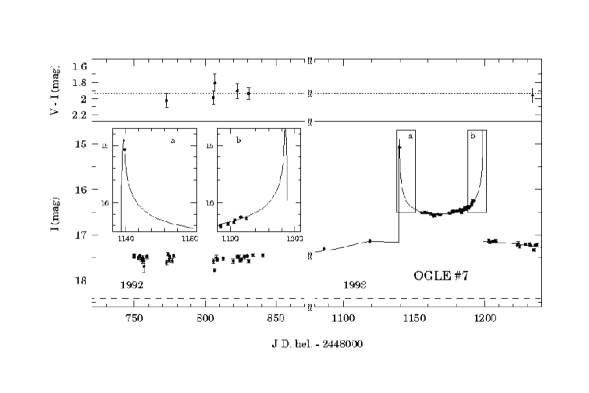
Figure 12: ML event due to a binary lens observed by the OGLE collaboration, reprinted with permission from The Astrophysical Journal.

The first binary lens event detected by OGLE is shown in Fig. 12 (taken from Ref. [173]). It presents two maxima and a characteristic U–shaped plateau between them which is due to the extra pair of images produced when the source crosses the caustic. The best fitting model consists of two nearly equal mass lenses ($q=1.02$), separated by a distance of the order of the total mass Einstein radius ($a/R_{E}=1.14$), with the center of mass passing close to the l.o.s. to the source ($b/R_{E}=0.05$) at an angle $\theta=48^{\circ}.3$. It was a long duration event with $T=80$ d. The estimated contribution by the lensed star to the light–curve at the baseline is $f=56\%$. The MACHO data [153] provides a nice confirmation of the event with a very good coverage of the second caustic crossing which was largely missed by OGLE. Fitting the second caustic crossing points to the magnification near a caustic for a finite size source star with a realistic limb darkening [174], they fixed the time that the diameter of the star took to cross the caustic to be 10 hours, and from this proper motion measurement they estimated the lens relative velocity to be $v^{\perp}=x(48$ km/sec)$R_{s}/R_{\odot}$.

The second event, found by DUO, presents three different peaks with a plateau between the first two [132]. In the best fit model, the source trajectory has two caustic crossing and passes near a cusp, where the third peak arises. The time duration is $T=8.5$ days, suggesting that the total mass is $\sim 10^{-2}M_{\odot}$. The ratio of masses is $q\simeq 0.33$, so that the mass of the lighter lens is close to that of Jupiter. The size of the source is not well constrained in this case, due to poor sampling near the caustic crossing. The estimated fraction of the light contribution at the baseline from the lensed source is $f=70\%$. Further analysis of the data showed some evidence of a shift in the light centroid, as expected when blending with an unlensed source is present. This hypothesis and the estimated location of the unlensed star are confirmed by two good quality images of the object, obtained a posteriori, in which the two stars are resolved.

Another situation in which binarity could play a role is the possibility of ML events in which one member of a binary is lensed by its companion [154, 175]. Gould [175] estimated that the optical depth of these processes is extremely small, $\tau\leq 10^{-11}$, for binaries in which at least one member is an ordinary (non–compact) star.

A further possibility which has been analysed is that planetary systems of Galactic disk stars might be detected by ML of stars in the Galactic bulge [172, 169]. Typical planetary signals produce a deviation from the standard, single lens, light–curve for only a small fraction of the event duration time. The observation of these features would allow one to determine the ratio of the planet and star masses. Gould and Loeb [169] estimated that for about $20\%$ of the lensing events in the bulge due to Solar–type disk stars having Jupiter–like planets, there should be a noticeable signature ($>5$% amplification) of planetary lensing in their light–curves. Due to the short duration of the planetary signal (1 d for a Jupiter mass planet), several observations per day are required in order to pick it up. The GMAN (Global Microlensing Alert Network) [105] and PLANET (Probing Lensing Anomalies Network) collaborations already started the intense scrutiny of alerted events to look for such signals, using telescope networks around the globe.

Hardy and Walker [176] have proposed looking for parallax effects in binary lens events using three 1 m ground based telescopes. The fact that the light–curve is very steep when the limb of the source touches the caustic allows a quite precise determination of the location of the source with respect to the caustic. This would allow one to observe parallax effects by combining observations from distant Earth locations. In this way the angular Einstein ring radius divided by the total lens mass, $\theta_{E}/m_{T}$, can be determined. Since a detailed measurement of the caustic crossing may also allow one to infer the proper motion, these observations could determine the three lens parameters, $m$, $v^{\perp}$ and $D_{ol}$ simultaneously.

Finally, another method for extracting information about the lens parameters for an ordinary ML event, in the case in which both the lens and the source are main–sequence stars, has been proposed by Kamionkowski [177, 178]. If the light from the lens contributes significantly to the observed brightness and it has a different color from the source light, it is expected that for some of the events a shift in the color can be measured. In this case, it would be possible to infer the lens and source colors and luminosities, and hence the lens mass and the distances to the source and the lens if they are main–sequence stars. Using then the event duration one may determine the lens velocity. However, it would be difficult to be sure that the blending in the light is due to light from the lens rather than from another unresolved source. A discussion of the effects of blending in ML searches can be found in Ref. [179].

6 Additional searches

In this Section we discuss the method of searching for ML of unresolved stars which is being applied to ML searches in the Andromeda galaxy. We also discuss the constraints on the number of red and brown dwarfs in the Galaxy, which can be obtained with IR searches and which give important information, complementary to that obtained with ML searches, about the possible Galactic lensing populations.

6.1 Microlensing of unresolved stars

The standard microlensing technique discussed so far consists of monitoring the light flux from a large number of stars, looking for magnifications consistent with the ML event characteritics. This is the method used by the ongoing searches towards the Magellanic Clouds (MACHO and EROS) and the Galactic bulge (OGLE, MACHO and DUO). While this kind of search has led to spectacular results, it has the restriction that it can only be applied to targets where several million stars can be resolved.

A different approach has been proposed by Baillon et al. [180, 181] and by Crotts [182], which consists in the search for ML of unresolved stars. The idea is to study the flux of light received by every CCD pixel in the picture of a galaxy, rather than the flux of the individual stars. This allows one to detect the amplification due to the lensing of one of the many stars present in a crowded field, even if the star is not resolved. The number of stars effectively monitored is greatly enlarged with this method. However, ML events are harder to detect since the light of each star contributes only a small fraction of the light in a pixel. Thus, only lensing of bright stars or very small impact parameter (high amplification) events in the lensing of fainter stars can be detected. It has been proposed that this method, applied to LMC searches, would give an order of magnitude more events than the standard technique [183]. However, the main advantage of the pixel lensing method is that it allows one to look for ML events in more distant galaxies, where the standard lensing technique is not applicable due to the crowding limit. An interesting target for this kind of search is the Andromeda galaxy (M31) [182, 181], which is located at a distance of $\sim 770$ kpc from us. These observations are not only sensitive to ML by compact objects in the Milky Way, but also to those in Andromeda itself. Observations towards M87 in the Virgo cluster may be sensitive to intra–cluster dark matter also [184].

The theory and observational prospects for pixel lensing searches have been studied in Refs. [181, 185, 186, 187, 188]; we present here a brief discussion. The basic idea of the method is that if a star of flux $F_{\star}$ is lensed in a crowded field, by subtracting from the actual images of the field a reference one (obtained by averaging several images taken before or after the event), one should get just a stellar image with flux equal to $(A-1)F_{\star}$ on top of the photon noise. The extent of the star image is fixed by the point spread function (PSF), determined in turn by the actual seeing conditions. If we denote by $\Omega_{PSF}$ the effective solid angle associated with the spread in the star image, and by $\Sigma=\Sigma_{sky}+\Sigma_{gal}$ the background flux per unit solid angle coming from the sky and from the galaxy light in the region where the ML event is taking place, the signal to noise of the ML observation in an exposure time $t_{exp}$ is just

$$\frac{S}{N}=\frac{(A-1)F_{\star}t_{exp}}{\sqrt{\Sigma\Omega_{PSF}t_{exp}}}.$$ (71)

For a required value of $S/N$, there is thus a minimum amplification $A_{min}$, which depends on $F_{\star}$, for the event to be detected.

The strategy adopted, for instance, by the AGAPE group is to study the light–curve of superpixels, i.e. groups of pixels chosen so as to approximately match the PSF of the stellar images, and look for consecutive increments of the signal significantly above the noise to identify a stellar variability. One may also trigger on the signal to noise of the whole event, as advocated in [187, 188].

There are, of course, sources of fluctuations which have to be controlled for a successful observation. These include the limited precision in the telescope pointing (which requires a geometric realignment of the images), the changes in the background sky light and in the transparency of the atmosphere (requiring a photometric realignment of the images) and finally, to eventually convolve the reference image with the actual seeing conditions. Some techniques have been developed to correct for these effects [186, 189], and it is expected that they can be kept smaller than the statistical fluctuations in the number of photons.

As for the standard ML searches, the main background for lensing events of unresolved stars is given by variable stars. The criteria to distinguish them are also the symmetric shape of the light–curve and the non repetition of the ML event. Also the achromaticity signature can be used [186]: even if the lensing of a star will cause a color variation in the pixels involved, the ratio of the increment in the flux from the reference flux in two different colors

$$\frac{(F-\langle F_{ref}\rangle)_{red}}{(F-\langle F_{ref}\rangle)_{blue}}=\frac{(F_{\star})_{red}}{(F_{\star})_{blue}}$$ (72)

is constant in time during an ML event.

Another point which has to be taken into account in ML searches in distant galaxies is that the effect of the finite size of the source gives rise to a maximum amplification, given by Eq. (61), as discussed in the previous section. Thus, for sources of a given radius $R_{s}$, there is a minimum lens mass giving rise to an observable event

$$m_{min}=0.7\times 10^{-7}M_{\odot}(1+A^{2}_{min})\left(\frac{R_{s}}{R_{\odot}}\right)^{2}\left(\frac{1\ {\rm kpc}}{D_{ls}}\right),$$ (73)

where $A_{min}$ is the threshold amplification associated to a given $S/N$ requirement. This has the effect of reducing the number of detectable lensing events of red giant sources and the efficiency for lensing by very light objects in M31 [181].

Using Monte Carlo simulations and semi–analytic computations, Baillon et al. [181] estimated that in searches towards M31 the best sensitivity is achieved for lens masses in the range $10^{-3}$–$10^{-5}M_{\odot}$, that most of the detectable events correspond to mild amplifications of bright stars rather than high amplifications of faint ones, and that feasible observation programs would lead to a few tens of events per year for brown dwarf masses in the range $10^{-5}$ to $10^{-1}M_{\odot}$ making up the halos of the Milky Way and M31. Similar conclusions were reached in Ref. [185].

Two groups have already started observational programs towards M31 with the aim of proving the feasibility of the pixel lensing technique and have already been able to identify variability of unresolved stars. AGAPE (Andromeda Galaxy Pixel Experiment) is a French collaboration that has taken data using a 2 m telescope with a CCD camera at the Pic du Midi observatory during observing periods in 1994 and 1995 [186]. The Columbia–VATT collaboration is an experiment led by Crotts using mainly the Vatican Telescope in Arizona [189].

6.2 Microlensing towards Andromeda

The Andromeda galaxy provides a very interesting target for microlensing. It is the closest large galaxy, and as it is located forming an angle of $119^{\circ}$ with respect to the Galactic center, it provides a possibility for testing the dark constituency of the Galaxy in a direction complementary to the Galactic bulge and LMC targets. Moreover, the dark constituency of M31 itself can be probed, and the fact that we see the disk of M31 with a high inclination ($i\simeq 75^{\circ}$ respect to the face on position) gives rise, for lenses in M31, to a much larger optical depth for ML of sources in the far side of the disk than for those in the near side [182, 181, 74]. This effect arises because the l.o.s. to the far side of M31 goes through much of the inner and denser part of the M31 halo and spheroid, and provides an interesting signature of ML.

The probability of observing an ML event in a crowded field can be estimated as follows. First, we estimate the probability that a star of a given luminosity $L$ in the field gives rise to an observable event, and then sum over all the stars

$$\tau_{pixel}=\sum_{stars}\tau(L).$$ (74)

Here the sum over the stars is performed by integrating over the luminosity function (normalized to the surface brightness of the galaxy). This was performed for the case of M31 in Refs. [181, 185] using the available measurements for red giants and a matching for fainter stars with the luminosity function in the solar neighbourhood conveniently normalised. To observe an ML event of a star of luminosity $L$, the mean amplification during the exposure has to be larger than a threshold amplification $A_{min}$ given by the minimum $S/N$ required through Eq. (71), or equivalently the lensing object has to be at a distance from the l.o.s. smaller than the corresponding $u_{max}(L)$ obtained from Eq. (16). Thus, the probability that a star of luminosity $L$ be lensed to observable levels is just the number of lenses inside a tube of radius $u_{max}(L)R_{E}$ around the l.o.s., that is $u^{2}_{max}(L)\tau_{\star}$, where $\tau_{\star}$ is the optical depth for the standard ML of a star as given by Eq. (19).

Thus, the optical depth for unresolved stars can be estimated as

$$\tau_{pixel}=\tau_{\star}\sum_{stars}u^{2}_{max}(L).$$ (75)

If the lenses belong to M31, the dependence of $\tau_{\star}$ on the observation position in M31 can be readily obtained from Eq. (19), using for $\rho(r)$ the density of M31 lensing objects, with $r$ being the distance of the lens to the M31 center,

$$r=\sqrt{(D_{os}-D_{ol}-d\cos\Phi\tan i)^{2}+d^{2}},$$ (76)

where $i\simeq 75^{\circ}$ is the inclination angle of the M31 disk, $d$ is the distance between the l.o.s. to the source and the M31 center, and $\Phi$ its angle to the far minor axis. Crotts [182] obtained the resulting $\tau_{\star}$ for a spherically symmetric halo. The non-spherical axisymmetric case has been analysed in Ref. [190]. The contribution from a heavy spheroid has been computed in Ref. [74], while that of a disk population has been obtained in Ref. [191].

Figure 13: Optical depth for ML by halo and heavy spheroid populations of Andromeda (M31) and the Milky Way (MW), as a function of the impact parameter between the l.o.s. to stars in the minor axis of M31 and the M31 center.

Figure 13 shows the optical depth dependence on $d$ for stars along the minor axis and lenses with the Milky Way and Andromeda halo and heavy spheroid density distributions (from Ref. [74]). If observations at different distances are performed, they would clearly yield valuable information about the distribution of the lenses.

6.3 Infrared searches for low mass dwarfs

There are other observations which can be helpful for identifying the lensing population. If the dark objects responsible for ML are in the form of low mass red dwarfs ($m\sim 0.1$–$0.2M_{\odot}$), which are very faint and emit mostly in the IR, or of brown dwarfs, i.e. stars not massive enough to burn hydrogen but which emit anyway due to their gravitational contraction and degenerate cooling [192], they could be detected via their infrared emission [193, 194, 195, 196, 197, 198, 199, 200]. The most promising brown dwarf signal comes from individual stars in the solar vicinity, while the collective emission from Galactic or extra–Galactic brown dwarf distributions is generally less important.

Assuming that brown dwarfs emit black body radiation, the peak flux of the nearest brown dwarf of a population with local density $\rho_{0}$ is [197]

$$F_{max}=0.018\left(\frac{\rho_{0}}{0.01M_{\odot}{\rm pc}^{-3}}\right)^{2/3}\left(\frac{m}{0.01M_{\odot}}\right)^{1.04}\left(\frac{\tau}{10^{10}{\rm yr}}\right)^{-0.94}\left(\frac{\kappa}{10^{-2}{\rm cm}^{2}{\rm g}^{-1}}\right)^{0.225}{\rm Jy}.$$ (77)

Here $m$, $\tau$, and $\kappa$ are respectively the mass, age and opacity of the nearest brown dwarf (${\rm Jansky}=10^{-23}$erg cm^-2s^-1Hz^-1). The flux peaks at the wavelength

$$\lambda_{max}=23\left(\frac{m}{0.01M_{\odot}}\right)^{-0.79}\left(\frac{\tau}{10^{10}{\rm yr}}\right)^{0.31}\left(\frac{\kappa}{10^{-2}{\rm cm}^{2}{\rm g}^{-1}}\right)^{-0.075}\mu{\rm m}.$$ (78)

For a disk population of brown dwarfs, it is appropriate to take $\tau\simeq 5\times 10^{9}$ yr and $\kappa\simeq 1$ cm² g^-1. Therefore, the present constraint on infrared emission from the $IRAS$ survey [202], $F_{max}<0.2$ Jy for $\lambda=12\mu$m, already sets a significant bound on the number of brown dwarfs in the thin disk.

On the other hand, for the heavy spheroid and halo populations (for which it is reasonable to take $\tau=10^{10}$ yr and $\kappa=10^{-2}$ cm² g^-1, appropriate for older stars) the maximum fluxes are $\sim 0.03(m/0.05M_{\odot})$ Jy and $0.1(m/0.05M_{\odot})$ Jy respectively, therefore below the $IRAS$ survey sensitivity. Nevertheless, the situation will be improved in the near future by observations with the recently launched satellite $ISO$, and later with $SIRTF$.

The content of low mass red dwarfs in the Galactic halo is also constrained by near IR searches [198, 199, 200]. These limits again come from the effects of individual stars, as the diffuse emission suffers from large uncertainties from the background. Boughn and Uson [200] found that no more than 3$\%$ of a standard halo ($\rho_{0}^{H}=0.01M_{\odot}$ pc^-3, $a=4$ kpc) can be in the form of red dwarfs of $m>0.1M_{\odot}$, using the result of a deep IR survey by Cowie et al. [203]. Pushing the local halo density to the minimum limit by considering a ‘maximum disk’ model relaxes the limit to $6\%$. Tight bounds on the halo density in red dwarfs were also obtained by Hu et al. [199] using data from four high latitude sky strips in the near infrared. Another study by Bahcall et al. [198] of two long exposures of a high latitude field taken with the Wide Field camera on the Hubble Space Telescope, also constrains the local density of red dwarfs. They set a limit to the red dwarf contribution (in stars with $V-I>3$ and $M_{I}>15$) to the local column density of the thin disk of $\Sigma<8M_{\odot}$ pc^-2, and of $\Sigma<10M_{\odot}$ pc^-2 for stars in the thick disk. The contribution of main–sequence stars with $M_{I}>10$ to the dark halo is constrained to be less than 6%. A reanalysis of this same data by Graff and Freese [204], using new stellar models and parallax measurements of low mass, low metallicity stars, tightens this last bound to be less than 1% of the halo density.

This means that if a significant fraction of the Galactic halo consists of a population of brown and red dwarfs, then their mass function has to cut off very sharply above $0.1M_{\odot}$.

7 Conclusions

The idea of using ML to study the dark constituents of our Galaxy has proved to be extremely useful. In the last few years, several experiments started searches for ML and many surprises have resulted.

The observations in the direction of the LMC returned rates which are significantly smaller than those expected from a standard halo composed of objects with masses in the range $10^{-7}$–$10^{-1}M_{\odot}$, but anyway larger than those expected from the faint stars present in the known stellar populations, so that something new has certainly been found. If the compact objects belong to the halo, these results could imply that the halo has a large fraction of heavy objects ($m>0.1M_{\odot}$), or a lot of gas, or is a mixture with non–baryonic dark matter, or alternatively that it deviates significantly from the standard halo models due, for instance, to the disk being close to maximal and the rotation curve actually falling with distance. Another plausible explanation is that a large number of brown dwarfs and/or stellar remnants is present either in the Galactic spheroid or in a thick disk, with the halo being allowed to be completely non–baryonic. Increased statistics will clearly allow these facts to be put on a more solid basis and to discriminate between the different proposed solutions. Continuing the observations will also allow one to gain sensitivity to longer event durations, i.e. to heavier lens masses.

Observations towards the bulge returned on the contrary more events than were initially expected, implying that probably the bar in the inner Galaxy was rediscovered using ML. Continued searches will allow one to further constrain the geometry and mass of this Galactic component. The rates observed may also be indicative of large amounts of material in the disk, and this could also hint towards a smaller contribution of the halo to the rotation curve, so that bulge results may also be relevant for LMC searches. The large number of events observed has allowed identification of some particularly interesting cases of ML, such as events due to binary lenses and the observation of parallax due to the Earth’s motion. More events of these types, as well as proper motion measurements in the lensing of giant stars, will allow better identification of the lensing agents. Also the mapping of the rates and event durations across the bulge are crucial for isolating the different contributions from disk and bulge lens and source populations.

Hence, microlensing has opened a new window for Galactic astronomy, allowing one to ‘see’ dark objects which are otherwise unobservable. The first results already had an important impact on our understanding of Galactic structure and of the composition of the dark halo, which still remains one of the fundamental open problems in physics. This field is rapidly moving, with new experiments joining the searches, so that one can expect that a deeper, and better established, knowledge of these fundamental issues, and possibly some new surprises, will be obtained in the near future.

Note added

Just after completing this review, the first new ‘surprising’ ML result was announced by the MACHO collaboration. They presented their preliminary results from the analysis of the second year of LMC data as well as a reanalysis of the first year data, exploiting the experience gained with the large number of ML events observed towards the bulge. They realized that many of the bulge events would not have been identified with the cuts employed in the initial analysis of the first year of LMC data, and hence used a different search strategy in the new analysis. The results were:

i) Of the three events found initially [103], only one remained as a ‘true’ ML event, the one shown in Figure 8. Of the other two, which were low signal events, one had other bumps in the light–curve during the second year, being shown then to be just a variable, and the other one did not pass the new cuts. However, the star sample was enlarged by 15% in the reanalysis of the first year data, and with the new cuts two new events appeared during this period.

ii) Regarding the second year, five candidate events were found, one of which is slightly asymmetric, and hence not completely reliable. Another of these events is due to a binary lens, and it was possible to measure the proper motion during one of the caustic crossings. The small value of this quantity ($\mu\simeq 2$ km/s/kpc) suggests that the lens belongs to the LMC. On the other hand, for the accumulated statistics, about one event was expected due to LMC stars acting as lenses, and the binary event appeared just in a star in the LMC bar, while most of the remaining events are in stars outside the bar, and hence are less likely to be due to LMC lenses.

iii) Another important fact is that the durations of all the new events are longer (23 d to 72 d) than those found initially in the first year analysis, implying that the inferred lens masses ($m\simeq 0.1$–$1M_{\odot}$) are larger than initially suggested.

iv) A preliminary estimate of the optical depth from the eight events is $\tau\simeq 2.5^{+1.2}_{-0.7}\times 10^{-7}$, while removing the asymmetric event and the binary lens one (since the lens belongs to the LMC), leads to an estimated $\tau\simeq 1.7^{+0.9}_{-0.5}\times 10^{-7}$ for the optical depth due to the lenses which could be Galactic.

v) MACHO did a ‘spike’ search, looking for short duration events ($T<1$ d) leading to a couple of high amplification points in the light–curve during one night and in the two colors. No event was found, resulting in significant constraints for the low mass range ($m\sim 10^{-7}$–$10^{-3}M_{\odot}$).

References

- [1] A. S. Eddington, Observatory 42, 119 (1919).
- [2] A. S. Eddington, Space, Time and Gravitation (Cambridge University Press, Cambridge, 1920).
- [3] O. Chwolson, Astr. Nachrichten 221, 329 (1924).
- [4] A. Einstein, Science 84, 506 (1936).
- [5] F. Zwicky, Phys. Rev. 51, 290 (1937).
- [6] F. Zwicky, Phys. Rev. 51, 679 (1937).
- [7] D. Walsh, R. F. Carswell, and R. J. Weymann, Nature 279, 381 (1979).
- [8] P. Schneider, J. Ehlers, and E. E. Falco, Gravitational Lenses (Springer-Verlag, Berlin, Heildelberg, New York, 1992).
- [9] R. D. Blandford and R. Narayan, ARA&A 30, 311 (1992).
- [10] S. Refsdal and J. Surdej, Rep. Prog. Phys. 57, 117 (1994).
- [11] J. A. Tyson and P. Fischer, ApJ 446, L55 (1995).
- [12] S. Liebes, Phys. Rev. 133B, 835 (1964).
- [13] S. Refsdal, MNRAS 128, 295 (1964).
- [14] K. Chang and S. Refsdal, Nature 282, 561 (1979).
- [15] W. H. Press and J. E. Gunn, ApJ 185, 397 (1973).
- [16] J. R. Gott, ApJ 243, 140 (1981).
- [17] B. Paczyński, ApJ 304, 1 (1986).
- [18] B. Paczyński, ApJ 371, L63 (1991).
- [19] K. Griest et al., ApJ 372, L79 (1991).
- [20] C. Alcock et al., Nature 365, 621 (1993).
- [21] E. Aubourg et al., Nature 365, 623 (1993).
- [22] A. Udalski et al., Acta Astron. 43, 289 (1993).
- [23] M. Fich and S. Tremaine, ARA&A 29, 409 (1991).
- [24] K. C. Freeman, ARA&A 25, 603 (1987).
- [25] J. N. Bahcall, ARA&A 24, 577 (1986).
- [26] K. M. Ashman, Proc. Astron. Soc. Pac. 104, 1109 (1992).
- [27] F. Zwicky, Helvetica Physica Acta 11, 110 (1933).
- [28] S. D. M. White, J. F. Navarro, A. E. Evrard, and C. S. Frenk, Nature 366, 429 (1993).
- [29] R. Sancisi and T. S. van Albada, in Dark Matter in the Universe, edited by J. Kormendy and G. R. Knapp (Reidel, Dordrecht, 1987), p. 67.
- [30] M. Persic and P. Salucci, ApJ Suppl. 99, 501 (1995).
- [31] D. Zaritsky and S. D. White, ApJ 435, 599 (1994).
- [32] J. P. Ostriker, P. J. E. Peebles, and A. Yahil, ApJ 193, L1 (1974).
- [33] J. A. Caldwell and J. P. Ostriker, ApJ 251, 61 (1981).
- [34] E. Gates, G. Gyuk, and M. Turner, ApJ 449, L123 (1995).
- [35] J. A. Sellwood and R. H. Sanders, MNRAS 233, 611 (1988).
- [36] H. W. Rix, in Unsolved problems of the Milky Way, IAU Symp. 169, edited by L. Blitz (Reidel, Dordrecht, 1995).
- [37] S. R. Kulkarni, L. Blitz, and C. Heiles, ApJ 259, L63 (1982).
- [38] M. R. Merrifield, AJ 103, 1552 (1992).
- [39] N. W. Evans, MNRAS 267, 333 (1994).
- [40] K. Kuijken and J. Dubinsky, astro–ph/9502069.
- [41] C. J. Copi, D. N. Schramm, and M. S. Turner, Science 267, 192 (1995).
- [42] B. Pagel, Baryonic Dark Matter (Kluwer, Dordrecht, 1990), p. 237.
- [43] M. Persic and P. Salucci, MNRAS 258, 14P (1992).
- [44] E. Bertschinger and A. Dekel, ApJ 336, L5 (1989).
- [45] B. Carr, ARA&A 32, 531 (1994).
- [46] C. Low and D. Lynden-Bell, MNRAS 176, 367 (1976).
- [47] F. Palla, E. E. Salpeter, and S. W. Stahler, ApJ 271, 632 (1983).
- [48] A. De Rújula, P. Jetzer, and E. Massó, A&A 254, 99 (1992).
- [49] D. Pfenniger, F. Combes, and L. Martinet, A&A 285, 79 (1994).
- [50] F. De Paolis, G. Ingrosso, P. Jetzer, and M. Roncadelli, Phys. Rev. Lett. 74, 14 (1995).
- [51] O. Gerhard and J. Silk, astro–ph/9509149.
- [52] S. Charlot and J. Silk, ApJ 445, 124 (1995).
- [53] S. M. Kent, T. M. Dame, and G. Fazio, ApJ 378, 131 (1991).
- [54] J. N. Bahcall and S. Casertano, ApJ 308, 347 (1986).
- [55] B. Paczyński et al., AJ 107, 2060 (1994).
- [56] J. R. Lewis and K. C. Freeman, AJ 97, 139 (1989).
- [57] G. Gilmore and N. Reid, MNRAS 202, 1025 (1983).
- [58] J. N. Bahcall, ApJ 276, 169 (1984).
- [59] A. Gould, J. N. Bahcall, and C. Flynn, ApJ 465, 000 (1996).
- [60] K. Kuijken and G. Gilmore, ApJ 367, L9 (1991).
- [61] A. Gould, MNRAS 244, 25 (1990).
- [62] J. N. Bahcall, C. Flynn, and A. Gould, ApJ 389, 234 (1992).
- [63] J. M. Scalo, Fundamentals of Cosmic Physics 11, 1 (1986).
- [64] C. G. Tinney, ApJ 414, 279 (1993).
- [65] A. Gould, ApJ 421, L71 (1994).
- [66] A. Gould, J. Miralda-Escudé, and J. N. Bahcall, ApJ 423, L105 (1994).
- [67] M. Rich, ApJ 362, 604 (1990).
- [68] J. Binney and A. May, MNRAS 218, 743 (1986).
- [69] L. Blitz and D. N. Spergel, ApJ 370, 205 (1991).
- [70] J. N. Bahcall, M. Schmidt, and R. M. Soneira, ApJ 265, 730 (1983).
- [71] J. P. Ostriker and J. A. R. Caldwell, in Dynamics and Structure of the Milky Way, edited by W. L. H. Shuter (Reidel, Dordtrecht, 1982).
- [72] K. Rohlfs and J. Kreitschmann, A&A 201, 51 (1988).
- [73] H. B. Richer and G. G. Fahlman, Nature 358, 383 (1992).
- [74] G. F. Giudice, S. Mollerach, and E. Roulet, Phys. Rev. D50, 2406 (1994).
- [75] V. M. Blanco and D. M. Terndrup, AJ 98, 843 (1989).
- [76] A. McWilliam and R. M. Rich, ApJ Suppl. Series 91, 749 (1994).
- [77] D. Minniti, ApJ 459, 175 (1996).
- [78] R. M. Rich, in The Center, Bulge, and Disk of the Milky Way, edited by L. Blitz (Kluwer, Dordrecht, 1992), p. 47.
- [79] R. F. G. Wyse and G. Gilmore, AJ 104, 144 (1992).
- [80] L. Blitz and D. N. Spergel, ApJ 379, 631 (1991).
- [81] S. M. Kent, ApJ 387, 181 (1992).
- [82] E. Dwek et al., ApJ 445, 716 (1995).
- [83] D. N. Spergel, in The Center, Bulge, and Disk of the Milky Way, edited by L. Blitz (Kluwer, Dordrecht, 1992), p. 77.
- [84] J. Binney et al., MNRAS 252, 210 (1991).
- [85] R. D. Blum, ApJ 444, L89 (1995).
- [86] C. Han and A. Gould, astro–ph/9504078.
- [87] E. Gates, G. Gyuk, and M. Turner, astro–ph/9508071.
- [88] C. Han and A. Gould, ApJ 447, 53 (1995).
- [89] H. Zhao, D. N. Spergel, and R. M. Rich, ApJ 440, L13 (1995).
- [90] H. Zhao, R. M. Rich, and D. N. Spergel, astro–ph/9512065.
- [91] R. J. Nemiroff, A&A 247, 73 (1991).
- [92] K. Griest, ApJ 366, 412 (1991).
- [93] A. De Rújula, P. Jetzer, and E. Massó, MNRAS 250, 348 (1991).
- [94] A. De Rújula, G. F. Giudice, S. Mollerach, and E. Roulet, MNRAS 275, 545 (1995).
- [95] M. Vietri and J. P. Ostriker, ApJ 267, 488 (1983).
- [96] M. Kiraga and B. Paczyński, ApJ 430, L101 (1994).
- [97] H. B. Richer et al., ApJ 381, 147 (1991).
- [98] P. Jetzer and E. Massó, Phys. Lett. B323, 347 (1994).
- [99] C. Alcock et al., AJ 109, 1653 (1995).
- [100] P. Grison et al., A&A Suppl. Ser. 109, 447 (1995).
- [101] J. P. Beaulieu et al., A&A 303, 137 (1995).
- [102] A. Udalski et al., Acta Astron. 45, 1 (1994).
- [103] C. Alcock et al., astro–ph/9506113.
- [104] S. Benetti, L. Pasquini, and R. M. West, A&A 294, L37 (1995).
- [105] M. R. Pratt et al., in IAU Symposium 173, Astrophysical Applications of Gravitational Lensing, edited by C. S. Kochanek and J. N. Hewitt (Kluwer Academic, Dordrecht, 1995).
- [106] A. Udalski et al., Acta Astron. 44, 227 (1994).
- [107] B. Paczyński, Acta Astr. 44, 235 (1994).
- [108] R. Taillet, P. Longaretti, and P. Salati, Astroparticle Phys. 4, 87 (1995).
- [109] E. Aubourg et al., A&A 301, 1 (1995).
- [110] R. Ansari et al., astro–ph/9511073.
- [111] R. Ansari et al., A&A 299, L21 (1995).
- [112] C. Han and A. Gould, ApJ 449, 521 (1995).
- [113] C. Alcock et al., ApJ 449, 28 (1995).
- [114] X. P. Wu, ApJ 435, 66 (1994).
- [115] C. Alcock et al., Phys. Rev. Lett. 74, 2867 (1995).
- [116] E. Gates and M. Turner, Phys. Rev. Lett. 72, 2520 (1994).
- [117] E. Gates, G. Gyuk, and M. Turner, Phys. Rev. Lett. 74, 3724 (1995).
- [118] E. J. Kerins, MNRAS 276, 785 (1995).
- [119] R. N. Henriksen and L. Widrow, ApJ 441, 70 (1995).
- [120] N. W. Evans and J. Jijina, MNRAS 267, L21 (1994).
- [121] Y. Kan-ya, R. Nishi, and T. Nakamura, astro–ph/9505130.
- [122] F. de Paolis, G. Ingrosso, and P. Jetzer, astro–ph/9510099.
- [123] N. W. Evans, astro–ph/9510016.
- [124] P. D. Sackett and A. Gould, ApJ 419, 648 (1993).
- [125] J. Frieman and R. Scoccimaro, ApJ 431, L23 (1994).
- [126] G. P. Holder and L. M. Widrow, astro–ph/9510023.
- [127] B. E. Westerlund, in The Magellanic Clouds, edited by R. Haynes and D. Milne (Kluwer Academic, Dordrecht, 1991).
- [128] R. A. Schommer, E. W. Olszewski, N. B. Suntzeff, and H. C. Harris, AJ 103, 447 (1992).
- [129] A. Gould, ApJ 404, 451 (1993).
- [130] K. C. Sahu, Nature 370, 275 (1994).
- [131] A. Gould, ApJ 441, 77 (1995).
- [132] C. Alard, S. Mao, and J. Guibert, A&A 300, L17 (1995).
- [133] A. Udalski et al., Acta Astron. 44, 165 (1994).
- [134] C. Alcock et al., ApJ 445, 133 (1995).
- [135] C. Alcock et al., astro–ph/9512146.
- [136] E. Roulet, S. Mollerach, and G. Giudice, in Neutrino 94, edited by M. B. Ceolin (INFN, Padova, 1994).
- [137] B. Paczyński et al., ApJ 435, L113 (1994).
- [138] N. W. Evans, ApJ 437, L31 (1994).
- [139] K. Z. Stanek et al., ApJ 429, L73 (1994).
- [140] K. Z. Stanek, ApJ 441, L29 (1995).
- [141] A. Gould, ApJ 446, L71 (1995).
- [142] S. Mollerach and E. Roulet, ApJ 458, L9 (1996).
- [143] D. M. Terndrup, AJ 96, 884 (1988).
- [144] S. Refsdal, MNRAS 134, 315 (1966).
- [145] B. Grieger, R. Kayser, and S. Refsdal, Nature 324, 126 (1986).
- [146] R. Kayser, S. Refsdal, and R. Stabell, A&A 166, 36 (1986).
- [147] A. Gould, ApJ 392, 442 (1992).
- [148] A. Gould, ApJ 421, L75 (1994).
- [149] A. Gould, ApJ 441, L21 (1995).
- [150] T. Boutreux and A. Gould, ApJ 462, 000 (1996).
- [151] B. S. Gaudi and A. Gould, astro–ph/9601030.
- [152] C. Alcock et al., ApJ 454, L125 (1995).
- [153] D. P. Bennett et al., AIP Conference Proceedings 336: Dark Matter, edited by S. S. Holt and C. L. Bennett (1995).
- [154] A. Maeder, A&A 26, 215 (1973).
- [155] H. J. Witt and S. Mao, ApJ 430, 505 (1994).
- [156] R. J. Nemiroff and W. A. Wickramasinghe, ApJ 424, L21 (1994).
- [157] M. R. Pratt et al., BAAS 27, 1351 (1995).
- [158] A. Gould, ApJ 447, 491 (1995).
- [159] H. J. Witt, ApJ 449, 42 (1995).
- [160] A. Gould and D. L. Welch, ApJ 464, 000 (1996).
- [161] A. Loeb and D. Sasselov, ApJ 449, L33 (1995).
- [162] J. F. L. Simmons, J. P. Willis, and A. M. Newsam, A&A 293, L46 (1995).
- [163] D. Maoz and A. Gould, ApJ 425, L67 (1994).
- [164] M. A. Walker, ApJ 453, 37 (1995).
- [165] H. A. Abt, ARA&A 21, 243 (1983).
- [166] K. Griest and W. Hu, ApJ 397, 362 (1992), erratum: ApJ 407, 440 (1993).
- [167] P. Schneider and A. Weiss, A&A 164, 237 (1986).
- [168] H. J. Witt, A&A 236, 311 (1990).
- [169] A. Gould and A. Loeb, ApJ 396, 104 (1992).
- [170] H. J. Witt and S. Mao, ApJ 447, L105 (1995).
- [171] S. Mao and R. Di Stefano, ApJ 440, 22 (1995).
- [172] S. Mao and B. Paczyński, ApJ 374, L37 (1991).
- [173] A. Udalski et al., ApJ 436, L103 (1994).
- [174] P. Schneider and R. V. Wagoner, ApJ 314, 154 (1987).
- [175] A. Gould, ApJ 446, 541 (1995).
- [176] S. J. Hardy and M. A. Walker, MNRAS 276, L79 (1995).
- [177] M. Kamionkowski, ApJ 442, L9 (1995).
- [178] A. Buchalter, M. Kamionkowski, and R. M. Rich, astro–ph/9511034.
- [179] R. D. Stefano and A. A. Esin, ApJ 448, L1 (1995).
- [180] P. Baillon, A. Bouquet, J. Kaplan, and Y. Giraud-Héraud, in First Palaiseau Symposium on Atmospheric Cerenkov Techniques, edited by P. Fleury and G. Vacanti (Edition Frontières, France, 1992), p. 151.
- [181] P. Baillon et al., A&A 277, 1 (1993).
- [182] A. P. S. Crotts, ApJ 399, L43 (1992).
- [183] A. Bouquet et al., in The Dark Side of the Universe, edited by R. Bernabei and C. Tao (World Scientific, Singapore, 1993).
- [184] A. Gould, ApJ 455, 44 (1995).
- [185] W. N. Colley, AJ 109, 440 (1995).
- [186] R. Ansari et al., Texas Symposium on Relativistics Astrophysics, in press, astro–ph/9502102.
- [187] A. Gould, astro–ph/9509009.
- [188] C. Han, astro–ph/9510161.
- [189] A. Tomaney and A. Crotts, 1996, in preparation.
- [190] P. Jetzer, A&A 286, 426 (1994).
- [191] A. Gould, ApJ 435, 573 (1994).
- [192] J. I. Lunine, W. B. Hubbard, and M. S. Marley, ApJ 310, 238 (1986).
- [193] C. A. Beichman et al., AJ 99, 1569 (1990).
- [194] F. C. Adams and T. P. Walker, ApJ 359, 57 (1990).
- [195] R. A. Daly and G. C. McLaughlin, ApJ 390, 423 (1993).
- [196] L. A. Nelson, S. A. Rappaport, and P. C. Joss, ApJ 404, 723 (1993).
- [197] E. J. Kerins and B. J. Carr, MNRAS 266, 775 (1994).
- [198] J. N. Bahcall, C. Flynn, A. Gould, and S. Kirhakos, ApJ 435, L51 (1994).
- [199] E. M. Hu, J. S. Huang, G. Gilmore, and L. L. Cowie, Nature 371, 493 (1994).
- [200] S. P. Boughn and J. M. Uson, Phys. Rev. Lett. 74, 216 (1995).
- [201] V. Kashyap, R. Rosner, D. Schramm, and J. Truran, ApJ 431, L87 (1994).
- [202] M. Moshir et al., Explanatory Supplement to the Faint Source Survey, Version 2, Passadena:JPL, 1992.
- [203] L. Cowie et al., ApJ 360, L1 (1990).
- [204] D. S. Graff and K. Freese, astro–ph/9507097.