A Parallel Tree Code

John Dubinski

Abstract

We describe a new implementation of a parallel N-body tree code. The code is load-balanced using the method of orthogonal recursive bisection to subdivide the N-body system into independent rectangular volumes each of which is mapped to a processor on a parallel computer. On the Cray T3D, the load balance in the range of 70-90% depending on the problem size and number of processors. The code can handle simulations with $>$ 10 million particles roughly a factor of 10 greater than allowed on vectorized tree codes.

Board of Studies in Astronomy and AstrophysicsUniversity of California, Santa Cruz, CA 95064dubinski@ucolick.org

Subject headings: methods: numerical – galaxies: formation – galaxies: kinematics and dynamics – cosmology: theory

1 Introduction

During the past decade, $N$ -body tree codes have been applied successfully to various problems in galaxy dynamics, galaxy formation and cosmological structure formation (Barnes & Hut 1986; Hernquist 1987; Dubinski 1988). Computing time only scales as $N\log N$ so they provide a relatively fast way to solve the general collisionless N-body problem. For the most part, the favored tree code in studies has been the Barnes-Hut (BH) code (1986) mainly because it was widely distributed by its authors but also because it has been easy to implement. Different tree-based algorithms have also been used successfully for various problems (Appel 1985; Jernigan & Porter 1989; 1993; Benz, Bowers, Cameron & Press 1990; Steinmetz & Muller 1993). Tree codes have also been linked up with smoothed particle hydrodynamics (SPH) (Hernquist & Katz 1989; Benz et al 1990; Steinmetz & Muller 1993). Tree code simulations running on the latest workstations and vector supercomputers are generally restricted to $N<10^{6}$ because of memory and time limitations. Cosmological and hydrodynamical simulations require ever greater dynamic range, so there is a strong desire to increase these limits.

During the past few years, there has been a paradigm shift in supercomputing with the movement from vector machines to the new massively parallel machines. Parallel supercomputers are collections of hundreds to thousands of independent smaller commodity processors interconnected with an internal high speed communication network. The NSF supercomputing centers support several machines: the Connection Machine 5, (CM-5), the Intel Paragon, the IBM SP/2, and the Cray T3D. Each processor operates independently but communication software allows messages containing data to be exchanged rapidly with other processors. In principle, a problem can be partitioned among the $N$ processors and a maximum $N$ -fold increase in computational speed can be realized. In practice, the speed up is smaller because of the extra time needed for exchanging data in message-passing algorithms.

Parallel machines offer a new route to very fast computation if algorithms can be redesigned to conform to the message-passing paradigm and communication can be minimized. The new algorithms are often very different than their sequential counterparts and require a considerable effort to redesign. The key to a successful algorithm is good load balance: both data and computational work must be distributed evenly among the processors. A common way of achieving load balance on parallel machines is through domain decomposition (Fox, Williams & Messina 1994). The physical domain of the problem is partitioned into smaller subdomains and the physical quantities of these subdomains: either values of density, pressure and temperature at grid elements in an Eulerian fluid code or collections of particles and their attributes in an N-body code are assigned to each processor. The trick in designing a parallel algorithm is finding a way of partitioning the domain so that data and work are evenly distributed and communication is minimized.

There have been many efforts to parallelize the BH tree code. Hillis and Barnes (1987) and Makino and Hut (1989) ported the code to the Connection Machine-2 but at the time there was little gain over the existing vector machines. Salmon (1990) introduced a new parallel tree algorithm using a domain decomposition based on the orthogonal recursive bisection of the N-body volume into rectangular subvolumes for purposes of load balance. The code has been applied to dark halo formation with initial density fluctuations based on different power spectra (Warren et al. 1992; Warren 1994; Zurek et al. 1994). Warren & Salmon (1993) have also recently designed a new algorithm which uses a load-balancing scheme based on a parallel hashed oct-tree (also Warren 1994). Dikaiakos and Stadel (1995) also have developed another variant of Salmon’s algorithm in their parallel tree code PKDGRAV. Parallel N-body tree codes have also been discussed as a pure computer science problem (Bhatt et al. 1992; Pal Singh 1993; Pal Singh et al. 1995).

In this paper, we present a new version of Salmon’s (1990) parallel tree algorithm. In §2, we describe the BH tree code as implemented at the node level in the parallel code. In §3, we describe a new portable implementation of Salmon’s parallel algorithm using the Message Passing Interface (MPI) package to handle processor communication. In §4, we examine the code’s performance on the Cray T3D, checking the accuracy, speed, and load balance. The term “node” is often used to refer to a single processor on a parallel computer but it is also used to refer to a data structure in a tree. To avoid confusion, I will only use the term “node” in reference to tree structures and “processor” for a computational “node”.

2 Tree Codes

The N-body problem involves advancing the trajectories of $N$ particles according to their time evolving mutual gravitational field. In the simplest algorithm, the force on each particle is determined by direct summation of the contributions from all of the N-1 neighbours. In a discrete integration, the forces at each timestep are then used to advance the particles along their trajectories according to a numerical integration scheme such as the leapfrog method. Computational costs of direct summation scale as $O(N^{2})$ making this algorithm expensive. In collisionless systems like galaxies, however, one can tolerate small errors in the force for improved performance by using techniques which approximate the gravitational field. Tree codes are one class of methods which accomplish this and have the advantage of scaling only as $O(N\log N)$ in computational cost (Appel 1985; Barnes & Hut 1986; Jernigan & Porter 1989).

The essence of a tree code is the recognition that the gravitational potential of a distant group of particles can be well-approximated by a low-order multipole expansion. A set of particles can be arranged in a hierarchical system of groups in the form of a tree structure. The entire set can be subdivided into several groups and each of these groups can be broken down in succession in the hierarchy until the groups contain at most 1 particle. There are many different methods for grouping particles hierarchically in this way (Appel 1985; Jernigan & Porter 1989; Barnes & Hut 1986). The evaluation of the potential at a point reduces to a descent through the tree. One sets a minimum distance a point can be from a group to use a multipole expansion. If the point is sufficiently distant from a group, the multipole expansion is used to find the potential from that group, while if the point is too close to the group, each of its child subgroups are examined. The procedure continues until all groups are broken down as far as they need be.

2.1 The Barnes-Hut Tree Code

The Barnes-Hut (1986) algorithm works by grouping particles using a hierarchy of cubes arranged in oct-tree structure i.e. each node in the tree has 8 siblings. The system is first surrounded by a single cube or cell encompassing all of the particles. This main cell is subdivided into 8 subcells, each containing their own subset of the particles. The tree structure continues down in scale until cells contain only 1 particle. For each cell or node in the tree, we calculate the total mass, center of mass and higher order multipole moments (typically only up to quadrupole order). This tree structure can be built very rapidly making it feasible to rebuild it at each time step. The tree can be constructed bottom-up i.e. by inserting one particle at a time (Barnes & Hut 1986) or top-down by sorting particles across divisions. Both methods take $O(N\log N)$ time and in practice only a few percent of total time per step.

The force on a particle in the system can be evaluated by “walking” down the tree level by level beginning with the top cell. At each level, a cell is added to an interaction list if the cell is distant enough for a force evaluation. If the cell is too close, it is “opened” and the 8 subcells are either used for the force evaluation or opened further. The walk ends when all cells which pass the opening test and any single particles are acquired. The accumulated list of interacting cells and particles is then looped through to calculate the force on the given particle and this amounts to the bulk of the computation. In this way, the number of interactions computed is significantly smaller than a direct N-body method with the number scaling as $O(N\log N)$ (Barnes & Hut 1986). Typically, there are $\sim 1000$ interactions per particle on average in a simulation with $10^{6}$ particles making the algorithm significantly factor than a direct summation method.

2.2 Cell Opening Criterion

There are various criteria for determining whether a cell is sufficiently distant for a force evaluation. The simplest criterion was introduced by Barnes & Hut (1986) based on an opening angle parameter, $\theta$ . If the size of a cell is $l$ and the distance of the particle from the cell center of mass is $d$ , we accept the cell for a force evaluation if

d>l/\theta.

(1)

Smaller values of $\theta$ lead to more cell openings and more accurate forces. Typically, $\theta=1$ gives accelerations with errors around 1% (Hernquist 1987). Salmon & Warren (1994) showed, however, that this criterion for calculating the potential can cause gross errors in some pathological cases in which the center of mass is near the edge of the cell. They introduced various alternatives which avoid this problem as did Barnes (1994). After some experimentation with various opening criteria, we have adopted Barnes’ (1994) modification which circumvents this problem. The new criterion for cell opening is

d>\frac{l}{\theta}+\delta,

(2)

where $\delta$ is the distance between the center of mass of a cell and its geometrical center (Figure 1).

Refer to caption — Fig. 1.–: Geometry of the Barnes’ new cell-opening criterion used in the parallel tree code.

This criterion guarantees that if the center of mass is near the cell edge only positions removed by an extra distance $\delta$ use the cell for a force evaluation, while if the center of mass is near the cell center it reverts to the old criterion.

2.3 Grouping

Tree walks themselves include a sizeable overhead in computation since the cell opening criterion must be computed many times for each particle. Barnes (1990) introduced one final improvement to reduce the number of tree walks for a net gain in computing speed. The strategy is to find all cells in the tree which contain less than $N_{crit}$ particles where typically $N_{crit}\sim 32$ . The tree walk proceeds as before but instead of defining $d$ as the particle distance from a target cell’s center of mass, $d$ is defined as the distance between the nearest edge of the cube encompassing the group to the target cell’s center of mass. The accumulated interaction list is then used for all of the particles in a given group and the forces are guaranteed to be at least as accurate as those of an individual particle at the edge of the group’s cube. In practice, this can lead to a considerable speedup for a fixed force accuracy (Barnes 1990).

2.4 Non-recursive tree walks

When tree structures are part of an algorithm, it is natural to program functions recursively. Unfortunately, there can be considerable overhead from recursive calls. The tree walk is called many times at each timestep and so it is best to eliminate recursion in this function. Non-recursive tree walks can be accomplished by arranging the tree nodes in a linked list (Dubinski 1988; Makino 1989). Each node is set up to contain a pointer to its first child and adjacent sibling. If a node is the last child in a level, its sibling pointer is assigned to its parent’s sibling. A node which contains 1 particle will have only one adjacent sibling and no children.

The nodes are resorted as follows (Figure 2).

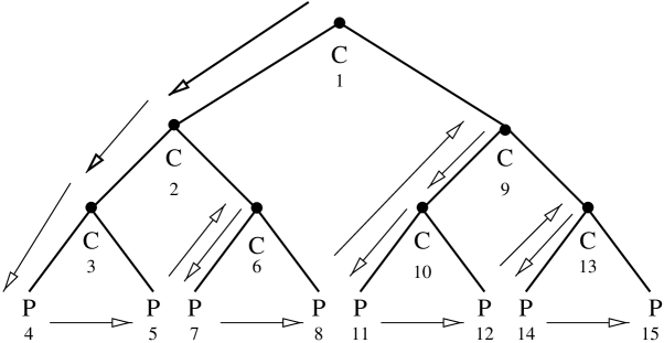
The first node in list is set to the root cell containing all of the particles. The descent of the tree always proceeds to the current node’s first child which is then added to the list. If the node contains only one particle the walk proceeds to the node’s sibling which is then added to the list. Once the nodes are sorted this way, a tree walk for a force calculation then reduces to a scanning of this list. If a cell must be opened, one simply examines the next node in this list which is guaranteed to be the first child cell at the next level of the hierarchy. If a cell can be used, the walk to the sibling is simply a jump down the list to the appropriate cell labelled by the sibling pointer. The other main advantage of resorting the tree nodes in this way is that it becomes easy to prune and graft trees onto existing structures which is essential in the parallelization of the code.

The BH tree algorithm as described above has been implemented on each processor in the parallel code. The node level code has been optimized using grouping and non-recursive tree walks and improve the tree code’s efficiency considerably over simpler versions.

3 Parallel Tree Codes

The parallelization of the BH algorithm is not obvious since the inhomogeneous distribution of particles in the oct-tree structure does not immediately lend itself to a simple domain decomposition with load balance. The main difficulty is that both the particles and the tree structure must somehow be distributed in a balanced way among many independent processors. Salmon (1990) describes one possible parallelization of the tree code which retains most of the features of the original tree code on the level of individual processors but introduces a new algorithm for distributing the particles and tree structure among the processors. We describe the algorithm below and its implementation on the CRAY T3D. The main difference between this new code and Salmon’s original code is the optimized implementation of the BH algorithm described in §2. The parallel features are essentially the same.

3.1 Orthogonal Recursive Bisection

In an N-body problem, the system of particles can be enclosed by a rectangular box for isolated systems like individual galaxies or an exact cube in cosmological systems with periodic boundaries. Salmon (1990) developed a parallel algorithm for decomposing this volume into rectangular sub-volumes using the method of orthogonal recursive bisection (ORB). In this technique, a volume is represented as a hierarchy of rectangular boxes somewhat like the BH tree. The main volume is first cut along an arbitrary dimension at an arbitrary position. For a balanced tree, the position is chosen so there are equal numbers of particles on each side of the cut. The resulting two volumes are cut again along the same or a different dimension again at an arbitrary position. The slicing of each subvolume continues for as many levels as required. The resulting process can be represented by a binary tree structure since each node points to two children. An ORB tree of $n$ levels therefore results in $2^{n}$ subvolumes. Most massively parallel computers are organized into partitions of $2^{n}$ processors ( $n\leq 10$ in practice) so that an $n$ -level ORB tree decomposition of an N-body volume maps conveniently onto a parallel machine.

At each level in the construction of the ORB tree, we have the freedom to choose both the dimension and position of the volume subdivision. For example, if the initial volume is a cube, one can construct a ORB tree analogue of the BH tree by cycling through the 3 dimensions and cutting only through the geometric center of each subvolume. However, with load balance in mind we wish to position our slice of the subvolume so that there are equal amounts of computational work on each side of the slice. This is the trick introduced by Salmon to achieve load balance. We can keep track of the computational work for an N-body simulation by simply summing up the number of cell-particle interactions, the main sink of computing time. In this way, once the particles in each subvolume are assigned to a processor, the calculation of the acceleration should be load balanced. Initially, the amount of computational work is unknown so it is assumed to be the same for each particle. The first step is therefore somewhat load imbalanced but in practice successive steps become more balanced.

The choice of dimension for cutting the subvolumes in the ORB tree construction is generally arbitrary but it is best to select the longest dimension for slicing. The tree code uses a multipole expansion to quadrupole order so we desire rectangular domains that are as “spherical” as possible.

An ORB domain decomposition on a parallel machine can be carried out by assuming the processors are layed out in a hypercube communication network. A machine containing $2^{n}$ processors can be arranged using the communication paradigm of an $n$ -dimensional hypercube. In this arrangement, each processor resides at the vertex of this hypercube and can only communicate to $n-1$ neighbors along the lines on the edge of the hypercube. A domain decomposition can be carried out in $n$ steps by consecutive exchanges of particles across the $n$ -dimensions of the hypercube network.

Processors are usually labeled by an integer between 0 and $2^{n}-1$ . If we represent processor $i$ in binary format, its hypercube partner across the $h$ th dimension is $i\;\;{\rm XOR}\;\;2^{h}$ where XOR is the logical exclusive-or operation. This has the effect of flipping the $h$ th bit from a 0 to 1 or vice versa. The ORB domain decomposition proceeds as follows. A position and dimension is selected for cutting the entire domain into two subdomains. For the first hypercube dimension, each processor exchanges particles with its unique partner so that all the particles in a given processor are on one or the other side of the first cut. After this first iteration, half of the processors contain particles on one side of the domain and half on the other. At each successive iteration, each subdomain finds the splitting position and dimension and processors once more exchange particles as above with their corresponding partner across the particular hypercube dimension. Finally, each processor contains its unique rectangular subdomain of particles (Figure 3).

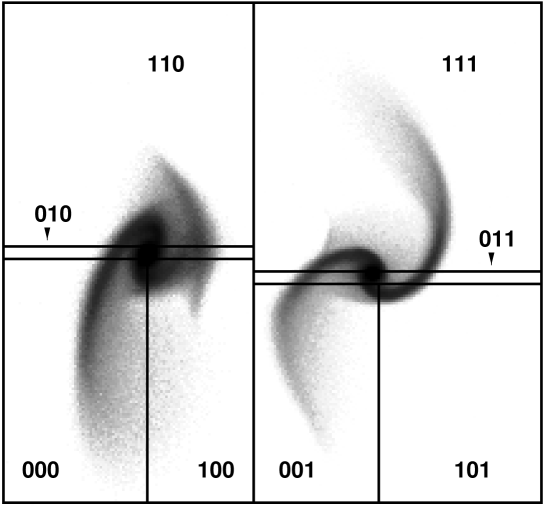
If the criterion for splitting domains is the amount of computational work, each processor also has an allotment of particles which will take roughly the same amount of computational effort. In practice, the memory imbalance can be substantial with some processors containing approximately twice as many particles as others although this has been found to be tolerable.

3.2 Linking the trees

After the domain decomposition, a BH tree can be constructed locally in each processor using the particles contained within its independent subvolume. After constructing the local trees, we would ideally like to link them together to form the full tree describing the entire system.

The top levels of the tree are simply the load-balanced ORB tree structure created by the domain decomposition, while the processors contain the BH trees (Figure 4). If a copy of this complete tree structure were available to each processor, they could proceed independently to evaluate the forces on their particles. Unfortunately, the amount of memory required for a full copy of the tree at each node is prohibitive.

Salmon (1990) solved this problem by introducing the concept of a locally essential tree. Each processor does not require an entire copy of the tree. Rather, only a significantly smaller subset of nodes is necessary since the BH-trees in distant volumes need only be opened to a lesser degree for all the particles in a given processor domain. The opening criterion can be applied to the entire group of particles in a processor by calculating the distance to the nearest edge of a processor volume in the same way as described above in the grouping scheme used to improve the efficiency of the force evaluations. Therefore, a processor only needs to import significantly pruned trees from distant processors which it can graft on to its existing structure to create the locally essential tree. This pruned tree of the entire system contains all the nodes required to calculate the forces to the required tolerance specified by the opening angle criterion.

In practice, the locally essential trees are constructed in the following manner. After building the local BH-tree, each processor imports the root nodes of the trees from all of the others in the pool (Figure 4). A local binary tree is built from the base up in each processor using the imported root nodes. A walk through the ORB tree using a group opening-criterion determines which subset of processors must be examined further to gather more tree nodes if necessary. Tree walks are performed in the needed processors using the group opening criterion of the requesting processors. BH tree nodes which can be used are flagged. The nodes of the pruned trees are then gathered together and exported to the calling processor. Once received the internal child and sibling links of the imported trees are reset and the pruned trees are grafted at the appropriate node of the ORB binary tree. The result of this procedure is the locally essential tree which contains: the local BH-tree, the ORB tree structure and the trees pruned to the appropriate levels imported from other processors.

3.3 Summary

In summary, the parallel tree code works as follows. At the start, particles are distributed randomly among the $2^{n}$ processors. At each timestep, the following procedures are carried out:

1.

ORB domain decomposition across processors.
2.

Construct the local BH tree.
3.

Exchange tree nodes to construct the locally essential trees.
4.

Walk through trees to calculate forces.
5.

Move particles along their trajectories using these forces.

Only steps 1. and 3. require message passing. In both cases, messages are exchanged in a synchronous manner using the hypercube paradigm described above. The messages contain arrays of particle data (masses, positions, and velocities) and tree node data (masses, positions, quadrupole moments and cell dimensions). To ease the problems of bookkeeping, the code is written in C and particle and tree node data are packaged in arrays of appropriate C structures. We use the Message Passing Interface (MPI) software to handle the message passing. The MPI functions are supported on almost all parallel machines so the code is portable to different platforms. The code runs on the Cray T3D, Intel Paragon, and the IBM SP/2.

4 Performance

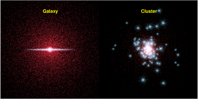
In this section, we describe some results on the code performance on the Cray T3D in terms of accuracy, speed and load balance. We use two test problems to profile the code: an isolated galaxy composed of a disk, bulge and a halo and a spherical cluster of galaxies following a Hernquist density profile. The first case represents a smooth centrally concentrated mass distribution expected in galaxy simulations while the second case exemplifies a strongly, inhomogeneous clustered distribution which arises in a cosmological context (Figure 5).

Tree codes usually run most slowly for these sorts of problems so the performance study here should test the code most rigorously. More homogeneous systems run approximately twice as quickly in practice. We note that the code has already been applied to simulations of interacting and colliding galaxies containing $\sim$ 300 thousand particles and runs without problems for greater than 1000 timesteps (Dubinski, Mihos, and Hernquist 1996). The code also runs on the Intel Paragon and the IBM SP2 and note that the performance on these machines is comparable to the T3D.

4.1 Acceleration Errors

We first measured the errors in acceleration, $|\delta{\bf a}|/|{\bf a}|$ , for various values of the cell opening angle, $\theta$ in single galaxy and cluster models. We only use a single processor to measure these errors. All cell-particle interactions are calculated to quadrupole order. The galaxy contained 40000 particle while the cluster contained 128 galaxies of $\sim 700$ particles each plus a smooth cluster dark halo for a total of 120000 particles. Accelerations were first calculated using $\theta=0.5$ . Since the errors are less than 0.02% for this case the accelerations are effectively exact for comparison to those calculated with larger values of $\theta$ . Figure 6 shows plots of the distribution of acceleration errors for various values of $\theta$ along with the resulting cumulative distribution.

Even with $\theta=1.2$ , the median error in the acceleration is still less than 0.5% while 90% of the measured accelerations are less than 1% for both the galaxy and the cluster. The addition of $\delta$ in Barnes’ new opening criterion causes many more cells to be opened than with the original criterion and therefore allows more accurate forces for larger values of $\theta$ . The old opening criterion gave similar error distributions for $\theta=1$ (Hernquist 1987).

We also found that as the number of processors increases, the mean acceleration errors are found to decline while the computing time per processor increases since more cell openings are required. The top cells of the tree in a multi-processor run created during the domain decomposition can have large aspect ratios (Figure 3). The result is more accurate forces than for a cubic decomposition since the walk through the hybrid ORB – BH tree structure must go to deeper levels than the pure BH tree to satisfy the cell-opening criterion. In principle, the extra accuracy is not needed but at least the slightly degraded performance results in a higher quality simulation.

4.2 Memory Requirements

The memory requirements of the parallel tree code are quite large. The majority of the memory is assigned to the particle and cell arrays in for the local subset of particles with additional arrays for particles and cells imported for the locally essential trees. The requirements for the particles and cells are respectively 15 and 20 machine words (8 bytes) with an additional arra for the tree nodes imported from other processors. The memory for imported tree nodes can increase substantially for small $\theta$ but in practice is $<$ 1 Megaword for $\theta>1$ in simulations that fully load the machine. In practice, there are about 6 Mwords available on the T3D for local particles and cells so this amounts to a maximum of 170K particles per processor. The scheme used for load-balancing computing time can lead to a memory imbalance of up to a factor of 2 in the number of particles per processor. The practical value for simulations is therefore about $\sim 100$ K particles per processor to allow for this imbalance. The memory is allocated and reallocated dynamically for added flexibility in managing the changing sizes of the particle and cell lists.

4.3 Timing

A successful parallel algorithm should have good load balance with a minimal overhead for processor communication. We ran our two test cases for a few time steps using different values of $\theta$ and different numbers of processors to examine these properties. We used larger number of particles to fully load the machines: 640 thousand particles for the galaxy, and 1.1 million for the cluster. We timed the computational functions (tree building/tree walking) and communication functions (domain decomposition and tree exchange and distribution) separately to measure the load balance and overall communication costs of the algorithm.

4.3.1 Load Balance

We define the load balance as:

B=\frac{\sum_{i}t_{i}+t_{c}}{{\rm max}(t_{1},t_{2},...,t_{n})+t_{c}}

(3)

where $t_{i}$ is the pure computational CPU time for a given processor and $t_{c}$ is the communication time. For this code $t_{c}$ is the same for each processor since message passing is done synchronously. The denominator is just the elapsed wall-clock time for each timestep. We define the communication overhead, $C$ , as the fraction of the total wall-clock time per step used for communication:

C=\frac{t_{c}}{{\rm max}(t_{1},t_{2},...,t_{n})+t_{c}}

(4)

The load balance and communication overhead for the test cases as a function of number of processors for are listed in Table 1. We show results for the first step and third step of an integration. In the first step, particles are assumed to have equal computational costs and are therefore arranged in an ORB tree with equal numbers of particles per processor. Load balance is in the range of 60%-70% while tolerable can still be improved considerably. We expect this first step to be poorly load balanced since we know that in practice particles will have a wide range of computational costs.

By the third step, the system is distributed by ORB according to computational load. For most cases, the load balance has improved considerably to greater than 90% for $n<64$ . The communication overhead is generally less than 10% of the total time per step so the computation is being dominated by physical calculations. For processor numbers greater than 128, there does not appear to be a major improvement in the load balancing by the third step. Communication costs become more significant and so the use of the number of cell interactions to estimate the load is not necessarily the best way to weight the particles. An additional term incorporating the communication cost in the load estimate may improve the balance. In any case, load balance is still better than 70% so there is not much room left for improvement.

Table 1
Load Balance
	Galaxy		Cluster
$n$	$B$	$C$	$B$	$C$
1st Step
16	0.77	0.03	–	–
32	0.71	0.04	0.85	0.06
64	0.66	0.09	0.84	0.12
128	0.64	0.16	0.87	0.28
256	0.69	0.32	0.87	0.38
3rd Step
16	0.95	0.04	–	–
32	0.95	0.06	0.93	0.04
64	0.92	0.09	0.94	0.06
128	0.80	0.12	0.93	0.11
256	0.73	0.21	0.88	0.15

4.3.2 Speed and Scaling

We first measured the speed of the code in terms of the number of particles which could be evaluated per second as a function of the number of processors. Speeds were calculated from the third step once the particles had settled into a load-balanced decomposition. The speed is simply, $S=N/t_{s}$ , where $N$ is the number of particles and $t_{s}$ is the elapsed wall-clock time per step. Figure 7 shows the code speed, $S$ , for various cases. The code shows an approximate linear scaling versus $n$ for $n<64$ but beyond that it falls off. As $n$ increases, the shapes of domains in the ORB decomposition have a larger range of aspect ratios forcing tree walks to proceed to deeper levels to satisfy the opening criterion. We found that the number of cell interactions grows with the number of processors because of this effect.

We also measured the speed simply as the number of cell interactions/second, the dominant source of computation, to see how well the raw computational speed of the code scales with $n$ . Figure 8 again shows a nearly linear scaling for $n<64$ after which there is a drop off which can be attributed mainly to the added load imbalance and communication cost for large $n$ . This speed is independent of the model for $n<64$ showing that it is an approximate measure of the raw computational speed. There are 72 floating point calculations per quadrupole order interaction plus one square root. There is also some computation associated with the tree walk and some direct particle-particle interactions. There are therefore approximately 100 floating point operations of useful work per cell interaction. The code speed on the T3D is therefore in the range of 15-20 MFlops/processor depending on $n$ . Similar estimates are found using the “Apprentice” profiling utility on the T3D. This value falls short of the peak theoretical speed of 150 MFlops/node. The deficit results from the large of amount of bookkeeping needed in shuffling and resorting particles and tree nodes at various times before actually doing the useful work of computing the forces.

In practice, the code running on a 16 node partition performs almost as well as Hernquist’s (1990) vectorized tree code on the CRAY C90. Walker’s 500,000 particle of satellite accretion ran at a rate of $\sim$ 4000 particles per second with $\theta=0.7$ (Walker, Mihos & Hernquist 1996). Parallel treecodes running on the newest parallel machines therefore offer about a factor of 10 fold increase in problem size or speed over vectorized tree codes.

We also note that the speed of this parallel code is comparable to Warren & Salmon’s (1994) when comparing their homogeneous sphere benchmarks.

5 Conclusions

A parallel tree code based on Salmon’s algorithm has been implemented using the MPI message passing software on 3 parallel machines: the Cray T3D, Paragon and the IBM SP/2. In principle, the code can also run on a small network of workstations although we have not had the opportunity to test it this way. The code incorporates an improved version of the BH tree algorithm including particle grouping for tree walks, non-recursive tree walking and a “safe” cell opening criterion. The code has been applied successfully to simulations of galaxy interactions (Dubinski, Mihos, & Hernquist 1996) and is currently being applied to a variety of other problems in galaxy dynamics.

The code works best with a small number of processors that are heavily loaded with particles. If $N<10^{6}$ , we find that the number of processors should be less than 64 to get the best use of computing time. Bigger problems will of course require the added memory of more processors.

This code’s main disadvantage is its excessive demand for memory. The memory needs become excessive when $\theta$ becomes too small. The use of locally essential trees is the main culprit in this respect. Perhaps, this method of load balancing can be replaced by an asynchronous message passing scheme in which tree walks in various processors are done on demand by distributing particles among the processors. At present, the code is still marginally time limited and available memory will be greater in the next generation of machines.

We are now in the process of adapting the code for both cosmological simulations with periodic boundary conditions and smoothed particle hydrodynamics (Dave, Dubinski & Hernquist 1996). With this new code, we should be able to increase the typical number of particles used in current CRAY C90 TREESPH (Hernquist & Katz 1989) simulation by a factor of 10-100. The improved dynamic range should allow simulations of galaxy formation in a full cosmological context.

I would like to thank Romeel Dave, Uffe Hellsten, Lars Hernquist and Guohong Xu for useful comments. I acknowledge grants for supercomputing time at the National Center for Supercomputing Applications, the Pittsburgh Supercomputing Center, the San Diego Supercomputing Center and the Cornell Theory Center.

references

Appel, A.W. 1985, In SIAM Journal on Scientific and Statistical Computing, 6, 85

Barnes, J. & Hut P. 1986, Nature, 324, 446

Barnes, J.E 1990, J. of Comp. Phys., 87, 161

Barnes, J.E. 1994, In Computational Astrophysics, Eds. J. Barnes et al. (Springer-Verlag: Berlin)

Benz, W., Bowers, R.L., Cammeron, A.G.W. & Press, W.H. 1990, ApJ, 348, 647

Bhatt, S.; Chen, M.; Lin, C.-Y.; Liu, P. 1992, In Proceedings Scalable High Performance Computing Conference (Los Alimitos: IEEE Comput. Soc. Press)

Dave, R., Dubinski, J. & Hernquist, L. 1996, in preparation

Dikaiakos, M.D. & Stadel, J. 1995, preprint

Dubinski, J. 1988, M.Sc. Thesis, University of Toronto

Dubinski, J., Mihos, J.C, & Hernquist, L. 1996, ApJ, in press

Fox, G.C., Williams, R.D, & Messina, P.C. 1994, Parallel Computing Works!, San Francisco, CA: Morgan Kaufmann Publishers Inc.

Hernquist, L & Katz, N. 1989, ApJS, 70, 419

Hernquist, L. 1987, ApJSS,, 64, 715

Hernquist, L. 1990, J. Comp. Phys., 87, 137

Hernquist, L., Bouchet, F.R., & Suto, Y. 1991, ApJSS, 75, 231

Hillis, W.D. & Barnes, J. 1987, Nature, 326, 27

Jernigan, J. G. & Porter, D. H 1989, ApJS, 71, 871

Makino, J. & Hut, P. 1989, Comput. Phys. Rep., 9, 199

Pal Singh, J. 1993, Ph. D. Thesis, Stanford University

Pal Singh, J., Holt, C., Totsuka, T., Gupta, A., & Hennessy, J. 1995, Journal of Parallel and Distributed Computing, 27, 118.

Salmon, J. 1990, Ph.D. Thesis, ”Parallel Hierarchical N-body Methods”, California Institute of Technology.

Salmon, J.K. & Warren, M.S. 1994, Journal of Computational Physics, 111, 136

Salmon, J.K., & Warren, M.S. 1994, International Journal of Supercomputing Applications, 8, 129

Steinmetz, M. & Muller, E. 1993, AA, 268, 391

Walker, I., Mihos, J.C. & Hernquist, L. 1996, ApJ, in press

Warren, M., and Salmon J. 1992, ApJ, 401,

Warren, M.S. 1994, Ph.D Thesis, Univeristy of California, Santa Barbara

Warren, M.S. & Salmon, J.K. 1993, In Proc. of Supercomputing ’93, 12