Numerical calculation of linear modes in stellar disks.

Abstract

We present a method for solving the two-dimensional linearized collisionless Boltzmann equation using Fourier expansion along the orbits. It resembles very much solutions present in the literature, but it differs by the fact that everything is performed in coordinate space instead of using action-angle variables. We show that this approach, though less elegant, is both feasible and straightforward.

This approach is then incorporated in a matrix method in order to calculate self-consistent modes, using a set of potential-density pairs which is obtained numerically. We investigated the stability of some unperturbed disks having an almost flat rotation curve, an exponential disk and a non-zero velocity dispersion. The influence of the velocity dispersion, halo mass and anisotropy on the stability is further discussed.

Key words: dynamics of galaxies – stability – structure of galaxies

The study of the perturbations in stellar disks (spirals and bars) has advanced along essentially 2 quite different avenues since the early 60’s.

Numerical N–body simulations probably offer the most flexible tools (e.g. [Hohl, 1971]; Athanassoula & Sellwood, 1986), they are relatively easily set up regardless the complexity of the initial conditions and include the description of nonlinear evolution. On the other hand, these simulations are very time-consuming and suffer from important, but hard to quantify, numerical noise.

A linearized self-consistent mode analysis, which explains linear instability during the onset, was the first method used, because initially N–body simulations were still essentially infeasible. This approach is somewhat complementary to N–body simulations. It heavily relies on simplifying assumptions but produces high quality results, of course only in the regions where the assumptions are valid. Although the literature offers general methods ([Kalnajs, 1977]) to calculate linear instabilities, these methods apparently are difficult to apply in practical situations. For this reason, several researchers have adopted further simplifications in order to handle the equations more conveniently, such as using cold disks with softened gravity ([Toomre, 1981]) and a gaseous approximation ([Bertin, Lin, Lowe & Thurstans, 1989]).

In this paper we develop an alternative method (section 2, 3 and 4), which resembles very much other approaches described in the literature (e.g. [Kalnajs, 1977], [Hunter, 1992]), but differs on a few important points. As in many other cases, the linearized Boltzmann equation is solved by fourier expansion of the perturbation along the unperturbed orbits. However, we perform all calculations in coordinate space instead of writing everything in action-angle variables. Despite the fact that the equations are less elegant, this strategy offers the advantage that the perturbed mass density as well as the full perturbed distribution is obtained in ordinary space and velocity coordinates. This considerably simplifies the solution of the Poisson equation, since any complete set of potential-density pairs is now sufficient to expand the perturbing potential. This is in contrast to the action-angle implementations, where usually bi-orthogonal sets enter the calculations (see Kalnajs (1977) for more details). In addition, the equations can be cast in such a form that all calculations are very efficient, since the evaluation of the response mass density is essentially reduced to the calculation of a Hilbert transform.

We applied this method to discuss the instabilities of a family of unperturbed disk models (described in section 1). All models feature a reasonably flat rotation curve and an exponential disk. This family consists of almost isotropic distribution functions, with varying velocity dispersions. Stability increases with increasing velocity dispersions and increasing halo mass (section 5). Section 6 sums up.

1 The models

Before presenting the method of the mode calculation in more detail, we first introduce the unperturbed galaxy models for which the calculations were performed. All our models have the same unperturbed potential and mass density, but feature different distribution functions, with varying velocity dispersion, streaming velocity and anisotropy.

1.1 The unperturbed potential

The potential of the unperturbed galaxy was constructed as a sum of two Kuzmin-Toomre disk potentials with different core radii. In the plane of the disk, it is given by

$$V_{0}(r)={1\over\sqrt{1+r^{2}}}+{1\over\sqrt{1+(r/4.4)^{2}}}.$$ (1)

Note that potentials are defined as binding energies, with a positive sign. This potential produces a rotation curve which is much flatter than a single component Kuzmin-Toomre potential (see fig. 1). The ratio of the flat part to the rising part is about $6/1$.

Fig. 1.: Rotation curve of the unperturbed galaxy potential

Although the rotation curve tends to rise somewhat too slowly near the centre, it has, at least qualitatively, a realistic behaviour.

1.2 The mass density profile

It is well-known that strongly flattened galaxies usually have a substantial amount of dark halo mass, extending much further than the visible component. It is sufficient for our purpose to model it by a spherical and pressure-supported galaxy component. Therefore it is reasonable to assume that this halo component only influences the stability behaviour of the disk by its contribution to the global potential. The same roughly holds for the central bulge, which is hot and has a three-dimensional structure as well. Thus both the halo and the bulge are “inert” and the corresponding potential and mass density are taken to be spherical and denoted by $V_{0,H}(r)$ and $\rho_{0,H}(r)$.

The disk itself is the only component which is supposed to consist of “active mass”, sensitive to instabilities. The unperturbed disk is supposed to be two-dimensional and axisymmetric, with a surface density $\rho_{0,D}$ and a potential $V_{0,D}$. We chose an exponential mass profile with a central core:

$$\rho_{0,D}=\alpha e^{-1.3\sqrt{0.2+r^{2}}}.$$ (2)

Although this mass density extends up to infinity, the actual models have an outer limit at $r=6$, and the mass density reaches zero at that point. This we achieve by fitting the distributions (2) with several finite components. The relative error made at the outer edge is only of the order of 0.1%. The parameter $\alpha$ determines the total disk mass.

Since the total system should be self-consistent, the total potential in the plane of the galaxy is given by the sum of the disk and halo component:

$$V_{0}(r)=V_{0,D}(r)+V_{0,H}(r).$$ (3)

Since the total potential $V_{0}$ has a fixed form (1) and the potential of the disk is determined by the surface mass density (2), we can calculate $V_{0,H}=V_{0}-V_{0,D}$. Thus follows the halo mass density

$$\rho_{0,H}=-{1\over 4\pi G}{1\over r^{2}}{d\over dr}\left(r^{2}{dV_{0,H}\over dr}\right),$$ (4)

and the total halo mass within a radius $r$

$$M_{0,H}(r)=-{1\over G}r^{2}{dV_{0,H}\over dr}.$$ (5)

Fig. 2.: Total mass inside $r$ of the disk (full curves) and the halo (dashed curves) for $H/D$=$2.5$, $5$ and $+\infty$.

Of course, the halo mass density should everywhere be positive. This puts an upper limit on the value of $\alpha$ in (2). The relative contribution of the disk and halo components are quantified using the halo-to-disk factor, $H/D$, which gives the proportion of the total mass inside the radius $r_{\rm max}$ (=6) for the halo and the active disk. Self-consistency with a non-negative spherical halo puts a lower limit on $H/D$ of about $2.5$. Note that the assumption of a spherical halo is not a crucial one. If one would assume an oblate halo, the only effect would be a somewhat lower minimum $H/D$.

1.3 The distribution function

We will examine the stability behaviour for different stellar distributions. According to Jeans’ theorem, the unperturbed part of the distribution is a function of two integrals of motion, the binding energy $E$ and the angular momentum $J$, defined by

$$E=V_{0}(r)-{1\over 2}(v_{r}^{2}+v_{\theta}^{2}){\rm\ \ \ and\ \ \ }J=rv_{\theta}.$$ (6)

In order to generate a variety of finite disks, based on the potential (1), the distribution function is written as a linear combination of basic distributions:

$$f_{0}(E,J)=\sum_{t=1}^{n_{t}}c_{t}f_{0,t}(E,J).$$ (7)

All components only have a (everywhere positive) contribution for orbits lying completely inside $r_{\rm max}$, i.e. for the region where (see also fig 16)

$$E\geq V_{0}(r_{\rm max})-{J^{2}\over 2r_{\rm max}^{2}},$$ (8)

$$E\geq V_{0}(r_{\rm max})-{1\over 2}v_{circ}^{2}(r_{\rm max}),$$ (9)

with $r_{\rm max}$ the radius of the edge of the disk. Equation (9) is required in order to exclude the region $r_{-}\geq r_{\rm max}$. In addition, the distribution goes to zero at this edge in a smooth way, so that the first derivative remains finite everywhere. The explicit form of the components is listed in the Appendix.

The expansion coefficients $c_{t}$ are determined by a least square fit of the corresponding mass density to the proposed exponential form (2) (the coefficients are forced to be positive, in order to avoid negative distributions). By choosing an appropriate set of components $f_{0,t}$, we were able to create the desired orbital densities. In all the models, the error on the fit to the mass density never exceeds 1% of the central value.

We constructed 4 models, labeled I to IV (the explicit form of the distribution functions is listed in the appendix). Along the sequence, the models become more and more rotation-supported, having an increasing streaming velocity and decreasing temperature. Fig. 3 shows the streaming velocities and dispersions for the coldest and hottest case. The dispersions all go to zero at the edge of the disk. Note that model I is perfectly isotropic and has a linearly increasing mean velocity curve. For all disks, Toomre’s local axisymmetric instability criterion ([Toomre, 1964])

$$Q={\sigma_{r}\kappa\over 3.36G\rho_{0,D}}$$ (10)

(with $\sigma_{r}$ the radial velocity dispersion and $\kappa$ the epicyclic frequency) is everywhere higher than $1$.

Fig. 3.: Streaming velocity (full line), azimuthal velocity dispersion (long dashed line) and radial velocity dispersion (short dashed line) for Model IV (top panel) and Model I (bottom panel).

In fig. 4, the distribution function of model III is shown in turning point space. The turning points of an orbit are the largest (resp. smallest) distance from the centre that an orbit can reach, and are called apocentre $r_{+}$, or pericentre $r_{-}$. By convention, we take $r_{+}$ always positive, while $r_{-}$ has the same sign as $J$. Evidently, these quantities are integrals of the motion and $r_{+}\geq|r_{-}|$ (on circular orbits, $r_{+}=r_{-}$). For a given pair $(r_{+},r_{-})$, the energy and angular momentum follow immediately from

$$E=V_{0}(r_{+,-})-{1\over 2}{J^{2}\over r_{+,-}^{2}},$$ (11)

which leads to

$$E={r_{+}^{2}V_{0}(r_{+})-r_{-}^{2}V_{0}(r_{-})\over r_{+}^{2}-r_{-}^{2}}$$ (12)

and

$$J=\sqrt{2}r_{+}r_{-}\sqrt{V_{0}(r_{+})-V_{0}(r_{-})\over r_{-}^{2}-r_{+}^{2}}.$$ (13)

Inversely, $r_{+}$ and $r_{-}$ are found as the roots for $r$ of (11) for a particular $E$ and $J$. We preferred these variables over the normal $(E,J)$ space, not only because they have an easy physical interpretation, but also because this representation is more related to our method for solving the linearized Boltzmann equation, which employs a grid interpolation in the turning point space (see following section).

We have chosen finite disks in order to compactify phase space. However, as can be seen from the distribution function (fig. 4), the disk reaches this limit at $r_{\rm max}$ in a very smooth way. This is important since it has been proven that a sharp edge or, more generally, a sharp feature in $(E,J)$ space, can introduce additional instabilities which might not always be physical ([Toomre, 1964], [Sellwood & Kahn, 1991]).

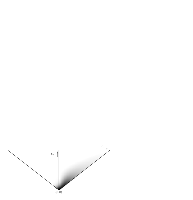
Fig. 4.: Turning point representation of the distribution function of model III.

2 The Poisson equation

Fig. 5.: Some of the lowest order potential-density pairs used to expand a general perturbation.

Since we want to study uniformly rotating perturbation modes, we suppose the following form for the perturbing potential:

$$V^{\prime}(r,\theta;t)=V^{\prime}(r)e^{i(m\theta-\omega t)}.$$ (14)

In this expression (and in all later similar expressions), only the real part corresponds to the physical quantity. There is no problem though to calculate with these complex expressions, since all equations are linear. This perturbation is rotating with a pattern speed of ${\rm Re}(\omega)/m$ and is exponentially growing with a growth factor ${\rm Im}(\omega)$. A more general pattern can be obtained as a superposition of such components with different $m$.

We will search for the linear modes using a matrix method, which requires a set of potential-density pairs suitable for the expansion of the perturbation. The literature offers a variety of analytical sets for infinite disks (eg. [Clutton-Brock, 1972], [Qian, 1993]) as well as for finite ones (eg. [Hunter, 1963]). The choice of a particular set largely depends on the structure of the unperturbed potential $V_{0}$ and density $\rho_{0}$. The importance of a suitable set of potential-densities is clearly illustrated by the displacement mode of a self-consistent disk. If the model has no inert halo component, a simple translation of the system is a valid “perturbation”. In linear theory, this corresponds to an $m=1$ mode of the form (see also section 4.1.3)

$${d\rho_{0}\over dr}(r)e^{i\theta}.$$ (15)

The potential-density pairs should of course be able to fit this behaviour well ([Weinberg, 1991]). Moreover, it is very important to choose the set as efficiently as possible, so that not too many expansion terms need to be calculated. For these reasons, we decided not to rely on existing analytical sets, but to create numerical sets which are tailor-made for the present unperturbed disk. If the maximum radius of the finite disk is denoted by $r_{\rm max}$, the set of densities for $m=0$ is given by

$$\rho^{0}_{S,n}(r)=\rho_{0,D}(r)*\cos(\pi n{r\over r_{\rm max}}),$$ (16)

and for $m>0$ by

$$\rho^{m}_{S,n}(r)=r^{m-1}{d\rho_{0,D}\over dr}(r)*\cos(\pi n{r\over r_{\rm max}}).$$ (17)

These densities have the right behaviour in the centre and at the edge of the galaxy. In addition, their number of radial nodes is equal to $n$. The corresponding potentials $V^{m}_{S,n}$ are easily calculated numerically using the integral form of the Poisson equation. These potential-density pairs prove to be very efficient for the expansion of the normal modes. Of course, these modes in principle could have been expanded using analytical complete sets described in the literature (e.g. [Hunter, 1963]), but this would require a long summation up to very high order, particularly because the density falls to zero very smoothly at the edge.

3 The linearized Boltzmann equation

3.1 Integral form

The total disk is modeled using two parts, a time-independent axisymmetric unperturbed part, and a small perturbation. Hence, the distribution function is written as

$$f(r,\theta,v_{r},v_{\theta};t)=f_{0}(E,J)+f^{\prime}(r,\theta,v_{r},v_{\theta};t),$$ (18)

while the total potential, which is defined as a binding energy (being positive everywhere), reads

$$V(r,\theta;t)=V_{0}(r)+V^{\prime}(r,\theta;t).$$ (19)

If the system is exposed to the perturbing potential $V^{\prime}$, the corresponding linearized response distribution is given by ([Vauterin & Dejonghe, 1995])

$$f^{\prime}={\partial f_{0}\over\partial E}f^{\prime}_{E}+{\partial f_{0}\over\partial J}f^{\prime}_{J},$$ (20)

where $f^{\prime}_{E}$ and $f^{\prime}_{J}$ satisfy (using Poisson brackets)

$${\partial f^{\prime}_{E}\over\partial t}-[f^{\prime}_{E},E]=[E,V^{\prime}]$$ (21)

and

$${\partial f^{\prime}_{J}\over\partial t}-[f^{\prime}_{J},E]=[J,V^{\prime}].$$ (22)

Integration with respect to the time along unperturbed orbits of both equations and expansion of the Poisson brackets immediately yields (since the left hand side is the total time derivative along an unperturbed orbit)

$$f^{\prime}_{E}(r^{0},\theta^{0},v_{r}^{0},v_{\theta}^{0};0) = \int_{-\infty}^{0}(v_{r}{\partial V^{\prime}\over\partial r}+{v_{\theta}\over r}{\partial V^{\prime}\over\partial\theta})dt$$ (23)

$$f^{\prime}_{J}(r^{0},\theta^{0},v_{r}^{0},v_{\theta}^{0};0) = -\int_{-\infty}^{0}{\partial V^{\prime}\over\partial\theta}dt.$$ (24)

The integrand is to be evaluated along the unperturbed orbit which passes at $t=0$ through the point $(r^{0},\theta^{0},v_{r}^{0},v_{\theta}^{0})$. One should note that these expressions can only hold if the perturbation was zero at $t=-\infty$ and is, at least infinitesimally, growing.

With a potential of the form

$$V^{\prime}(r,\theta,t)=V^{\prime}(r)e^{i(m\theta-\omega t)},$$ (25)

we have

$$f^{\prime}_{E} = \int_{-\infty}^{0}(v_{r}{dV^{\prime}\over dr}+imv_{\theta}{V^{\prime}\over r})e^{i(m\theta-\omega t)}dt$$ (26)

$$f^{\prime}_{J} = \int_{-\infty}^{0}imV^{\prime}e^{i(m\theta-\omega t)}dt.$$ (27)

These integrals are to be evaluated along unperturbed orbits, so one needs a way to handle such orbits.

3.2 Fourier expansion along unperturbed orbits

Since the unperturbed potential $V_{0}$ is axisymmetric, the corresponding orbital structure is particularly simple. Taking advantage of the conservation of angular momentum $J$, one can conclude that the radial coordinate behaves like the coordinate of a particle in a one-dimensional (so-called effective) potential

$$V_{\rm eff}(r)=V_{0}(r)-{J^{2}\over 2r^{2}}.$$ (28)

Supposed that the orbit is bound (which is the only case of interest for galaxies), the radial coordinate along an unperturbed orbit should be a periodic function of time, with angular frequency $\omega_{r}$. From this it follows immediately that $v_{r}$ and $v_{\theta}$ are periodic with frequency $\omega_{r}$ as well. As the mean value of $v_{\theta}$ should not necessarily be zero, the angular coordinate $\theta$ will be a superposition of a periodic function and a uniform “drift” velocity:

$$\theta=\omega_{\theta}t+\theta_{p}(t)$$ (29)

(with $\theta_{p}$ a periodic function with period $\omega_{r}$).

We will now rewrite the integrands of (26) and (27) by factorizing the part which is periodical with angular frequency $\omega_{r}$:

$$f^{\prime}_{E} = \int_{-\infty}^{0}I_{E}(t)e^{i(m\omega_{\theta}-\omega)t}dt$$ (30)

$$f^{\prime}_{J} = \int_{-\infty}^{0}I_{J}(t)e^{i(m\omega_{\theta}-\omega)t}dt,$$ (31)

with

$$I_{E}(t)=\left(v_{r}(t){\partial V^{\prime}\over\partial r}(t)+imv_{\theta}(t){V^{\prime}(t)\over r(t)}\right)e^{im\theta_{p}(t)}$$ (32)

and

$$I_{J}(t)=imV^{\prime}(t)e^{im\theta_{p}(t)}.$$ (33)

Since $I_{E}(t)$ and $I_{J}(t)$ are periodic, they can be expanded in Fourier series:

$$I_{E}(t)=\sum_{l=-l_{\rm max}}^{l_{\rm max}}I_{E,l}e^{il\omega_{r}t}$$ (34)

$$I_{J}(t)=\sum_{l=-l_{\rm max}}^{l_{\rm max}}I_{J,l}e^{il\omega_{r}t}$$ (35)

When these forms are substituted in (30) and (31), the integrations can be carried out analytically, at least if the perturbation is growing, ${\rm Im}(\omega)>0$. Note that, when the perturbation is decaying in time (${\rm Im}(\omega)<0$), one can still obtain a solution by performing the integrations (30) and (31) from $t=0$ to $t=+\infty$.

3.3 Grid interpolation

The Fourier expansion strategy yields the response distribution for any given perturbing potential, but a number of steps are involved even for calculating one single point of the distribution: the orbit should be integrated for at least one half of the radial period, and the appropriate functions are to be expanded in Fourier series. Since the perturbed distribution will be evaluated many times (e.g. for the calculation of the perturbed mass density one has to integrate over the velocities), it is absolutely necessary to be able to evaluate the response as fast as possible. Our solution is to calculate all appropriate parameters (the frequencies $\omega_{r}$ and $\omega_{\theta}$ and the Fourier expansions $I_{E,l}$ and $I_{J,l}$) on a (two-dimensional) grid in integral space and to store the result on disk for future use. We found that is was not so convenient to use $E,J$ as grid coordinates, since this grid is very inhomogeneous and has a relatively low density near the circular orbits, where disk galaxies have a dense population. Moreover, the circular orbit limit on this grid is usually not given in an analytic form. For these reasons, we used $r_{+}$ and $x=r_{-}/r_{+}$ as grid coordinates. In this representation, we can apply a simple rectangular grid which is very dense close to circular orbits and in the neighbourhood of the centre of the galaxy.

The $(r_{+},x)$ space is, up to the maximum radius $r_{+}=r_{\rm max}$, discretized using a rectangular grid. On each point of this grid, the Fourier expansion for the orbit starting at $t=0$ in its apocentre (by choice) is calculated and stored in a library, together with a tabulation of $t[r]$ and $\theta_{p}[r]$. In the following paragraphs, we will frequently use both the time and $r$–dependence of the same variable. In order to avoid confusing notations, $r$–dependences will be written using square brackets. The time and coordinate system is chosen in such a way that $\theta$ and $t$ are zero at the apocentre.

When the response distribution is later required in a point $p^{0}=(r^{0},\theta^{0}=0,v_{r}^{0},v_{\theta}^{0};t^{0}=0)$ in phase space, the corresponding turning points $r_{+}^{0}$ and $r_{-}^{0}$ are calculated and all parameters are interpolated using the four closest points on the grid (note that, since the response is a known periodic function of $\theta$, it is sufficient to evaluate it at $\theta=0$). In this way, we get an orbit out of the library with the correct integrals of motion, but passing through its apocentre at $t=0$. We will denote this library orbit and all corresponding quantities with a superindex $L$.

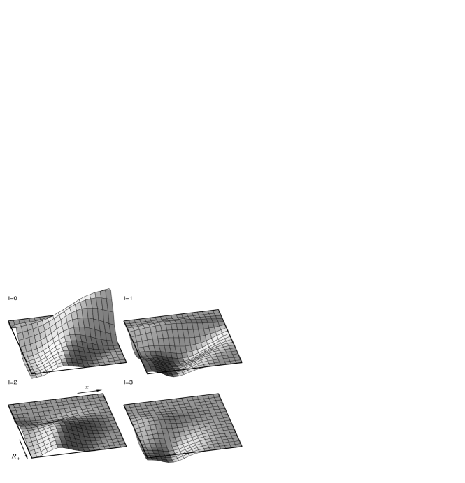
Fig. 6.: Interpolation grids of the lowest order Fourier coefficients for a $V_{S,1}^{2}$ perturbation (only the $x>0$ part is shown)

As the point $p^{0}$ is in general not the apocentre of the orbit, one should take in account an offset in time for the actual orbit passing through $p^{0}$:

$$I_{E}(t)=I_{E}^{L}(t+t^{L}[r^{0}]),$$ (36)

Note that $t^{L}[r^{0}]$ is actually a double–valued relation. However, the sign of $v_{r}^{0}$ can be used to determine which branch of the relation should be used. In general, there is also an offset in azimuth:

$$\theta(t)=\omega_{\theta}^{L}t+\theta_{p}^{L}(t+t^{L}[r^{0}])-\theta_{p}^{L}[r^{0}],$$ (37)

which is of course the reason why the functions $t[r]$ and $\theta_{p}[r]$ are stored. Note that the presence of these functions does not reduce the speed of the calculations, but implies only a slight increase in used disk space. The resulting perturbed distribution in that point follows then immediately:

$$f^{\prime}_{E}=\sum_{l=-l_{\rm max}}^{l_{\rm max}}{I_{E,l}^{L}e^{i(l\omega_{r}^{L}t^{L}[r^{0}]-m\theta_{p}^{L}[r^{0}])}\over i(l\omega_{r}^{L}+m\omega_{\theta}^{L}-\omega)}$$ (38)

and

$$f^{\prime}_{J}=\sum_{l=-l_{\rm max}}^{l_{\rm max}}{I_{J,l}^{L}e^{i(l\omega_{r}^{L}t^{L}[r^{0}]-m\theta_{p}^{L}[r^{0}])}\over i(l\omega_{r}^{L}+m\omega_{\theta}^{L}-\omega)}.$$ (39)

The Fourier coefficients which are stored on the grid only depend on the unperturbed and the perturbing potential. Furthermore, since the latter will be expanded in a basis, this has to be done only for the discrete set $V_{S,n}^{m}$. The orbits are obtained by integrating the system over half a period using a fourth order Runge-Kutta. Special attention should be paid to $r_{-}=0$ (or $J=0$) orbits, which have to be integrated in rectangular coordinates. In addition, since the Fourier coefficients are discontinuous at $r_{-}=0$ (see also [Kalnajs, 1977]), this should be performed twice, for “infinitesimally small” opposite values of $J$ in order to get the correct left and right limit.

The Fourier expansion is performed up to the order $l_{\rm max}=14$. This number should be relatively large in order to provide an accurate fit to the high excentricity orbits, which show fast variations close to the centre. A grid resolution of $60\times 60$ proved to provide more than enough accuracy, particularly because the functions do not show very steep gradients in the turning point space. In these circumstances and for a set of 8 perturbing potentials, the calculations take less than 4 hours on a 100 Specfp92 workstation. This work only has to be redone when one changes the unperturbed potential.

Fig. 6 shows some of the Fourier coefficient grids for a $m=2$ perturbing potential. It clearly illustrates that the higher order Fourier terms are only important for small $x=r_{-}/r_{+}$ and for large $r_{+}$, which means for very eccentric orbits. This indicates that, for relatively cool galaxies, a small number of Fourier terms can already yield reliable results.

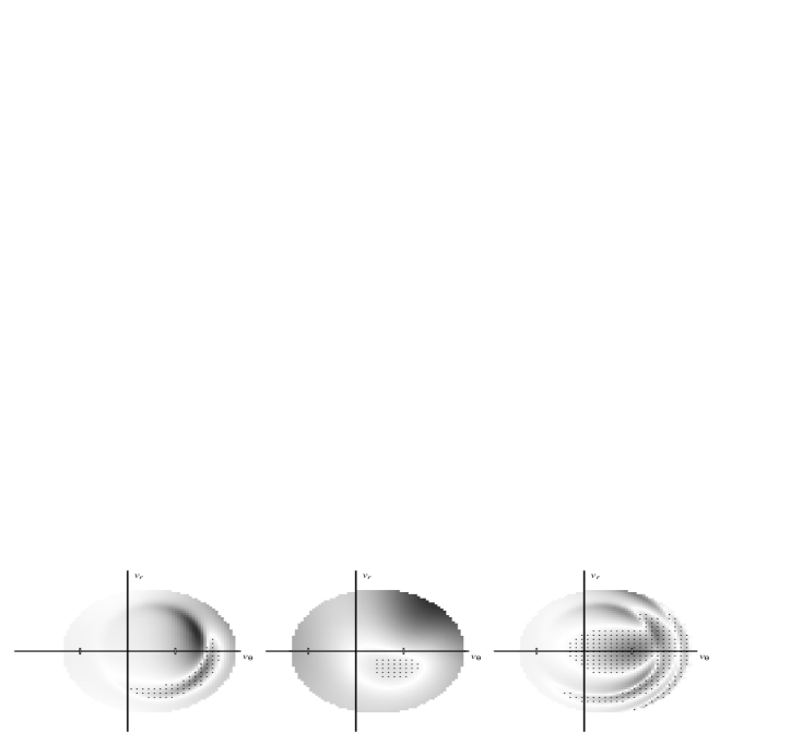
Fig. 7.: The real part of the perturbed distribution ${\rm Re}(f^{\prime}_{E})$ at $r^{0}=1.8$ for a typical $m=2$ perturbation. From left to right: at $\omega=(0.7,0.07)$, $\omega=(0.7,0.7)$ and $\omega=(1.5,0.1)$ (dotted regions are negative responses; the small ticks on the $v_{\theta}$ axis correspond to circular velocities).

Fig. 7 displays some response distribution functions for different $\omega$. The left and middle panels have the same pattern speed ${\rm Re}(\omega)/m$ and are taken somewhat inside the corotation radius. The left panel shows a response with a much smaller growth rate and therefore has a more prominent corotation resonance, appearing as a ring-shaped feature. This picture still has to be multiplied with $\partial f_{0}/\partial E$ which, for relatively cool disks, will emphasize the stars in the neighbourhood of circular orbits. One of the most crucial effects of non-zero velocity dispersion is that the distribution function populates stars on all possible orbits that are resonant with the perturbations, not only the resonances on circular orbits. These orbits fill a complicated region in phase space, cuts of which can be seen in velocity space in fig. 7. Due to the differential rotation, a substantial number of orbits at this radius are in corotation resonance, although this is not the corotation radius.

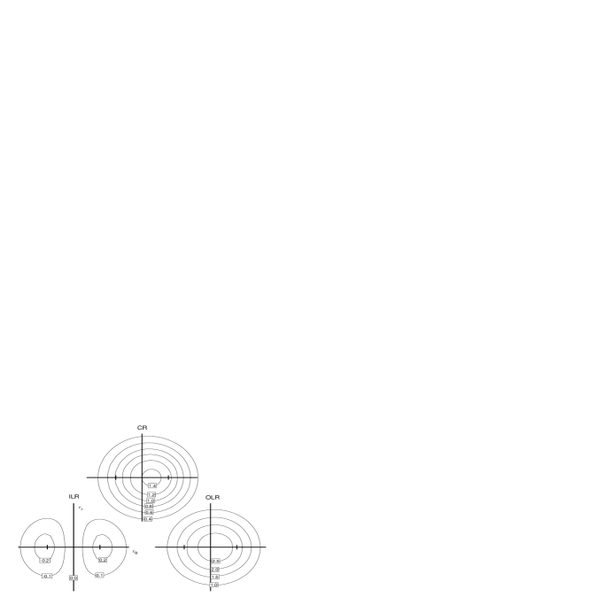
Fig. 8.: The resonant values of $\omega$ at $r=1$ in the $(v_{\theta},v_{r})$ plane for the three most important $m=2$ resonances. Circular velocities are indicated.

Fig. 8 shows, for a fixed radius, the velocity dependence of the resonant $\omega$ value for the dominant $m=2$ resonances. This value is given by

$$\omega=l\omega_{r}+m\omega_{\theta}.$$ (40)

The lowest order resonances for stars rotating in the direct sense ($\omega_{\theta}>0$) are $l$= $-1$ (ILR), $0$ (CR) and $1$ (OLR). However, there is a problem in this definition for counterrotating stars, since $\omega_{\theta}$ discontinuously changes its sign at $v_{\theta}=0$. This can be resolved by noticing that if, for counterrotating stars, $l$ is replaced by $l+m$ in (40), the resulting $\omega$ has an overall smooth behaviour. This is a consequence of the fact that for zero momentum stars $\omega_{r}=2\omega_{\theta}$. The ring-shaped CR position, as shown in fig. 8 (for varying $\omega$), can easily be found back in the left panel of fig. 7 (for a specific value of $\omega$).

Since $\omega_{r}$ and $\omega_{\theta}$ depend mostly on the energy $E$, the CR, OLR and higher resonances are roughly concentric circles around the origin. At the ILR though, the sum largely cancels out and result is mostly dominated by the angular momentum $J$.

3.4 Integration over the velocities

The method of the previous section can be used to calculate the perturbed distribution in a particular point of phase space $(r,\theta=0,v_{r},v_{\theta})$. Writing the velocities $(v_{r},v_{\theta})$ in polar coordinates $(v,\alpha)$, this results in a response

$$f^{\prime}(r,\theta=0,v,\alpha,t=0)=\sum_{l=-{l_{\rm max}}}^{l_{\rm max}}{A_{l}(r,v,\alpha)\over p_{l}(r,v,\alpha)-\omega},$$ (41)

with

$$p_{l}(r,v,\alpha)=l\omega_{r}+m\omega_{\theta}.$$ (42)

In order to obtain the perturbed mass density at a radius $r$ and for $\theta=0$, one has to integrate this expression over the velocities up to the escape velocity. Since the position of the pole $p_{l}$ in general depends also on the velocities, the denominator should be kept inside this integration:

$$\rho^{\prime}(r)=\sum_{l=-{l_{\rm max}}}^{l_{\rm max}}\int_{0}^{v_{esc}(r)}\int_{0}^{2\pi}{A_{l}(r,v,\alpha)\over p_{l}(r,v,\alpha)-\omega}vdvd\alpha.$$ (43)

In each term of the sum, we will switch the integration variables from $(v,\alpha)$ to $(p_{l}(r,v,\alpha),\alpha)$. The velocity then becomes a function $v=V_{l}(r,p_{l},\alpha)$ and the integral is written as

$$\rho^{\prime}(r)=\sum_{l=-{l_{\rm max}}}^{l_{\rm max}}\int_{p_{l,min}}^{p_{l,max}}{1\over p_{l}-\omega}dp_{l}\times$$

$$\int_{0}^{2\pi}A_{l}(r,V_{l}(r,p_{l},\alpha),\alpha)V_{l}(r,p_{l},\alpha){\partial v\over\partial p_{l}}(r,p_{l},\alpha)d\alpha.$$ (44)

The limits of the first integral can be chosen freely, as long as the interval is large enough to cover all poles. If $p_{l}(r,v,\alpha)$ is not a monotone function of $v$ over the entire region of interest, this transformation can still be performed by splitting up the integral in parts. There is a simple reason to write the expression in this way: for a constant $r$, the inner integrals are functions which only depend on $p_{l}$. If we sum all these functions over $l$ and denote this summation with $W(r,p)$, the perturbed mass density reduces to

$$\rho^{\prime}(r)=\int_{p_{\rm min}}^{p_{\rm max}}{W(r,p)\over p-\omega}dp,$$ (45)

which is a simple weighted integral over all real pole positions. This integral represents the Hilbert transform of $W$ with respect to $p$, assuming that $\rho$ is also a function of $\omega$. For each value of $r$, the function $W(r,p)$ can be tabulated and stored for later use. The evaluation of the perturbed density for any value of $\omega$ is then reduced to the numerical evaluation of a one-dimensional integral, which can be performed very fast.

Fig. 9.: The pole distribution $W(\omega)$ for the perturbed mass density using model III and a $V_{s,0}^{2}$ perturbation. The bumps at negative $p$ correspond to a counterrotating resonance.

In practice, $W(r,p)$ is not calculated using the explicit integral (44), because this would require the (piecewise) inversion of $p_{l}(v)$, which can be awkward. Instead, an alternative method is used, based on the two-dimensional integral (43). For any value of $r$, $W(p)$ is maintained in a tabular form, containing function values at fixed points with interleave $\Delta p$.

A numerical integration of the two-dimensional integral (43) is performed, using a rectangular grid over $[0,v_{\rm esc}]\times[0,2\pi]$, with interleaves $\Delta v$ and $\Delta\alpha$. In each cell of this grid, the integrand of (43) is approximately constant with respect to $v$ and $\alpha$. Therefore, the contribution of this cell to the integral is a pole function with respect to $\omega$, having a pole position $P=p_{l}(r,v,\alpha)$ and an amplitude $I=A_{l}(r,v,\alpha)v\Delta v\Delta\alpha$. This amplitude is now added to the table value of $W(p)$ that has a $p$ value lying closest to $P$. When all cells are summed, dividing all values in the $W(p)$ table by $\Delta p$ yields a numerical tabulation of $W(p)$. In practice, the summation over the cells is refined using a trapezoidal rule.

The values of the function $W(r,p)$ are stored on a grid containing 40 points in the $r$ dimension and $10^{4}$ points in the $p$ dimension, and the integral (45) is calculated by linear interpolation between the points in the $p$ dimension. However, one should be careful with values of $\omega$ lying in the neighbourhood of the real axis. If ${\rm Im}(\omega)$ is zero, the result is meaningless when $W(r,p)\neq 0$ in a region $[{\rm Re}(p)-\epsilon,{\rm Re}(p)+\epsilon]$ (in this case, stars are in resonance with a steady perturbation and the linear approximation breaks down anyhow). In addition, for such a region of non-zero weight for poles, $|{\rm Im}(\omega)|$ should be large in comparison with the grid distance of the $p$ grid in order to have a reliable interpolation. This is the reason why we take such a dense grid for $p$.

In fig. 9, the pole distribution $W(r,p)$ at various radii for a typical configuration is shown. For small $r$, the contributions of each resonance are easily distinguished, while for large $r$ the behaviour becomes more complex since the stars move slowly and many higher order resonances occur. This picture also clearly illustrates the non-localized character of the resonances, particularly for the corotation (CR) and outer Lindblad resonance (OLR). The inner Lindblad resonance (ILR) is, even for hot disks, much sharper, and remains roughly at the same value for $\omega$ throughout the galaxy. As noticed earlier ([Lin et al., 1969]), this interesting behaviour follows from the structure of the unperturbed potential. Due to this behaviour, the ILR plays a crucial role in the stability behaviour, even for high velocity dispersions.

Note that, for the panel corresponding with $r=1$, one can easily correlate the regions in $p$ spanned by the contributions of the individual resonances with the variation in $\omega$ shown by the corresponding contour plot in fig. 8.

4 Construction of normal modes

A matrix method is applied for searching the normal modes ([Kalnajs, 1977]). A general perturbing potential is written as

$$V^{\prime}=\sum_{i=0}^{s}a_{i}V^{m}_{S,i}.$$ (46)

Of course $s$ should be large enough so that all desired modes can be expanded accurately (the limitation on $s$ puts a limitation on the oscillatory behaviour of the modes).

Using the methods described in the previous paragraphs, the pole density functions $W_{S,i}^{m}(r,p)$ associated with the perturbing potentials $V^{m}_{S,i}$ are calculated and expanded as

$$W_{S,i}^{m}(r,p)=\sum_{j=0}^{s}\bar{c}_{j,i}^{m}(p)\rho_{S,j}^{m}.$$ (47)

This expansion is obtained using a least square fit. One can easily obtain $\bar{c}_{j,i}^{m}(p)$ in tabular form by performing the fit on each of the rows in the $r$ direction of the $W(r,p)$ grid. We can now write the response density ${\rho^{\prime}}^{m}_{S,i}$ for each of the potentials $V^{m}_{S,i}$ as

$${\rho^{\prime}}^{m}_{S,i}=\sum_{j=0}^{s}c_{j,i}^{m}(\omega)\rho^{m}_{S,j},$$ (48)

if we define

$$c_{j,i}^{m}(\omega)=\int_{p_{min}}^{p_{\rm max}}{\bar{c}_{j,i}^{m}(p)\over\omega-p}dp.$$ (49)

The response potential of (46) now follows immediately:

$$\sum_{j=0}^{s}\left(\sum_{i=0}^{s}c_{j,i}(\omega)a_{i}\right)V^{m}_{S,j}.$$ (50)

For a self-consistent mode, this response should be equal to the original perturbing potential (46). So the search for normal modes is reduced to the search for those values of $\omega$ for which the matrix $C(\omega)$ (with elements $c_{q,p}$) has a unity eigenvalue $\lambda$. The corresponding eigenvector gives the expansion of the normal mode.

Fig. 10.: Real and imaginary part of the multi-valued eigenvalue relation $\lambda(\omega)$ at ${\rm Im}(\omega)=0.11$ for the model III. The different kinds of lines correspond to different branches of the relation. The unique eigenvalue with $\lambda=1$ is indicated.

A typical situation for the multi-valued eigenvalue relation $\lambda(\omega)$ is shown in fig. 10. The steep edge in ${\rm Re}(\lambda)$ and the sharp peak in ${\rm Im}(\lambda)$ at small positive pattern speeds are the dominating features and are caused by the ILR because the reaction of the disk is strongest at ILR (see also fig. 9). For each value of ${\rm Im}(\omega)$ and for each branch, there appears to be only one (small and positive) value of ${\rm Re}(\omega)$ where ${\rm Im}(\lambda)$ is zero. The value of ${\rm Re}(\lambda)$, which decreases for increasing ${\rm Im}(\omega)$, further determines the mode location.

Obviously this search for unity eigenvalues in the complex plane has to be performed numerically. This is the main reason why we put so much emphasis on the development of a method to evaluate $C(\omega)$ as fast as possible. It takes less than a second to calculate the eigenvalues for a particular $\omega$, using an expansion up to an order $s=8$. Due to the efficient structure of the potential–density pairs, this limit is certainly sufficient for an accurate expansion of the unstable modes, since they prove to be of a relatively low order. The program calculates a detailed numerical tabulation of the complete dispersion relation in a sufficiently large region of the complex plane. This tabulation is further used to determine all modes using a binary intersection algorithm. This whole procedure takes less than one hour.

4.1 Checkpoints

Of course, there is a strong need for good checkpoints before starting to interpret the results coming out of this method. We checked the system in three ways, together covering more or less the whole chain of operations. The positive results of these checks are not only a good indication that the calculations are not obviously wrong, but they provide a good tool to determine the values of the various parameters (grid resolutions, expansion limits, …) in order to get results with sufficient accuracy. Most of these parameters were actually determined experimentally, using these test cases.

4.1.1 Comparison with direct integration

For a given perturbing potential, the linearized Boltzmann equation can be integrated numerically, at least for sufficiently fast growing perturbations. This yields values for the perturbed distribution function which should be the same as those coming from the Fourier expansion along the orbits.

4.1.2 Uniformly rotating disks

In a previous paper ([Vauterin & Dejonghe, 1995]), the mode analysis for uniformly rotating disks has already been performed in an independent way. If the same models are treated using the present approach, the same results should come out.

4.1.3 The displacement mode

As mentioned already, for models without passive component, a simple displacement of the disk is a valid “perturbation” ([Weinberg, 1991]). In a linear approach, the responses corresponding to this mode are obtained by derivation of the unperturbed values with respect to a rectangular coordinate (e.g. $x$). For the unperturbed mass density, this results in (using the fact that $x=re^{i\theta}$)

$${\partial\rho_{0,D}\over\partial x}(r)={\partial\rho_{0,D}\over\partial r}(r)e^{i\theta}.$$ (51)

The distribution function gives rise to the following perturbation:

$$f^{\prime}={\partial f_{0}\over\partial E}{\partial E\over\partial x}+{\partial f_{0}\over\partial J}{\partial J\over\partial x},$$ (52)

so that we immediately have that

$$f_{E}^{\prime}={\partial E\over\partial x}={dV_{0}\over dr}e^{i\theta},$$ (53)

and

$$f_{J}^{\prime}={\partial J\over\partial x}=v_{y}=(v_{\theta}-iv_{r})e^{i\theta}.$$ (54)

We used a self-consistent model based on a single Kuzmin-Toomre potential to prove that the method is able to find such modes. Note that, although this displacement mode occurs at $\omega=0$, there is no problem with the resonances since the pole distribution $W(r,0)=0$ for $m=1$ perturbations, which we verified numerically.

5 Results and discussion.

We performed the linear mode analysis for the models I to IV. These models have a roughly isotropic distribution function, with a velocity dispersion which is decreasing from model I to model IV. The aim of this set of models is to address the dependence of the stability on two important parameters, the velocity dispersion and the halo to disk proportion, $H/D$. Both parameters are now widely believed to have a crucial impact on the stability. The velocity dispersion of a particular model will be represented by its central value, $\sigma_{\rm cent}$, which is a good estimator of the relative overall behaviour (see fig. 3). Unstable modes with $m$ varying from $0$ to $4$ were sought in all models and for varying $H/D$. One can easily obtain the results for different $H/D$ simply by varying the total magnitude of the unperturbed distribution function, represented by $\alpha$ in (2).

Fig. 11.: Instability limits in the $\sigma_{\rm cent}$ vs. $H/D$ plane (taken as ${\rm Im}(\omega)=0.005$) for the lowest order modes in models I to IV. The lower left corner corresponds to unstable regions. The models are represented by small circles, and the model number decreases from the left to the right (the lines between the models are cubic spline interpolations).

In fig. 11, the stability limits for these modes are plotted in the $\sigma_{\rm cent}$ vs. $H/D$ plane (we chose ${\rm Im}(\omega)=0.005$ as a stability limit, since ${\rm Im}(\omega)=0$ is unreachable with our method). These curves were obtained by a cubic spline interpolation between the four models, which are represented by small circles. For most of the modes, only a small fraction of the models can actually reach the unstable regime. The other models only become unstable if they are combined with a spherical halo which is not everywhere positive (and hence $H/D<2.5$). The curves in figure 11 and 12 are always interpolations between all four models, but many models appear under the $H/D=2.5$ limit.

The region under each curve is the unstable region. At every point of the figure, the actual (in)stability of the disk is of course determined by the highest limit. Not surprisingly, the disk is effectively stabilized by increasing the velocity dispersion or by adding mass to the inert halo, or a combination of both. This behaviour has already been reported for various other cases, such as Kuzmin potentials ([Sellwood, & Athanassoula, 1986], [Athanassoula & Sellwood, 1986]) and quadratic potentials ([Vauterin & Dejonghe, 1995]). Another feature, which was also shown to be present in quadratic potentials, is that the slope of the stability limits increases for increasing $m$ (at least for $m\geq 2$). For hot disks, the $m=2$ mode is the only unstable one, while at the cool end, $m=4$ turned out to be the most unstable perturbation. Note that the model I was found to be stable for all calculated harmonics.

Fig. 12.: Contour lines of the growth rate of the dominating $m=2$ mode as a function of $\sigma_{\rm cent}$. The small circles represent the model points (the lines connecting the models are interpolations). The dotted line is an extrapolation at ${\rm Im}(\omega)=0$, and is the same as the height $m=2$ limit in fig. 13.

The growth rate for the most unstable $m=2$ mode is shown in fig. 12, again as a function of $\sigma_{\rm cent}$ and $H/D$. This picture clearly shows that the growth rate tends to increase in a more than linear way as the halo mass decreases. There is also a tendency that the contour lines become less dependent on the velocity dispersion for large values of the growth rate. This can be understood from the fact that varying the velocity dispersion re-distributes the weights $W(p)$ of the pole positions, and does not change the overall intensity (which is influenced by the factor $H/D$). When ${\rm Im}(\omega)$ becomes large, the pole distribution is “seen” from a big distance, and the internal positions become less important than the overall intensity.

Fig. 13.: Growth rate of the $m=2$ mode as a function of Toomre’s $Q$ factor in the centre of the galaxy.

Athanassoula and Sellwood (1986) suggest that a value of $2.0$-$2.5$ for Toomre’s local stability parameter $Q$ might by a useful criterion for stability of the disk against global $m=2$ perturbations. For the present models, fig. 13 plots the growth rate of the dominant $m=2$ mode against the corresponding $Q_{\rm cent}$, the value in the centre of the galaxy. As $Q$ is an increasing function of the radius, $Q_{\rm cent}$ is a lower limit of any averaging of $Q$ over the disk. For each model, the variation in $Q$ is obtained by changing $H/D$. Equation (10) shows that $Q$ simply scales with $\rho_{0}$, which is influenced by $H/D$. The figure shows that a value between $2.0$ and $2.4$ is indeed again a good estimation of the stability limit. Our values are slightly larger than those of Sellwood & Athanassoula, but this can be explained by the fact that they used a softened gravity.

Fig. 14.: Pattern speed of the perturbation as a function of the growth rate. The dashed horizontal line corresponds to the limit of the presence of an ILR.

The pattern speed of the perturbation, given by ${\rm Re}(\omega)/m$, is plotted against the growth rate in fig. 14 (note that ${\rm Im}(\omega)=0$ is, again, an extrapolation). This curve is shown for the three unstable models II, III and IV, and the variation in the growth rate is obtained by varying $H/D$. The endpoints of these curves are a consequence of the self-consistency requirement. The pattern speed has a clear increasing correlation with the growth rate, which is again in agreement with N-body simulations ([Athanassoula & Sellwood, 1986]). In addition, this figure shows that, for the same growth rate, the pattern speed decreases with the velocity dispersion. On the same picture, the upper limit on the pattern speed for the presence of an ILR is shown as a horizontal line. From this, it is clear that none of our models have an ILR, again in agreement with the results decribed by Athanassoula & Sellwood (1986). In fact, orbits which are in ILR cause such a violent response (see e.g. fig. 9 and fig. 10) that it would be very hard for a galaxy to maintain much of them.

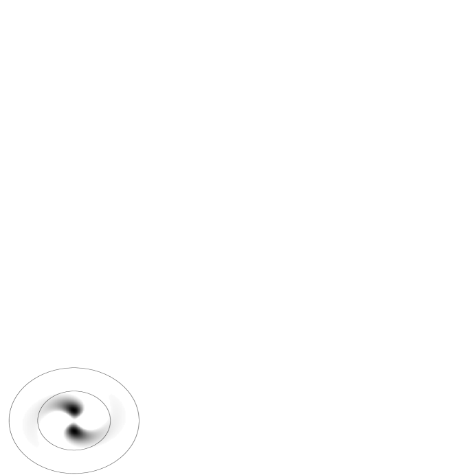
Fig. 15.: Dominating $m=2$ mode for the model III at $H/D=2.5$. The two circles correspond to the CR and OLR. Both the streaming velocity and the pattern speed are clockwise.

As a matter of illustration, fig. 15 shows the density profile of the dominating $m=2$ mode in model III. This perturbation develops its usual behaviour, with a bar-shaped central part and losely wound spiral arms in the outer regions. The spiral structure is always found to be trailing.

6 Conclusions.

A big part of this article was devoted to the description of a method for finding linear modes in stellar disks. The proposed strategy heavily relies on existing techniques, such as the matrix method and Fourier expansion along the unperturbed orbit, but differs from previous approaches by the fact that everything is calculated in ordinary coordinate and velocity space and that a numerical set of potential-density pairs is used. With the proposed scheme, the full perturbed distribution function is obtained with no extra calculation costs. In this way we have shown that calculations in coordinate space, although much less suited for theoretical considerations, can offer a fast and flexible alternative to action-angle variables when it comes to numerical computation of normal modes.

This method was applied to a set of unperturbed disk models, having a more or less realistic potential and an exponential mass density. This disks are embedded in a spherical, inert halo in order to obtain a self-consistent model. In agreement with various other studies (e.g. [Athanassoula & Sellwood, 1986]; [Vauterin & Dejonghe, 1995]), the calculations showed that these disks can be stabilised by increasing the velocity dispersion and/or the halo mass. For almost isotropic velocity dispersions, a $Q_{cent}$ value of $2.0-2.5$ turned out to be a reasonable stability limit.

Comparison of the stability of the present models with the behaviour of disks embedded in quadratic potentials ([Vauterin & Dejonghe, 1995]) shows a striking resemblance. Qualitatively, the stability behaviour of those simple uniformly rotating systems shares all the features that we have found for the more sophisticated models discussed in this paper. And, to a certain degree, there is even a quantitative agreement. It seems that, for some important aspects of the stability behaviour, the structure of the unperturbed distribution might be more inportant than the nature of the unperturbed potential.

Acknowledgements. The authors wish to thank the referee, C. Hunter, for a thorough reading of the manuscript and the many valuable comments. P. Vauterin acknowledges support of the Nationaal Fonds voor Wetenschappelijk Onderzoek (Belgium)

A The unperturbed distribution functions.

The simple $r_{+}=r_{max}$ limit of the unperturbed distribution in phase space, defined in $E$-$J$ space by

$$E_{L}(E,J)=E+{J^{2}\over 2r_{max}^{2}}-V_{0}(r_{max})\geq 0.$$ (A1)

is not so well suited for rotating models, since it is completely symmetric with respect to $J$. Therefore we have chosen for an alternative limit with the same zeroth and first derivative as $E_{L}$ at the point of the circular orbits with $r=r_{max}$ and with positive $J$, but with a second derivative which can be chosen freely. It is defined by

$$E_{L,\beta}(E,J)=E-E_{c,max} + {J_{c,max}\over r_{max}^{2}}(J-J_{c,max})$$ (A2)

$$- \beta(J-J_{c,max})^{2}\geq 0,$$

with the binding energy for circular orbits with positive $J$ at $r_{max}$

$$E_{c,max}=V_{0}(r_{max})+{1\over 2}r_{max}{dV_{0}\over dr}(r_{max}),$$ (A3)

and the angular momentum at the same point

$$J_{c,max}=r_{max}\sqrt{-r_{max}{dV_{0}\over dr}(r_{max})}.$$ (A4)

The parameter $\beta$ is adjustable. For large $r$, this new limit lies closely to circular orbits with positive $r$, and is much better suited for rotating models. In order to avoid unwanted orbits with $r_{+}>r_{max}$, both limits (A2) and (A3) should be combined with the extra condition (see also figure 16)

$$E\leq E_{c,max}.$$ (A5)

The unperturbed models are defined as

$$f_{\rm I}=E_{L,0.0}\times(\qquad 3.84\times 10^{-3} E^{4}$$ .

$$+2.22\times 10^{-1} 1\qquad),$$ . (A6)

$$f_{\rm II}=E_{L,0.007}\times(\qquad 3.68\times 10^{-2} E^{4}$$ .

$$+3.15\times 10^{-1} E^{4}{\rm pw}(J,2)\qquad),$$ . (A7)

$$f_{\rm III}=E_{L,0.01}\times(\qquad 5.69\times 10^{-4} E^{11}e^{4J}$$ .

$$+7.69\times 10^{-2} E^{8}{\rm pw}(J,2)$$ .

$$+1.40\times 10^{-1} E^{6}{\rm pw}(J,4)\qquad),$$ . (A8)

$$f_{\rm IV}=E_{L,0.01}\times(\qquad 6.69\times 10^{-8} E^{25}e^{9J}$$ .

$$+7.90\times 10^{-6} E^{25}{\rm pw}(J,2)$$ .

$$+7.54\times 10^{-3} E^{20}{\rm pw}(J,5)$$ .

$$+4.29\times 10^{-2} E^{14}{\rm pw}(J,7)\qquad).$$ . (A9)

The function ${\rm pw}(x,n)$ which we introduced equals $x^{n}$ for $x>0$ and zero for $x\leq 0$. If $n$ is integer and larger than one, this function has a continuous first derivative.

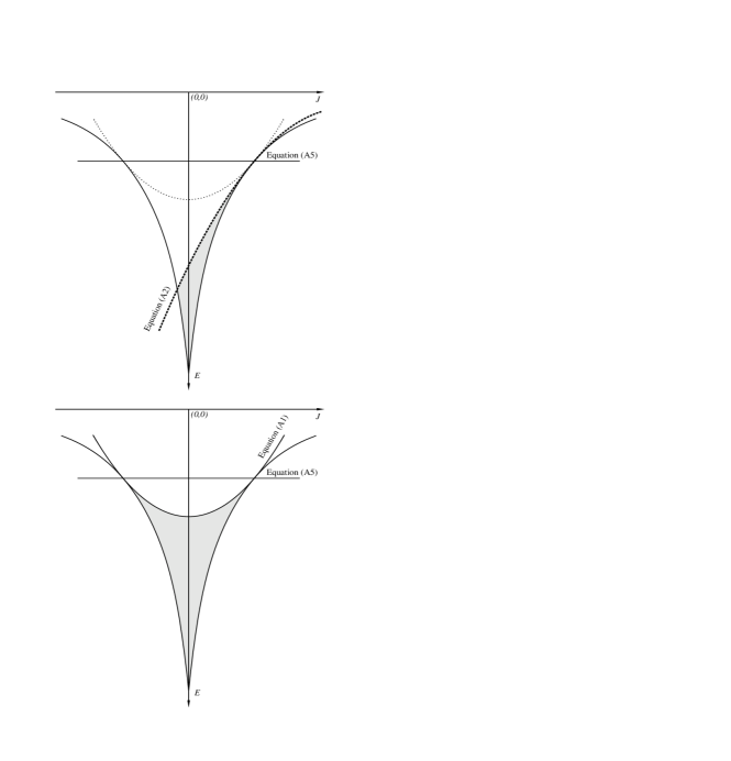
Fig. 16.: Representation of the orbits in $E$–$J$ space. The shaded region contains the allowed orbits. The functional dependence of the two limiting curves is given in the text. Top: limits used for the present models. Bottom: simple $r_{+}\leq r_{\rm max}$ limits.

References

- Athanassoula & Sellwood, 1986 Athanassoula, E., Sellwood, J. A., 1986, MNRAS, 221, 213
- Bertin, Lin, Lowe & Thurstans, 1989 Bertin, G., Lin, C. C., Lowe, S. A., Thurstans, R. P., 1989, ApJ, 338, 78
- Binney & Tremaine, 1987 Binney, J., Tremaine, S., 1987, Galactic Dynamics, Princeton University Press.
- Clutton-Brock, 1972 Clutton-Brock, M., 1972, Astr. & Spa. Sc., 16, 101
- Hunter, 1963 Hunter, C., 1963, MNRAS, 126, 299
- Hunter, 1992 Hunter, C., 1992, in: Astrophysical Disks, ed. S.F. Dermott, J.H. Hunter and R.E. Wilson (New York Academy of Sciences)
- Hohl, 1971 Hohl, F., 1971, Astrophys. Sp. Sc., 14, 91
- Kalnajs, 1977 Kalnajs, A. J., 1977, ApJ, 212, 637
- Lin et al., 1969 Lin, C.C., Yuan, C. & Shu, F.H., 1969, ApJ, 155, 721
- Qian, 1993 Qian, E. E., 1993, MNRAS, 263, 394
- Sellwood, & Athanassoula, 1986 Sellwood, J. A., Athanassoula, E., 1986, MNRAS, 221, 195
- Sellwood & Kahn, 1991 Sellwood, J. A., Kahn, F. D., 1991, MNRAS, 250, 278
- Toomre, 1964 Toomre, A., 1964, ApJ, 139, 1217
- Toomre, 1981 Toomre, A., 1981, In Structure and evolution of normal galaxies, eds. S. M. Fall & D. Lynden-Bell, Cambridge University press, 111
- Vauterin & Dejonghe, 1995 Vauterin, P., Dejonghe, H., 1995, A & A, in press
- Weinberg, 1991 Weinberg, M. D., 1991, ApJ, 368, 66