Observability of secondary Doppler peaks in the CMBR power spectrum by experiments with small fields

Abstract

We investigate the effects of finite sky coverage on the spectral resolution $\Delta\ell$ in the estimation of the CMBR angular power spectrum $C^{\ell}$. A method is developed for obtaining quasi-independent estimates of the power spectrum, and the cosmic/sample variance of these estimates is calculated. The effect of instrumental noise is also considered for prototype interferometer and single-dish experiments. By proposing a statistic for the detection of secondary (Doppler) peaks in the CMBR power spectrum, we then compute the significance level at which such peaks may be detected for a large range of model CMBR experiments. In particular, we investigate experimental design features required to distinguish between competing cosmological theories, such as cosmic strings and inflation, by establishing whether or not secondary peaks are present in the CMBR power spectrum.

1 Introduction

The cosmic microwave background radiation (CMBR) is one of the most promising links between astronomical observation and cosmological theory. A significant amount of experimental data already exists and further observational progress is expected in the near future. The experimental success in this field has prompted a large amount of theoretical effort on two closely related fronts. Firstly, theorists strive to assess the impact current observations have on theories of the early Universe. Secondly, the design of future experiments is guided by what are believed to be crucial tests of our theoretical prejudices.

A particularly active field of research in CMBR physics are the so-called Doppler peaks (Hu & Sugiyama 1995a,b). These consist of a series of oscillations in the angular power spectrum of CMBR fluctuations $C^{\ell}$ predicted for most inflationary models. They are predicted in the multipole range $100\la\ell\la 1500$, corresponding to angular scales $0.05\la\theta\la 1$ degrees. Experimental measurement of the Doppler peaks’ positions and heights would fix at least some combinations of cosmological parameters (e.g. $H_{0}$, $\Omega_{0}$ etc.) which are left free in inflationary models (Jungmann 1995). Future experimental projects are usually designed with these goals in mind. In particular, models with $\Omega_{0}=1$ are of special interest.

In this paper we shall consider another theoretical context. For a long time inflation (Steinhardt 1995), and topological defects (Kibble 1976; Vilenkin & Shellard 1994), have stood as conceptually opposing alternative scenarios for structure formation in the early Universe. It was shown by Albrecht et al (1996) and Magueijo et al (1996), that qualitative aspects of Doppler peaks should reflect this conceptual opposition. In particular the absence of secondary Doppler peaks was proved to be a robust prediction for a large section of defect theories. Interestingly enough this statement relies only on the role played by causality and randomness in these theories. Cosmic strings were unambiguosly shown to fall in this category. However, this may or may not be the case for textures (Crittenden & Turok 1995; and Durrer et al 1995). Therefore it appears that determining whether or not there are secondary Doppler peaks in the CMBR power spectrum offers an important alternative motivation for experimental design and data analysis. Answering this question is a far less demanding experimental challenge, which nevertheless will have a dramatic impact on our understanding of the Universe (Magueijo & Hobson 1996, Albrecht & Wandelt 1996).

We address this issue by proposing in Section 5 a statistic for detecting secondary oscillations, and studying how it fares for signals coming from various models, when measured by using different experimental strategies. The result is encoded in a detection function $\Sigma$ telling us to within how many sigmas we can claim a detection of secondary oscillations, given a particular model and experiment. We consider signals coming from standard CDM (sCDM), and an open CDM model (henceforth called stCDM) which is tuned to confuse inflation and cosmic strings in all but the issue of secondary oscillations. In Secs. 2, 3, and 4 we set up a framework for computing errors in power spectra estimates. We consider errors resulting from spectral resolution limitations due to finite sky coverage, cosmic/sample variance, instrumental noise and foreground subtraction. We consider a large parameter space of experiments including single-dish experiments and interferometers. For single-dish experiments we allow the beam size, sky coverage, and detector noise to vary. For interferometers we take as free parameters the primary beam, number of fields, and detector noise. We then use this framework to compute the detection function $\Sigma$ for sCDM and stCDM in this large class of experiments.

The results obtained are given in Sections 5 and 6, and provide experimental guidance in two different ways. Firstly they allow the choice of an ideal scanning strategy (choice of resolution and sky coverage) given a constraint such as finite funding (albeit disguised in a more mathematical form). Secondly, one may compute the expected value of the detection, assuming ideal scanning, as a function of available funding. This provides lower bounds on experimental conditions for a meaningful detection as well as an estimate of how fast detections will improve thereafter. We summarize the main results in the Section 7.

2 Observations of small fields

CMBR temperature fluctuations are usually described as an expansion in spherical harmonics

$$\frac{\Delta T(\mn@boldsymbol{\hat{x}})}{T}=\sum_{\ell=0}^{\infty}\sum_{m=-\ell}^{\ell}a_{\ell m}Y_{\ell m}(\mn@boldsymbol{\hat{x}}),$$

from which we define the CMBR power spectrum $C^{\ell}=\langle|a_{\ell m}|^{2}\rangle$. Note that in this paper we write ensemble average quantities with the indices upstairs, and denote observed values of such variables in any given experiment with the indices downstairs.

If one is looking only at small patches of the sky, the spherical harmonic analysis is awkward to apply, and it is more convenient to use Fourier analysis. For that purpose we perform a stereographic projection of the celestial sphere onto a tangent plane at the centre of our small patch, so that circles with colatitude $\theta$ are mapped onto circles of radius $r=2\tan(\theta/2)$ on the plane. We can then describe the CMBR fluctations $\Delta T(\mn@boldsymbol{x})/T$ on this plane by its Fourier transform. We use the conventions

$${\Delta T(\mn@boldsymbol{x})\over T}={\int{d^{2}\mn@boldsymbol{k}\over 2\pi}a(\mn@boldsymbol{k})e^{i\mn@boldsymbol{k}\cdot\mn@boldsymbol{x}}}\;,$$

and

$$a(\mn@boldsymbol{k})={\int{d^{2}\mn@boldsymbol{x}\over 2\pi}{\Delta T(\mn@boldsymbol{x})\over T}e^{-i\mn@boldsymbol{k}\cdot\mn@boldsymbol{x}}}.$$

If we denote the Fourier transform of the autocorrelation function of the $\Delta T(\mn@boldsymbol{x})/T$ field by $C(\mn@boldsymbol{k})/(2\pi)$ then the covariance of the Fourier modes $a(\mn@boldsymbol{k})$ is given by

$$\langle a(\mn@boldsymbol{k})a^{*}(\mn@boldsymbol{k}^{\prime})\rangle=C(k)\delta(\mn@boldsymbol{k}-\mn@boldsymbol{k}^{\prime}),$$ (1)

where the angle brackets denote ensemble averages, * denotes complex conjugation and $k=|\mn@boldsymbol{k}|$. We note that, due to the requirement of rotational invariance, $C(\mn@boldsymbol{k})=C(k)$. From (1), the raw modes $a(\mn@boldsymbol{k})$ are therefore independent Gaussian random variables with variance $C(k)$. In calculations concerning small patches of the sky $C(k)$ can be obtained by interpolating the $C^{\ell}$ coefficients in the spherical harmonic expansion with $|\mn@boldsymbol{k}|=\ell$ (Bond & Efstathiou 1987). An improvement can be obtained with the prescription $C(k)=C[\ell(k)]dk/dl$ with $k(\ell)=\pi\cot(\pi/\ell)$.

We wish to study the statistical properties of the $a(\mn@boldsymbol{k})$ modes as seen by observations of a small field with a given observing beam. Let us describe the field by a window $W(\mn@boldsymbol{x})$ and the observing beam by $B(\mn@boldsymbol{x})$. The sampled temperature map for a single-dish experiment is then

$${\Delta T_{s}(\mn@boldsymbol{x})\over T}=\left[{\Delta T(\mn@boldsymbol{x})\over T}\star B(\mn@boldsymbol{x})\right]W(\mn@boldsymbol{x}),$$

where $\star$ denotes convolution. The sampled Fourier modes $a_{s}(\mn@boldsymbol{k})$ are therefore given by

$$a_{s}(\mn@boldsymbol{k}) = [a(\mn@boldsymbol{k})\widetilde{B}(\mn@boldsymbol{k})]\star\widetilde{W}(\mn@boldsymbol{k})$$ (2)

$$= \int{d^{2}\mn@boldsymbol{k}^{\prime}\over 2\pi}\widetilde{W}(\mn@boldsymbol{k}-\mn@boldsymbol{k}^{\prime})a(\mn@boldsymbol{k}^{\prime})\widetilde{B}(\mn@boldsymbol{k}^{\prime}),$$

where $\widetilde{W}(\mn@boldsymbol{k})$ and $\widetilde{B}(\mn@boldsymbol{k})$ denote the Fourier transforms of the window and observing beam respectively.

For interferometers, however, we must make a slight modification since in this case the Fourier domain is sampled directly. An interferometer samples the Fourier transform of the product of the sky temperature fluctuations and the primary beam of the antennas $W(\mn@boldsymbol{x})$ (which corresponds to a window). The positions of these samples (or visibilities) in the Fourier domain (or $uv$-plane) are determined by the physical positions of the antennas and the direction to the patch of sky being observed, and lie on a series of curves (or $uv$-tracks). If we denote these curves by the function $\widetilde{B}(\mn@boldsymbol{k})$, which equals unity where the Fourier domain in sampled and equals zero elsewhere, then the sampled Fourier modes for an interferometer are given by

$$a_{s}(\mn@boldsymbol{k}) = [a(\mn@boldsymbol{k})\star\widetilde{W}(\mn@boldsymbol{k})]\widetilde{B}(\mn@boldsymbol{k})$$ (3)

$$= \widetilde{B}(\mn@boldsymbol{k})\int{d^{2}\mn@boldsymbol{k}^{\prime}\over 2\pi}\widetilde{W}(\mn@boldsymbol{k}-\mn@boldsymbol{k}^{\prime})a(\mn@boldsymbol{k}^{\prime}).$$

The inverse Fourier transform of $\widetilde{B}(\mn@boldsymbol{k})$ is the synthesised beam of the interferometer $B(\mn@boldsymbol{x})$. The $a_{s}(\mn@boldsymbol{k})$ modes are often inverse Fourier transformed to make a sky map. This sampled sky temperature distribution for an interferometer is

$${\Delta T_{s}(\mn@boldsymbol{x})\over T}=\left[{\Delta T(\mn@boldsymbol{x})\over T}W(\mn@boldsymbol{x})\right]\star B(\mn@boldsymbol{x}),$$

which is the convolution of the synthesised beam with the product of the sky and the primary beam (or window).

From (1), (2) and (3) one can then derive the covariance matrix of the sampled modes for each experiment (Hobson, Lasenby & Jones 1995). For a single-dish observation we find

$$\langle a_{s}(\mn@boldsymbol{k})a_{s}^{*}(\mn@boldsymbol{k}^{\prime})\rangle=$$

$$~{}~{}~{}~{}\int{d^{2}\mn@boldsymbol{k}^{\prime\prime}\over(2\pi)^{2}}\widetilde{W}(\mn@boldsymbol{k}-\mn@boldsymbol{k}^{\prime\prime})\widetilde{W}^{*}(\mn@boldsymbol{k}^{\prime}-\mn@boldsymbol{k}^{\prime\prime})C(\mn@boldsymbol{k}^{\prime\prime})|\widetilde{B}(\mn@boldsymbol{k}^{\prime\prime})|^{2},$$ (4)

whereas for an interferometer

$$\langle a_{s}(\mn@boldsymbol{k})a_{s}^{*}(\mn@boldsymbol{k}^{\prime})\rangle=$$

$$~{}~{}~{}~{}|\widetilde{B}(\mn@boldsymbol{k})|^{2}\int{d^{2}\mn@boldsymbol{k}^{\prime\prime}\over(2\pi)^{2}}\widetilde{W}(\mn@boldsymbol{k}-\mn@boldsymbol{k}^{\prime\prime})\widetilde{W}^{*}(\mn@boldsymbol{k}^{\prime}-\mn@boldsymbol{k}^{\prime\prime})C(\mn@boldsymbol{k}^{\prime\prime}).$$ (5)

Ignoring, for the moment, the effects of the observing beam $B(\mn@boldsymbol{x})$ in each case, we see that finite sky coverage [described by the window $W(\mn@boldsymbol{x})$] renders the observed $a_{s}(\mn@boldsymbol{k})$ dependent random variables. Roughly speaking, if $L$ is the typical size of the field then a correlation length $\xi\approx 1/L$ is introduced in the $\mn@boldsymbol{k}$-plane.

2.1 The sampled power spectrum

The two-dimensional sampled power spectrum may be defined in terms of the marginal variances of the sampled modes as

$${\sf C}^{s}(\mn@boldsymbol{k})=\langle a_{s}(\mn@boldsymbol{k})a_{s}^{*}(\mn@boldsymbol{k})\rangle$$

From (4) and (5) we see that ${\sf C}^{s}(\mn@boldsymbol{k})$ is given for single-dish experiments by

$${\sf C}^{s}(\mn@boldsymbol{k}) = \int\frac{d^{2}\mn@boldsymbol{k}^{\prime}}{(2\pi)^{2}}|\widetilde{W}(\mn@boldsymbol{k}-\mn@boldsymbol{k}^{\prime})|^{2}C(\mn@boldsymbol{k}^{\prime})|\widetilde{B}(\mn@boldsymbol{k}^{\prime})|^{2}$$ (6)

$$= \left[C(\mn@boldsymbol{k})|\widetilde{B}(\mn@boldsymbol{k})|^{2}\right]\star|\widetilde{W}(\mn@boldsymbol{k})|^{2},$$

and for interferometers by

$${\sf C}^{s}(\mn@boldsymbol{k}) = |\widetilde{B}(\mn@boldsymbol{k})|^{2}\int\frac{d^{2}\mn@boldsymbol{k}^{\prime}}{(2\pi)^{2}}|\widetilde{W}(\mn@boldsymbol{k}-\mn@boldsymbol{k}^{\prime})|^{2}C(\mn@boldsymbol{k}^{\prime})$$ (7)

$$= |\widetilde{B}(\mn@boldsymbol{k})|^{2}\left[C(\mn@boldsymbol{k})\star|\widetilde{W}(\mn@boldsymbol{k})|^{2}\right].$$

Ignoring, for the moment, the effects of the observing beam $B(\mn@boldsymbol{x})$ [by setting its Fourier transform $\widetilde{B}(\mn@boldsymbol{k})$ to unity in (6) and (7)], we see that in both cases the two-dimensional sampled power spectrum is the convolution of the underlying CMBR power spectrum $C(k)$ with $|\widetilde{W}(\mn@boldsymbol{k})|^{2}$. We also note that in general ${\sf C}^{s}(\mn@boldsymbol{k})$ is not circularly symmetric. We therefore define the one-dimensional sampled power spectrum as the azimuthal average $C^{s}(k)=\langle{\sf C}^{s}(k,\theta)\rangle_{\theta}$, where $\theta$ is the azimuthal angle in the Fourier domain.

In order to provide examples of the effects of the window on the sampled power spectrum, we now consider two simple windows: a square window and a Gaussian window. A square window is a toy model for single-dish experiments. If the square window has sides of length $L$, then its Fourier transform is given by

$$\widetilde{W}(\mn@boldsymbol{k})={L^{2}\over 2\pi}j_{0}\left({k_{x}L\over 2}\right)j_{0}\left({k_{y}L\over 2}\right),$$ (8)

where $j_{0}(x)=\sin x/x$ is the spherical Bessel function of order zero. A Gaussian window normalized to one at its peak is a toy model for an inteferometer primary beam, and is given by

$$W(\mn@boldsymbol{x})=\exp\left(-\frac{x^{2}}{2\sigma_{w}^{2}}\right),$$

which has the Fourier transform

$$\widetilde{W}(\mn@boldsymbol{k})=\sigma_{w}^{2}\exp\left(-\frac{k^{2}\sigma_{w}^{2}}{2}\right).$$

We note that both the square and Gaussian windows are real, even functions, and hence so are there Fourier transforms.

Using these windows we may now calculate the sampled power spectrum for various experiments (assuming for the moment that $\widetilde{B}(\mn@boldsymbol{k})=1$), given an underlying CMBR power spectrum. We choose the underlying spectrum to be that predicted by the standard inflation/CDM scenario with $\Omega_{0}=1$, $h_{0}=0.5$, and $\Omega_{b}=0.05$ (which we shall call sCDM). In order to accentuate the effects of the windows we first consider small fields.

As a model single-dish experiment we consider a square field of size $L=1.8$ degrees observed with a Gaussian beam with $\sigma_{w}=0.06$ degrees (or FWHM equal to 0.14 degrees), so that

$$\widetilde{B}(k)=\exp\left(-\frac{k^{2}}{2k_{b}^{2}}\right),$$ (9)

where $k_{b}=1000$. For a square window the two-dimensionsal sampled power spectrum is not circularly symmetric, and so ${\sf C}^{s}(k,\theta)$ is a function of $\theta$. If we fix $\theta=\theta_{0}$ for any value of $\theta_{0}$ in the range $[0,2\pi]$, we find that the spectrum starts as white-noise, i.e. ${\sf C}^{s}(k,\theta_{0})=\lambda$ for some constant $\lambda$, up to $k_{\rm min}\approx 2\pi/L$. From that point on, a spurious set of oscillations with period $\approx 4\pi/L$ appear superposed on the raw spectrum. This illustrated in Fig. 1 in which we plot ${\sf C}^{s}(k,0)$. The spurious oscillations merely reflect the ‘ringing’ of the Fourier transform due to the sharp edges of the window. In the 1-dimensional azimuthal average power spectrum $C^{s}(k)={\langle{\sf C}^{s}(k,\theta)\rangle}_{\theta}$ these spurious oscillations are mainly smoothed out, but so too are features in the raw spectrum on scales less than $\Delta\ell\approx 4\pi/L$ (see Fig. 11).

Figure 1: (Top) The sampled power spectrum ${\sf C}^{s}(k,0)$ (dashed line) for a single beam experiment with a square window of size $L=1.8$ degrees and resolution $k_{b}=1000$, compared to the underlying sCDM power spectrum (solid line) as observed by an all sky experiment with the same resolution. (Bottom) The same as above but for the azimuthal average sampled power spectrum $C^{s}(k)=\langle{\sf C}^{s}(k,\theta)\rangle_{\theta}$.

It is well-known (e.g. Press et al 1994) that the spurious oscillations in Fourier transforms can be suppressed by multiplying the data (sky map) by a window that goes to zero smoothly at its edges. In the context of CMB measurements, Tegmark (1996) calculates the optimal window to use in various circumstances to obtain the highest possible $\Delta\ell$ resolution in the sampled power spectrum. For a square field this window is a cosine ‘bell’

$$W(\mn@boldsymbol{x})=\cos\left(\frac{\pi x}{L}\right)\cos\left(\frac{\pi y}{L}\right),$$ (10)

whose Fourier transform is

$$W(\mn@boldsymbol{k})={2\pi\over L^{2}}{\cos{(k_{x}L/2)}\over k_{x}^{2}-(\pi/L)^{2}}{\cos{(k_{y}L/2)}\over k_{y}^{2}-(\pi/L)^{2}}.$$ (11)

At any given point $k_{0}$ in the sampled power spectrum this window minimises the variance (second central moment) $\langle(k-k_{0})^{2}\rangle$ of the convolving function $|\widetilde{W}(\mn@boldsymbol{k})|^{2}$. Interestingly, the more commonly encountered Hann window

$$W(\mn@boldsymbol{x})=\frac{1}{2}\left[1+\cos\left(\frac{2\pi x}{L}\right)\right]\left[1+\cos\left(\frac{2\pi y}{L}\right)\right],$$

minimises the fourth central moment $\langle(k-k_{0})^{4}\rangle$ of the convolving function.

Using the cosine bell window (10), the spurious oscillations disappear from ${\sf C}^{s}(k,0)$ and $C^{s}(k)$, but for such a small field the features of the raw spectrum are still heavily smeared (see Fig. 2).

Figure 2: As in Fig. 1 but for a square multiplied by a cosine bell.

For interferometers we may model the window (primary beam) as Gaussian. In Fig. 3 we show the effect on the sampled power spectrum of a Gaussian window with $\sigma_{w}=0.6$ degrees, which corresponds to a FWHM of 1.3 degrees. Although for a real interferometer observation, $\widetilde{B}(\mn@boldsymbol{k})=1$ only where the Fourier domain is sampled (and is zero elsewhere), in order to illustrate the effect of the window we set it equal to unity for all $\mn@boldsymbol{k}$. In Fig. 3, we again observe a white-noise tail up to $k_{\rm min}\approx 1/\sigma_{w}$, but from then on the Gaussian window does not induce spurious oscillations on the spectrum. The Gaussian window (which occurs naturally for inteferometer observations) is in fact quasi-optimal, and the procedure suggested by Tegmark (1996) makes a negligible difference to the spectral resolution of the sampled power spectrum. However, this window is still too narrow since features in the underlying spectrum on the scale of $\mbox{few}\times 1/\sigma_{w}$ are smoothed out. Hence although Gaussian windows do not distort smooth spectra, they still erase oscillations in oscillatory spectra if the window is too small. In Fig. 3 we show that effect of the Gaussian window on CMBR power spectra predicted by sCDM and cosmic strings (Magueijo et al 1995).

Figure 3: (Top) The sampled power spectrum (dashed line) observed by an experiment with a Gaussian window with $\sigma_{w}=0.6$ degrees, compared to the underlying CMBR spectrum predicted by cosmic strings (solid line). (Bottom) The same as above, but for the sCDM spectrum.

Therefore, for particularly small fields ($\la 2$ degrees), the sampled power spectrum $C^{s}(k)$ is a bad estimator for the underlying CMBR power spectrum $C(k)$, even after smoothing out field edge effects. However, in spite of the examples given, as the size of the field increases the sampled power spectrum rapidly converges to the underlying power spectrum for $k>k_{\rm min}$. In fact so long as edge effects are dealt with, for fields as small as 10 degrees for a square window (with cosine bell applied) or 5 degrees FWHM for a Gaussian window, the sampled power spectrum $C^{s}(k)$ faithfully reflects the underlying Doppler peak structure (see for instance Fig. 5). For these fields, apart from the white-noise tail for $k<k_{\rm min}$, one then has

$${\sf C}^{s}(\mn@boldsymbol{k})\approx\alpha C(k)|\widetilde{B}(\mn@boldsymbol{k})|^{2},$$

where the normalisation constant $\alpha$ is given by

$$\alpha=\int{d^{2}\mn@boldsymbol{k}\over(2\pi)^{2}}|\widetilde{W}(\mn@boldsymbol{k})|^{2}=\int{d^{2}\mn@boldsymbol{x}\over(2\pi)^{2}}|W(\mn@boldsymbol{x})|^{2}\equiv{\Omega_{s}\over(2\pi)^{2}}.$$ (12)

Equation (12) defines the effective solid angle $\Omega_{s}$ of the sampled field. In the previous plots $C^{s}(k)$ was divided by $\alpha$ to give the correct normalisation.

2.2 Correlations in the sampled power spectrum

As we have seen, finite fields have the effect of distorting the underlying CMBR power spectrum by convolving it with the function $|\widetilde{W}(\mn@boldsymbol{k})|^{2}$. Aside from smoothing the underlying power spectrum, this convolution also has the effect of inducing correlations between the values of the sampled power spectrum $C^{s}(k)$ for different values of $k$. To investigate these correlations further, we must first consider the correlations induced in the sampled Fourier modes $a_{s}(\mn@boldsymbol{k})$.

We expect correlations to exist between neighbouring sampled Fourier modes within some correlation length $\xi$. However, if the window has sharp edges, and the raw $C(k)$ spectrum falls-off as $1/k^{2}$ or slower at low $k$, then in addition to nearby correlations there are also ‘resonant’ long range correlations even for relatively large fields. We illustrate this point by considering the correlation of sampled modes around a given circle in $\mn@boldsymbol{k}$-space, i.e. ${\rm cor}[a_{s}(k,0),a_{s}(k,\theta)]$ as a function of $\theta$ for some given radius $k$. This quantity may be easily calculated from from (4) or (5), and is plotted in Fig. 4 for $k=50$ for various windows.

For an inteferometer observation with a Gaussian window the correlations fall-off at a correlation length of order $\xi\approx 1/\sigma_{w}$ around each mode. Furthermore, there are no long-range (anti-)correlations, and indeed no anti-correlations whatsoever. For single-dish observations with a square window, however, apart from correlations between neighbouring modes up to $\xi\approx 1/L$, there also exist ‘resonant’ anti-correlations between modes symmetric about the origin. This effect only disappears for $k>k_{b}/2$, where $k_{b}$ defines the angular resolution of the single-dish observation as in (9). This behaviour may be suppressed by multiplying the field by a cosine bell, as discussed above, and the result is also shown in Fig. 4.

Figure 4: The correlation of sampled Fourier modes ${\rm cor}[a_{s}(50,0),a_{s}(50,\theta)]$ as a function of $\theta$: (top) for a Gaussian window with $\sigma_{w}=12$ degrees; (bottom) for a square window with $L=36$ degrees (solid line), and same field but multiplied by a cosine bell (dashed line). Correlations fall-off beyond $\theta\approx 1/\sigma_{w}$ or $\theta\approx 1/L$, except for fields with sharp edges, where long distance correlations persist. In particular, for a square window there exist large anticorrelation between modes symmetric about the origin of $\mn@boldsymbol{k}$-space.

The correlations between Fourier modes strongly affect power spectra estimation. Let us consider the observed sampled power spectrum

$$C_{s}(k)={\int^{2\pi}_{0}}{d\theta\over 2\pi}|a_{s}(k,\theta)|^{2},$$ (13)

(which in keeping with our notation we write with the $s$ downstairs). Although $\langle C_{s}(k)\rangle=C^{s}(k)$ (as expected), the correlation of the Fourier modes induces correlations between $C_{s}(k)$ and $C_{s}(k^{\prime})$ for $|k-k^{\prime}|<\xi$. These correlations are troublesome as they may impart features on any observed spectrum $C_{s}(k)$ which average out to zero in the ensemble average spectrum $C^{s}(k)$. This renders $C_{s}(k)$ a bad estimator for $C^{s}(k)$, and conversely makes $C^{s}(k)$ a poor prediction for what an observers actually sees. For example, as we show later, the low $k$ white noise tail $C^{s}(k)=\lambda$ (for some constant $\lambda$) corresponds to a single correlated piece of the spectrum. As a result a typical observer does not see a spectrum $C_{s}(k)\approx\lambda$ spectrum with small random fluctuations around $\lambda$, but in general each observer sees a spectrum of the form $C_{s}(k)\approx\mu\neq\lambda$ with small random fluctuations around $\mu$. Although the ensemble average of $\mu$ equals $\lambda$, no single observer could ever guess it. In general even if the field size is large enough so that $C^{s}(k)$ is a fair representation of the underlying CMBR power spectrum $C(k)$, this does not mean that any observed $C_{s}(k)$ would actually let us estimate $C^{s}(k)$. This, so-called, cosmic covariance problem is well known in the context of non-Gaussian theories, where it is present even if one assumes all-sky coverage (Magueijo 1995).

The best way to deal with cosmic covariance is to do away with the correlations. We shall do this by discretizing the spectrum estimates in such a way as to obtain a maximal finite set of uncorrelated estimates. The separation between these uncorrelated estimates will then define the spectral resolution $\Delta k(\approx\Delta\ell)$.

We could attempt to obtain uncorrelated estimates by using the estimator $C_{s}(k)$ as defined in (13) and discretizing directly in the space $k=|\mn@boldsymbol{k}|$. The covariance of $C_{s}(k)$ at different $k$ values is given by

$${\rm cov}[C_{s}(k),C_{s}(k^{\prime})]=\int^{2\pi}_{0}{d\theta\over 2\pi}{\rm cov}[|a_{s}(k,0)|^{2},|a_{s}(k^{\prime},\theta)|^{2}],$$ (14)

which may be simplified significantly if the window $W(\mn@boldsymbol{x})$ used in the experiment is real and even (as are all those considered here). In this case its Fourier transform $\widetilde{W}(\mn@boldsymbol{k})$ is real, and the real and imaginary parts of the $a_{s}(\mn@boldsymbol{k})$ modes are uncorrelated. For two (possibly correlated) complex Gaussian random variables $z_{1}$ and $z_{2}$ with uncorrelated real and imaginary parts, it can be shown that ${\rm cov}[|z_{1}|^{2},|z_{2}|^{2}]={\langle z_{1}z^{*}_{2}\rangle}^{2}+{\langle z_{1}z_{2}\rangle}^{2}$, and so

$${\rm cov}[|a_{s}(\mn@boldsymbol{k})|^{2},|a_{s}(\mn@boldsymbol{k}^{\prime})|^{2}]=\langle a_{s}(\mn@boldsymbol{k})a_{s}^{*}(\mn@boldsymbol{k}^{\prime})\rangle^{2}+\langle a_{s}(\mn@boldsymbol{k})a_{s}(\mn@boldsymbol{k}^{\prime})\rangle^{2}.$$

Substituting this result into (14) and using the fact that the sky is real, we find

$${\rm cov}[C_{s}(k),C_{s}(k^{\prime})]=2\int^{2\pi}_{0}{d\theta\over 2\pi}\langle a_{s}(k,0)a_{s}^{*}(k^{\prime},\theta)\rangle^{2}.$$ (15)

The integrand in this expression may be computed from (4) or (5), and it can be checked numerically that there is always a significant correlation for $|k-k^{\prime}|<\xi$, where $\xi$ is the correlation length discussed above. This can be understood from the fact that, roughly speaking, each mode $a_{s}(\mn@boldsymbol{k})$ is correlated with neighbouring modes within a circle of radius $\xi$ in the $\mn@boldsymbol{k}$-plane. Since the esitimator $C_{s}(k)$ makes use of modes in all directions there are always correlations between two estimates $C_{s}(k)$ and $C_{s}(k^{\prime})$ for $|k-k^{\prime}|<\xi$.

It is clear, however, that the separation $\Delta k$ between independent estimates of the sampled power spectrum should increase with $k$ since the number of independent Fourier modes per unit $k$ increases. Therefore, instead of using the estimator $C_{s}(k)$ as defined in (13), and attempting to remove correlations by discretizing directly in $k=|\mn@boldsymbol{k}|$ space, we should first discretize the modes in the two-dimensional $\mn@boldsymbol{k}$ space.

2.3 Uncorrelated meshes and the spectral resolution $\Delta l$

From equations (6) and (7) we see that the presence of the window $W(\mn@boldsymbol{x})$ causes the underlying (two-dimensional) CMBR power spectrum to be convolved with $|\widetilde{W}(\mn@boldsymbol{k})|^{2}$. To obtain independent estimates of the sampled power spectrum, we may divide the $\mn@boldsymbol{k}$-plane into a set of discrete cells so that for the points at the centres of any two cells (or infact any points which have the same relative position in each cell) we have

$${\rm cor}[a_{s}(\mn@boldsymbol{k}_{i}),a_{s}^{*}(\mn@boldsymbol{k}_{j})]<\epsilon,$$ (16)

where $\mn@boldsymbol{k}_{i}$ and $\mn@boldsymbol{k}_{j}$ are the ‘centres’ of the $i$th and $j$th cell respectively, and the constant $\epsilon\ll 1$. More will be said about $\epsilon$ and how small it must be in the next section. Although we may divide the $\mn@boldsymbol{k}$-plane in any way we wish, so long as (16) is satisfied, we choose to discretize in the form of a rectangular mesh. Therefore working outwards along the axis corresponding to the smallest dimension of the field, we find the set of points for which ${\rm cor}[a_{s}(\mn@boldsymbol{k}_{i}),a_{s}(\mn@boldsymbol{k}_{i+1})]=\epsilon$, and then repeat the process for the perpendicular axis. These point then define our rectangular mesh. Normally the mesh will not be very different from a square lattice with cell size $k_{0}\approx 2\pi/{\sqrt{\Omega}_{s}}$, where $\Omega_{s}$ is the effective solid angle of the field as defined in (12).

From Fig. 4 we see that such a procedure is impossible for, say, a square window, because of the long range correlations it induces. In such a case a the field must first be multiplied by the cosine bell (11) before the uncorrelated mesh can be constructed. Once the uncorrelated mesh has been built we may use a new power spectrum estimator

$$C_{s}(k)={1\over N(k)}{\sum_{|\mn@boldsymbol{k}_{i}|=k}}|a_{s}(\mn@boldsymbol{k}_{i})|^{2}$$ (17)

where the sum is over all modes in the mesh for which $|\mn@boldsymbol{k}_{i}|=k$, and $N(k)$ is the number of such modes. From (17) we see that the sampled power spectrum is estimated only at a finite number of well separated values of $k$, and that these estimates are quasi-uncorrelated. Moreover the estimates are distributed as a $\chi^{2}_{N(k)}$ distribution. For a square lattice in which the modes are separated by $k_{0}$, the values of $k$ for which the sampled power spectrum is estimated are those where $k=k_{0}{\sqrt{n_{1}^{2}+n_{2}^{2}}}$ for integer numbers $n_{1}$ and $n_{2}$. The number of modes at a given $k$ is simply the number distinct permutations of integers $n_{1}$ and $n_{2}$ for which $\sqrt{n_{1}+n_{2}}$ is fixed. For instance, for $k=k_{0}$ we have $N(k)=4$, whereas for $k=5k_{0}$ we find $N(k)=8$. It is only for $k\gg(k_{0}^{2}/2\pi)$ that the number of independent modes between $k$ and $k+1$ becomes much larger than 1 (since for large $k$ the number of such modes is $\approx 2\pi k/k_{0}^{2}$). From then on a resolution $\Delta\ell\approx\Delta k=1$ is meaningful and $C_{s}(k)$ should be replaced by

$$C_{s}(\ell)={1\over N(\ell)}{\sum_{\ell<|\mn@boldsymbol{k}_{i}|<\ell+1}}|a_{s}(\mn@boldsymbol{k}_{i})|^{2}$$ (18)

where $N(\ell)$ is the number of mesh points for which $\ell<|\mn@boldsymbol{k}_{i}|<\ell+1$.

In practice it is the fact that we can only make uncorrelated estimates with a separation $\Delta k$ that limits the spectral resolution. Spectral leakage also constrains $\Delta k$ but in the context of Doppler peak detection we will see that whenever there are enough independent modes to resolve the peaks, spectral leakage is no longer a problem. Also in that regime the underlying $C(k)$ spectrum does not change by much across each of the cells of the uncorrelated mesh. Hence each of the independent estimates $C_{s}(k)$ provided by the mesh for $k<(k_{0}^{2}/2\pi)$ could be placed anywhere in between its two neighbours (but of course only at one such point at a time).

Spectral resolution understood in this sense leads to the following picture for an experiment with a sky coverage area $\Omega_{s}$ (for which $k_{0}\approx 2\pi/{\sqrt{\Omega}_{s}}$). The region in the spectrum between $k=0$ and $k=k_{0}$ receives only one independent estimate, which bears little resemblance to the true underlying spectrum. For $k\ga k_{0}$ the sampled spectrum and the raw spectrum are roughly proportional, and the average separation $\Delta k$ between uncorrelated estimates goes like $\Delta k\approx{\sqrt{k^{2}+k_{0}/\pi}}-k$. For $k\gg k_{0}$ this means $\Delta k\approx k_{0}^{2}/(2\pi k)$, so that the spectral resolution goes as $1/k$. A meaningful resolution of $\Delta\ell\approx\Delta k=1$ can only be achieved for $k\gg k_{0}^{2}/(2\pi)$. For example, if an experiment has a field of size 10 degrees, then $k_{0}\approx 36$, and so we expect $C^{s}(k)\propto C(k)$ for $k\ga 60$. However, one may not achieve independent estimates of the spectrum with separation $\Delta l\approx\Delta k=1$ before $k\gg 250$. Uncorrelated meshes provide the maximal spectral resolution $\Delta l$ for a given experiment. Of course these uncorrealted estimates may be grouped into wider bins, which deliberately reduces the spectral resolution, but also reduces the cosmic/sample variance in each of the estimates.

3 Cosmic variance in small fields

We now compute the cosmic/sample variance in the estimates provided by uncorrelated meshes both with and without instrumental noise. Once these are computed, the cosmic/sample variance in estimates obtain by any other binning of uncorrelated estimates (as the one proposed in Section 5) is straightforward.

3.1 Variance of estimators without noise

Ignoring instrumental noise a centred estimator of the underlying CMBR power spectrum $C(k)$ is given by

$${\overline{C}}(k)={C_{s}(k)\over\alpha|\widetilde{B}(k)|^{2}}={1\over N(k)\alpha|\widetilde{B}(k)|^{2}}{\sum_{|\mn@boldsymbol{k}_{i}|=k}}|a_{s}(\mn@boldsymbol{k}_{i})|^{2},$$

where $\alpha=\Omega_{s}/(2\pi)^{2}$ as defined in equation (12). It is straightforward to verify that indeed ${\langle{\overline{C}}(k)\rangle}=C(k)$, and by performing a calculation similar to that following equation (14), we find the variance of this estimator to be given by

$$\sigma^{2}({\overline{C}}(k))={2C^{2}(k)\over\widetilde{N(k)}},$$ (19)

where $\widetilde{N}(k)$ is given by

$$\widetilde{N(k)}=N(k)^{2}/{\sum_{|\mn@boldsymbol{k}_{i}|=k\atop|\mn@boldsymbol{k}_{j}|=k}}\{{\rm cor}[a_{s}(\mn@boldsymbol{k}_{i}),a_{s}^{*}(\mn@boldsymbol{k}_{j})]\}^{2}$$ (20)

The quantity $\widetilde{N_{k}}$ acts as an effective number of independent modes contributing to the estimate ${\overline{C}}(k)$. If all the $N(k)$ modes were perfectly correlated or anticorrelated, then they would only count as one, and in that case $\widetilde{N(k)}=1$. If, on the other hand, all the $N(k)$ modes are very nearly uncorrelated, then $\widetilde{N(k)}\approx N(k)$. Following a similar calculation to the above the correlations between two estimates can is found to be

$${\rm cor}[{\overline{C}}(k),{\overline{C}}(k^{\prime})]={2\over N(k)N(k^{\prime})}\sum_{|\mn@boldsymbol{k}_{i}|=k\atop|\mn@boldsymbol{k}_{j}|=k^{\prime}}\{{\rm cor}[a_{s}(\mn@boldsymbol{k}_{i}),a_{s}^{*}(\mn@boldsymbol{k}_{j})]\}^{2}.$$

If an ‘uncorrelated’ mesh is built such that for any two mesh points

$${\rm cor}[a_{s}(\mn@boldsymbol{k}_{i}),a_{s}^{*}(\mn@boldsymbol{k}_{j})]<\epsilon,$$

as discussed in section 2.3, then residual correlations of order $\epsilon^{2}/\sqrt{N(k)N(k^{\prime})}$ will persist between the estimates ${\overline{C}}(k)$ and ${\overline{C}}(k^{\prime})$. In this case we also find $\widetilde{N(k)}\approx N(k)(1-\epsilon^{2})$.

These results allow a more concrete definition of the uncorrelated mesh. The point of uncorrelated meshes is to do away with correlations among estimates without throwing away information. However reducing the cosmic/sample variance in an estimate and reducing the correlations between estimates are contradictory requirements. In other words, by lowering the value of $\epsilon$ arbitrarily, one reduces correlations between the ${\overline{C}}(k)$ estimates, but their individual variances increase.

The best compromise is obtained by considering the effective number of independent modes within a mesh cell centred on $\mn@boldsymbol{k}_{i}$, which is given by

$$\widetilde{N}_{\rm cell}(\mn@boldsymbol{k}_{i})=1/\int_{\rm cell}{d^{2}\mn@boldsymbol{k}\over A_{\rm cell}}\{{\rm cor}[a_{s}(\mn@boldsymbol{k}_{i}),a_{s}^{*}(\mn@boldsymbol{k})]\}^{2},$$

where $A_{\rm cell}$ is the area of the mesh cell. Clearly, $\widetilde{N}_{\rm cell}(\mn@boldsymbol{k})$ is always greater than unity. One can therefore, on average, avoid the loss of non-redundant information by computing the average density of independent modes around a given mode at $\mn@boldsymbol{k}=\mn@boldsymbol{k}_{i}$

$$\rho(\mn@boldsymbol{k}_{i})=1/\int d^{2}\mn@boldsymbol{k}\{{\rm cor}[a_{s}(\mn@boldsymbol{k}_{i}),a_{s}^{*}(\mn@boldsymbol{k})]\}^{2},$$

and defining the mesh size as $k_{0}=1/{\sqrt{\rho}}$. In this way power spectrum estimators derived from large regions of the $\mn@boldsymbol{k}$-plane have the same variance whether one uses the mesh or the continuum of modes in its calculation.

In well behaved regions where $C^{s}(k)\propto C(k)$ we find that that $k_{0}={\sqrt{2\pi}}/\sigma_{w}$ for a Gaussian window, and (of course) $k_{0}=2\pi/L$ encodes all the information in a square field (multiplied by a cosine bell). This choice of $k_{0}$ corresponds to $\epsilon\approx 0.2$. We may may check that even such a large value of $\epsilon$ is small enough to make all correlations negligible. Since in the estimator ${\overline{C}}(k)$ no two neighbouring cells are ever used for the same $k$, one may safely set $\widetilde{N}(k)\approx N(k)$ when computing $\sigma^{2}({\overline{C}}(k))$. Furthermore the residual correlations between ${\overline{C}}(k)$ and ${\overline{C}}(k^{\prime})$ involves at most two neighbouring modes, and so are of the order $0.04/N(k)$, which is typically smaller than 1 per cent. Hence one need not throw away any information in order to keep residual correlations low, as uncorrelated meshes spread the modes among estimates in the best possible way.

For $k\gg(k_{0}^{2}/2\pi)$ individual $C^{\ell}$ coefficients may be estimated by

$${\overline{C}}(\ell)={C_{s}(\ell)\over\alpha|\widetilde{B}(\ell)|^{2}}={1\over\alpha|\widetilde{B}(\ell)|^{2}N(\ell)}{\sum_{\ell<|\mn@boldsymbol{k}_{i}|<\ell+1}}|a_{s}(\mn@boldsymbol{k}_{i})|^{2}.$$

For a square window of side $L$ the variance in this estimator is given by

$$\sigma^{2}[{\overline{C}}(\ell)]={2C^{2}(\ell)\over\widetilde{N}(\ell)}\approx{C^{2}(\ell)\over\ell}{4\pi\over L^{2}},$$ (21)

since $\widetilde{N}(\ell)\approx N(\ell)\approx 2\pi\ell/k_{0}^{2}\approx L^{2}l/2\pi$. Equation (21) has a simple interpretation. The cosmic variance of $C(\ell)$ is simply $2C^{2}(\ell)/(2\ell+1)\approx C^{2}(\ell)/\ell$ for large $\ell$, and $4\pi/L^{2}$ is the fraction of the sky covered by the experiment. However, this formula is only a good approximation for $\ell\approx k\gg(k_{0}^{2}/2\pi)$, and significant corrections are necessary for smaller values of $\ell$.

Finally, we note that by increasing the size of the observed field one does not decrease the relative error in the estimate provided by each of the modes $a_{s}(\mn@boldsymbol{k})$. The relative error in each of the modes is fixed by its Gaussian nature, and its value $\sigma^{2}(|a_{s}(\mn@boldsymbol{k})|^{2})=2C^{s2}(k)$ merely reflects the vanishing kurtosis of a Gaussian distribution. The positive effect of increasing the size of the field is that it populates Fourier space more densely with uncorrelated modes. This improves the spectral resolution and also reduces the cosmic variance in the estimates based on a larger number of independent modes.

3.2 Observations of multiple fields

So far we have assumed that observations are of a single finite field. It may sometimes happen, however, that the total set of observations consists of $n_{f}>1$ fields each observed with a window $W_{i}({\bf x})$ for $i=1$ to $n_{f}$. If $a_{s}(\mn@boldsymbol{k})$ and $b_{s}(\mn@boldsymbol{k})$ are the sampled modes derived from observations of the $i$th and $j$th field respectively, then it is straightforward to show that their covariance matrix is given by

$$\langle a_{s}(\mn@boldsymbol{k})b_{s}^{*}(\mn@boldsymbol{k}^{\prime})\rangle=\int{{d^{2}\mn@boldsymbol{k}^{\prime\prime}}\over(2\pi)^{2}}C(\mn@boldsymbol{k}^{\prime\prime})\widetilde{W}_{i}(\mn@boldsymbol{k}-\mn@boldsymbol{k}^{\prime\prime})\widetilde{W}_{j}(\mn@boldsymbol{k^{\prime}}-\mn@boldsymbol{k}^{\prime\prime}).$$ (22)

If the $j$th window can be obtained from the $i$th window by a translation with vector $\mn@boldsymbol{R}$ then

$$\widetilde{W}_{j}(\mn@boldsymbol{k})=W_{i}(\mn@boldsymbol{k})\exp(i\mn@boldsymbol{R}\cdot\mn@boldsymbol{k}),$$

and the only chance for a correlation is therefore if $\mn@boldsymbol{k}=\mn@boldsymbol{k}^{\prime}$. However, whenever the approximation $C^{s}(k)\propto C(k)$ is valid, we find that

$${\rm cor}[a_{s}(\mn@boldsymbol{k}),b_{s}^{*}(\mn@boldsymbol{k})] \approx {{\int{d^{2}\mn@boldsymbol{k}\over(2\pi)^{2}}|\widetilde{W}(\mn@boldsymbol{k})|^{2}\exp(i\mn@boldsymbol{k}\cdot\mn@boldsymbol{R})}\over{\int{d^{2}\mn@boldsymbol{k}\over(2\pi)^{2}}|\widetilde{W}(\mn@boldsymbol{k})|^{2}}}$$

$$\approx {{\int d^{2}\mn@boldsymbol{x}~{}W(\mn@boldsymbol{x})W^{*}(\mn@boldsymbol{x}+\mn@boldsymbol{R})}\over{\int d^{2}\mn@boldsymbol{x}|W(\mn@boldsymbol{x})|^{2}}},$$

which is of the order of the percentage of area overlap between the windows. Therefore, if the fields are well-separated then correlations between the sampled modes from each field are very small. In such a case one can build an uncorrelated mesh for each field, and superpose the meshes giving an extra index $i=1,\ldots,n_{f}$ to each of the mesh points. The uncorrelated mesh estimates in well behaved regions [where $C^{s}(k)\propto C(k)$] will then have the same properties as the single field estimates but with $N(k)$ replaced by $n_{f}N(k)$. Therefore the relative error in the uncorrelated estimates of the sampled power spectrum can be reduced by observing several well-separated fields, or (for single dish observations) by dividing observations of a single large field into several smaller (but non-overlapping) fields.

4 Estimating the CMBR power spectrum from real observations

So far we have only considered the effects of the window and the beam of an experiment on the sampled power spectrum. Real observations, however, have the added difficulties of instrumental noise, the discretization of the sky temperature distribution into pixels (for single-dish experiments), and the existence of foreground emission.

4.1 The effects of noise and pixelisation

We first consider the effects of noise and pixelisation on sampled power spectrum estimates drawn from uncorrelated meshes. In our analysis we neglect residual correlations as well as any terms of order $\epsilon^{2}$.

Let us first consider single-dish observations, in which the CMBR sky map of the field is discretized into $M$ pixels at positions $\mn@boldsymbol{x}_{i}$ and with noise $N_{i}$ for $i=1$ to $M$. For simplicity we shall assume that the $N_{i}$ are independent Gaussian random variables with $\langle N_{i}\rangle=0$ and

$$\langle N_{i}N_{j}\rangle=\sigma_{i}^{2}\delta_{ij}.$$

This assumption is a reasonable approximation to reality. To simplify our discussion still further we also assume that the variance of the noise in each pixel is constant so that $\sigma_{i}=\sigma_{\rm pix}$. We can eliminate the discreteness by instead considering the noise as a continuous Gaussian random field $N(\mn@boldsymbol{x})$ which is added to the sky temperature distribution, and is characterised by the two-point correlation function

$$\langle N(\mn@boldsymbol{x})N(\mn@boldsymbol{x}^{\prime})\rangle\approx\delta(\mn@boldsymbol{x}-\mn@boldsymbol{x}^{\prime})\sigma^{2}_{\rm pix}\Omega_{\rm pix}$$ (23)

where $\Omega_{\rm pix}$ is the area of a pixel. Assuming all-sky coverage these two quantities are often combined into $w^{-1}=\sigma^{2}_{\rm pix}\Omega_{\rm pix}$, where $w$ may be considered as a weight per unit solid angle (Knox 1995). If $t_{\rm tot}$ is the total observational time available, then the time spent observing any given pixel is $t_{\rm pix}=t_{\rm tot}\Omega_{\rm pix}/(4\pi)$. The noise variance per pixel $\sigma^{2}_{\rm pix}=s^{2}/t_{\rm pix}$, where $s$ is the sensitivity of the detector. Therefore, for a detector with fixed sensitivity $s$ and for a given total observation time $t_{tot}$, by changing $\Omega_{\rm pix}$ the quantity $w^{-1}=\sigma^{2}_{\rm pix}\Omega_{\rm pix}=4\pi s^{2}/t_{tot}$ remains constant. Hence $w^{-1}$ is important as a qualifier for noise in all-sky maps obtained using different scanning strategies. If we consider the most general case where we make $n_{\rm f}$ maps each of size $\Omega_{s}$, then the time spent on each pixel is $t_{\rm pix}=t_{\rm tot}\Omega_{\rm pix}/(n_{\rm f}\Omega_{s})$, and the the quantity which now remains constant is

$$w^{-1}=\frac{4\pi s^{2}}{t_{\rm tot}}=\sigma^{2}_{\rm pix}\Omega_{\rm pix}\left(\frac{4\pi}{n_{\rm f}\Omega_{s}}\right).$$ (24)

The noise defined by (23) adds an extra term in the covariance matrix of the sampled modes ${\langle a_{s}({\bf k}),a^{s*}({\bf k^{\prime}})\rangle}$ of the form

$$\langle a_{s}^{N}(\mn@boldsymbol{k})a_{s}^{N*}(\mn@boldsymbol{k}^{\prime})\rangle={\sigma^{2}_{\rm pix}\Omega_{\rm pix}\over(2\pi)^{2}}\int d^{2}\mn@boldsymbol{x}|W(\mn@boldsymbol{x})|^{2}e^{-i(\mn@boldsymbol{k}-\mn@boldsymbol{k}^{\prime})\cdot\mn@boldsymbol{x}}.$$ (25)

Since an actual sky map is divided into pixels of size $d$ (say), we would estimate the sampled Fourier modes $a_{s}(\mn@boldsymbol{k})$ using a Fast Fourier Transform (FFT). We would therefore obtain estimates of the Fourier modes between $k=0$ and $k=2\pi/d$ on a square grid with spacing $2\pi/L$, where $L$ is the size of the field, i.e. one estimate per uncorrelated mesh cell. Therefore, neglecting terms of order $\epsilon^{2}$ in (25), we find that the noise on the uncorrelated mesh points is approximately

$$\langle a_{s}^{N}(\mn@boldsymbol{k}_{i})a_{s}^{N*}(\mn@boldsymbol{k}_{j})\rangle=\delta_{ij}\alpha\sigma^{2}_{\rm pix}\Omega_{\rm pix},$$ (26)

where $\alpha=\Omega_{s}/(2\pi)^{2}$ as defined earlier.

For interferometers, on the other hand, instrumental noise is added in Fourier space directly, and may be quantified by means of the noise per mesh cell $\sigma^{2}_{N}$, such that

$$\langle a_{s}^{N}(\mn@boldsymbol{k}_{i})a_{s}^{N*}(\mn@boldsymbol{k}_{j})\rangle=\delta_{ij}\sigma^{2}_{N}$$ (27)

We shall assume that the interferometer possesses sufficient antennas appropriately positioned to provide roughly uniform coverage of the Fourier domain in the $k$-range of interest. A method for positioning a given number of antennas in such a way is given by Keto (1996). It may, of course, be possible to tailor the coverage of the Fourier plane so the density of measured visibilities is greatest in the regions of the (one-dimensional) $k$-range which are of most interest (so that the interferometer may be thought of as a matched filter to the expected CMBR power spectrum). This does, however, rather preempt the results of the observation, and furthermore, in addition to power spectrum estimation, interferometer experiments are usually designed to make maps of the CMBR, for which uniform coverage is desirable.

If the density of measured visibilities (i.e. the number of visibilities per unit area in the $\mn@boldsymbol{k}$-plane) is $\rho_{\rm vis}$, then the number of visibilities per mesh cell is simply

$$n_{\rm vis}=\rho_{\rm vis}k_{0}^{2}\approx\rho_{\rm vis}\frac{2\pi^{2}}{\Omega_{s}},$$

where $k_{0}$ is the cell size. The measured visibilities in each cell (say at $\mn@boldsymbol{k}=\mn@boldsymbol{k}_{i}$) may then be used to estimate $|a_{s}(\mn@boldsymbol{k}_{i})|^{2}$ by, for example, a maximum likelihood analysis (see Hobson, Magueijo & Kaiser, in preparation), or by some weighted average in the limit of low noise. In any case, a lower limit to the noise per mesh cell is given by

$$\sigma_{N}^{2}=\frac{s^{2}\Omega_{s}^{2}}{n_{\rm vis}t_{\rm vis}}=\frac{s^{2}\Omega_{s}^{3}}{2\pi^{2}\rho_{\rm vis}t_{\rm vis}},$$ (28)

where $t_{\rm vis}$ is the time spent measuring each visibility. The presence of $\Omega_{s}^{2}$ (the area of the observed field) in the first equality results from defining the Gaussian window of the experiment to be always equal to unity at its peak. By changing the spacing of the inteferometer antennas we may fix the limits $k_{\rm min}$ and $k_{\rm max}$ of the $k$-range to which the experiment is sensitive. In targetting differences between the cosmological theories, or determining the existence (or otherwise) of Doppler peaks, these limits are usually fixed. In any case, the the area of the $\mn@boldsymbol{k}$-plane sampled is $A=\pi(k_{\rm max}^{2}-k_{\rm min}^{2})$. Now the time spent observing a particular field is given by $t_{\rm f}=A\rho_{\rm vis}t_{\rm vis}$, but the total observing time $t_{\rm tot}$ is divided among $n_{\rm f}$ fields then the time per field is simply $t_{\rm f}=t_{\rm tot}/n_{\rm f}$. Therefore for comparing inteferometer observations with the same detector sensitivity $s^{2}$, total observing time $t_{\rm tot}$ and $\mn@boldsymbol{k}$-plane coverage $A$, but in which the size of the field $\Omega_{\rm s}$ and the number of such fields $n_{\rm f}$ can vary, then the quantity to keep constant is

$$w^{-1}=\frac{As^{2}}{t_{\rm tot}}=\frac{2\pi^{2}\sigma_{N}^{2}}{n_{f}\Omega_{s}^{3}}.$$ (29)

We may then describe the noise per mesh cell by

$$\langle a_{s}^{N}(\mn@boldsymbol{k}_{i})a_{s}^{N*}(\mn@boldsymbol{k}_{j})\rangle=\delta_{ij}\frac{w^{-1}n_{\rm f}\Omega_{s}^{3}}{(2\pi)^{2}}.$$

Noise always introduces a bias in the estimator ${\overline{C}}(k)$. Hence in the presence of noise one should use instead the centred estimator for single-dish observations

$${\overline{C}}(k)=\left({1\over n_{\rm f}N(k)\alpha|B(k)|^{2}}\sum_{|\mn@boldsymbol{k}_{i}|=k}|a_{s}(\mn@boldsymbol{k}_{i})|^{2}\right)-{\sigma^{2}_{\rm pix}\Omega_{\rm pix}\over|B(k)|^{2}}$$ (30)

and for interferometers

$${\overline{C}}(k)={\left({1\over n_{\rm f}N(k)\alpha}{\sum_{|\mn@boldsymbol{k}_{i}|=k}}|a_{s}(\mn@boldsymbol{k}_{i})|^{2}\right)}-{\sigma^{2}_{N}\over\alpha}$$ (31)

For $k\gg(k_{0}^{2}/2\pi)$ these estimators should be rewritten in the usual way. The variances in these estimators are increased by the presence of noise. For single-dish experiments

$$\sigma^{2}({\overline{C}}(k))\over C^{2}(k) = {2\over n_{\rm f}N(k)}\left(1+{\sigma^{2}_{\rm pix}\Omega_{\rm pix}\over|B(k)|^{2}C(k)}\right)^{2}$$ (32)

$$= {2\over n_{\rm f}N(k)}\left(1+{w^{-1}\Omega_{s}n_{\rm f}\over 4\pi|B(k)|^{2}C(k)}\right)^{2},$$

whereas for interferometers

$$\sigma^{2}({\overline{C}}(k))\over C^{2}(k) = {2\over n_{\rm f}N(k)}\left(1+{\sigma^{2}_{N}\over\alpha C(k)}\right)^{2}$$ (33)

$$= {2\over n_{\rm f}N(k)}\left(1+{w^{-1}\Omega_{s}^{2}n_{\rm f}\over C(k)}\right)^{2}.$$

4.2 The effects of smooth foreground emission

Depending on the frequency at which the observations are made, the existence of various types of foreground emission can severely hamper the measurement of CMBR anisotropies. A discussion of these foreground components, and the regions of frequency/multipole space in which each dominates, is given by Tegmark & Efstathiou (1996) (TE96). The main components of this foreground emission are extragalactic radio point sources, and continuous Galactic dust, synchrotron and free-free emission.

The general method for dealing with continuous Galactic foreground emission is to make observations at several different frequencies, and use this spectral information (together with their predicted power spectra in the Wiener filtering approach as in TE96) to perform a subtraction of these components. This process results in estimates of temperature maps or Fourier modes due to the CMBR alone, together with some errors on these estimates.

In general the power spectrum of the these separation errors is not strictly constant across the $\mn@boldsymbol{k}$-plane, but may often be approximated as such. We may then model the reconstruction errors by the presence of a generalised noise field, and include the effects of foreground subtraction simply as a factor which multiplies the noise per mesh cell. Therefore, in the expression (for single-dish observations) for $w^{-1}$ (24), the quantities $\sigma_{\rm pix}$ and $\Omega_{\rm pix}$ refer to the pixel noise and pixel solid-angle in the final CMBR temperature map deduced from observations at several frequencies using some separation algorithm. Similarly, $\sigma_{N}$ in (29) refers to the error on the deduced CMBR Fourier modes.

Clearly the size of the errors in the CMBR map or power spectrum will depend on the value of $w^{-1}$ for each frequency channel, on the number of such channels, and on the separation algorithm used. TE96 show that for a ‘pixel-by-pixel’ subtraction algorithms these errors are typically several times larger than the average error on an individual frequency channel due to instrumental noise alone. Using a vector Wiener filtering algorithm, however, these errors can be reduced by up to a factor of 10, depending on the number of frequency channels and their range in frequency. Nevertheless, as the authors themselves suggest, the Wiener filtering method is rather optimistic in that it assumes that both the frequency dependence and the power spectra of the various foreground components are known reasonably well, which is certainly not the case. A reasonable estimate might be that the errors associated with the separation process are of a similar magnitude to the average errors on an individual frequency channel due to instrumental noise alone.

Finally, we note that since we are using an uncorrelated mesh in the estimation of the CMBR power spectrum, the additional errors on the power spectrum estimates arising from any foreground separation process will still be uncorrelated.

4.3 The effects of point sources

As mentioned above the existence of foreground point sources can cause problems for estimating the CMBR power spectrum. In general point sources cannot be removed from spectral information alone, but require the identification of the sources by higher-resolution observations. The general scheme is to survey the same region of sky as that observed by the CMBR experiment at a frequency close to that of the CMBR observations in order to indentify all the point sources down to some flux limit, which are then subtracted from the CMBR data. The required flux limit is usually such that the confusion noise from unsubtracted sources is roughly equal to the instrumental noise. Once this source-subtraction has been performed the residual emission from unsubtracted sources can be modelled as a an additional smooth foreground component, and treated in the same way as the Galactic emission, as discussed above.

We note here that although it is generally believed that point source contamination becomes less important as the observing frequency increases above about 100 GHz, there is no direct evidence for this. Moreover, even the population of radio point sources at frequencies above about 10 GHz is rather uncertain, and it may be inadvisable to rely on low frequency surveys such as the 1.5GHz VLA FIRST survey (Becker et al. 1995) to subtract point sources from CMBR maps made at much higher frequencies. In order that one can be confident in the final CMBR map/power spectrum, it is therefore necessary to make higher-resolution observations at frequencies close to those of the CMB experiment. Therefore, if the CMB observations are made over a large frequency range, higher-resolution observations at several frequencies in this range may be required. Clearly, this can severely limit the maximum possible sky coverage, and this should be borne in mind when interpreting the figures presented in the next section. The detailed implications of source subtraction for total sky coverage will be discussed fully in a forthcoming paper.

5 Observing secondary peaks of standard CDM

If one is interested only in determining whether or not secondary oscillations exist in the CMBR power spectrum, then the uncorrelated mesh estimates should be combined into broader bins, centred on the anticipated positions of the peaks and troughs in the power spectrum under consideration. Six broad bins adjusted for testing standard CDM (sCDM) are shown in Fig. 5.

Figure 5: sCDM (line) as seen by a square window with $L=10$ degrees after and multiplication by a cosine bell (dash). The points indicate the corresponding power spectrum estimates for a particular realisation in each of the bins indicated by the horizontal error bars. The vertical error bars indicate the theoretical cosmic/sample in the absence of noise. We have set $B(k)=1$ for clarity.

The figure shows the ensemble average sampled power spectrum for an experiment with a square window with $L=10$ degrees (dashed line), multiplied by a cosine bell, as compared to the underlying power spectrum (solid line). The points indicate the average power in each of the bins denoted by the the horizontal errorbars. These points are calculated by averaging the values of ${\overline{C}}(k)$ at each measured $k$-value in each bin. The vertical errorbars are due to cosmic/sample variance on these estimates (assuming no noise). They were computed by adding the variances of the measured ${\overline{C}}(k)$ estimate values in each bin, and dividing by the square of the number of such estimates in the usual manner.

Once the bins have been chosen a statistic for the presence of oscillations in the CMBR power spectrum can be derived by inferring the convexity of the power spectrum at each bin position (apart from the first and last bins). If the estimated power in the $i$th bin in $C_{i}$ (where here $i=1$ to 6), then we define (for $i=1$ to 4) the quantities

$${\cal C}_{i}={C_{i-1}+C_{i+1}\over 2}-C_{i}.$$ (34)

These ‘convexities’ are all negative if there are no secondary peaks, but alternate in sign for sCDM. The variance in the $i$th convexity is simply

$$\sigma^{2}({\cal C}_{i})=\sigma^{2}(C_{i})+{\sigma^{2}(C_{i-1})+\sigma^{2}(C_{i+1})\over 4}.$$ (35)

Therefore a convexity in bins 2 or 4 which is larger than zero by an amount $n\times\sigma({\cal C}_{i})$ corresponds to a $n$-sigma detection of secondary oscillations. Hence we can define an oscillation detection function as

$${\Sigma}_{i}={|{\langle{\cal C}_{i}\rangle}|\over\sigma({\cal C}_{i})}$$ (36)

for the relevant $i=2$ and $i=4$. The function ${\Sigma}_{i}$ tells us to within how many sigmas we can claim a detection of secondary peaks. More generally we could define in a similar way a set of oscillation statistics centered at a generic point $\ell=\ell_{i}$ in the power spectrum and making use of bins with width $\Delta\ell$. These statistics would then measure the oscillatory character of the spectrum as a function of the point $l_{i}$ and the scale $\Delta\ell$. In what follows, however, we shall always target particular theories, and so we will not use this broader class of statistics.

In Table 1 we display the results of applying the convexity statistic to sCDM under the experimental situation used in Fig. 5, and we see that a very significant detection can be obtained for this relatively small field ($L=10$ degrees) in the idealized case of no noise ($w^{-1}=0$) and infinite resolution ($\sigma_{b}=0$).

$\ell_{1}$	$\ell_{2}$	$C_{i}$	$\sigma(C_{i})$	${\cal C}_{i}$	${\Sigma}_{i}$
140	300	5.21	0.78
330	420	2.69	0.54	1.67	3.75
430	570	3.53	0.51	-0.73	2.25
570	690	2.89	0.46	0.64	2.27
700	820	3.54	0.50	-1.26	4.61
900	1050	1.67	0.30

Table 1: Bins $(\ell_{1},\ell_{2})$ used if Fig. 5, the average power in bin $C_{i}$ and its variance, and convexities ${\cal C}_{i}$ together with the number of sigmas ${\Sigma}_{i}$ within which one could be certain of observing their correct sign.

In Fig. 6 we plot the dependence of the detection functions $\Sigma_{2}$ and $\Sigma_{4}$ on sky coverage for the same idealized case. From the figure it is clear that a total sky coverage of greater than about (5 deg)² is necessary for a detection of secondary peaks. This supports our earlier claim that the convolution of the power spectrum is never a practical problem in this context (once the field edges-if they exist- have been smoothed by a multiplication with a cosine bell). The deterioration of the detection function for fields smaller than this is, however, considerably worse than simple extrapolation of our curves in Fig. 6 imply. From Fig. 6 we also see that the first dip in the sCDM power spectrum is more easily detected than than the second one, a situation only exarcebated by finite resolution and the prescence of instrumental noise. Therefore, in the rest of this section, we shall confine ourselves to considering the detection function $\Sigma_{2}$, which from now on we refer to simply as $\Sigma$.

Figure 6: ${\Sigma}_{2}$ (line) and ${\Sigma}_{4}$ (dash) functions for interferometers (top) and single-dish experiments (bottom). We have assumed no noise ($w^{-1}=0$) and infinite resolution ($\sigma_{b}=0$). For the top plot $\theta$ is the FWHM of the interferometer primary beam in degrees (FWHM $\approx 2.35\sigma_{w}$). For the bottom plot $\theta$ is the side $L$ of a square field in degrees.

We now undertake a general analysis of the $\Sigma$ function for single-dish and interferometer experiments separately, taking into account the effects of instrumental noise and finite resolution.

5.1 Single-dish experiments

For single-dish observations the detection function $\Sigma=\Sigma(w^{-1},\theta_{b},L)$, i.e. it is a function of the noise level $w^{-1}$ (which itself depends on the total observation time and detector sensitivity), the beamsize characterised by $\theta_{b}\approx 2.35\sigma_{b}$, and the size of the observed field $L$. We now consider two sections through this (three-dimensional) function for fixed $L$.

The first section is the all-sky limit, which may be obtained in our formalism, not by considering an infinite patch of sky, but by setting $L^{2}=4\pi$. This is equivalent to setting $L\approx 202$ degrees. The all-sky section, plotted in Fig. 7, shows first of all that the main consideration for detecting the secondary peaks is not the beam size, but the noise level.

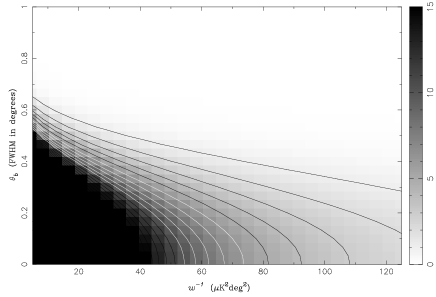
Figure 7: Contours $\Sigma=1,2,\ldots,10$ for an all-sky experiment. The noise $w^{-1}$ varies from $(5\mu K)^{2}(\rm{deg})^{2}$ to $(125\mu K)^{2}(\rm{deg})^{2}$. The no-noise axis (not plotted) is the 76.6 contour which asymptotically absorbs all other contours.

In the absence of noise ($w^{-1}=0$) one could in theory deconvolve a beam of any size without adding any extra uncertainty. It can be checked that in the all-sky case the $w^{-1}=0$ axis is the contour $\Sigma\approx 77$ of the detection function. This is also the maximum possible detection, imposed by cosmic variance, for an an all-sky single-dish experiment (with any beam). As soon as noise is taken into account, however, this upper limit is greatly reduced, and the beamsize becomes crucial. Even for the low (but realistic) level of noise $w^{-1}=(15\mu K)^{2}(\rm{deg})^{2}$ a modest 1-sigma detection requires $\theta_{b}=0.6^{\circ}$, whereas a 3-sigma detection requires $\theta_{b}=0.5^{\circ}$. This openly contradicts the naive argument favouring any beam with $\theta_{b}<0.85^{\circ}$. Although such beams do not start to cut off before $l=1000$, the noise is the real limiting factor. If the level of noise is pushed up to $w^{-1}=(125\mu K)^{2}(\rm{deg})^{2}$ an all sky experiment would never provide more than a 2-sigma detection, and even this would require $\theta_{b}=0.1^{\circ}$.

The all-sky diagram is misleading, however, as for some levels of noise and beam sizes it may be advantageous to reduce the sky coverage. In Fig. 8 we plot the detection function for $L=20$ degrees. We see that all combinations of noise and beamsize outside the $\Sigma=6$ contour for an all-sky experiment profit from reducing the sky coverage. We call this the noise-dominated region, and its complementary region signal-dominated.

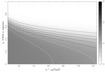
Figure 8: Same as Fig. 7, but for a square field with $L=20$ degrees.

The effects of noise are always reduced by concentrating all the observation time on a smaller area, since then we allow the same coherent signal to compete with the incoherent noise. It therefore makes sense that, if one is in the noise-dominated region, the detection function increases by reducing the area of sky observed. In the signal-dominated regions, on the other hand, the detection function is controlled by the cosmic/sample variance. Different observers in the Universe looking at different sky patches see different signals scattered about the theoretical average with a variance equal to the cosmic/sample variance. Although we cannot increase the number of skies observed, we can increase the area of sky sampled, thereby decreasing the cosmic/sample variance. For a given sample size the cosmic/sample variance limit is achieved at the no-noise axis and is roughly $\Sigma\approx 77L^{2}/(4\pi)$. By increasing $L$ the cosmic/sample variance decreases and so the detection function increases in signal-dominated regions.

The contrasting behaviour of the noise- and signal-dominated regions can be explained by the following semi-quantitative argument. From Eqn. (32) we have roughly

$$\Sigma^{2}\propto{\Omega^{s}\over{\left(1+{w^{-1}\Omega^{s}\over B_{i}^{2}C_{i}}\right)}^{2}}$$ (37)

where $C_{i}$ and $B_{i}$ are the average power spectrum and beam value for the bins used in estimating the convexity $\Sigma$. For a low signal-to-noise ratio, the noise term in the denominator dominates and so $\Sigma^{2}\propto 1/\Omega^{s}$. On the other hand, for a high signal-to-noise ratio, the noise term is much smaller than 1, and so $\Sigma^{2}\propto 1/\Omega^{s}-\beta\Omega^{s2}$, where $\beta\ll 1$.

The question naturally arises as to what is the ideal scanning strategy for a given experiment, and assuming that ideal strategy how significant is the detection of the sCDM secondary Doppler peaks. The answer to this question depends on the values of noise level $w^{-1}$, which itself depends on current detector technology and how effectively foreground emission can be subtracted. If we assume a low noise value (such as, for definiteness, $w^{-1}=(25\mu K)^{2}(\rm{deg})^{2}$), then the contours of $\Sigma$ in the beam-sky coverage plane are as shown in Fig. 9.

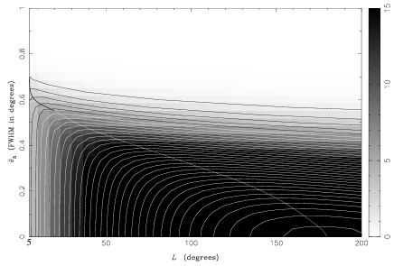
Figure 9: Low noise ($w^{-1}=(25\mu K)^{2}(\rm{deg})^{2}$) contours of the $\Sigma$ function. We allow the sky coverage $L$ to vary between 5 degrees and all sky ($L=202$ degrees), and consider beamsizes with FWHM between 0 and 1 degrees.

For any beamsize there is a maximum sky coverage beyond which the detection is not improved. If anything the level of the detection decreases, but typically not by much. The ideal scanning strategy is then defined by a line $L_{i}(\theta_{b})$ which intersects the contours of $\Sigma$ at the lowest $L$-value at which a plateau has been achieved in the detection function. The significance of the detection obtained for an ideally scanned experiment depends on the beam size. For example, if $\theta_{b}=0.6^{\circ}$, the ideal coverage is a patch of $L_{i}(0.6^{\circ})=5$ degrees, which results in a 3-sigma detection. If $\theta_{b}=0.5^{\circ}$, on the other hand, an 8-sigma detection can be obtained with $L_{i}=35$ degrees. The detection provided by an optimally scanned experiment increases at first very quickly as the beam is reduced below $\theta_{b}=0.6^{\circ}$ (from 3-sigma at $\theta=0.6^{\circ}$ to 33-sigma at $\theta_{b}=0.2^{\circ}$). By reducing $\theta_{b}$ from $0.2^{\circ}$ to zero, however, the detection is only increased by 2-sigma (from 33 to 35). For this level of noise the maximal detection is 35 sigma and is achieved with $\theta_{b}<3^{\prime}$ and all-sky coverage. For low noise levels all-sky coverage is never harmful, but it is the beamsize that determines how good a detection can be achieved, and how much sky coverage is actually required for an optimum level of detection.

For noise levels of the order $w^{-1}=(25\mu K)^{2}(^{o})^{2}$ the overall picture is always as in Fig. 9. In particular, there is always a top contour (like the $\Sigma=35$ contour in Fig. 9) referring to the maximal detection allowed by the given noise level. The maximum $\Sigma$ is always achieved with infinite resolution, but one falls short of this maximum by only a couple of sigmas if $\theta_{b}\approx 0.1^{\circ}$. If the noise is much smaller than this, however, the summit of $\Sigma$ is beyond $L=202^{\circ}$, as in Fig. 10. For $w^{-1}=(15\mu K)^{2}(\rm{deg})^{2}$, for instance, all-sky coverage becomes ideal for any $\theta_{b}<0.3^{\circ}$.

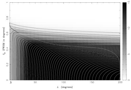
Figure 10: Very low noise ($w^{-1}=(15\mu K)^{2}(\rm{deg})^{2}$) contours of the $\Sigma$ function.

If, on the other hand, the noise is much larger than $w^{-1}=(25\mu K)^{2}(\rm{deg})^{2}$ then the $\Sigma$ contours are qualitatively different from Fig. 9. For, say $w^{-1}=(60\mu K)^{2}(\rm{deg})^{2}$, the contours of $\Sigma$ are shown in Fig. 11.

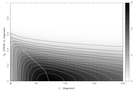
Figure 11: High noise ($w^{-1}=(60\mu K)^{2}(\rm{deg})^{2}$) contours of the $\Sigma$ function.

The beamsize is now a crucial factor. A beamsize of $\theta_{b}=0.5^{\circ}$ would provide a 3-sigma detection (with $L_{i}=10^{\circ}$), but reducing the beamsize to about $\theta_{b}=0.4^{\circ}$ improves the detection to 6-sigma (with $L_{i}=20^{\circ}$). Figure Fig. 11 also shows that, for high noise levels, forcing all-sky coverage dramatically decreases the detection.

We note finally that in interpreting the figures presented in this section, we must remember that in order to achieve low values of $w^{-1}$, the necessity for point source subtraction may severely limit the maximum possible sky coverage. In turn this can greatly reduce the significance of possible detections.

5.2 Interferometers

For inteferometer observations the detection function $\Sigma=\Sigma(w^{-1},\theta_{w},n_{\rm f})$, so it is a function of the noise level $w^{-1}$, the size of a single field (which is characterised by the FWHM of the Gaussian primary beam $\theta_{\rm w}\approx 2.35\sigma_{\rm w}$), and the number of such fields $n_{\rm f}$. Alternatively, noting that the solid-angle of a single field $\Omega_{\rm s}=\pi\sigma_{\rm w}^{2}$ we can instead write the detection function as $\Sigma=\Sigma(w^{-1},\theta_{w},\Omega_{\rm t})$, where $\Omega_{\rm t}=n_{\rm f}\Omega_{\rm s}$ is the solid angle of the total area of sky observed.

For ground-based interferometers it is expected that atmospheric effects will limit the shortest possible antenna spacing, which in turn will restrict the largest allowable FWHM of the primary beam to be $\sim$ 5 degrees. Since this is also close to the limit where convolution of the power spectrum becomes important for sCDM, in this section we shall restrict our attention to this case.

In Fig. 12 we have plotted the contours of $\Sigma$ for $\theta_{\rm w}=5^{\circ}$.

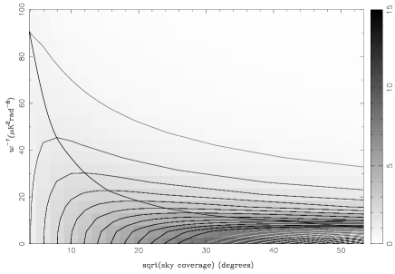
Figure 12: Contours of the detection function $\Sigma$ for an interferometer with a primary beam with $\theta_{w}=5^{\circ}$, for varying noise levels $w^{-1}$ and sky coverage.

As in the single-dish case, we we find that for any given noise level there is a sky coverage beyond which the detection function saturates and then starts to decrease. As the noise level decreases, the the saturation sky coverage increases along with the significance of the detection achieved.

In the high-noise régime $w^{-1}>(50\mu K)^{2}{\rm rad}^{-6}$ the ideal scanning strategy is to observe only a small sky area (a few fields at most), which results in only a 1- to 2-sigma detection. Increasing the sky coverage in the high-noise régime seriously decreases the level of the detection. We note that a 1-sigma dectection requires $w^{-1}<(100\mu K)^{2}{\rm rad}^{-6}$, and a 2 sigma detection may be achieved with $w^{-1}=(50\mu K)^{2}{\rm rad}^{-6}$. For $w^{-1}<(50\mu K)^{2}{\rm rad}^{-6}$ we enter the signal dominated region. By reducing $w^{-1}$ both the significance of the detection and the ideal sky coverage (no. of fields) increase very quickly. We note that observing just a single field provides only a 2-sigma detection dictated by cosmic/sample variance. By increasing the number of observed fields up to a saturation value, however, increases the level of the detection significantly. In the signal-dominated régime, increasing the number of fields beyond the ideal value decreases the detection only very slightly. For low noise levels $w^{-1}\approx(10\mu K)^{2}{\rm rad}^{-6}$ we see that an 9-sigma detection is possible for an ideal total sky coverage of $\Omega_{\rm t}\approx$ (45 deg)². We also note that in the low-noise case, detections of several sigma are possible even for relatively small sky-coverage. This is an important consideration if source subtraction is taken into account, since (as mentioned earlier) this severely limits the total possible sky coverage.

6 Distinguishing between cosmic strings and inflation

It is shown in Albrecht et al (1995) and Magueijo et al (1995) that the power spectrum of cosmic strings does not possess secondary Doppler peaks. It instead has a single peak at multipoles around $\ell=400-600$, although the height and precise shape of the peak are still subject to a considerable theoretical uncertainty.

If future observations of the CMBR show that the main peak in the true CMBR power spectrum is at lower multipoles, such as $\ell=200-250$ (as predicted by sCDM), then cosmic strings (in their present form) can be rejected as a possible theory for structure formation in the Universe. If, however, the main peak of the true CMBR power spectrum is shifted towards higher multipoles, then we must rely on the presence or absense of secondary peaks in order to distinguish between cosmic strings and CDM/inflation scenarios.

In this section we consider the case of maximal confusion by comparing a cosmic strings model and a CDM model for which the main peak in the power spectrum has the same position and shape (but the latter exhibits secondary peaks). For definiteness we have chosen a CDM theory with a flat primordial spectrum, $\Omega=0.3$, $h=0.6$, and $\Omega_{b}h^{2}=0.02$. We shall call this theory stCDM, the CDM competitor of cosmic strings. We have normalised the power spectra so that the height and shape of the main peak are similar in both cases. In principle we could now study the convexities associated with bins adjusted to the stCDM secondary oscillations, study the same quantities drawn from a cosmic strings spectrum, and then calculate the difference between the convexities average values in the two theories in units of the average variance. However, this procedure would define a ‘distance’ between the two theories which depends on the shape of the strings peak. We therefore simply study the first dip detection function of stCDM, and then take this detection function as a cosmic string rejection function.

In Fig. 13 we show the angular power spectrum of stCDM (solid line) and a possible power spectrum for cosmic strings (dotted line).

Figure 13: The angular power spectrum of stCDM (solid line) and one possible cosmic string scenario (dotted line). The dashed line is the stCDM power spectrum $C^{s}(k)$ as sampled by an interferometer with a primary of 2 degrees FWHM. The points indicate the average power in each bin for stCDM. The horizontal errorbars denote the width of the bins, and the vertical show the sample variance of the power estimtates for the same interferometer, assuming no noise.

We also plot the stCDM power spectrum $C^{s}(k)$ (divided by $\alpha$) as sampled by an interferometer with a primary beam of 2 degrees FWHM (dashed line). We see that, since the secondary peaks for stCDM are now much more separated in $\ell$ space (as compared to sCDM), the field size required for convolution of the power spectrum not to be a problem is much smaller. It can be checked that interferometers with a primary beam of FWHM $\ga 1.5$ degrees, and square windows (multiplied by a cosine bell) with $L\ga 4$ degrees are perfectly acceptable. We therefore assume these values as lower bounds on the field size for the purposes of cosmic string detection. For fields smaller than this deconvolution of the power spectrum would be necessary causing a deterioration of the detection function not taken into account in our calculations. However, we will see that the field must always be larger than this for any reasonable detection to be achieved, even baring deconvolution effects.

In Fig. 13 we also show the bins in $\ell$ chosen for the study of the convexity associated with the first dip in the stCDM power spectrum. The vertical errorbars are the sample variance errorbars associated with these bins for an interferometer with a primary beam of 2 degrees FWHM. We then repeat the same exercise as in the previous section concerning the detection function of the first dip of stCDM. In Figs. 14, 15, and 16, we redraw the experimental parameter space covered in Figs. 9, 11, and 12 but as applied to the first dip stCDM detection function. The only difference is that now we allow $L$ to start at 2 degrees. Similar, for interferometers, we consider a primary beam of 2 degrees FWHM. Again we make the point that if the effects of source subtraction are taken into account the total possible sky coverage may be severely limited, and this should be borne in mind when considering the figures presented in this section.

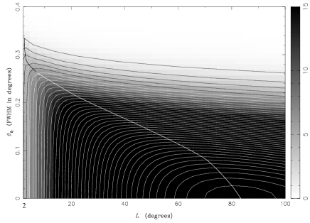
Figure 14: Low noise $w^{-1}=(25\mu K)^{2}(\rm{deg})^{2}$ contours of the detection function $\Sigma$ for stCDM.

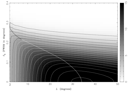
Figure 15: High noise $w^{-1}=(60\mu K)^{2}(\rm{deg})^{2}$ contours of the detection function $\Sigma$ for stCDM.

Overall we see that in signal dominated regions the detection is much better for stCDM than for sCDM. This is because features at higher $\ell$ have a smaller cosmic/sample variance (which is proportional to $1/\ell$). It can be checked that the cosmic/sample variance limit, obtained with a single-dish experiment with no noise, is now $\Sigma\approx 197L^{2}/(4\pi)$ (as opposed to $\Sigma\approx 77L^{2}/(4\pi)$ for sCDM). Even in the presence of noise, wherever the signal dominates, the detection is better for stCDM. However, in noise-dominated regions the behaviour of the detection function for stCDM and CDM is very different and the changes introduced follow a different logic for single-dish and interferometers.

For single-dish experiments the signal-dominated region is greatly reduced in stCDM. Much smaller beamsizes $\theta_{b}$ are now required for any meaningful detection. As shown in Figs. 14, and 15 one would now need $\theta_{b}<0.3^{\circ}$ and $\theta_{b}<0.25^{\circ}$, for noises $w^{-1}=(25\mu K)^{2}(\rm{deg})^{2}$ and $w^{-1}=(60\mu K)^{2}(\rm{deg})^{2}$ respectively, in order to obtain any reasonable detection. Again one can plot an ideal scanning line in the beam/coverage sections defined by a fixed noise $w^{-1}$. The ideal sky coverage is much smaller for stCDM than for sCDM. In general the countours of $\Sigma$ for stCDM compared to sCDM are squashed to lower $\theta_{b}$, lower $L$, and achieve higher significance levels, with steeper slopes. Following an ideal scanning line for any fixed $w^{-1}$ one reaches a maximal detection allowed by the given level of noise which is always better for stCDM than for sCDM. This maximal detection is normally obtained with a small sky coverage, and infinite resolution. Nevertheless, one falls short of this maximum by only a few sigma if the resolution is about $\theta_{\rm b}=4^{\prime}-6^{\prime}$. From Fig. 14, for $w^{-1}=(25\mu K)^{2}(\rm{deg})^{2}$, one may now obtain a maximal 43-sigma detection for an ideal scanning area of $L=65$ degrees. If $\theta_{b}=0.1^{\circ}$ a 36-sigma detection is still obtained. We also see that a beamsize of $\theta_{b}<0.25^{\circ}$ is required to obtain a 3-sigma detection (with $L=4$ degrees), and a 10-sigma detection can be achieved only with $\theta_{b}\approx 0.15^{\circ}$ (and $L_{i}=18$ degrees). All-sky coverage for an experiment targeting stCDM is generally inadvisable, and it would only be optimal for the unrealistically low levels of noise $w^{-1}<(11\mu K)^{2}(\rm{deg})^{2}$.

For interferometers the signal dominated regions are similar for sCDM and stCDM (compare Fig. 12 with Fig. 16).

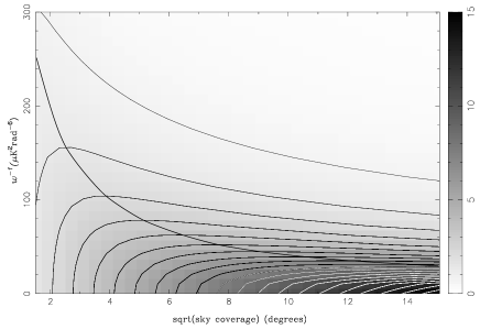
Figure 16: Contours of the detection function $\Sigma$ for stCDM for an interferometer with a primary beam with $\theta_{w}=2^{\circ}$, for varying noise levels $w^{-1}$ and sky coverage.

The borderline detection regions (where noise dominates), however, have expanded. This is because for stCDM we may make the primary beam smaller without running into convolution problems, which in turn reduces the instrumental noise. The high noise region is now $w^{-1}>(150\mu K)^{2}{\rm rad}^{-6}$. There one should observe only one or two $2^{\circ}$ fields, in order to obtain a detection between 1- and 2-sigma. For $w^{-1}<(150\mu K)^{2}{\rm rad}^{-6}$ we enter the signal dominated region. Following the ideal scanning line with decreasing $w^{-1}$, both the sky coverage and the level of the detection start increasing, at first first slowly, but then very quickly. Even for very high noise levels $w^{-1}=(100\mu K)^{2}{\rm rad}^{-6}$ one may obtain a 3-sigma detection with a total sky coverage of about (4 deg)² (which corresponds to only 7 independent fields) For relatively low-noise $w^{-1}=(20\mu K)^{2}{\rm rad}^{-6}$, on the other hand, we may obtain an 8-sigma detection with a sky coverage of around (10 deg)². Moreover, in the low-noise case, detections of several sigmas are possible for very small sky coverage.

7 Conclusions

We have studied the significance of secondary peak detection for sCDM and stCDM in a large parameter space of experiments, including interferometers and single-dish telescopes, and have adopted a broad minded attitude towards sky coverage. If point source subtraction is to be done in parallel with a CMBR experiment (so as to account for variable point-sources), however, a large sky-coverage may never be possible (see Section 4.3). This detail, often overlooked in satellite proposals, could then radically undermine a large number of estimates assisting experimental design. We will however not dwell on this awkward possibility, but while keeping it in mind, shall consider unrestricted sky coverage.

The results obtained are reported in Sections 5 and 6 and stress the contradictions of an all-purpose experiment. If the low-$l$ plateau of the spectrum is a theoretical target then one needs all-sky coverage, and satellite single-dish experiments are to be favoured. As shown in Section 5 even if one wishes to study Doppler peak features for sCDM all-sky coverage might still be preferable. Depending on the noise levels, a large sky coverage might be desirable, even for a resolution of about $\theta_{b}=0.4-0.5^{\circ}$.

Our work shows how such a design relies heavily on the assumption that the signal is in the vicinity of sCDM. If instead one is to test the high-$l$ opposition between low $\Omega$ CDM and cosmic strings, then we have seen that single-dish experiments are required to have rather high resolutions. Interferometers appear to be less constrained, providing 2-3 sigma detections under very unassuming conditions, with rapid improvements following further improvement in experimental conditions. Furthermore, in this context, all-sky scanning is not only unnecessary, but in fact undesirable. The best scanning is normally achieved with deep small patches. These two features contradict sharply the ideal experimental design motivated by the standard theoretical gospel.

Overall the parameter space of successful stCDM detections seems to increase for interferometers and shrink for single-dish when compared with sCDM. We believe that a variety of contrasting experimental techniques may equally well find their niche as regards important theoretical implications.

References

- [1] Albrecht A., Wandelt B., 1996, Phys.Rev.Lett., submitted
- [2] Albrecht A., Coulson D., Ferreira P., Magueijo J., 1996, Phys.Rev.Lett., 76, 1413
- [3] Becker R. H., White R. L., Helfand D. J., 1995, ApJ, 450, 559
- [4] Bond J. R., Efstathiou G., 1987, MNRAS, 226, 655
- [5] Crittenden R., Turok N., 1995, Phys. Rev. Lett., 75, 2642
- [6] Durrer R., Gangui A., Sakellariadou M., 1996, Phys. Rev. Lett., 76, 579
- [7] Gorski K. M., 1994, ApJ, 430, L85
- [8] Hobson M. P., Lasenby A. N., Jones M., 1995, MNRAS, 275, 863
- [9] Hu W., Sugiyama N., 1995a, ApJ, 444, 489
- [10] Hu W., Sugiyama N., 1995b, Phys. Rev. D, 51, 2599
- [11] Jungman G., Kamionkowski M., Kosowsky A., Spergel D., 1996, Phys. Rev. Lett., submitted
- [12] Kibble T. W. B., 1976, J. Phys., A9, 1387
- [13] Knox L., 1995, Phys. Rev. D, 52, 4307
- [14] Peebles J., 1973, ApJ, 185, 413
- [15] Steinhardt P., 1995, in Kolb E., Peccei R., eds, Proceedings of the Snowmass Workshop on Particle Astrophysics and Cosmology, Cosmology at the Crossroads. In press
- [16] Magueijo J., 1995, Phys.Rev. D, 52, 4361
- [17] Magueijo J., Albrecht A., Coulson D., Ferreira P., 1996, Phys.Rev.Lett., in press
- [18] Magueijo J., Hobson M. P., 1996, Phys.Rev.Lett., submitted
- [19] Press P. H., Teukolsky S. A., Vettering W. T., Flannery B. P., 1994, Numerical Recipes. Cambridge Univ. Press, Cambridge
- [20] Scott D., Srednicki M., White M., 1994, ApJ, 421, L5
- [21] Tegmark M., 1996, MNRAS, in press
- [22] Tegmark M., Efstathiou G., 1996, MNRAS, in press
- [23] Vilenkin A., Shellard P., 1994, Cosmic Strings and other Topological Defects. Cambridge Univ. Press, Cambridge
- [24] White M., Scott D., Silk J., 1994, A&AR, 32, 319