On Determining the Topology of the Observable Universe via 3-D Quasar Positions

Abstract

Hot big bang cosmology says nothing about the topology of the Universe. A topology-independent algorithm is presented which is complementary to that of Lehoucq et al.  1996 and which searches for evidence of multi-connectedness using catalogues of astrophysically observed objects. The basis of this algorithm is simply to search for a quintuplet of quasars (over a region of a few hundred comoving Mpc) which can be seen in two different parts of our past time cone, allowing for a translation, an arbitrary rotation and possibly a reflection. This algorithm is demonstrated by application to the distribution of quasars between redshifts of $z=1$ and $z\approx 4,$ i.e., at a comoving distance from the observer $1700h^{-1}\mbox{\rm Mpc}\,\lower 2.58334pt\hbox{$\buildrel<\over{\sim}$}\,d\,\lower 2.58334pt\hbox{$\buildrel<\over{\sim}$}\,3300h^{-1}\mbox{\rm Mpc}.$ Two pairs of isometric quintuplets separated by more than $300$$h^{-1}\mbox{\rm Mpc}$ are found. This is consistent with the number expected from Monte Carlo simulations in a simply connected Universe if the detailed anisotropy of sky coverage by the individual quasar surveys is taken into account. The linear transformation in (flat) comoving space from one quintuplet to another requires translations of $353$$h^{-1}\mbox{\rm Mpc}$ and 4922$h^{-1}\mbox{\rm Mpc}$ respectively, plus a reflection in the former case, and plus both a rotation and a reflection in the latter. Since reflections are required, if these two matches were due to multi-connectedness, then the Universe would be non-orientable.

1 Introduction

Given the immense observational effort to search for evidence of the possible non-trivial curvature of the observable Universe, (in particular for an “open”, i.e., negatively curved, $\Omega_{0}<1$, Universe) it is surely equally important to search for evidence for that the observable Universe could have a non-trivial topology. Apart from the obviously fundamental significance of knowing that the volume of the Universe is finite (if the topology turns out to be compact), studies of evolution of galaxies, quasars and other objects at cosmological distances would be immensely advanced by the ability to observe the same object at significantly different epochs. General relativity and the standard hot big bang model of the Universe are independent of topology. According to several authors (e.g., Hawking 1984; Zel’dovich & Grishchuk 1984), quantum gravity with a “no-boundary” boundary condition requires the Universe to be compact. A multi-connected topology of the observable Universe would provide such compactness.

Lachièze-Rey & Luminet (1995) present an extensive review of what multi-connectedness of our Universe would mean and of efforts made so far to detect multi-connectedness, so only a short introduction is given here.

A simple example of a 3-dimensional manifold with a non-trivial topology is the hypertorus. This can be constructed by identifying opposite faces of a cube (or more generally, a rectangular prism). A particle which one would otherwise expect to leave the cube at one surface “reenters” at the opposite face, without “noticing” that anything strange has happened. Many N-body simulations used to calculate the non-linear effects of gravity use a hypertoroidal topology in order to provide boundary conditions; this is termed using “periodic” boundary conditions. If the universe were hypertoroidal, then the identification of opposite faces would be physical, not merely a numerical technique.

A useful way of thinking about this in terms of a simply connected Universe is to imagine the cube repeated endlessly in a 3-dimensional grid. Each repetition consists of the same physical region of space, and photon paths (geodesics) can be calculated just as for the simply connected Universe. Our past time cone can then be thought of as before—but with the difference that we see the same chunk of the (whole) Universe at earlier and earlier epochs further and further away. This apparent space containing multiple copies of the Universe is called a “covering space”. In the case of the hypertorus, and if objects (e.g., quasars) had visible lifetimes as great as that of the Universe and were all bright enough to be seen in magnitude/surface-brightness limited surveys, then an obvious grid pattern would appear.

However, the hypertorus is only one of many possible topologies. There is an immense variety of topologies of the many possible 3-manifolds. For example, there are ten flat, homogeneous, isotropic, multi-connected 3-manifolds of finite volume (“compact”), and the classification of negatively curved, homogeneous, isotropic, multi-connected, compact 3-manifolds is still an open area of research (e.g., Thurston & Weeks 1984). Because of evolutionary effects and the vast range of possible topologies, the grid pattern possible for a hypertorus would not necessarily be obvious to the eye, so subjective impressions of present data are certainly not sufficient to rule out a non-trivial topology.

Other topologies can be thought of by starting with a “fundamental polyhedron” and identifying pairs of faces. Using the conventions of Lachièze-Rey & Luminet (1995), the shortest distance from an object to any of its “ghost” counterparts is labelled $\alpha$, and the largest distance from an object to an adjacent ghost (where there is an adjacent ghost for each face of the fundamental polyhedron) is labelled $\beta$. The choice of a fundamental polyhedron for thinking about a multi-connected topology is not unique; such a Universe (as considered here) is on average homogeneous and isotropic, without any borders in hypersurfaces of constant cosmological time.

The claimed periodicity of the galaxy redshift distribution in pencil-beam surveys (Broadhurst et al. 1990) could have been an indication of a non-trivial topology, but closer investigation of the data has not confirmed this. As argued thoroughly by Lachièze-Rey & Luminet (1995), observations on scales larger than this are not yet extensive enough to rule out repetitions of a finite-volume multiconnected Universe above a scale of about $\beta=600h^{-1}$ Mpc ($\alpha=300h^{-1}$ Mpc).

Figure 1: Example of “pseudo-structure” greater than the size of a compact Universe. The image is an Aitoff all-sky projection of a sphere of horizon radius ($6000h^{-1}$ Mpc) in the covering space; galactic latitudes smaller than 20^∘are excluded. The grey-scale indicates the value of $\delta T/T$ for each point on this sphere, where $\delta T/T$ is defined within the fundamental cube of size ($1000h^{-1}$ Mpc$)^{3}$ by $\delta T(x,y,z)/T(x,y,z)=\sin(2\pi x/1000h^{-1}\mbox{\rm\,Mpc}).$ The axes of the fundamental cube are arbitrarily rotated by $0{\cdot}5$ radians from the $l^{II}=0^{\circ}$ and $b^{II}=0^{\circ}$ axes. This all-sky map is not meant to be a realistic simulation of the CMB; it merely demonstrates that a small Universe containing a perturbation in $\delta T/T$ can appear to have structure in the covering space which is much larger than the size of the Universe itself. Note that these structures should not be confused with the circles predicted by Cornish et al. 1996 for a multi-connected Universe: in the latter case the circles are not (except in exceptional cases) of constant temperature.

Intuitively, one might think that a simple way to test for a compact topology would be to note that in a Universe of finite size no objects could exist which are larger than the size of the Universe, so that the initial perturbation spectrum (e.g., as observed by COBE) should be zero at large length scales, or small wavenumbers $k.$ The flaw in this argument is that in the covering space, structures which physically occupy the same, or nearly the same, part of space can coincide at the “faces” of the fundamental polyhedron in such a way that a pseudo-structure which is larger than the Universe can exist in the covering space. In analysis which works in the covering space (which is much easier than starting with a hypothesised topology), such a pseudo-structure would violate the minimum-$k$ criterion. As a demonstration, Fig. 1 shows a simple example of a sky map due to such pseudo-structure in a hypertoroidal Universe which is only a sixth of the horizon size. The huge structures which extend across the sky are simply due to the “microwave background” sphere cutting through the same (physical) structure at slightly different angles in adjacent ghost images of the fundamental polyhedron (cube).

While such a dramatic pattern should be easy to rule out, it is not clear what assumptions would be needed about the initial perturbation spectrum and the topology in order to make the minimum-$k$ test useful. In the example here, the maximum size of the fundamental polyhedron is clearly visible in the direction perpendicular to that of the pseudo-structures, so that averaging over the two dimensions of the sphere should help in the derivation of a generalised minimum-$k$ test. However, without a rigorous derivation of such a test, detailed models with assumptions about structure formation and specific topologies are required. Some authors have indeed calculated detailed models for particular cosmologies. In particular, toroidal topologies have been shown to be inconsistent with the COBE data to the scales of several thousand $h^{-1}$ Mpc (Stevens et al. 1993) to around the horizon size (Starobinsky 1993; de Oliveira & Smoot 1995) on the basis of considering a few (toroidal) of the topologies possible. Others (Jing & Fang 1994) note that the COBE data is well fit by a non-zero low wavelength cutoff in the primordial fluctuation spectrum, which would be consistent with a finite-volume, multiconnected Universe at about $1-3$ times the horizon scale.

An alternative to a minimum-$k$ test modified in some way by prior assumptions is the topology-independent method for searching for multi-connectedness in present and future CMB data which has been proposed by Cornish et al. (1996). This method is based on the property that a fundamental polyhedron of about the horizon size or smaller should intersect the last scattering sphere several times, in circles. Different copies of an intersection which represent the same subset of space-time should be seen in different parts of a CMB all-sky map. As long as the temperature of a point in the CMB is independent of the direction of the observer (e.g., the “Doppler” fraction of $\delta T/T$ due to the movement of the baryon-photon fluid towards or away from the observer is small), the values of $\delta T/T$ around corresponding circles should be identical apart from a rotation due to the particular multi-connected manifold explaining the identification. Note that the circles themselves are not of constant temperature: the pseudo-structures shown in Fig. 1 are not the same as the circles discussed by Cornish et al..

To put these tests into perspective, the reader is reminded that in comoving units, i.e., within the hypersurface of constant $t=t_{0},$ the distance to an object at redshift $z$ in the hypersurface of constant $t=t_{0}$ is $d=2(c/H_{0})(1-1/\sqrt{1+z}),$ the horizon is at $6000h^{-1}$ Mpc. (Except where otherwise stated, all distances here are quoted in comoving units.) The diameter across the observable Universe is, of course, twice the radius, i.e., $12000h^{-1}$ Mpc, so it could only be claimed that the observable Universe is simply connected if evidence were available up to a scale of twice the horizon size.

2 Method

Lehoucq et al.’s (1996) result that $\alpha\,\lower 2.58334pt\hbox{$\buildrel>\over{\sim}$}\,300h^{-1}$ Mpc was obtained from galaxy clusters using a very simple and powerful search method which avoids having to make prior assumptions on what the topology is. Their method consists of plotting a histogram of the apparent comoving separations between every pair of objects in a catalogue. If the catalogue samples a covering space containing several ghost images of the Universe, then the apparent separations of identical objects in the covering space would correspond to the sizes of various multiples and linear combinations of the translation vectors (between one copy of the Universe and the next). For every pair of copies of the Universe (containing $N$ objects of a certain class), there will $N(N-1)$ apparent separations of non-identical objects will be scattered around these “translation vector” values. Since the separations of identical objects are not scattered, sharp peaks in the histogram will appear at several of these favoured separations.

The most obvious candidates for detecting multi-connectedness on larger scales are quasars. However, applying Lehoucq et al.’s method to the quasar population would be weakened by evolutionary effects. Since quasar lifetimes are probably an order of magnitude or more less than the age of the Universe (e.g., Cavaliere & Padovani 1988), many of the pairs of quasars separated by the linear combinations of “translation vectors” will be observed at sufficiently different redshifts that they will only be bright enough to be visible at one of the two epochs. With the additional problem that the part of our past time cone systematically searched for quasars is still a small fraction of that available, the repetition effect necessary for obtaining sharp peaks is likely to be weak.

Therefore, I have chosen a more direct, (but slightly harder to program), algorithm which, as for Lehoucq et al.’s (1996) and Cornish et al.’s (1996) methods, does not assume any particular choice for the topology.

The idea is to search for a repetition in the universal covering space by searching for a quintuplet of several “close” quasars which exist in the same relative geometrical relation, modulo a rotation and/or a reflection, in at least two different parts of the observed universal covering space (i.e., in the hypersurface at constant cosmological time $t=t_{0}$ which corresponds to the interpretation of observations in ignorance of any possible multi-connectedness). The precise definition of “close” is that four of the quasars are each within $d_{c}\,\lower 2.58334pt\hbox{$\buildrel<\over{\sim}$}\,200h^{-1}$ Mpc of the fifth (arbitrarily chosen) quasar. Among the data set used (essentially that of quasars with $z>1$), containing $N=5114$ objects, the mean number of objects within this radius is $M=21.$ There are $\sim N(N-1)/2$ pairs of quasars. For each of the two quasars in a pair, there are $\sim M!/(M-4)!$ quintuplets which can be formed with four “close” companions. A naïve implementation of this technique would therefore require $\sim N(N-1)/2\;[M!/(M-4)!]^{2}\sim N^{2}M^{8}\,\lower 2.58334pt\hbox{$\buildrel<\over{\sim}$}\,10^{18}$ comparisons of geometry between quintuplets, way beyond present computing capabilities.

This number of operations can be reduced drastically by using subsets of the geometrical criteria to filter out impossible cases at appropriate stages of the algorithm, therefore wasting no more operations on such cases. The algorithm is as follows.

For a given pair of quasars, a list of the “close” companions (hereafter “secondaries”) of each is made. The distance of each secondary from its primary is calculated. The lists of primary-secondary distances for the two primaries are searched for identical values. In the case of genuinely matching quintuplets (where the primaries correspond in this match), the four primary-secondary distances around each primary are identical, so should pass this first filter. Hereafter, this filtering process is termed “distance matching”. This ends up with a list of zero, four or more candidate secondaries for each primary.

For each list of remaining candidate secondaries, the angle formed by each pair of candidates with its primary quasar is calculated, making two lists of companion-primary-companion angles. These two lists of companion-primary-companion angles are then searched for identical values (between the two lists). Hereafter, this is referred to as “angle matching”. Once again, if there is a genuine quintuplet match, this will create six companion-primary-companion angles which match. These two filters, “distance matching” and “angle matching”, drastically reduce the number of secondaries remaining in the list of “candidate” secondaries, making the problem computable in practice.

Still considering the same pair of primary quasars, a search is then made for four secondaries among which each of the six possible secondary-primary-secondary angles has corresponding matches around the second primary quasar. This guarantees that the two quintuplets (each composed of primary plus four secondaries) are isometric within the tolerances chosen.

The choice of quintuplets rather than, say, quadruplets or sextuplets, is a compromise based on the data and computing power available. The probability of finding corresponding $n$-tuplets which are simply due to chance is larger for smaller $n,$ while the number of computing operations required is larger for larger $n.$

The main astrophysical uncertainties which could affect this method (apart from the problem of the physics of quasar lifetimes!) are those in the comoving radial distances. These are due to (1) the uncertainty in the spectroscopic measurement of the redshift and (2) the peculiar velocity of the quasar relative to the comoving reference frame. The latter causes (2a) a movement relative to the comoving reference frame between the two redshifts at which the quasar is observed and (2b) a misestimate of the quasar’s comoving radial distance due to inclusion of the peculiar velocity doppler shift as part of the cosmological redshift.

The most serious of these constraints is (2b): a quasar at $z=2$ having a peculiar radial velocity of $v_{pec}=400\mbox{\rm km s}^{-1}$ has its comoving radial distance misestimated by about $5h^{-1}$ Mpc. The “movement” error (2a) is likely to be less than about $0{\cdot}5h^{-1}$ Mpc (for $v_{pec}=400\mbox{\rm km s}^{-1}$ and observations of the two images at $z=1$ and $z=3$ the error is $0{\cdot}6h^{-1}$ Mpc), while the measurement error (1) lies at either of these two values depending on the whether the redshifts are available to $\delta(z)=0{\cdot}01$ or $\delta(z)=0{\cdot}001$ respectively. (These estimates assume $\Omega_{0}=1,\lambda_{0}=0$.)

3 Results

This algorithm was applied to a catalogue of $N=5114$ objects (nearly all quasars, but including a few galaxies) with redshifts greater than unity found in the NASA/IPAC Extragalactic Database (NED, primarily from surveys by Hewitt & Burbidge (1989), Crampton et al. (1988), Boyle et al. (1990) and Schneider et al. (1992)).

The distance defining “close” used was $d_{c}=$ $200h^{-1}$ Mpc, the tolerance for primary-secondary distances to be considered identical was $\Delta d=0.5$$h^{-1}\mbox{\rm Mpc}$ or $\Delta d=1$$h^{-1}\mbox{\rm Mpc}$, and the tolerance for secondary-primary-secondary angles to be considered identical was $\Delta\theta=0{\cdot}01$ rad. The algorithm takes about $10^{1}$ hours to run on a Sun Sparcstation 10.

Early attempts (using the $N=4848$ quasars available from NED in Oct 1994, and $\Delta d=0.5$$h^{-1}\mbox{\rm Mpc}$) resulted in 56 pairs of such quintuplets found in the data. Intuitively, it seems extraordinary that these matches could be due to chance. However, a random data set was simulated, containing the same number of objects as in the quasar list and distributed according to the same density distribution. As the density distribution is not very uniform, combining a variety of different observational selection criteria, this was done by retaining the celestial positions of all the objects in the observed data, but reassigning the observed redshifts randomly to obtain a 3-dimensional random catalogue. This process should destroy any real matching quintuplets in the data. The results over several (8) simulations were $57\pm 10$ ($1-\sigma$ uncertainty) pairs of matching quintuplets. So, if there are any real pairs of matching quasar quintuplets due to multi-connectedness, these are swamped by coincidences simply due to Poisson statistics.

One way of trying to avoid the random coincidences was by introducing an independent criterion, the result of Lehoucq et al. (1996): the “minimum” size of the fundamental polyhedron (if it exists) must be greater than $\alpha=300$$h^{-1}\mbox{\rm Mpc}$.

Applying this requirement that the separation between the quintuplets is greater than $\alpha=300$$h^{-1}\mbox{\rm Mpc}$ (using the full $N=5114$ quasar catalogue and $\Delta d=1$$h^{-1}\mbox{\rm Mpc}$), 2 pairs of matching quintuplets were found in the data, while only $0{\cdot}54\pm 0{\cdot}66$ were found in simulations (performed as before) based on this data. Table 1 lists positions (right ascension and declination, equinox B1950.0, and redshift) for the matching quintuplets. In Figures 1 and 2, the objects near a quintuplet are shown linearly transformed to the position of the “ghost” quintuplet. The transformations require translations of 353$h^{-1}\mbox{\rm Mpc}$ and 4922$h^{-1}\mbox{\rm Mpc}$ respectively, plus a reflection in the former case, and both a rotation and a reflection in the latter case. Since reflections are involved in both transformations, if the matches were due to multi-connectedness, then the Universe would be non-orientable.

Table 1: Positions of the pairs of isometric quasar quintuplets

$$\begin{array}[]{l c c c@{\ \ \ }l c c c}\lx@intercol\hfil{\rm Object}\hfil\lx@intercol&\lx@intercol\hfil{}\alpha{}\hfil\lx@intercol&\lx@intercol\hfil{}\delta{}\hfil\lx@intercol&\lx@intercol\hfil z\hfil\lx@intercol&\lx@intercol\hfil{\rm Object}\hfil\lx@intercol&\lx@intercol\hfil{}\alpha{}\hfil\lx@intercol&\lx@intercol\hfil{}\delta{}\hfil\lx@intercol&\lx@intercol\hfil z\hfil\lx@intercol\\ \hline\cr\lx@intercol\hfil{\rm First\ Quintuplet\ Pair}\hfil\lx@intercol\\ \hline\cr{\rm[HB89]\ 0122-334}&1{}^{h}{}22{}^{m}{}37.9{}^{s}{}&-33{}^{\circ}{}25{}{{}^{\prime}}{}43{}{{}^{\prime\prime}{}}&2.260&{\rm[HB89]\ 0103-271}&1{}^{h}{}03{}^{m}{}07.8{}^{s}{}&-27{}^{\circ}{}07{}{{}^{\prime}}{}37{}{{}^{\prime\prime}{}}&2.180\\ {\rm[HB89]\ 0114-358}&1{}^{h}{}14{}^{m}{}13.2{}^{s}{}&-35{}^{\circ}{}52{}{{}^{\prime}}{}42{}{{}^{\prime\prime}{}}&2.260&{\rm[HB89]\ 0050-280}&0{}^{h}{}50{}^{m}{}05.8{}^{s}{}&-28{}^{\circ}{}04{}{{}^{\prime}}{}24{}{{}^{\prime\prime}{}}&2.152\\ {\rm[HB89]\ 0123-368}&1{}^{h}{}23{}^{m}{}38.8{}^{s}{}&-36{}^{\circ}{}48{}{{}^{\prime}}{}12{}{{}^{\prime\prime}{}}&2.205&{\rm[HB89]\ 0049-261}&0{}^{h}{}49{}^{m}{}30.1{}^{s}{}&-26{}^{\circ}{}06{}{{}^{\prime}}{}48{}{{}^{\prime\prime}{}}&2.060\\ {\rm[HB89]\ 0109-355}&1{}^{h}{}09{}^{m}{}07.5{}^{s}{}&-35{}^{\circ}{}31{}{{}^{\prime}}{}23{}{{}^{\prime\prime}{}}&2.307&{\rm[HB89]\ 0049-290}&0{}^{h}{}49{}^{m}{}29.8{}^{s}{}&-29{}^{\circ}{}00{}{{}^{\prime}}{}41{}{{}^{\prime\prime}{}}&2.220\\ {\rm[HB89]\ 0113-327\ NED02}&1{}^{h}{}13{}^{m}{}30.8{}^{s}{}&-32{}^{\circ}{}46{}{{}^{\prime}}{}23{}{{}^{\prime\prime}{}}&2.260&{\rm[HB89]\ 0103-290}&1{}^{h}{}03{}^{m}{}02.7{}^{s}{}&-29{}^{\circ}{}05{}{{}^{\prime}}{}53{}{{}^{\prime\prime}{}}&2.230\\ \hline\cr\lx@intercol\hfil{\rm Second\ Quintuplet\ Pair}\hfil\lx@intercol\\ \hline\cr{\rm[CCS88]\ 133918.2+271659}&13{}^{h}{}39{}^{m}{}18.2{}^{s}{}&27{}^{\circ}{}16{}{{}^{\prime}}{}59{}{{}^{\prime\prime}{}}&1.754&{\rm[HB89]\ 0104-381\ NED02}&1{}^{h}{}04{}^{m}{}56.2{}^{s}{}&-38{}^{\circ}{}07{}{{}^{\prime}}{}07{}{{}^{\prime\prime}{}}&2.060\\ {\rm[HB89]\ 1339+280}&13{}^{h}{}39{}^{m}{}22.8{}^{s}{}&28{}^{\circ}{}02{}{{}^{\prime}}{}04{}{{}^{\prime\prime}{}}&1.965&{\rm[HB89]\ 0117-374}&1{}^{h}{}17{}^{m}{}40.4{}^{s}{}&-37{}^{\circ}{}25{}{{}^{\prime}}{}29{}{{}^{\prime\prime}{}}&1.940\\ {\rm[HB89]\ 1343+266\ NED01}&13{}^{h}{}43{}^{m}{}24.7{}^{s}{}&26{}^{\circ}{}40{}{{}^{\prime}}{}06{}{{}^{\prime\prime}{}}&2.030&{\rm[HB89]\ 0114-368}&1{}^{h}{}14{}^{m}{}44.8{}^{s}{}&-36{}^{\circ}{}52{}{{}^{\prime}}{}21{}{{}^{\prime\prime}{}}&1.820\\ {\rm[CCS88]\ 133211.4+280201}&13{}^{h}{}32{}^{m}{}11.4{}^{s}{}&28{}^{\circ}{}02{}{{}^{\prime}}{}01{}{{}^{\prime\prime}{}}&1.706&{\rm[HB89]\ 0106-379}&1{}^{h}{}06{}^{m}{}54.7{}^{s}{}&-37{}^{\circ}{}56{}{{}^{\prime}}{}18{}{{}^{\prime\prime}{}}&2.200\\ {\rm[CCS88]\ 133243.2+272958}&13{}^{h}{}32{}^{m}{}43.2{}^{s}{}&27{}^{\circ}{}29{}{{}^{\prime}}{}58{}{{}^{\prime\prime}{}}&1.515&{\rm[HB89]\ 0055-387}&0{}^{h}{}55{}^{m}{}01.8{}^{s}{}&-38{}^{\circ}{}44{}{{}^{\prime}}{}44{}{{}^{\prime\prime}{}}&2.350\\ \hline\cr\end{array}$$

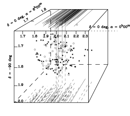
Figure 2: Superposition of quasars within 200$h^{-1}\mbox{\rm Mpc}$ of [HB] 0122-334 with the quasars within 200$h^{-1}\mbox{\rm Mpc}$ of [HB89] 0103-271, using the linear transformation mentioned in the text. (All distances mentioned here are comoving.) The axes are parallel to the directions in right ascension and declination as labelled, units are in redshift. Unshifted quasars are shown as stars, shifted quasars are shown as open circles. For clarity, vertical lines are omitted except for the members of the matching quintuplets.

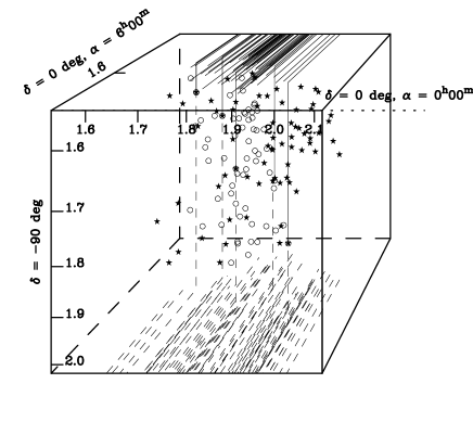
Figure 3: Superposition of quasars within 200$h^{-1}\mbox{\rm Mpc}$ of [CCS88] 133918.2+2716 with the quasars within 200$h^{-1}\mbox{\rm Mpc}$ of [HB89] 0104-381 NED02, using the linear transformation mentioned in the text. Axes and symbols are as for Fig. 1.

However, a more conventional explanation (within a simply-connected Universe) is available by noting that the Monte Carlo simulations could lose some clustering properties existent in the observational quasar distribution. Regions in which the (observed) quasar number density is higher have more objects, and therefore more chance correspondences. Three of the twenty individual members of the matching quintuplets are in fact binaries (indicated by “NED01” or “NED02” in Table 1), though this may not have any relation to clustering. The underlying astrophyical clustering of quasars (after correction for selection effects) seems to follow galaxy clustering with a clustering length of around 6-10$h^{-1}\mbox{\rm Mpc}$ (Andreana & Cristiani 1992), and so there should be little clustering at the scales of the quintuplets: separations between individual members of a quintuplet range from 57$h^{-1}\mbox{\rm Mpc}$  to 353$h^{-1}\mbox{\rm Mpc}$, with a median separation of 152$h^{-1}\mbox{\rm Mpc}$.

Instead, an explanation lies at the level of “observational” clustering. The quasar sample is composed of a large number of individual surveys. In the creation of the random simulations, the redistribution of the redshifts of the entire catalogue therefore gives the same average redshift distribution to each of the individual surveys. This average redshift distribution may be sufficiently different from the original redshift distribution in a survey to affect the number of chance coincidences. The full catalogue was therefore divided up into 93 individual “surveys” over small solid angles such that the redshift distributions in individual catalogues were isotropic within each “surveyed” region; the remaining 1751 quasars spread across the sky were considered as a single “survey”. Random simulations were then performed by redistributing the redshifts within the individual “surveys”, again retaining the observed set of positions on the sky. The result over 15 simulations was $1{\cdot}1\pm 1{\cdot}2$ isometric quintuplet pairs, so the detection of 2 quintuplet pairs in the data is not at all statistically significant. It serves instead as an illustration of what a positive detection could be like.

4 Conclusion

A topology-independent method, complementary to those of Lehoucq et al. 1996 and Cornish et al. 1996, which observationally searches for the effects of a non-trivial topology of the observable Universe has been presented. The method is simply to search for isometries of quasar quintuplets in different parts of our past time cone, and an algorithm which reduces the number of computations required to within practical computing cabilities has been explained.

This method is illustrated by application to the observed set of quasars available from NED, and the significance is tested by comparison to Monte Carlo simulations. Even by taking advantage of Lehoucq et al.’s (1996) (and others’) results against the Universe having a multi-connected topology on a scale $\alpha\leq 300$$h^{-1}\mbox{\rm Mpc}$, the number of detections remains statistically consistent with that expected for a simply connected Universe.

Without a detailed physical model of quasar evolution, the method is only capable of finding evidence for multi-connectedness, not for showing simple-connectedness. If a statistically significant number of corresponding quintuplets were found in a future more complete catalogue of quasars, it should be followed by finding a fundamental polyhedron and linear transformations which explain the quintuplet matches found. These should be applied to the full quasar catalogue in order to find the transformed (“ghost”) quasar positions in the copy of the fundamental polyhedron in which galaxy and galaxy cluster positions are best known, i.e., in the region of the covering space containing the Galaxy. If the transformed positions of the quasars significantly corresponded to the centres of, say, bright elliptical galaxies, or cluster centres, this would be a confirmation of multi-connectedness, and an indication of the evolutionary link between quasars and galaxies. On the contrary, a limit on the absence of luminous objects at the transformed quasar positions would either be a refutation of the claimed multi-connected manifold or evidence that the luminosity of “dead” quasars falls below the detection limit.

5 acknowledgements

Thanks to Andrew Liddle, John Barrow and Amr El-Zant of the University of Sussex Astronomy Centre for useful suggestions and comments. This research has been carried out with support from the Institut d’Astrophysique de Paris, CNRS, from a PPARC Research Fellowship and has made use of Starlink computing resources and the NASA/IPAC extragalactic database (NED) which is operated by the Jet Propulsion Laboratory, Caltech, under contract with the National Aeronautics and Space Administration.

References

- [1]
- [2] Boyle, B. J., Fong, R., Shanks, T., And Peterson, B. A. (1990), MNRAS, 243, 1
- [3]
- [4] Broadhurst, T.J., Ellis, R.S., Koo, D.C. & Szalay, A.S., 1990, Nature, 343, 726
- [5]
- [6] Cavaliere, A. & Padovani, P, 1988, ApJ, 333, L33
- [7]
- [8] Cornish, N.J., Spergel, D.N. & Starkman, G.D., SISSA, preprints, gr-qc/9602039
- [9]
- [10] Crampton, D., Cowley, A. P., Schmidtke, P. C., Janson, T. & Durrell, P., 1988, AJ, 96, 816
- [11]
- [12] de Oliveira Costa, A. & Smoot, G.F., 1995, ApJ, 448, 477
- [13]
- [14] Hawking, S., 1984, NuclPhysB, 239, 257
- [15]
- [16] Hewitt, A., Burbidge, G., A New Optical Catalog Of Quasi-Stellar Objects, magnetic tape 1989
- [17]
- [18] Jing, Y.-P. & Fang, L.-Z., 1994, SISSA, preprints, astro-ph/9409072
- [19]
- [20] Lachièze-Rey, M. & Luminet, J.-P., 1995, PhysRep, 254, 136
- [21] Lehoucq, R., Luminet, J.-P. & Lachièze-Rey, M., 1996, preprint
- [22]
- [23] Schneider, D. P., Bahcall, J. N., Saxe, D. H., Bahcall, N. A., Doxsey, R., Golombeck, D., Krist, J., Mcmaster, M., et al., 1992, PASP, 104, 678
- [24]
- [25] Starobinsky, A.A., 1993, JETPLett, 57, 622
- [26]
- [27] Stevens, D., Scott, D. & Silk, J., 1993, PhysRevLett, 71, 20
- [28]
- [29] Thurston, W.P. & Weeks, J.R., 1984, ScAmer, July, 94
- [30]
- [31] Zel’dovich, Y.B. & Grishchuk, L.P., 1984, MNRAS, 207, 23P