High-Order Correlations of Peaks and Halos:
a Step toward Understanding Galaxy Biasing

Abstract

We develop an analytic model for the hierarchical correlation amplitudes $S_{j,g}(R)\equiv{\overline{\xi}}_{j,g}(R)/{\overline{\xi}}_{2,g}^{j-1}(R)$ [where $j=3$,4,5, and ${\overline{\xi}}_{j,g}(R)$ is the $j$th order connected moment of counts in spheres of radius $R$] of density peaks and dark matter halos in the quasi-linear regime. The statistical distributions of density peaks and dark matter halos within the initial density field (assumed Gaussian) are determined by the peak formalism of Bardeen et al. (1986) and by an extension of the Press-Schechter formalism, respectively. Modifications of these distributions caused by gravitationally induced motions are treated using a spherical collapse model. We test our model against results for $S_{3,g}(R)$ and $S_{4,g}(R)$ from a variety of N-body simulations. The model works well for peaks even on scales where the second moment of mass (${\overline{\xi}}_{2}$) is significantly greater than unity. The model also works successfully for halos that are identified earlier than the time when the moments are calculated. Because halos are spatially exclusive at the time of their identification, our model is only qualitatively correct for halos identified at the same time as the moments are calculated. For currently popular initial density spectra, the values of $S_{j,g}$ at $R\sim 10\,h^{-1}{\rm{Mpc}}$ are significantly smaller for both halos and peaks than those for the mass, unless the linear bias parameter $b$ [defined by $b^{2}={\overline{\xi}}_{2,g}(R)/{\overline{\xi}}_{2}(R)$ for large $R$] is comparable to or less than unity. The $S_{j,g}$ depend only weakly on $b$ for large $b$ but increase rapidly with decreasing $b$ at $b\sim 1$. Thus if galaxies are associated with peaks in the initial density field, or with dark halos formed at high redshifts, a measurement of $S_{j,g}$ in the quasi-linear regime should determine whether galaxies are significantly biased relative to the mass. We use our model to interpret the observed high order correlation functions of galaxies and clusters. We find that if the values of $S_{j,g}$ for galaxies are as high as those given by the APM survey, then APM galaxies should not be significantly biased.

1 INTRODUCTION

A fundamental problem in cosmology is to understand how the spatial distribution of galaxies (and of galaxy clusters) is related to that of the underlying mass. In standard models of galaxy formation, it is assumed that galaxies form by the cooling and condensation of gas within dark matter halos (White & Rees 1978; White & Frenk 1991). Nongravitational processes which cannot be modeled reliably are likely to be critical in determining the properties of individual galaxies, yet they should have little effect on the formation and clustering of dark halos. As a result, the problem of galaxy biasing can be approached by first understanding how dark halos are distributed relative to the mass.

Dark halos are highly nonlinear objects and their formation and clustering has usually been studied using N-body simulations (e.g. Frenk 1991; Gelb & Bertschinger 1994 and references therein). Such simulations are limited both in resolution and in dynamical range and can be difficult to interpret. Our understanding of their results could be substantially enhanced by simple physical models and the analytic approximations they provide. Mo & White (1996) have developed a model for the second order correlation functions of dark halos based on the Press-Schechter formalism (Press & Schechter 1974; hereafter PS). Here we extend their work to derive a model for the higher order correlations. We also work out a similar model for peaks in the initial density field.

In the PS formalism, one defines dark matter halos at any given time as regions of the initial density field which just collapse at that time according to a spherical infall model. This formalism can be extended so that it predicts not only the mass function of dark halos, but also a wide range of other statistical properties of the hierarchical clustering process; comparisons with N-body simulation data show detailed agreement (e.g. Bond et al. 1991; Bower 1991; Kauffmann & White 1993; and particularly, Lacey & Cole, 1993, 1994). Mo & White (1996) showed that the PS formalism and its extensions can be used to construct a model for the spatial correlation of dark halos in hierarchical models. They used the standard PS formalism both to define dark halos from the initial density field, and to specify how their mean abundance within a large spherical region is modulated by the linear mass overdensity in that region. The gravitationally induced evolution of clustering was treated by assuming that each region evolves as if spherically symmetric. The model was found to give an accurate description of the bias function, $b_{h}(R,\delta)={\delta_{h}}(R,\delta)/\delta$, where ${\delta_{h}}(R,\delta)$ is the mean overdensity of halos within spheres which have radius $R$ and mass overdensity $\delta$. A simple extension provides a surprisingly accurate prediction for the halo-halo two-point correlation measured in N-body simulations (Mo & White 1996; Mo, Jing & White 1996). It is clearly interesting to see if such a model can also be constructed for the higher order correlations of dark halos.

In the peak formalism, one assumes that galaxies form at those peaks of a suitably smoothed version of the initial density field which rise above some density threshold. Kaiser (1984) introduced this idea to show how the strong clustering of Abell clusters could result from the statistics of high peaks in a Gaussian initial field. This formalism was later developed extensively by Bardeen et al. (1986, hereafter BBKS). These authors showed that if galaxies can be associated with high peaks of the initial density field then they should be more strongly clustered than the mass, an effect usually called “galaxy biasing”. Unfortunately it is not known how well galaxies correspond to high peaks of the initial field, and it is unclear how to deal with the problem that the present-day clustering of peaks differs substantially from that in the initial (Lagrangian) space because of gravitationally induced motions. As a result, the predictions of the theory have only been checked quantitatively by direct N-body simulation of the motion of the material associated with density peaks (e.g. Davis et al. 1985; Frenk et al. 1988; Katz, Quinn & Gelb 1993). In this paper we will show that the idea underlying the model of Mo & White can also be used to construct a model for the correlation functions of peaks in physical space. We use the theory of Bardeen et al. to define peaks from the initial density field, and to specify how their mean abundance within a large spherical region is modulated by the linear mass overdensity in that region. The gravitationally induced evolution of clustering is then treated, as in the model of Mo & White, by assuming that each region evolves according to a spherical collapse model.

We describe our model in §2, and present detailed tests of its predictions against N-body simulations in §3. Then in §4 we demonstrate how it can be used to interpret the observed high order correlation functions of galaxies and of clusters of galaxies, and to determine whether or not galaxies are biased relative to mass. Finally, in §5 we summarize our main results.

2 THE MODEL

To calculate the high order moments of peaks and halos (together called “galaxies”), we use the general formalism developed by Fry & Gaztanaga (1993). Consider the present-day mass overdensity field $\delta({\bf{x}})=[\rho({\bf{x}})-\overline{\rho}]/\overline{\rho}$, where $\rho({\bf{x}})$ is the local mass density and $\overline{\rho}$ the mean density. When smoothed in spherical window $W(x;R)$ with characteristic radius $R$, $\delta({\bf{x}})$ gives rise to a smoothed density field:

$$\delta({\bf{x}};R)=\int W(|{\bf{x}}-{\bf{y}}|;R)\delta({{\bf{y}}})d^{3}y.$$

For a top-hat window, $\delta({\bf{x}};R)$ is just the volume average of $\delta({\bf{x}})$ within a sphere of radius $R$. The statistical properties of $\delta({\bf{x}};R)$ are described by the one-point distribution function of the density field. Now let us denote the overabundance of “galaxies” in the same window by ${\delta_{{g}}}({\bf{x}};R)$. If ${\delta_{{g}}}({\bf{x}};R)$ is completely determined by $\delta({\bf{x}};R)$, then we can write ${\delta_{{g}}}$ as a function of $\delta$, ${\delta_{{g}}}=F(\delta)$, which should not depend on ${\bf{x}}$. (Note that this can hold at best approximately; see below.) To simplify notation, we will omit writing explicitly the smoothing radius $R$ associated with $\delta$ and ${\delta_{{g}}}$. In general, we can expand $F$ in Taylor series:

$${\delta_{{g}}}=F(\delta)=\sum_{k=0}^{\infty}{b_{k}\over k!}\delta^{k},$$

where $b_{k}$ are constant. Fry & Gaztanaga (1993) have shown that if the volume averaged j-point mass correlation functions ${\overline{\xi}}_{j}(R)$ have the hierarchical form:

$${\overline{\xi}}_{j}(R)=S_{j}{\overline{\xi}}_{2}^{j-1}(R),$$

then the transformation given by equation (2) preserves the hierarchical structure in the limit ${\overline{\xi}}_{2}(R)\ll 1$. In this case one can write

$${\overline{\xi}}_{{{j}},g}(R)=S_{{{j}},g}{\overline{\xi}}_{g,2}^{j-1}(R),$$

and for $j=3$, 4 and 5, which are relevant for our later discussion, one has

$$S_{3,g}=b^{-1}(S_{3}+3c_{2}),$$

$$S_{4,g}=b^{-2}(S_{4}+12c_{2}S_{3}+4c_{3}+12c_{2}^{2}),$$

$$S_{5,g}=b^{-3}\left[S_{5}+20c_{2}S_{4}+15c_{2}S_{3}^{2}+(30c_{3}+120c_{2}^{2})S_{3}+5c_{4}+60c_{3}c_{2}+60c_{2}^{3}\right],$$

where $c_{k}=b_{k}/b$ and $b=b_{1}$. Thus to obtain the high order moments $S_{{{j}},g}$ for halos and peaks in the quasilinear regime, we need to work out the coefficients $b_{k}$ in the bias relation (equation 2). We will do this in §2.2 and §2.3.

It is important to emphasize that the bias relation given by equation (2) is at best approximate. This is because ${\delta_{{g}}}$ in a spherical region with mean mass overdensity $\delta$ must depend not only on $\delta$ but also on the internal structure of the region and on the external tides acting on it. As a result, there must be scatter in the “galaxy” counts among spheres with the same $\delta$ and $R$. Such scatter should also contribute to the high order moments. As discussed in Mo & White (1996), this contribution must be important on scales which are not much larger than the linear Lagrangian sizes of the “galaxies”. On larger scales it may or may not be important, and since it cannot be estimated within our formalism, in the present paper we will assume it to be negligible and test the resulting predictions against N-body data.

2.1 Initial density field

The initial overdensity field $\delta({\bf{x}})\equiv[\rho({\bf{x}})-{\bar{\rho}}]/{\bar{\rho}}$ is assumed to be Gaussian and so to be described by a power spectrum $P(k)\delta_{D}({\bf{k}}-{\bf{k}}_{1})=\langle\delta({\bf{k}})\delta({\bf{k}}_{1})\rangle$, where $\delta({\bf{k}})$ is the Fourier transform of $\delta({\bf{x}})$ and $\delta_{D}({\bf{k}})$ is the Dirac delta function. We smooth the field $\delta({\bf{x}})$ by convolving it with a spherically symmetric window function $W(x;R)$ having comoving characteristic radius $R$ (measured in current units). The smoothed field can be written as

$$\delta({\bf{x}};R)=\int{\hat{W}}(k;R)\delta_{{\bf{k}}}\exp(i{{\bf{k}}}\cdot{\bf{x}})d^{3}k,$$

where ${\hat{W}}(k;R)$ is the Fourier transform of the window function $W(x;R)$. Following BBKS, we define the order $l$ moment of the smoothed field by

$$\sigma_{l}^{2}(R)=\int{\hat{W}}^{2}(k;R)P(k)k^{2l}d^{3}k.$$

The order zero moment, which we denote by $\Delta^{2}(R)$, is just the rms fluctuation of mass in the smoothing window.

For a given window function the smoothed field $\delta({\bf{x}};R)$ is Gaussian and so has the following one-point distribution function

$$p(\delta;R)d\delta={1\over(2\pi)^{1/2}}\exp\left[-{\delta^{2}\over 2\Delta^{2}(R)}\right]{d\delta\over\Delta(R)}.$$

Since both $\delta$ and $\Delta(R)$ grow with time in the same manner in linear perturbation theory, it is convenient to use their values linearly extrapolated to the present time. These extrapolated quantities will still obey equation (8). In the following, we write our formulae in terms of these extrapolated quantities. We will also omit writing explicitly the smoothing radius $R$, but often use subscripts to distinguish $\Delta$, and other quantities, at different smoothing lengths [e.g. $\Delta_{0}\equiv\Delta(R_{0})$, $\Delta_{1}\equiv\Delta(R_{1})$]. As another convention, we will always label the properties of “galaxies” using a subscript “1”. The subscript “0” is reserved for the properties of larger uncollapsed spherical regions.

2.2 High order moments of dark halos

Mo & White (1996) have described in considerable detail how to derive the bias relation, ${\delta_{{h}}}=F(\delta)$, for dark halos (so subscript “h” denotes “halos”) in the PS formalism. Here we adopt their notation and work out the coefficients $b_{k}$ in equation (2) that are needed in the calculations of $S_{{{j}},h}$.

We assume that dark halos are spherically symmetric, virialized clumps of dark matter. The mass $M_{1}$ of a halo is then related to the comoving Lagrangian radius $R_{1}$ of the region from which it formed by

$$M_{1}={4\pi\over 3}{\overline{\rho}}R_{1}^{3},$$

where $\overline{\rho}$ is the mean density of the universe. In an Einstein-de Sitter universe (which we assume throughout this paper), a spherical perturbation of linear overdensity $\delta_{1}$ collapses at redshift $z_{1}=\delta_{1}/\delta_{c}-1$, where the critical overdensity for collapse $\delta_{c}=1.686$. According to the PS formalism, the comoving number density of halos, expressed in current units, as a function of $M_{1}$ and $z_{1}$ is:

$$n(M_{1},z_{1})dM_{1}=-\left({2\over\pi}\right)^{1/2}{{\bar{\rho}}\over M_{1}}{\delta_{1}\over\Delta_{1}}{d\ln\Delta_{1}\over d\ln M_{1}}\exp\left[-{\delta_{1}^{2}\over 2\Delta_{1}^{2}}\right]{dM_{1}\over M_{1}}.$$

Notice that in this formalism a class of halos must be defined by specifying both their mass $M_{1}$ (or equivalently $R_{1}$ or $\Delta_{1}$) and their redshift of identification $z_{1}$ (or equivalently $\delta_{1}$).

To derive the bias relation, we need formulae which relate halo abundances to the density field on larger scales. Bower (1991) and Bond et al. (1991) extend the original PS formalism to show that the fraction of the mass in a region of Lagrangian radius $R_{0}$ and linear overdensity $\delta_{0}$ which at redshift $z_{1}$ is contained in dark halos of mass $M_{1}$ (where by definition $M_{1}<M_{0}$) is given by

$$f(\Delta_{1},\delta_{1}|\Delta_{0},\delta_{0}){d\Delta_{1}^{2}\over dM_{1}}dM_{1}={1\over(2\pi)^{1/2}}{\delta_{1}-\delta_{0}\over(\Delta_{1}^{2}-\Delta_{0}^{2})^{3/2}}\exp\left[-{(\delta_{1}-\delta_{0})^{2}\over 2(\Delta_{1}^{2}-\Delta_{0}^{2})}\right]{d\Delta_{1}^{2}\over dM_{1}}dM_{1}.$$

Thus the average number of $M_{1}$ halos identified at redshift $z_{1}$ in a spherical region with comoving radius $R_{0}$ and overdensity $\delta_{0}$ is

$${\cal{N}}(1|0)dM_{1}\equiv{M_{0}\over M_{1}}f(\Delta_{1},\delta_{1}|\Delta_{0},\delta_{0}){d\Delta_{1}^{2}\over dM_{1}}dM_{1}.$$

Following Mo & White (1996), we obtain the physical space overabundance of halos in spheres which at the desired redshift $z$ have radius $R$ and overdensity $\delta$, using a spherical model. In such a model, each spherical shell moves as a unit and different shells do not cross until they collapse through the zero radius. Thus the mass interior to each mass shell is a constant, which gives

$$R_{0}=(1+\delta)^{1/3}R.$$

Furthermore, since dark halos in our PS model are defined to be objects identified at some specific redshift, the mean abundance of equation (12) can be taken as referring to halos of mass $M_{1}$ identified at redshift $z_{1}$ within spheres of radius $R(R_{0},\delta_{0},z_{1})$ and overdensity $\delta(\delta_{0},z_{1})$. Under these assumptions the average overdensity of dark halos in spheres with current radius $R$ and current mass overdensity $\delta$ can be obtained from equations (10) and (12):

$${\delta_{{h}}}(1|0)={{\cal{N}}(1|0)\over n(M_{1},z_{1})V}-1,$$

where $V=4\pi R^{3}/3$, $R_{0}=R(1+\delta)^{1/3}$, and $\delta_{0}$ is determined from $\delta$ by the spherical collapse model, as described in the Appendix. When considered as a function of $\delta$, ${\delta_{{h}}}$ in equation (14) just gives the bias relation. We assume that $R_{0}\gg R_{1}$ so that $\Delta_{1}^{2}-\Delta_{0}^{2}$ in equation (11) can be replaced by $\Delta_{1}^{2}$. Assuming also $\delta\ll 1$ and using equation (A4) in the Appendix we can expand ${\delta_{{h}}}$ in the form of equation (2). It turns out that the first five coefficients (which are relevant in our discussion) are

$$b_{0}=0,$$

$$b_{1}=1+{\nu_{1}^{2}-1\over\delta_{1}},$$

$$b_{2}=2(1+a_{2}){\nu_{1}^{2}-1\over\delta_{1}}+\left(\nu_{1}\over\delta_{1}\right)^{2}(\nu_{1}^{2}-3),$$

$$b_{3}=6(a_{2}+a_{3}){\nu_{1}^{2}-1\over\delta_{1}}+3(1+2a_{2})\left({\nu_{1}\over\delta_{1}}\right)^{2}(\nu_{1}^{2}-3)+\left({\nu_{1}\over\delta_{1}}\right)^{2}{\nu_{1}^{4}-6\nu_{1}^{2}+3\over\delta_{1}},$$

$$b_{4}=24(a_{3}+a_{4}){\nu_{1}^{2}-1\over\delta_{1}}+12[a_{2}^{2}+2(a_{2}+a_{3})]\left({\nu_{1}\over\delta_{1}}\right)^{2}(\nu_{1}^{2}-3)$$

$$+4(1+3a_{2})\left({\nu_{1}\over\delta_{1}}\right)^{2}{\nu_{1}^{4}-6\nu_{1}^{2}+3\over\delta_{1}}+\left({\nu_{1}\over\delta_{1}}\right)^{2}(\nu_{1}^{4}-10\nu_{1}^{2}+15),$$

where $\nu_{1}\equiv\delta_{1}/\Delta_{1}$; $a_{2}$, $a_{3}$ and $a_{4}$ are the coefficients in the expansion of $\delta_{0}(\delta)$ (see equation A4). Inserting $b_{k}$ into equation (5) we can obtain $S_{3,h}$ (skewness), $S_{4,h}$ (kurtosis) and $S_{5,h}$ for dark halos. As we can see from equation (15), for a given $z_{1}$, the high order moments depend on the mass $M_{1}$ (or $\Delta_{1}$) of the halos. When halos (identified at a given redshift $z_{1}$) with a range of masses are considered, $b_{k}$ in equation (5) should be replaced by the values obtained by averaging them over $M_{1}$ with a weighting of $n(M_{1},z_{1})$. The high order moments depend also on the dynamical evolution of the underlying mass density field, as manifested by the dependence on $a_{2}$, $a_{3}$ and $a_{4}$. However, as shown by Bernardeau (1992), the $\delta_{0}$-$\delta$ relation (which determines $a_{k}$) given by the spherical collapse model, and the high order moments ($S_{j}$) of the mass distribution, depend only weakly on cosmological model in the quasilinear regime. Therefore the results for $S_{j,g}$ given by equations (5) and (15) should not depend significantly on a particular choice of cosmological parameters.

Before moving on to the next subsection, let us consider some asymptotic properties of the $b_{k}$ in equation (15) and of the high order moments $S_{h,j}$ derived from them. When $\delta_{1}\gg 1$ and $\nu_{1}$ is not large, i.e. for small halos identified at early times, equation (15) gives $b_{1}\approx 1$ and $b_{k}\approx 0$ for $k>1$. It then follows from equation (5) that $S_{j,h}=S_{j}$, meaning that such halos are not biased relative to mass. In contrast, when $\nu_{1}\gg 1$ and $\delta_{1}$ is not large, i.e. for big halos identified at low redshift, we have $b_{k}=b_{1}^{k}$ for $k>1$, and $S_{j,h}$ are determined completely by the statistical properties of the initial density field, independent of both $S_{j}$ and $a_{k}$. The numerical values of the first several moments are:

$$S_{3,h}=3,\,\,\,\,S_{4,h}=16,\,\,\,\,S_{5,h}=125.$$

If $|\nu_{1}|\ll\delta_{1}$ and $\delta_{1}$ is not large, i.e. for small halos identified at low redshift, then $b_{1}\approx 1-1/\delta_{1}$ and $b_{k}\approx-k!(a_{k-1}+a_{k})/\delta_{1}$ for $k\geq 2$. In this case $S_{j,h}$ may depend significantly on the dynamical evolution of the underlying mass density field. The skewness of such halos will be $S_{3,h}\approx[\delta_{1}/(\delta_{1}-1)]S_{3}-6\delta_{1}(1+a_{2})/(\delta_{1}-1)^{2}$, which can be larger than $S_{3}$. For halos with $\nu_{1}=1$, the skewness is $S_{3,h}=S_{3}-6/\delta_{1}^{2}$, which is substantially smaller than $S_{3}$ unless $\delta_{1}$ (and so $z_{1}$) is high.

2.3 High order moments of density peaks

The argument in §2.2 can also be used to construct a model for the high order moments of density peaks. In the peak theory, we consider peaks in the initial density field after smoothing with a (spherical) window function with a given radius $R_{1}$ (corresponding to a rms mass fluctuation of $\Delta_{1}$), and examine the distribution of peaks with respect to the peak height $\nu_{1}\equiv\delta_{1}/\Delta_{1}$. According to BBKS, the comoving differential peak density is

$$n(\nu_{1})d\nu_{1}={1\over(2\pi)^{2}R_{*}^{3}}e^{-\nu_{1}^{2}/2}G(\gamma,\gamma\nu_{1})d\nu_{1},$$

where

$$R_{*}\equiv\sqrt{3}{\sigma_{1}(R_{1})\over\sigma_{2}(R_{1})},\,\,\,\,\,\gamma\equiv{\sigma_{1}^{2}(R_{1})\over\sigma_{2}(R_{1})\sigma_{0}(R_{1})},$$

with $\sigma_{0}$, $\sigma_{1}$, $\sigma_{2}$ defined in equation (7), and

$$G(\gamma,y)=\int_{0}^{\infty}dxf(x){\exp[-(x-y)^{2}/2(1-\gamma^{2})]\over[2\pi(1-\gamma^{2})]^{1/2}},$$

with

$$f(x)={x^{3}-3x\over 2}\left\{{\rm{erf}}\left[\left({5\over 2}\right)^{1/2}x\right]+{\rm{erf}}\left[\left({5\over 2}\right)^{1/2}{x\over 2}\right]\right\}$$

$$+\left({2\over 5\pi}\right)^{1/2}\left[\left({31x^{2}\over 4}+{8\over 5}\right)e^{-5x^{2}/8}+\left({x^{2}\over 2}-{8\over 5}\right)e^{-5x^{2}/2}\right]$$

(see equation A19 in BBKS). To derive the bias relation for peaks, we also need formulae which relate peak number density to the mass density field on larger scales. Let us consider a spherical top-hat region with Lagrangian radius $R_{0}$ and linear mass overdensity $\delta_{0}$. The number density of peaks (with characteristic radius $R_{1}<R_{0}$) in such a region is modulated by the background field, and assuming $R_{1}\ll R_{0}$, it can be written as

$$n(\nu_{1}|\nu_{0})d\nu_{1}={1\over(2\pi)^{2}R_{*}^{3}}e^{-\nu_{p}^{2}/2}G(\gamma_{p},\gamma_{p}\nu_{p})d\nu_{p},$$

where

$$\gamma_{p}={\gamma\over(1-\epsilon^{2})^{1/2}},\,\,\,\,\nu_{p}={\nu_{1}-\epsilon\nu_{0}\over(1-\epsilon^{2})^{1/2}},$$

with $\nu_{0}\equiv\delta_{0}/\Delta_{0}$ and $\epsilon\equiv\langle\nu_{1}\nu_{0}\rangle\propto\Delta_{0}/\Delta_{1}$. The last relation for $\epsilon$ follows from the argument of Bower (1992) that $\langle\delta_{1}\delta_{0}\rangle\propto\Delta_{0}^{2}$ when $R_{0}\gg R_{1}$. Under the same assumptions made for equation (14), the average overabundance of peaks $\delta_{p}$ (subscript “p” for “peaks”) in spheres with current radius $R$ and current mass overdensity $\delta$ can be obtained from equations (17) and (21):

$$\delta_{p}(1|0)={n(\nu_{1}|\nu_{0})V_{0}\over n(\nu_{1})V}-1,$$

where $V_{0}/V=(1+\delta)$, and $\delta_{0}$ is determined from $\delta$ by the spherical collapse model. As we have done for dark halos, we now assume $R_{0}\gg R_{1}$ (so that $\Delta_{1}\gg\Delta_{0}$) and $\delta\ll 1$, and expand $\delta_{p}$ in the form of equation (2). It follows that the first five coefficients are

$$b_{0}=0,$$

$$b_{1}=1+{\nu_{1}^{2}+g_{1}\over\delta_{1}},$$

$$b_{2}=2(1+a_{2}){\nu_{1}^{2}+g_{1}\over\delta_{1}}+\left(\nu_{1}\over\delta_{1}\right)^{2}\left(\nu_{1}^{2}-1+2g_{1}+{2g_{2}\over\nu_{1}^{2}}\right),$$

$$b_{3}=6(a_{2}+a_{3}){\nu_{1}^{2}+g_{1}\over\delta_{1}}+3(1+2a_{2})\left({\nu_{1}\over\delta_{1}}\right)^{2}\left(\nu_{1}^{2}-1+2g_{1}+{2g_{2}\over\nu_{1}^{2}}\right),$$

$$+\left({\nu_{1}\over\delta_{1}}\right)^{2}{1\over\delta_{1}}\left[\nu_{1}^{4}-3(1-g_{1})\nu_{1}^{2}-3g_{1}+6\left(g_{2}+{g_{3}\over\nu_{1}^{2}}\right)\right],$$

$$b_{4}=24(a_{3}+a_{4}){\nu_{1}^{2}+g_{1}\over\delta_{1}}+12[a_{2}^{2}+2(a_{2}+a_{3})]\left({\nu_{1}\over\delta_{1}}\right)^{2}\left(\nu_{1}^{2}-1+2g_{1}+{2g_{2}\over\nu_{1}^{2}}\right)$$

$$+4(1+3a_{2})\left({\nu_{1}\over\delta_{1}}\right)^{2}{1\over\delta_{1}}\left[\nu_{1}^{4}-3(1-g_{1})\nu_{1}^{2}-3g_{1}+6\left(g_{2}+{g_{3}\over\nu_{1}^{2}}\right)\right]$$

$$+\left({\nu_{1}\over\delta_{1}}\right)^{4}\left[\nu_{1}^{4}-(6-4g_{1})\nu_{1}^{2}+3-12g_{1}+12\left(1-{1\over\nu_{1}^{2}}\right)g_{2}+{24\over\nu_{1}^{2}}\left(g_{3}+{g_{4}\over\nu_{1}^{2}}\right)\right],$$

where $a_{2}$, $a_{3}$, $a_{4}$ are, as before, the coefficients in the expansion of $\delta_{0}(\delta)$ (see equation A4), and

$$g_{k}={(-1)^{k}\over k!}{(\gamma\nu_{1})^{k}\over G(\gamma,\gamma\nu_{1})}{\partial^{k}G(\gamma,y)\over\partial y^{k}}|_{y=\gamma\nu_{1}}.$$

Since $G(\gamma,y)$ and its derivatives involve only single integrations (see equation 19), it is straightforward to calculate $b_{k}$ in equation (24) numerically. As one can see from equation (24), for a given peak scale $R_{1}$ the high order moments of peaks given by equation (5) depend on the peak height $\nu_{1}$ (or $\delta_{1}$). When peaks with a range of heights are considered, $b_{k}$ in equation (5) should be replaced by the values obtained by averaging them over $\nu_{1}$ with a weighting of $n(\nu_{1})$. It is interesting to note that $b_{k}$ in equation (24) would have the same forms as those in equation (15), if $g_{1}=-1$ and $g_{k}=0$ for $k>1$. Since $g_{k}$ have finite values for any realistic power spectra, it is clear from equation (24) that in general the high order moments of peaks have different asymptotic values from those of halos discussed in §2.2.

3 TEST BY N-BODY SIMULATIONS

3.1 Simulations

We now test our analytic theory by comparison with the results from a series of large cosmological N-body simulations of Einstein-de Sitter universes. We use results for four different spectra. The first two have CDM-like forms, where the transfer functions are given by equation (G3) in BBKS, with the shape parameter $\Gamma\equiv\Omega h$ equal to 0.5 and 0.2, respectively. We normalize the initial power spectra by specifying $\sigma_{8}$, the linear rms mass fluctuation in a spherical top-hat window of radius $8\,h^{-1}{\rm{Mpc}}$. These simulations were performed using a particle-particle/particle-mesh (${\rm{P^{3}M}}$) code with $128^{3}$ particles and a force resolution of about $0.2\,h^{-1}{\rm{Mpc}}$. The simulation box size is 256 $\,h^{-1}{\rm{Mpc}}$ for $\Gamma=0.2$ and $300\,h^{-1}{\rm{Mpc}}$ for $\Gamma=0.5$. The two-point correlation functions and mass functions of dark halos in these simulations have been analysed by Mo, Jing & White (1996).

The other two are power-law spectra with $n=-1.5$ and $-0.5$. These simulations were performed using the ${\rm{P^{3}M}}$ code described by Efstathiou et al. (1988) and are very similar to the simulations of that paper. However, they are substantially larger ($N=10^{6}$) and have higher resolution (gravitational softening length equal to $L/2500$, where $L$ is the side of the fundamental cube of the periodic simulation region). The initial power spectrum was normalized as described by Efstathiou et al. (1988) and “time” is measured by expansion factor $a$ since the start of the simulation ($a=1$ for the initial conditions). Jain, Mo & White (1996) have used these (and some other) simulations to test the similarity scalings in the mass correlation functions and power spectra. These simulations were also used by Mo & White (1996) to study the two-point statistics of dark halos.

3.2 Tests for density peaks

The peaks considered in this paper are defined as those above a certain threshold $\nu_{s}$ in the primordial density field smoothed with a Gaussian window $\exp(-r^{2}/2r_{s}^{2})$. The window width is taken to be $r_{s}=0.54\,h^{-1}{\rm{Mpc}}$ so that it is relevant for galactic-sized objects. We follow the prescription of White et al. (1987) to select peaks in the numerical simulations (see Jing et al. 1994 for a detailed description of our algorithm). The algorithm gives an expectation number of peaks for each simulation particle. Since this number is always less than 1 (i.e. each particle carries less than one peak), we select peaks by randomly culling simulation particles with a selection probability for each particle equal to its expectation number. The correlation functions are calculated by peak counts in spheres regularly placed on a $32^{3}$ grid. Since the simulations are periodic, there are no difficulties with spheres overlapping the boundary of the simulated region.

The circles in Figure 1 show our simulation results for the skewness of peak count $S_{3,p}(R)$ as a function of the radius $R$ of the spherical counting cell. Results are shown for peaks with heights above the values indicated in the panels. The solid curves show the predictions of equation (5a) with $b(\equiv b_{1})$ and $b_{2}$ given by equations (24b) and (24c), respectively. In our model calculations we have used the values of $S_{3}(R)$ (the skewness of the mass distribution) estimated directly from the simulations. In practice $S_{3}(R)$ in the quasilinear regime can also be obtained from the initial density spectrum (Fry 1984, Juszkiewicz et al. 1993; Lucchin et al. 1994; Bernardeau 1994; Baugh et al. 1995). For comparison, we plot the skewness of the mass distribution in the simulations as the dashed curves. It is clear from Fig.1 that the theoretical model works well over a wide range of scales. The thick ticks on the horizontal axis mark the value of $R$ where the second moment of the mass distribution ${\overline{\xi}}_{2}(R)=1$. Our model can work well even for ${\overline{\xi}}_{2}(R)>1$; this is particularly the case when the peak-height threshold is not very high. Since very high peaks are preferentially located in high density regions where nonlinear evolution of the density field can be strong, our model fails at small $R$ for such peaks.

In Figure 2 we compare the kurtosis $S_{4,p}(R)$ of the density peaks in the simulations (circles) with our model predictions (solid curves). Here again the skewness $S_{3}(R)$ and kurtosis $S_{4}(R)$ of the mass distribution used in the model (equation 5b) are estimated directly from the simulations. For comparison, we show $S_{4}(R)$ in Fig.2 as the dashed curves. Figure 2 shows that our model also works reasonably well for $S_{4,p}$ over a wide range of scales.

3.3 Tests for dark halos

To define dark halos in the simulations, we will use the standard ‘friends-of-friends’ (FOF) group finder with a linkage length equal to 20% of the mean interparticle distance (e.g. Davis et al. 1985). This algorithm is easy to implement and has been extensively tested against the PS mass function (see Lacey & Cole 1994 for a careful discussion). The two-point correlation functions of the halos found by this algorithm have been tested against analytical theories of the kind we analyse here by Mo & White (1996) and Mo et al. (1996). The statistics in this section are based on counts of halos or of individual particles within spheres. When evaluating such statistics for the simulations we count objects within spheres centered on each grid point of a regular $30^{3}$ cubic mesh.

Figure 3 shows the comparison of our model prediction for the skewness of halos $S_{3,h}$ (solid curves) against results obtained from simulations (circles). Results are shown for halos in different mass ranges. In Figs. 3a-3c, halos are selected at an earlier epoch (when the expansion factor is $a=a_{1}$) than the one when the skewness is calculated (at $a=a_{2}>a_{1}$). In general, halos identified at $a_{1}$ will, by $a_{2}$, have increased their mass by accretion or lost their identity by merging. However, galaxies which were forming at their centers at $a_{1}$ may still remain distinct at $a_{2}$. Thus the results shown in Figs. 3a-3c may be relevant to galaxies. In the simulations the position of each halo at the later epoch is assumed to be that of the particle which was closest to its center at $a_{1}$. The model predictions are obtained from equations (5) and (15) with $\delta_{1}$ taking the value $\delta_{1}=(a_{2}/a_{1})\delta_{c}$, and with the skewness of mass distribution $S_{3}$ estimated directly from the simulations. In this case, the agreement between the analytic model and the simulation results is reasonably good for large $R$ where the second moment of mass distribution ${\overline{\xi}}_{2}\lower 2.15277pt\hbox{$\;\buildrel<\over{\sim}\;$}1$. (The values of $R$ where ${\overline{\xi}}_{2}=1$ are marked by the thick ticks on the horizontal axis.) The skewness of halos shown in the figure does not change significantly with halo mass, because the dynamical range covered by the simulation is still too small to allow us to select halos with masses small enough to see such a dependence. For comparison, the crosses in Fig.3a show the simulation result for halos which contain only about 7 particles. We see that the skewness of such small halos can indeed be as high as that for the mass, as predicted by our model. Unfortunately such small halos are very poorly sampled by our current simulation. For small $R$, two effects may cause our model to fail. Both the nonlinear evolution of the mass density field, and the fact that halos are spatially exclusive at the time of their identification in the simulations, may change halo clustering properties on small scales. Halo exclusion effects reduce the variance in the halo count to significantly below the Poisson value and also affect higher moments of the counts (see Mo & White 1996 for more detailed discussion). For the same reason, our model is less successful for halos which are identified at the epoch when the skewness is calculated (Fig.3d); halo exclusion effects are clearly more important in this case.

In Figure 4 we compare the kurtosis $S_{4,h}(R)$ of dark halos in the simulations (circles) with our model predictions (solid curves). Results are shown for the same models as in Fig.3. As before the skewness $S_{3}(R)$ and kurtosis $S_{4}(R)$ of the mass distribution, which are required by the model, are estimated directly from the simulations. The values of $S_{4}(R)$ are shown in Fig.4 as the dashed curves. This figure shows that our model predictions for $S_{4,h}$ agree reasonably well with simulation results on large scales when halos are selected earlier than the epoch when $S_{4,h}$ is analysed. For the reasons discussed above, our model is less successful on small scales and for halos identified at the epoch when the kurtosis is analysed.

4 IMPLICATIONS FOR GALAXIES AND CLUSTERS

The last section shows that our model for the skewness and kurtosis of density peaks and dark halos (“galaxies”) works reasonably well. In this section we demonstrate how this model can be used to interpret the observed high order correlation functions of real galaxies and clusters of galaxies. The assumption we make is, of course, that these objects are associated with initial density peaks or with the dark halos present at some given redshift.

In Figure 5 we show predictions for the high order moments $S_{j,g}$ ($j=3$, 4 and 5) of “galaxies” as a function of the linear bias parameter $b\equiv b_{1}$ [defined by equations (15b) and (24b) for halos and peaks, respectively]. Each curve corresponds to a particular choice of $\delta_{1}$, as parameterized by the value of $z_{1}=\delta_{1}/\delta_{c}-1$ given in the figure caption. As an example, we show results for a CDM-like spectrum with $\Gamma=0.2$ and $\sigma_{8}=1$ and for a radius $R=10\,h^{-1}{\rm{Mpc}}$. The spectrum chosen here is consistent with that given by the angular correlation functions of galaxies in the APM survey (Efstathiou, Sutherland & Maddox 1990; see also Maddox et al. 1996 for a recent discussion). The main features in $S_{j,g}$ do not change significantly if we change the value of $\Gamma$ from 0.2 to 0.5. The choice of $R$ is based on the fact that the mass density field in the universe is still in the quasilinear regime on this scales and that high order moments of galaxies are difficult to measure on much larger scales. For halos with fixed $z_{1}$ and $b$, $S_{j,h}(R)$ depend only on $S_{j}(R)$ which, in turn, depend only on the effective power index at $R$: $n_{\rm{eff}}(R)=-3-2\ln(\Delta)/\ln R$. For peaks, however, $S_{j,p}(R)$ depend, in addition, also on the shape of the spectrum on the peak scales $R_{1}$ [through the dependence on $\gamma$ defined in equation 18]. For a given shape of power spectrum, the dependence of $S_{j,p}$ on $\sigma_{8}$ is weak, once $b$ and $\delta_{1}$ are fixed. The values of $S_{j,g}$ in the quasilinear regime depend only weakly on cosmology, as pointed out in §2.2.

From Fig.5 we see that the $S_{j,g}$ for “galaxies” are systematically smaller than those for the mass, unless the linear bias parameter $b$ is comparable to or less than unity. The values of $S_{j,g}$ are more or less constant for large $b$, but decrease rapidly with increasing $b$ for $b\lower 2.15277pt\hbox{$\;\buildrel<\over{\sim}\;$}1$. For a given $b$, $S_{j,g}$ are higher for dark halos that are identified at an earlier epoch and for density peaks with higher $\delta_{1}$. The values of $S_{j,g}$ are the lowest for “galaxies” with $z_{1}=0$ and $b\sim 1$. These results have interesting implications for the observed high order moments of galaxies and clusters of galaxies.

Let us start with clusters of galaxies. Clusters of galaxies are found to have much larger two-point correlation amplitude than galaxies (see e.g. Bahcall & West 1992; Peacock & West 1992; Dalton et al. 1992; Nichol et al. 1992). If the two-point correlation function of galaxies is neither significantly smaller than that of the mass nor larger than that of the mass by a factor exceeding three, the value of the linear bias factor for clusters should lie somewhere between 2 and 5. If we take clusters to be virialized halos identified at present time, Figure 5 shows that the skewness ($S_{3,c}$) and kurtosis ($S_{4,c}$) of clusters should be about 2 and 7, respectively. This is consistent with current observations. Based on the three-point correlation functions of Abell clusters, Jing & Zhang (1989) found $Q\sim 0.6$ which corresponds to $S_{3,c}\sim 2$ (see also Plionis & Valdarnini 1994 and Cappi & Maurogordato 1995 who did count-in-cell analysis for Abell clusters and confirmed that $S_{3,c}\sim 2$). Recently, Gaztanaga, Croft & Dalton (1995) obtained $S_{3,c}\sim 2$ and $S_{4,c}\sim 8$ for clusters in the APM survey. These values of skewness and kurtosis appear to be much smaller than the corresponding values for the mass distribution obtained from a power spectrum which has the shape expected given the angular correlation functions of APM galaxies (see e.g. Gaztanaga et al. 1995). From our model we see that such low values are a result of clusters being high mass halos identified at low redshift.

For optical galaxies, the current best estimates of the high order moments are those of Gaztanaga (1994) based on APM survey. The values he got are $S_{3,g}(R)=3.16\pm 0.14$, $S_{4,g}(R)=20.6\pm 2.6$ and $S_{5,g}(R)=180\pm 34$ for $R\sim 10\,h^{-1}{\rm{Mpc}}$. These results are plotted in Fig.5 as circles with errorbars. As noticed by Gaztanaga & Frieman (1994), the observed values for APM galaxies appear to be close to those for the mass (the values predicted by quasilinear theory are indicated by the horizontal solid lines in Fig.5). Comparing our predictions with the observational results we infer that galaxies in the APM survey should not be strongly biased relative to the mass. Namely, the linear bias parameter for APM galaxies should not be significantly larger than unity. Mild antibias (i.e. $b\lower 2.15277pt\hbox{$\;\buildrel<\over{\sim}\;$}1$) is possible if most APM galaxies are associated with galactic-sized halos which form rather late. We note, however, that Gaztanaga (1992) found significantly smaller values $S_{3,g}(R)\approx 2$ and $S_{4,g}(R)\approx 5$ from the fully 3-dimensional CfA and SSRS surveys. Gaztanaga (1994) argues that these small values reflect the fact that the volumes of the local surveys are too small to be fair. Redshift distortion present in these surveys may also complicate the determination of the high-order correlations in real space. Nevertheless, if these lower values turn out to be correct (for example if there is some problem in deriving $S_{3,g}$ and $S_{4,g}$ from the 2-dimensional APM data) then our analysis would suggest that the APM galaxies could be substantially biased relative to the mass. Future redshift samples from large digital sky surveys will certainly help to resolve the problem.

The skewness and kurtosis of spiral galaxies and IRAS galaxies appear to be much lower than those for APM galaxies, with $S_{3}\sim 2$ and $S_{4}\sim 10$ (e.g. Jing et al. 1991; Meiksin et al. 1992; Bouchet et al. 1993). Since these galaxies have weaker two-point correlations than APM galaxies (and therefore lower $b$ values), the observational results seem to require these galaxies to be associated with halos identified at late time, or with peaks at low overdensity $\delta_{1}$.

5 CONCLUSIONS

In this paper, we have developed an analytic model for the high-order moments of the distribution of density peaks and dark halos in the quasi-linear regime. Such a model allows the high-order correlation functions of density peaks and dark halos to be calculated analytically for any given initial (Gaussian) density spectrum. Tests against results from a variety of N-body simulations have shown that our model works successfully for density peaks and for halos identified at an earlier epoch than the time when the moments are calculated. Our model is only qualitatively correct for halos identified at the same time as the moments are calculated, because halos are spatially exclusive at the time of their identification. We have found that the skewness ($S_{3,g}$), kurtosis ($S_{4,g}$) and $S_{5,g}$ for both halos and peaks decrease rapidly with the linear bias parameter $b$ (of these objects) for $b\sim 1$. Thus if galaxies are associated with peaks in the initial density field, or with dark halos formed at different redshifts, a measurement of $S_{j,g}$ ($j=3$, 4, 5) of the galaxy distribution in the quasilinear regime should allow us to determine whether or not galaxies are significantly biased relative to the mass. We have used our model to interpret the observed high order correlation functions of galaxies and clusters. We have found that if the values of $S_{j,g}$ for galaxies are indeed as high as those given by the APM survey, then APM galaxies should not be significantly biased.

There is, however, a significant uncertainty in the comparison between our model predictions and observed galaxy distribution. At any given time massive dark halos may contain more than one galaxy and galactic-sized peaks in the initial density field may merge with each other to form a single galaxy. Thus the observed galaxies may not correspond uniquely to the centers of the halos present at any single epoch or to galactic-sized peaks in the initial density field. As a result, it is not straightforward to apply our results directly to galaxies. However, if more detailed modeling allows a prediction of how galaxies form in dark halos (e.g. White & Frenk 1991; Kauffmann, Nusser & Steinmetz 1996), our results can readily be extended to study the high-order moments of galaxy distribution. Such a study will also help us to assess the importance of nongravitational effects in the measurements we are suggesting here.

Appendix A The spherical collapse model

For a spherical perturbation in an Einstein-de Sitter universe, the physical radius $R$ of a mass shell which had initial Lagrangian radius $R_{0}$ and mean linear overdensity $\delta_{0}$ is given for $\delta_{0}>0$ by (see Peebles 1980)

$${R(R_{0},\delta_{0},z)\over R_{0}}={3\over 10}{1-\cos\theta\over|\delta_{0}|};$$

$${1\over 1+z}={3\times 6^{2/3}\over 20}{(\theta-\sin\theta)^{2/3}\over|\delta_{0}|}.$$

For $\delta_{0}<0$, we just replace $(1-\cos\theta)$ in equation (A1) by $(\cosh\theta-1)$ and $(\theta-\sin\theta)$ in equation (A2) by $(\sinh\theta-\theta)$. Without loss of generality, we assume $z=0$ at the time when the moments of halos and peaks are examined. Then $\delta_{0}$ depends only on the present mass overdensity $\delta\equiv(R_{0}/R)^{3}-1$. For $|\delta|\ll 1$, we can expand $\delta_{0}(\delta)$ in power series:

$$\delta_{0}=\sum_{k=0}^{\infty}a_{k}\delta^{k},$$

where the first five coefficients (which are used in our model) are

$$a_{0}=0;\,\,\,\,\,a_{1}=1;\,\,\,\,\,a_{2}=-{17\over 21};\,\,\,\,\,a_{3}={341\over 567};\,\,\,\,\,a_{4}=-{55805\over 130977}$$

(see Bernardeau 1992). As shown by Bernardeau, the $\delta_{0}$-$\delta$ relation depends only very weakly on cosmological model in the quasilinear regime.

Figure 1a: The skewness of density peaks with different heights $\nu$ predicted by our model (solid curves) compared with that derived from N-body simulations (circles). The dashed curves show the skewness of the mass density distribution in the simulation. Results are shown for the standard cold dark matter model with $(\Omega,\Gamma,\sigma_{8})=(1,0.5,0.62)$. The thick ticks on the horizontal axis show the values of $R$ where ${\overline{\xi}}_{2}(R)=1$.

Figure 1b: The same as Fig. 1a for a model with $(\Omega,\Gamma,\sigma_{8})=(1,0.5,1.24)$.

Figure 1c: The same as Fig. 1a for a model with $(\Omega,\Gamma,\sigma_{8})=(1,0.2,0.5)$.

Figure 1d: The same as Fig. 1a for a model with $(\Omega,\Gamma,\sigma_{8})=(1,0.2,1)$.

Figure 2a: The kurtosis of density peaks with different heights $\nu$ predicted by our model (solid curves) compared with that derived from N-body simulations (circles). The dashed curves show the kurtosis of the mass density distribution in the simulation. Results are shown for the standard cold dark matter model with $(\Omega,\Gamma,\sigma_{8})=(1,0.5,0.62)$. The thick ticks on the horizontal axis show the values of $R$ where ${\overline{\xi}}_{2}(R)=1$.

Figure 2b: The same as Fig. 2a for a model with $(\Omega,\Gamma,\sigma_{8})=(1,0.5,1.24)$.

Figure 2c: The same as Fig. 2a for a model with $(\Omega,\Gamma,\sigma_{8})=(1,0.2,0.5)$.

Figure 2d: The same as Fig. 2a for a model with $(\Omega,\Gamma,\sigma_{8})=(1,0.2,1)$.

Figure 3a: The skewness of dark halos with different masses (indicated by $N_{p}$, the number of particles contained in the halos) predicted by our model (solid curves) compared with that derived from N-body simulations (circles). The dashed curves show the skewness of the mass density distribution in the simulation. Results are shown for scale-free model with $n=-1.5$. Halos are selected at an earlier epoch (when the expansion factor $a$ has the lower value indicated in the first panel) than when the skewness is calculated (at the epoch with the higher $a$). The thick ticks on the horizontal axis show the values of $R$ where ${\overline{\xi}}_{2}(R)=1$. For comparison, we also plot (as crosses) the simulation result for small halos to show the increase of skewness with decreasing halo mass for such halos.

Figure 3b: The same as Fig. 3a for halos selected at another epoch.

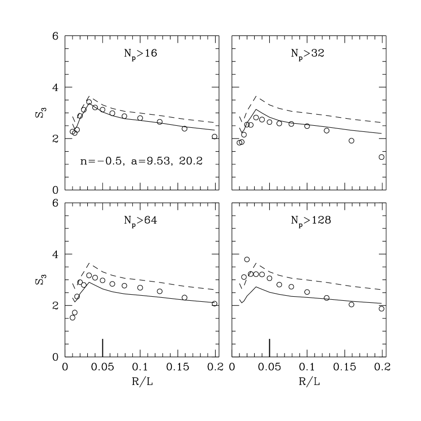
Figure 3c: The same as Fig. 3a for a model with $n=-0.5$.

Figure 3d: The same as Fig. 3a for halos selected at the same epoch as the one when skewness is calculated.

Figure 4a: The kurtosis of dark halos with different masses (indicated by $N_{p}$, the number of particles contained in the halos) predicted by our model (solid curves) compared with that derived from N-body simulations (circles). The dashed curves show the kurtosis of the mass density distribution in the simulation. Results are shown for scale-free model with $n=-1.5$. Halos are selected at an earlier epoch (when the expansion factor $a$ has the lower value indicated in the first panel) than when the kurtosis is calculated (at the epoch with the higher $a$). The thick ticks on the horizontal axis show the values of $R$ where ${\overline{\xi}}_{2}(R)=1$.

Figure 4b: The same as Fig. 4a for halos selected at another epoch.

Figure 4c: The same as Fig. 4a for a model with $n=-0.5$.

Figure 4d: The same as Fig. 4a for halos selected at the same epoch as the one when kurtosis is calculated.

Figure 5: Model predictions for the high order moments $S_{j,g}$ ($j=3$, 4 and 5) of halos (left panels) and peaks (right panels) at a radius $r=10\,h^{-1}{\rm{Mpc}}$ as a function of the linear bias parameter $b\equiv b_{1}$. Each curve shows result for a given $\delta_{1}$ (the linear overdensity of halos and peaks). Results are shown for $z_{1}\equiv(\delta_{1}/1.68-1)=0$, 0.5, 1, 2 and 4 (curves from bottom up). The horizontal lines show the values of $S_{j}$ for the mass density field calculated from quasilinear theory, whereas the data points (plotted arbitrarily at $b=2$) show the observational results for APM galaxies (Gaztanaga 1994).

References

- (1) Bahcall N. A., West M., 1992, ApJ, 392, 419
- (2) Bardeen J., Bond J.R., Kaiser N., Szalay A.S., 1986, ApJ, 304, 15 (BBKS)
- (3) Baugh C.M., Gaztanaga E., Efstathiou G., 1995, MNRAS, 274, 1049
- (4) Bernardeau F., 1992, ApJ, 392, 1
- (5) Bernardeau F., 1994, A&A, 291, 697
- (6) Bond J.R., Cole S., Efstathiou G., Kaiser N., 1991, ApJ, 379, 440
- (7) Bower R.J., 1991, MNRAS, 248, 332
- (8) Bouchet F.R., Strauss M., Davis M., Fisher K., Yahil A., Huchra J., 1993, ApJ, 417, 36
- (9) Cappi A., Maurogordato S., 1995, ApJ, 438, 507
- (10) Dalton G.B., Croft R.A.C., Efstathiou, G.,Sutherland W.J., Maddox S.J., Davis M., 1994, MNRAS, 271, L47
- (11) Davis M., Efstathiou G., Frenk C., White S.D.M., 1985, ApJ, 292, 371
- (12) Efstathiou G., Frenk C.S., White S.D.M., Davis M., 1988, MNRAS, 235, 715
- (13) Efstathiou G., Sutherland W.J., Maddox S.J., 1990, Nat, 348, 705
- (14) Frenk C.S., 1991, Physica Scripta, T36, 70
- (15) Frenk C.S., White S.D.M., Davis M., Efstathiou G., 1988, ApJ, 327, 507
- (16) Fry J.N., 1984, ApJ, 279, 499
- (17) Fry J.N., Gaztanaga E., 1993, ApJ, 413, 447
- (18) Gaztanaga E., 1994, MNRAS, 268, 913
- (19) Gaztanaga E., Croft R.A.C., Dalton G.B., 1995, MNRAS, 276, 336
- (20) Gaztanaga E., Frieman J.A., 1994, ApJ, 437, L13
- (21) Gelb J.M., Bertschinger E., 1994, ApJ, 436, 491
- (22) Lucchin F., Matarrese S., Melott A.L., Moscardini L., 1994, ApJ, 422, 430
- (23) Jain B., Mo H.J., White S.D.M., 1995, MNRAS, 276, L25
- (24) Jing Y.P., Mo H.J., Börner G., 1991, A&A, 252, 449
- (25) Jing Y.P., Mo H.J., Börner G., Fang L.Z., 1994, A&A, 284, 703
- (26) Jing Y.P., Zhang J.L., 1989, ApJ, 342, 639
- (27) Juszkiewicz R., Bouchet F., Colombi S., 1993, ApJ, 412, L9
- (28) Kaiser N., 1984, ApJ, 284, L9
- (29) Katz N., Quinn T., Gelb J.M., 1993, MNRAS, 265, 689
- (30) Kauffmann G., Nusser A., Steinmetz M., MNRAS, submitted
- (31) Kauffmann G., White S.D.M., 1993, MNRAS, 261, 921
- (32) Lacey C., Cole S., 1993, MNRAS, 262, 627
- (33) Lacey C., Cole S., 1994, MNRAS, 271, 676
- (34) Maddox S., et al., 1996, preprint
- (35) Meiksin A., Szapudi I., Szalay A.S., 1992, ApJ, 394, 87
- (36) Mo H.J., Jing Y.P., White S.D.M., 1996, MNRAS, submitted
- (37) Mo H.J., White S.D.M., 1996, MNRAS, in press
- (38) Nichol R.C., Collins C.A., Guzzo L., Lumsden S.L., 1992, MNRAS, 255, 21P
- (39) Peacock J.A., West M.J., 1992, MNRAS, 259, 494
- (40) Peebles P.J.E., 1980, The Large-Scale Structure of the Universe,Princeton University Press, Princeton
- (41) Plionis M., Valdarnini R., 1995, MNRAS, 272, 869
- (42) Press W.H., Schechter P., 1974, ApJ, 187, 425 (PS)
- (43) White S.D.M., Frenk C.S., 1991, ApJ, 379, 52
- (44) White S.D.M., Frenk C.S., Davis M., Efstathiou G., 1987, ApJ, 313, 505
- (45) White S.D.M., Rees M.J., 1978, MNRAS, 183, 341