Gravitational waves from pulsars: emission by the magnetic field induced distortion

Abstract

The gravitational wave emission by a distorted rotating fluid star is computed. The distortion is supposed to be symmetric around some axis inclined with respect to the rotation axis. In the general case, the gravitational radiation is emitted at two frequencies: $\Omega$ and $2\Omega$, where $\Omega$ is the rotation frequency. The obtained formulæ  are applied to the specific case of a neutron star distorted by its own magnetic field. Assuming that the period derivative $\dot{P}$ of pulsars is a measure of their magnetic dipole moment, the gravitational wave amplitude can be related to the observable parameters $P$ and $\dot{P}$ and to a factor $\beta$ which measures the efficiency of a given magnetic dipole moment in distorting the star. $\beta$ depends on the nuclear matter equation of state and on the magnetic field distribution. The amplitude at the frequency $2\Omega$, expressed in terms of $P$, $\dot{P}$ and $\beta$, is independent of the angle $\alpha$ between the magnetic axis and the rotation axis, whereas at the frequency $\Omega$, the amplitude increases as $\alpha$ decreases. The value of $\beta$ for specific models of magnetic field distributions has been computed by means of a numerical code giving self-consistent models of magnetized neutron stars within general relativity. It is found that the distortion at fixed magnetic dipole moment is very dependent of the magnetic field distribution; a stochastic magnetic field or a superconductor stellar interior greatly increases $\beta$ with respect to the uniformly magnetized perfect conductor case and might lead to gravitational waves detectable by the VIRGO or LIGO interferometers. The amplitude modulation of the signal induced by the daily rotation of the Earth has been computed and specified to the case of the Crab pulsar and VIRGO detector.

Key words: gravitation – magnetic fields – gravitational radiation – stars: neutron – pulsars: general – numerical methods: spectral

1 Introduction

Rapidly rotating neutron stars (pulsars) might be an important source of continuous gravitational waves in the frequency bandwidth of the forthcoming LIGO and VIRGO interferometric detectors (cf. Bonazzola & Marck 1994 for a recent review about the astrophysical sources these detectors may observe). It is well known that a stationary rotating body, perfectly symmetric with respect to its rotation axis does not emit any gravitational wave. Thus in order to radiate gravitationally a pulsar must deviate from axisymmetry. Various kinds of pulsar asymmetries have been suggested in the literature: first the crust of a neutron star is solid, so that its shape may not be necessarily axisymmetric under the effect of rotation, as it would be for a fluid: deviations from axisymmetry are supported by anisotropic stresses in the solid. The shape of the crust depends not only on the geological history of the neutron star, especially on the episode of crystallization of the crust, but also on star quakes. Due to its violent formation (supernova) or due to its environment (accretion disk), the rotation axis may not coincide with a principal axis of the neutron star moment of inertia and the star may precess (Pines & Shaham 1974). Even if it keeps a perfectly axisymmetric shape, a freely precessing body radiates gravitational waves (Zimmermann & Szedenits 1979). Neutron stars are known to have important magnetic fields; magnetic pressure (Lorentz forces exerted on the conducting matter) can distort the star if the magnetic axis is not aligned with the rotation axis, which is widely supposed to occur in order to explain the pulsar phenomenon. Another mechanism for producing asymmetries is the development of non-axisymmetric instabilities in rapidly rotating neutron stars driven by the gravitational radiation reaction (CFS instablity, cf. e.g. Schutz 1987) or by nuclear matter viscosity (cf. e.g. Bonazzola, Frieben & Gourgoulhon 1996 and references therein).

In the seventies it was widely thought that the solid part of neutron stars was large (see Sect.III of Goldreich 1970). A rotating rigid body whose rotation axis does not coincide with a principal axis of the moment of inertia must have a precessional motion. Therefore, there have been a number of studies about the precession of neutron stars and the resulting gravitational wave emission (Zimmermann 1978, Zimmermann & Szedenits 1979, Zimmermann 1980, Alpar & Pines 1985, Barone et al. 1988, de Araujo et al. 1994). However, modern dense matter calculations reveal that neutron star interiors are completely liquid (see e.g. Haensel 1995). Since the crust represents only 1 to 2% of the stellar mass (Lorenz et al. 1993), it appears that most of the neutron star is in a liquid phase. In this case, the star is not expected to precess, or at least its precession frequency must be reduced by a factor $10^{5}$ as compared with the solid case (Pines & Shaham 1974).

The gravitational radiation from a rotating fluid star has not been studied as much as that from a solid star. The only reference we are aware of is the work by Gal’tsov, Tsvetkov & Tsirulev (1984) and by Gal’tsov & Tsvetkov (1984) about the gravitational emission of a rotating Newtonian homegeneous fluid drop with an oblique magnetic field. These authors have shown that the gravitational waves are emitted at two frequencies: the rotation frequency and twice the rotation frequency. They did not give explicit formulæ for the two gravitational wave amplitude $h_{+}$ and $h_{\times}$ but have instead computed the response of a heterodyne detector (consisting in a rotating dumbbell orientated at right angles to the direction of propagation of the wave) directly from the Riemann tensor.

In the present article, we compute the gravitational radiation from a rotating fluid star, distorted along a certain direction by some process (for example an internal magnetic field), the angle between this direction and the rotation axis being arbitrary (Sect.2). We do not assume that the star is a Newtonian object: it can have a large gravitational field described by the theory of general relativity — which is relevant for neutron stars. As an illustration we give the specific example of a Newtonian incompressible fluid with a uniform internal magnetic field (Sect.3). We consider also the (more general) case where the deformation is due to an internal magnetic field which is also responsible for the $\dot{P}$ of the pulsar (electromagnetic braking) (Sect.4). Using the numerical code presented in (Bocquet, Bonazzola, Gourgoulhon & Novak 1995) for magnetized rotating neutron stars in general relativity, we compute the gravitational emission for a specific $1.4\,M_{\odot}$ neutron star model and for various configurations of the internal magnetic field. Finally, we derive the response of an interferometric detector to the gravitational signal, taking into account the daily change induced by the Earth rotation in the relative orientation of the detector arms and the source (Sect.5).

2 Generation of gravitational waves by a rotating fluid star

2.1 Thorne’s quadrupole moment

Neutron stars are fully relativistic objects, so that the standard quadrupole formula for gravitational wave generation — which is derived for non relativistic sources (cf. Sect.36.10 of Misner, Thorne & Wheeler 1973, hereafter MTW) — does not a priori apply. However Ipser (1971) has shown that the gravitational radiation from a slowly rotating and fully relativistic star is given by a formula structurally identical to the weak field standard formula, provided that the involved multipole moments are defined in an appropriate way.

The leading term in the gravitational radiation field is then given by the formula:

$$h_{ij}^{\rm TT}={2G\over c^{4}}\,{1\over r}\,\left[P_{i}^{\ \,k}P_{j}^{\ \,l}-{1\over 2}P_{ij}P^{kl}\right]{\ddot{\cal I}}_{kl}\left(t-{r\over c}\right)\ ,$$ (1)

where $r$ is the distance to the source and $P_{ij}:=\delta_{ij}-r_{i}r_{j}/r^{2}$ is the tensor of projection transverse to the line of sight. Eq.(1) holds for highly relativistic sources provided that ${\cal I}_{ij}$ is the mass quadrupole moment defined as the quadrupolar part of the $1/r^{3}$ term of the $1/r$ expansion of the metric coefficient $g_{00}$ in an asymptotically Cartesian and mass centered (ACMC) coordinate system (Thorne 1980). This latter is a very broad coordinate class, which includes the harmonic coordinates. The precise definition of ${\cal I}_{ij}$ is the following one. The space around a neutron star of mass $M$, “typical” radius $R$ and angular velocity $\Omega$ can be divided in three regions:

• the strong-field region: $r\mathrel{\hbox to0.0pt{\lower 3.0pt\hbox{$\mathchar 536\relax$}\hss}\raise 2.0pt\hbox{$\mathchar 316\relax$}}\mbox{a few}\ {GM/c^{2}}$;

• the weak-field near zone: $\max(R,\ \mbox{a few}\ {GM/c^{2}})\mathrel{\hbox to0.0pt{\lower 3.0pt\hbox{$\mathchar 536\relax$}\hss}\raise 2.0pt\hbox{$\mathchar 316\relax$}}r\mathrel{\hbox to0.0pt{\lower 3.0pt\hbox{$\mathchar 536\relax$}\hss}\raise 2.0pt\hbox{$\mathchar 316\relax$}}c/\Omega$

• the wave zone : $r\mathrel{\hbox to0.0pt{\lower 3.0pt\hbox{$\mathchar 536\relax$}\hss}\raise 2.0pt\hbox{$\mathchar 318\relax$}}c/\Omega$

In the wave zone, retardation effects are important whereas in the weak-field near zone, the gravitational field can be considered as quasi-stationary. Note that for the fastest millisecond pulsar to date, PSR 1937+21, $c/\Omega\sim 80\ {\rm km}$, whereas $R\sim 10{\ \rm km}$ and if its mass is $M=1.4M_{\odot}$, $GM/c^{2}\sim 2\ {\rm km}$. Hence, even in this extreme case, the weak-field near zone is well defined. A coordinate system $(t,x^{1},x^{2},x^{3})$ is said to be asymptotically Cartesian and mass centered (ACMC) to order 1 if the metric admits the following $1/r$ expansion ($r:=x_{i}x^{i}$) in the weak-field near zone (Sect.XI of Thorne 1980):

$$g_{00} = -1+{2M\over r}+{\alpha_{1}\over r^{2}}$$ (2)

$$+{1\over r^{3}}\left[3\,{\cal I}_{ij}{x^{i}x^{j}\over r^{2}}+\beta_{1i}{x^{i}\over r}+\alpha_{2}\right]+O\left({1\over r^{4}}\right)$$

$$g_{0i} = -4\epsilon_{ikl}J^{k}{x^{l}\over r^{3}}+O\left({1\over r^{3}}\right)$$ (3)

$$g_{ij} = \delta_{ij}+{\alpha_{3ij}\over r}+{1\over r^{2}}\left[\beta_{2ijk}{x^{k}\over r}+\alpha_{4ij}\right]+O\left({1\over r^{3}}\right)\ ,$$ (4)

where $\alpha_{1}$, $\alpha_{2}$, $\alpha_{3ij}$, $\alpha_{4ij}$, $\beta_{1i}$ and $\beta_{2ijk}$ are some constants. The coefficients $M$ and $J^{k}$ in the above expansion are the star’s total mass and angular momentum. They are independent of the $(x^{i})$ coordinate choice, provided that they reduce to usual Cartesian coordinates at the asymptotically flat infinity. On the contrary, the coefficient ${\cal I}_{ij}$ is not invariant under change of asymptotically Cartesian coordinates: it is invariant only with respect to the sub-class of ACMC coordinates. This quantity is called the mass quadrupole moment of the star. As discussed in Sect.XI of Thorne (1980) (cf. also Thorne & Gürsel 1983), ${\cal I}_{ij}$ is a flat-space-type tensor which “resides” in the weak-field near zone, which means that it can be manipulated as a tensor in flat space. This tensor is symmetric and trace-free. If the star has a gravitational field weak enough to be correctly described by the Newtonian theory of gravitation, ${\cal I}_{ij}$ is expressible as minus the trace-free part of the moment of inertia tensor $I_{ij}$:

$${\cal I}_{ij}=-I_{ij}+{1\over 3}I_{k}^{\ k}\,\delta_{ij}\ ,$$ (5)

$I_{ij}$ being given by

$$I_{ij}:=\int\rho\left(x_{k}x^{k}\,\delta_{ij}-x_{i}x_{j}\right)d^{3}x\ .$$ (6)

In particular, ${\cal I}_{ij}$ coincides at the Newtonian limit with the quantity $-\!\!\!\!I_{ij}$ introduced in MTW. For highly relativistic configurations, ${\cal I}_{ij}$ can no longer be expressed as some integral over the star, as in Eqs.(5)-(6); it must be read from the $1/r$ expansion of the metric coefficient $g_{00}$ in an ACMC coordinate system. In Appendix A, we give the transformation from a quasi-isotropic coordinate system, usually used in relativistic studies of rotating neutron stars (cf the discussion in Sect2 of Bonazzola, Gourgoulhon, Salgado & Marck 1993), to an ACMC coordinate system.

2.2 Slightly deformed rotating star

Very tight limits have been set on the deformation of neutron stars by pulsar timings: the relative deviation from axisymmetry is at most $10^{-3}$ (cf. Table1 of New et al. 1995). This number is certainly overestimated by several orders of magnitude for it is obtained by assuming that all the observed period derivative $\dot{P}$ is due to the gravitational emission, whereas it is much more likely to be due to the electromagnetic emission. Indeed, the present measurements of the braking index $n$ of pulsars are $n=2.509\pm 0.001$ for the Crab, $n=2.01\pm 0.02$ for PSR 0540-69 and $n=2.837\pm 0.001$ for PSR 1509-58 (cf. Muslimov & Page 1996 for references). Thus they are closer to $n=3$ (magnetic dipole radiation) than to $n=5$ (gravitational radiation, cf. Table9.1 of Manchester & Taylor 1977).

For such small deformations, we make the assumption that the quadrupole moment ${\cal I}_{ij}$ can be linearly decomposed into the sum of two pieces:

$${\cal I}_{ij}={\cal I}_{ij}^{\rm rot}+{\cal I}_{ij}^{\rm dist}\ ;$$ (7)

${\cal I}_{ij}^{\rm rot}$ is the quadrupole moment due to rotation: ${\cal I}_{ij}^{\rm rot}=0$ if the configuration is static. ${\cal I}_{ij}^{\rm dist}$ is the quadrupole moment due to some process that distorts the star, for example an internal magnetic field or anisotropic stresses for the nuclear interactions.

The fact that the star does not precess implies that there exists some ACMC coordinate system $x^{\alpha}=(t,x,y,z)$ such that the components ${\cal I}_{ij}^{\rm rot}$ in this coordinate system do not depend upon $x^{0}=t$ and take the diagonal form

$${\cal I}_{ij}^{\rm rot}=\left(\begin{array}[]{ccc}-{\cal I}_{zz}^{\rm rot}/2&0&0\\ 0&-{\cal I}_{zz}^{\rm rot}/2&0\\ 0&0&{\cal I}_{zz}^{\rm rot}\end{array}\right)\ .$$ (8)

The line $x=y=0$ is the rotation axis. For a small angular velocity $\Omega$, ${\cal I}_{zz}^{\rm rot}$ is a quadratic function of $\Omega$.

Let us make the following assumptions about the distortion process:

1. there exists some privileged direction, i.e. two of the three eigenvalues of ${\cal I}_{ij}^{\rm dist}$ are equal, i.e. there exists in the weak-field near zone a coordinate system (not necessarily ACMC) $x^{\hat{\alpha}}=(\hat{t},\hat{x},\hat{y},\hat{z})$ such that the components ${\cal I}_{\hat{i}\hat{j}}^{\rm dist}$ are

   $${\cal I}_{\hat{i}\hat{j}}^{\rm dist}=\left(\begin{array}[]{ccc}-{\cal I}_{\hat{z}\hat{z}}^{\rm dist}/2&0&0\\ 0&-{\cal I}_{\hat{z}\hat{z}}^{\rm dist}/2&0\\ 0&0&{\cal I}_{\hat{z}\hat{z}}^{\rm dist}\end{array}\right)\ .$$ (9)

2. the deformation is rotating with the star, i.e. the weak-field near zone vector ${\bf e}_{\hat{z}}$ associated with the coordinate $\hat{z}$ is rotating at the angular velocity $\Omega$ at a fixed angle $\alpha$ from the weak-field near zone vector ${\bf e}_{z}$ associated with the coordinate $z$ (${\bf e}_{z}$ is along the rotation axis) (cf. Fig.1):

   $${\bf e}_{\hat{z}}=\cos\alpha\,{\bf e}_{z}+\sin\alpha\left[\cos\varphi(t)\,{\bf e}_{x}+\sin\varphi(t)\,{\bf e}_{y}\right]\ ,$$ (10)

   with

   $$\varphi(t)=\Omega(t-t_{0})\ .$$ (11)

In particular, the above assumptions are satisfied by a magnetic field symmetric with respect to some axis: ${\bf e}_{\hat{z}}$ is then parallel to the magnetic dipole moment vector $\cal M$.

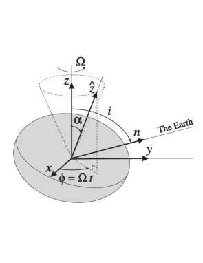
Fig. 1.: Geometry of the distorted neutron star.

2.3 Application of the quadrupole formula

Inserting Eq.(7) into the quadrupole formula (1) and using the time constancy of ${\cal I}_{ij}^{\rm rot}$, we get

$$h_{ij}^{\rm TT}={2G\over c^{4}}\,{1\over r}\,\left[P_{i}^{\ \,k}P_{j}^{\ \,l}-{1\over 2}P_{ij}P^{kl}\right]{\ddot{\cal I}}_{kl}^{\rm dist}\left(t-{r\over c}\right)\ .$$ (12)

In order to apply this formula, one must first express ${\cal I}_{ij}^{\rm dist}$ in the ACMC coordinates $(t,x,y,z)$, from its components (9) in the coordinates $(\hat{t},\hat{x},\hat{y},\hat{z})$. The transformation $(\hat{t},\hat{x},\hat{y},\hat{z})\rightarrow(t,x,y,z)$ is simply the composition of two rotations (cf. Fig.1): one of angle $\alpha$ around an axis ${\bf e}_{x^{\prime}}$ in the $({\bf e}_{x},{\bf e}_{y})$ plane and rotating with the star, and one of angle $\varphi(t)=\Omega(t-t_{0})$ around ${\bf e}_{z}$. The transformation matrix is then:

$$P=\left(\begin{array}[]{ccc}\cos\varphi(t)&-\sin\varphi(t)&0\\ \sin\varphi(t)&\cos\varphi(t)&0\\ 0&0&1\end{array}\right)\times\left(\begin{array}[]{ccc}1&0&0\\ 0&\cos\alpha&\sin\alpha\\ 0&-\sin\alpha&\cos\alpha\end{array}\right).$$ (13)

The tensor transformation law writes ${\cal I}^{\rm dist}=P\times\hat{\cal I}^{\rm dist}\times{}^{t}P$, where ${\cal I}^{\rm dist}$ is the matrix formed by the components ${\cal I}_{ij}^{\rm dist}$ and $\hat{\cal I}^{\rm dist}$ is the matrix formed by the components ${\cal I}_{\hat{i}\hat{j}}^{\rm dist}$ [Eq.(9)]. Performing this matrix product leads to

$${\cal I}_{ij}^{\rm dist}\!\!\! ={1\over 2}{\cal I}_{\hat{z}\hat{z}}^{\rm dist}\left(\begin{array}[]{c}3\sin^{2}\alpha\sin^{2}\varphi(t)-1\\ -3/2\,\sin^{2}\alpha\sin 2\varphi(t)\\ -3\sin\alpha\cos\alpha\sin\varphi(t)\end{array}\right.$$ (21)

$$\left.\begin{array}[]{cc}-3/2\,\sin^{2}\alpha\sin 2\varphi(t)&-3\sin\alpha\cos\alpha\sin\varphi(t)\\ 3\sin^{2}\alpha\cos^{2}\varphi(t)-1&3\sin\alpha\cos\alpha\cos\varphi(t)\\ 3\sin\alpha\cos\alpha\cos\varphi(t)&3\cos^{2}\alpha-1\end{array}\right).$$

In order to apply the quadrupole formula, the second derivative with respect to $t$ of this expression must be taken. One obtains, using Eq.(11),

$${\ddot{\cal I}}_{ij}^{\rm dist}\!\!\! ={3\over 2}{\cal I}_{\hat{z}\hat{z}}^{\rm dist}\,\Omega^{2}\sin\alpha\left(\begin{array}[]{c}2\sin\alpha\cos 2\varphi(t)\\ 2\sin\alpha\sin 2\varphi(t)\\ \cos\alpha\sin\varphi(t)\end{array}\right.$$ (29)

$$\qquad\qquad\left.\begin{array}[]{cc}2\sin\alpha\sin 2\varphi(t)&\cos\alpha\sin\varphi(t)\\ -2\sin\alpha\cos 2\varphi(t)&-\cos\alpha\cos\varphi(t)\\ -\cos\alpha\cos\varphi(t)&0\end{array}\right).$$

The next step consists in taking the transverse traceless projection of ${\ddot{\cal I}}_{ij}^{\rm dist}$. Let us denote by $i$ the angle between the neutron star’s rotation axis ${\bf e}_{z}$ and the direction ${\bf n}$ from the star’s centre to the Earth ($i$ is called the line of sight inclination) (cf. Fig.1). Without any loss of generality, we can choose the ACMC coordinates $(t,x,y,z)$ such that ${\bf n}$ lies in the $({\bf e}_{y},{\bf e}_{z})$ plane. The components with respect to $(t,x,y,z)$ of the transverse projection operator $P_{ij}=\delta_{ij}-n_{i}n_{j}$ are then

$$P_{ij}=\left(\begin{array}[]{ccc}1&0&0\\ 0&\cos^{2}i&-\sin i\cos i\\ 0&-\sin i\cos i&\sin^{2}i\end{array}\right)\ .$$ (30)

From Eqs.(30) and (29), the computation of the right-hand side of the quadrupole formula (12) is straightforward, though somewhat tedious. The result is

$$h_{ij}^{\rm TT}=h_{+}\,e_{ij}^{+}\ +\ h_{\times}\,e_{ij}^{\times}\ ,$$ (31)

with

$$e_{ij}^{+} = \left(\begin{array}[]{ccc}1&0&0\\ 0&-\cos^{2}i&\sin i\cos i\\ 0&\sin i\cos i&-\sin^{2}i\end{array}\right)\ ,$$ (35)

$$e_{ij}^{\times} = \left(\begin{array}[]{ccc}0&\cos i&-\sin i\\ \cos i&0&0\\ -\sin i&0&0\end{array}\right)$$ (39)

and

$$h_{+} = h_{0}\sin\alpha\Big{[}{1\over 2}\cos\alpha\sin i\cos i\cos\Omega(t-t_{0})$$ (40)

$$\qquad\qquad-\sin\alpha{1+\cos^{2}i\over 2}\cos 2\Omega(t-t_{0})\Big{]}$$

$$h_{\times} = h_{0}\sin\alpha\Big{[}{1\over 2}\cos\alpha\sin i\sin\Omega(t-t_{0})$$ (41)

$$\qquad\qquad-\sin\alpha\cos i\sin 2\Omega(t-t_{0})\Big{]}\ ,$$

where

$$h_{0}:=-{6G\over c^{4}}{\cal I}_{\hat{z}\hat{z}}^{\rm dist}{\Omega^{2}\over r}\ .$$ (42)

Note that in the above expressions, Eq.(11) has been substituted for $\varphi(t)$ and that the retardation term $-r/c$ has been incorporated into the constant $t_{0}$.

2.4 Discussion

From the formulæ (40)-(41), it is clear that there is no gravitational emission if the distortion axis is aligned with the rotation axis ($\alpha=0\ \mbox{or}\ \pi$). If both axes are perpendicular ($\alpha=\pi/2$), the gravitational emission is monochromatic at twice the rotation frequency. In the general case ($0<|\alpha|<\pi/2$), it contains two frequencies: $\Omega$ and $2\Omega$. For small values of $\alpha$ the emission at $\Omega$ is dominant.

It may be noticed that Eqs.(40)-(42) are structurally equivalent to Eq.(1) of Zimmermann & Szedenits (1979) (hereafter ZS), although this latter work is based on a different physical hypothesis (Newtonian precessing rigid star). In order to compare precisely Eqs.(40)-(42) and Eq.(1) of ZS, some slight re-arrangements must be performed. First, the ellipticity $\epsilon$ defined by ZS is linked to our ${\cal I}_{\hat{z}\hat{z}}$ by $I_{1}\epsilon=-3/2\,{\cal I}_{\hat{z}\hat{z}}$ [cf. Eq.(5)], this explains the factor 2 in front of the right-hand side of Eq.(1) of ZS instead of the factor $-6$ in Eq.(42). Other apparent differences are actually due to different conventions: the origin of time in ZS is the instant when the equivalent of the deformation axis is at its farthest position from the observer, whereas in our case it corresponds to its nearest position. One must then make $t\rightarrow t+\pi$ in order to compare the two formulæ. Moreover the choice for the matrices $e_{ij}^{+}$ and $e_{ij}^{\times}$ are exactly opposite in both approaches [cf. Sect.III.B of Zimmermann (1980)], so that the transforms $h_{+}\rightarrow-h_{+}$ and $h_{\times}\rightarrow-h_{\times}$ must also be performed. When all this is done, Eqs.(40)-(42) and Eq.(1) of ZS appear to have exactly the same structure. However, the physical significance is different: the frequency $\omega$ which appears in Eq.(1) of ZS differs from the pulsar frequency by the body-frame precessional frequency whereas in Eqs.(40)-(42), $\Omega$ is exactly the pulsar frequency. The angle $\theta$ of ZS, which in their Eq.(1) takes the place of our angle $\alpha$ in Eqs.(40)-(42), is the angle between the total angular momentum ${\bf J}$ and the star’s third principal axis, whereas our $\alpha$ is the angle between the rotation axis and the direction of the distortion, which even in the Newtonian case, does not coincide with any of the principal axis of the body (except in the non-rotating case).

As special cases of Eqs.(40)-(42), one may recover results previously published in the literature. For instance, the case of a triaxial star rotating about a principal axis of its moment of inertia tensor can be obtained by setting $\alpha=\pi/2$ in Eqs.(40)-(42). The result can be compared with Eqs.(48) and (54) of Thorne (1987), noticing that $f$ in these equations is $\Omega/\pi$ and that ${\cal I}_{\bar{x}\bar{x}}$ and ${\cal I}_{\bar{y}\bar{y}}$ of Thorne (1987) are related to our ${\cal I}_{\hat{z}\hat{z}}$ by ${\cal I}_{\bar{x}\bar{x}}=-{\cal I}_{\hat{z}\hat{z}}/2$ and ${\cal I}_{\bar{y}\bar{y}}={\cal I}_{\hat{z}\hat{z}}$. The two formulæ appear then to be identical, as expected. If in addition to $\alpha=\pi/2$, the inclination angle $i$ is set to zero, Eqs.(40)-(42) reduce to the formula used in the recent work by New et al. (1995) [their Eq.(5)]. Note that in the two studies mentionned above, the gravitational waves are emitted at the frequency $2\Omega$ only, due to $\alpha=\pi/2$ or equivalently due to the fact that the rotation axis coincides with a principal axis of the moment of inertia tensor. Let us stress again that in our (more general) case, the gravitational radiation contains two frequencies: $\Omega$ and $2\Omega$.

2.5 Numerical estimates

In order to describe the star deformation by a dimensionless quantity, let us introduce instead of ${\cal I}_{\hat{z}\hat{z}}^{\rm dist}$ the ellipticity

$$\epsilon:=-{3\over 2}\,{{\cal I}_{\hat{z}\hat{z}}^{\rm dist}\over I}\ ,$$ (43)

where $I$ is the moment of inertia with respect to the rotation axis, defined as

$$I:=J/\Omega\ ,$$ (44)

$J$ being the star angular momentum. The definition (44) is valid even in highly relativistic cases, provided that the star distortion is small — as we suppose throughout this work. Indeed, in this case the configuration is essentially axisymmetric and the angular momentum $J$ is well defined (cf. e.g. the discussion in Wald (1984), p. 297). The factor $-3/2$ in Eq.(43) is introduced in order to recover the classical definition of the ellipticity at the Newtonian limit (see e.g. Shapiro & Teukolsky 1983).

Let us introduce also the rotation period $P={2\pi/\Omega}$, since observational data about pulsars are usually presented with $P$ instead of $\Omega$.

Inserting Eq.(43) in expression (42) for the characteristic gravitational wave amplitude leads to

$$h_{0}={16\pi^{2}G\over c^{4}}{I\,\epsilon\over P^{2}\,r}\ .$$ (45)

Replacing the physical constants by their numerical values results in

$$h_{0}=4.21\times 10^{-24}\ \Big{[}{{\rm ms}\over P}\Big{]}^{2}\Big{[}{{\rm kpc}\over r}\Big{]}\Big{[}{I\over 10^{38}{\ \rm kg\,m}^{2}}\Big{]}\Big{[}{\epsilon\over 10^{-6}}\Big{]}.$$ (46)

Note that $I=10^{38}{\ \rm kg\,m}^{2}$ is a representative value for the moment of inertia of a $1.4\,M_{\odot}$ neutron star [see Fig.12 of Arnett & Bowers (1977)].

For the Crab pulsar, $P=33{\ \rm ms}$ and $r=2{\ \rm kpc}$, so that Eq.(46) becomes

$$h_{0}^{\rm Crab}=1.89\times 10^{-27}\Big{[}{I\over 10^{38}{\ \rm kg\,m}^{2}}\Big{]}\Big{[}{\epsilon\over 10^{-6}}\Big{]}.$$ (47)

For the Vela pulsar, $P=89{\ \rm ms}$ and $r=0.5{\ \rm kpc}$, hence

$$h_{0}^{\rm Vela}=1.06\times 10^{-27}\Big{[}{I\over 10^{38}{\ \rm kg\,m}^{2}}\Big{]}\Big{[}{\epsilon\over 10^{-6}}\Big{]}.$$ (48)

For the millisecond pulsar PSR 1957+20, $P=1.61{\ \rm ms}$ and $r=1.5{\ \rm kpc}$, hence

$$h_{0}^{\mbox{1957+20}}=1.08\times 10^{-24}\Big{[}{I\over 10^{38}{\ \rm kg\,m}^{2}}\Big{]}\Big{[}{\epsilon\over 10^{-6}}\Big{]}.$$ (49)

At first glance, PSR 1957+20 seems to be a much more favorable candidate than the Crab or Vela. However, in the above formula, $\epsilon$ is in units of $10^{-6}$ and the very low value of the period derivative $\dot{P}$ of PSR 1957+20 implies that its $\epsilon$ is at most $1.6\times 10^{-9}$ (New et al. 1995). Hence the maximum amplitude one can expect for this pulsar is $h_{0}^{\mbox{1957+20}}\sim 1.7\times 10^{-27}$ and not $1.08\times 10^{-24}$ as Eq.(49) might suggest.

3 The incompressible magnetized fluid example

As an illustration, let us consider the specific example taken by Gal’tsov, Tsvetkov & Tsirulev (1984) (hereafter GTT) and Gal’tsov & Tsevtkov (1984). In their work, a pulsar is idealized as a rigidly rotating Newtonian body made of an incompressible fluid and endoved with a magnetic field which is uniform inside the star and dipolar oustide it, the magnetic dipole moment being inclined by an angle $\alpha$ with respect to the rotation axis.

The rotation rate is supposed to be far from the mass-shedding limit so that the departure from spherical symmetry is small. Moreover, the magnetic energy is assumed to be much lower than the rotational kinetic energy, which is satisfied by realistic configurations. Under these hypotheses, the star takes the shape of a (quasi-spherical) triaxial ellipsoid. The gravitational potential can be then calculated from the analytical formulæ of Chandrasekhar (1969). The shape of the ellipsoid is deduced from the first integral of the equation of motion (including the magnetic pressure) and the magnetic field matching conditions at the stellar surface. It is found that the ellipsoid is determined by the equation $(\delta_{ij}+a_{ij})X^{i}X^{j}=R^{2}$, where (i) $R$ is the mean radius of the (quasi-spherical) ellipsoid, (ii) $X^{i}$ are Cartesian coordinates in a co-moving frame, i.e. rotating at the angular velocity $\Omega$ with respect to an inertial frame and (iii) the $a_{ij}$ are given by

$$a_{ij}={15\over 2}\,{\Omega_{i}\Omega_{j}\over\omega_{\rm J}^{2}}+{45\mu_{0}\over 32\pi^{2}}\,{{\cal M}_{i}{\cal M}_{j}\over R^{8}\rho\omega_{\rm J}^{2}}\ .$$ (50)

In this expression, $\rho$ is the constant mass density of the star, $\omega_{\rm J}=\sqrt{4\pi G\rho}$ is the Jeans frequency, $\Omega_{i}$ and ${\cal M}_{i}$ are respectively the components of the angular velocity vector and the components of the magnetic dipole moment with respect to the $X^{i}$ coordinates: $\Omega_{i}=(0,0,\Omega)$ and ${\cal M}_{i}=(0,{\cal M}\sin\alpha,{\cal M}\cos\alpha)$. By diagonalizing the matrix $a_{ij}$ given by Eq.(50), one obtains the principal axes of the ellipsoid and the values of the three semi-axes, $a_{1}$, $a_{2}$ and $a_{3}$. From these quantities the moment of inertia tensor $I_{ij}$ can be computed by evaluating the integral (6) in the frame of the principal axes. The quadrupole moment ${\cal I}_{ij}$ is then immediately deduced via Eq.(5). Transforming the result in the inertial frame leads to the form (7) of ${\cal I}_{ij}$, incidently demonstrating this formula in the particular case under consideration, with the form (8) for ${\cal I}_{ij}^{\rm rot}$ with

$${\cal I}_{zz}^{\rm rot}=-{R^{5}\Omega^{2}\over 3G}$$ (51)

and with the form (21) for ${\cal I}_{ij}^{\rm dist}$ with

$${\cal I}_{\hat{z}\hat{z}}^{\rm dist}=-{\mu_{0}{\cal M}^{2}\over 16\pi^{2}G\rho R^{3}}\ .$$ (52)

The moment of inertia with respect to the rotation axis of the homogeneous star is $I=8\pi\rho R^{5}/15$, so that Eq.(43) gives the ellipticity:

$$\epsilon={45\over 64\pi}{B_{\rm pole}^{2}\over\mu_{0}G\rho^{2}R^{2}}\ .$$ (53)

Note that in this formula, the magnetic dipole moment $\cal M$ has been expressed in terms of the North pole magnetic field $B_{\rm pole}=\mu_{0}/(4\pi)\,2{\cal M}/R^{3}$.

For numerical estimates, let us take typical values for neutron stars: $B_{\rm pole}=10^{9}$ T, $M=1.4\,M_{\odot}$ and $R=10$ km. Then $\epsilon\simeq 6.0\times 10^{-11}$. This is a very tiny value, which leads to a gravitational wave amplitude of only $h_{0}\sim 3\times 10^{-30}$ for $P=10$ ms and $r=1$ kpc [cf. Eq.(46)]. However the above model is a very simplified one. It can be expected that relaxing the assumptions of (i) incompressible fluid, (ii) Newtonian gravity and (iii) uniform internal magnetic field, may lead to a greater value of $\epsilon$.

4 Magnetic field induced deformation

4.1 Emission formula

The situation considered in the preceding section is a very simplified one. However, one may consider that the obtained form of the deformation, Eq.(52), is qualitatively the same for realistic magnetized neutron star models, i.e. a compressible perfect fluid obeying a “sophisticated” equation of state resulting from nuclear physics calculations, and involving general relativity. More precisely, we consider that the magnetic field induced deformation is a quadratic function of the amplitude of the magnetic dipole moment, $\cal M$, as in Eq.(52):

$$\epsilon=\beta\,{{\cal M}^{2}\over{\cal M}_{0}^{2}}\ ,$$ (54)

where ${\cal M}_{0}$ has the dimension of a magnetic dipole moment in order to make the coefficient $\beta$ dimensionless. Let us choose ${\cal M}_{0}^{2}=(4\pi/\mu_{0})\,GI^{2}/R^{2}$ where $R$ is the circumferential equatorial radius of the star. Hence

$$\epsilon=\beta\,{\mu_{0}\over 4\pi}{{\cal M}^{2}R^{2}\over G\,I^{2}}\ .$$ (55)

Provided the magnetic field amplitude does not take (unrealistic) huge values ($>10^{14}$ T), this formula is certainly true, even if the magnetic field structure is quite complicated, depending upon the assumed electromagnetic properties of the fluid: normal conductor, superconductor, ferromagnetic… The coefficient $\beta$ measures the efficiency of this magnetic structure in distorting the star. In the following, we shall call $\beta$ the magnetic distortion factor. For the simplified model considered in Sect.3 (incompressible fluid, uniform internal magnetic field), $\beta=1/5$.

As argued in Sect.2.2, the observed spin down of radio pulsars is very certainly due to the low frequency magnetic dipole radiation. $\cal M$ is then linked to the observed pulsar period $P$ and period derivative $\dot{P}$ by [cf e.g. Eq.(6.10.26) of Straumann (1984)]

$${\cal M}^{2}={4\pi\over\mu_{0}}{3c^{3}\over 8\pi^{2}}{IP\dot{P}\over\sin^{2}\alpha}\ ,$$ (56)

where $\alpha$ is the angle between the magnetic dipole moment $\cal M$ and the rotation axis. For highly relativistic configurations, the vector $\cal M$ is defined in the weak-field near zone (cf. Sect.2.5 of Bocquet et al. 1995), so is $\alpha$. Inserting Eqs.(55) and (56) into Eq.(45) leads to the gravitational wave amplitude

$$h_{0}=6\beta\,{R^{2}\dot{P}\over crP\sin^{2}\alpha}\ ,$$ (57)

so that formulæ (40) and (41) become

$$h_{+} = 6\beta\,{R^{2}\dot{P}\over crP}\Big{[}{\sin i\cos i\over 2\tan\alpha}\cos\Omega(t-t_{0})$$ (58)

$$\qquad\qquad\quad-{1+\cos^{2}i\over 2}\cos 2\Omega(t-t_{0})\Big{]}$$

$$h_{\times} = 6\beta\,{R^{2}\dot{P}\over crP}\Big{[}{\sin i\over 2\tan\alpha}\sin\Omega(t-t_{0})$$ (59)

$$\qquad\qquad\quad-\cos i\sin 2\Omega(t-t_{0})\Big{]}\ .$$

Equation (57) can be cast in a numerically convenient form:

$$h_{0}=6.48\times 10^{-30}\,{\beta\over\sin^{2}\alpha}\,\Big{[}{R\over 10{\,\rm km}}\Big{]}^{2}\Big{[}{{\rm kpc}\over r}\Big{]}\Big{[}{{\rm ms}\over P}\Big{]}\Big{[}{\dot{P}\over 10^{-13}}\Big{]}\ .$$ (60)

As a check of this equation, let us consider again the simplified case of Sect.3. The uniformly magnetized homogeneous Newtonian star with $M=1.4\,M_{\odot}$, $R=10\ {\rm km}$, $B_{\rm pole}=10^{9}\ {\rm T}$ and $P=10\ {\rm ms}$ has a moment of inertia $I=1.1\times 10^{38}\ {\rm kg\,m}^{2}$, a factor $\beta=1/5$, and magnetic dipole moment ${\cal M}=5.0\times 10^{27}\ {\rm A\,m}^{2}$. From Eq.(56), the corresponding period derivative is $\dot{P}=2.2\times 10^{-12}\,\sin^{2}\alpha$. Equation(60) gives then $h_{0}=3\times 10^{-30}$ for $r=1\ {\rm kpc}$, in agreement with the result obtained in Sect.3.

The main feature of the emission formulæ (58)-(59) is that the amplitude of the gravitational radiation at the frequency $2\Omega$ does not depend upon the (unknown) angle $\alpha$.

4.2 Discussion

Among the 706 pulsars of the catalog by Taylor et al. (1995, 1993), the highest value of $h_{0}$ at fixed $\alpha$, $\beta$ and $R$, as given by Eq.(60), is achieved by the Crab pulsar ($P=33{\ \rm ms}$, $\dot{P}=4.21\times 10^{-13}$, $r=2{\ \rm kpc}$), followed by Vela ($P=89{\ \rm ms}$, $\dot{P}=1.25\times 10^{-13}$, $r=0.5{\ \rm kpc}$) and PSR1509-58 ($P=151{\ \rm ms}$, $\dot{P}=1.54\times 10^{-12}$, $r=4.4{\ \rm kpc}$):

$$h_{0}^{\rm Crab} = 4.08\times 10^{-31}\Big{[}{R\over 10{\,\rm km}}\Big{]}^{2}\,{\beta\over\sin^{2}\alpha}$$ (61)

$$h_{0}^{\rm Vela} = 1.81\times 10^{-31}\Big{[}{R\over 10{\,\rm km}}\Big{]}^{2}\,{\beta\over\sin^{2}\alpha}$$ (62)

$$h_{0}^{\mbox{1509-58}} = 1.50\times 10^{-31}\Big{[}{R\over 10{\,\rm km}}\Big{]}^{2}\,{\beta\over\sin^{2}\alpha}$$ (63)

$$h_{0}^{\mbox{1957+20}} = 4.51\times 10^{-37}\Big{[}{R\over 10{\,\rm km}}\Big{]}^{2}\,{\beta\over\sin^{2}\alpha}\ .$$ (64)

We have added to the list the millisecond pulsar PSR 1957+20 ($P=1.61{\ \rm ms}$, $\dot{P}=1.68\times 10^{-20}$, $r=1.5{\ \rm kpc}$) considered in Sect.2.5. From the above values, it appears that PSR 1957+20 is not a good candidate. This is not suprising since it has a small magnetic field (yielding a low $\dot{P}$). Even for the Crab and Vela pulsars, which have a large $\dot{P}$, the $h_{0}$ values as given by Eqs.(61), (62) are, at first glance, not very encouraging. Let us recall that with the $10^{-22}\ {\rm Hz}^{-1/2}$ expected sensitivity of the VIRGO experiment at the 30 Hz frequency (Bondu 1996; see also Fig.9 of Bonazzola & Marck 1994), the minimal amplitude detectable within three years of integration is

$$h_{\rm min}\sim 10^{-26}\ .$$ (65)

Comparing this number with Eqs.(58)-(59) and (61)-(62), one realizes that in order to lead to a detectable signal, the angle $\alpha$ must be small and/or the distortion factor $\beta$ must be large. In the former case, the emission is mainly at the frequency $\Omega$. From Eqs.(58)-(59), the gravitational wave amplitude can even be arbitrary large if $\alpha\rightarrow 0$. However, if $\alpha$ is too small, let say $\alpha<10^{-2}$, the simple magnetic braking formula (56) certainly breaks down. So one cannot rely on a tiny $\alpha$ to yield a detectable amplitude. The alternative solution is to have a large $\beta$. Let us recall that for an incompressible fluid with a uniform magnetic field, $\beta=1/5$ (Sect.3). In the following section, we give the $\beta$ coefficients computed for more realistic models (compressible fluid, realistic equation of state, general relativity taken into account) with various distribution of the magnetic field.

Fig. 2.: Magnetic field lines generated by the current distribution corresponding to the choice $f={\rm const}$. The thick line denotes the star’s surface. The distortion factor of this configuration is $\beta=1.01$.

Fig. 3.: Magnetic field lines generated by a current distribution localized in the core of the star and corresponding to the choice $f={\rm const}$. The thick line denotes the star’s surface and the dashed line the external limit of the electric current distribution. The distortion factor corresponding to this situation is $\beta=0.70$.

4.3 Numerical results

We have developed a numerical code to compute the deformation of magnetized neutron stars within general relativity. This code is an extension of that presented in Bocquet et al. (1995) (hereafter BBGN). The main improvements are (i) the use of an arbitrary number of grids to describe the stellar interior, which allows a greater diversity of magnetic field configurations, and (ii) the possibility of a type I superconductor interior. We report to BBGN for details about the relativistic formulation of Maxwell equations and the technique to solve them. Let us simply recall here that the obtained solutions are fully relativistic and self-consistent, all the effects of the electromagnetic field on the star’s equilibrium (Lorentz force, spacetime curvature generated by the electromagnetic stress-energy) being taken into account. The magnetic field is axisymmetric and poloidal. The numerical technique is based on a spectral method (numerical details can be found in Bonazzola et al. 1993).

Thanks to the splitting (7), we do not need to take into account the rotation to compute the ${\cal I}_{ij}^{\rm dist}$ induced by the magnetic field. Consequently we consider static magnetized neutron star models. The reference (non-magnetized) configuration is taken to be a $1.4\,M_{\odot}$ static neutron star built with the equation of state ${\rm UV}_{14}+{\rm TNI}$ of Wiringa, Fiks & Fabricini (1988). This latter is a modern and medium stiffness equation of state (cf. Sect.4.1.2 of Salgado et al. 1994). The circumferential radius is $R=10.92\ {\rm km}$, the baryon mass $1.56\,M_{\odot}$, the moment of inertia $I=1.23\times 10^{38}{\ \rm kg\,m}^{2}$ and the central value of $g_{00}$ is 0.36, which shows that such an object is highly relativistic. Various magnetic field configurations have been considered; the most representative of which are presented hereafter.

4.3.1 Normal case

Let us first consider the case of a perfectly conducting interior (normal matter, non-superconducting). As discussed in BBGN, the electric current distribution $\textstyle j$ cannot be arbitrary in order to lead to a stationary configuration: it must be related to the covariant $\varphi$ component of the electromagnetic potential vector, $A_{\varphi}$, by $j^{\varphi}-\Omega j^{t}=(e+p)f(A_{\phi})$, where $e$ and $p$ are respectively the proper energy density and pressure of the fluid and $f$ is an arbitrary function. The simplest magnetic configuration is given by the choice $f(x)={\rm const}$. It results in electric currents in the whole star with a maximum value at half the stellar radius in the equatorial plane. The corresponding magnetic field distribution is shown (in coordinate space) in Fig.2. The resulting distortion factor is $\beta=1.01$, which is above the $1/5$ value of the uniform magnetic field/incompressible fluid Newtonian model considered in Sect.3, but still very low. This is not surprising since the magnetic field configuration has a very simple structure: it is certainly not the configuration which maximizes the deformation at fixed magnetic dipole moment.

Changing the function $f$ does not lead to a dramatic increase in $\beta$: for $f(x)=\alpha_{1}(x\exp(-x^{2})+\alpha_{2})$, we get $\beta=1.07$ and for $f(x)=\alpha_{1}\cos(x/\alpha_{2})$, $\beta=1.29$.

Our multi-grid code allows to study localized distribution of the electric current. Figure3 corresponds to the electric current distribution given by $f={\rm const}$ from $r=0$ up to $r_{*}=0.5\,r_{\rm eq}$, where $r_{\rm eq}$ is the $r$ coordinate of the equator, and to no electric current for $r>r_{*}$. The distortion factor is only $\beta=0.70$. This can be understood since in the absence of electric current, there is no Lorentz force in the outer part of the star. For electric currents concentrated deep in the stellar core, the situation is more favorable. Indeed, since in the regions where $\mathchoice{\mbox{\boldmath$\displaystyle j$}}{\mbox{\boldmath$\textstyle j$}}{\mbox{\boldmath$\scriptstyle j$}}{\mbox{\boldmath$\scriptscriptstyle j$}}=0$ the magnetic field $\textstyle B$ falls off as $\sim r^{-3}$, a moderate value of ${\cal M}$ can correspond to an important value of $\textstyle B$ at the stellar centre, leading to a substantial deformation of the core, that gravitationally influences the rest of the star. For instance, for $r_{*}=0.1\,r_{\rm eq}$, we get $\beta=5.86$.

The opposite situation corresponds to electric currents localized in the neutron star crust only. Figure4 presents one such configuration: the electric current is limited to the zone $r>r_{*}=0.9\,r_{\rm eq}$ ($f(x)={\rm const.}$). The resulting distortion factor is $\beta=8.84$.

Fig. 4.: Magnetic field lines generated by a current distribution localized in the crust of the star and corresponding to the choice $f={\rm const}$. The thick line denotes the star’s surface and the dashed line the internal limit of the electric current distribution. The distortion factor corresponding to this situation is $\beta=8.84$.

Fig. 5.: Magnetic field lines generated by a current distribution exterior to a type I superconducting core. The thick line denotes the star’s surface and the dashed line the external limit of the superconducting region. The distortion factor corresponding to this situation is $\beta=157$.

Fig. 6.: Magnetic field lines generated by some electric current rotating in one direction for $0\leq r\leq 0.3\,r_{\rm eq}$ and in the opposite direction for $0.9\,r_{\rm eq}\leq r\leq r_{\rm eq}$. The thick line denotes the star’s surface and the dashed lines the limits of the electric current distributions. The distortion factor corresponding to this situation is $\beta=5.7\times 10^{3}$.

4.3.2 Type I superconductor

Let us consider the case of a superconducting interior, of type I, which means that all the magnetic field has been expulsed from the superconducting region. In the configuration depicted in Fig.5, the neutron star interior is superconducting up to $r_{*}=0.9\,r_{\rm eq}$. For $r>r_{*}$, the matter is assumed to be a perfect conductor carrying an electric current which corresponds to $f(x)={\rm const}$. The resulting distortion factor is much higher than in the normal case: $\beta=157$. For $r_{*}=0.95\,r_{\rm eq}$, $\beta$ is even higher: $\beta=517$.

4.3.3 Counter-rotating electric currents

The above values of $\beta$, of the order $10^{2}-10^{3}$, though much higher than in the simple normal case (Sect.4.3.1), are still too low to lead to an amplitude detectable by the first generation of interferometric detectors in the case of the Crab or Vela pulsar [cf. Eqs.(61), (62) and (65)]. It is clear that the more disordered the magnetic field the higher $\beta$, the extreme situation being reached by a stochastic magnetic field: the total magnetic dipole moment $\cal M$ almost vanishes, in agreement with the observed small value of $\dot{P}$, whereas the mean value of $B^{2}$ throughout the star is huge. Note that, according to Thompson & Duncan (1993), turbulent dynamo amplification driven by convection in the new-born neutron star may generate small scale magnetic fields as strong as $3\times 10^{11}{\ \rm T}$ with low values of $B_{\rm dipole}$ outside the star and hence a large $\beta$.

In order to mimic such a stochastic magnetic field, let us consider the case of counter-rotating electric currents, namely $\textstyle j$ is given by (i) $f(x)=f_{1}$ for $0\leq r\leq r_{1}^{*}$, where $f_{1}$ is a constant, (ii) $f(x)=f_{2}$ for $r_{2}^{*}\leq r\leq r_{\rm eq}$, where $f_{2}$ is a constant with the opposite sign than $f_{1}$ and (iii) no electric current for $r_{1}^{*}<r<r_{2}^{*}$. Figure6 corresponds to the case $r_{1}^{*}=0.3\,r_{\rm eq}$, $r_{2}^{*}=0.9\,r_{\rm eq}$ and $f_{1}/f_{2}=-5.45$. The resulting distortion factor is $\beta=5.7\times 10^{3}$. The value of magnetic dipole moment, ${\cal M}=5.1\times 10^{27}{\ \rm A\,m}^{2}$, is similar to that of the Crab pulsar (assuming $\alpha\sim 1$), but the amplitude of the magnetic field at the star’s centre, $B_{\rm c}=5.7\times 10^{12}{\ \rm T}=5.7\times 10^{16}{\ \rm G}$ is $\sim 10^{4}$ times higher than the polar value deduced from a simple dipole model. Clearly for such configurations $\beta$ can be made arbitrary large by adjusting the parameters $f_{1}$ and $f_{2}$.

4.3.4 Type II superconductor

It is not clear if the protons of the neutron star interior form a type I (Sect.4.3.2) or a type II superconductor (P.Haensel, private communication). In the latter case, the magnetic field inside the star is organized in an array of quantized magnetic flux tubes, each tube containing a magnetic field $B_{\rm c}\sim 10^{11}\ {\rm T}$ (Ruderman 1991). Besides, the neutrons constitute a superfluid, with quantized vortices. As the neutron star spins down, the neutron vortices migrate away from the rotation axis. As discussed by Ruderman (1991, 1994), the magnetic flux tubes are forced to move with them. However, they are pinned in the highly conducting crust. This results in crustal stresses of the order $B_{\rm c}B/2\mu_{0}$ [Ruderman 1991, Eq.(10)], where $B$ is the mean value of the magnetic field in the crust ($B\sim 10^{8}\ {\rm T}$ for typical pulsars). This means that the crust is submitted to stresses $\sim 10^{3}$ higher than in the uniformly distributed magnetic field considered in Sect.4.3.1 (compare $B_{\rm c}B/2\mu_{0}$ with $B^{2}/2\mu_{0}$). The magnetic distortion factor $\beta$ should increase in the same proportion. We have not done any numerical computation to confirm this but plan to study type II superconducting interiors in a future paper.

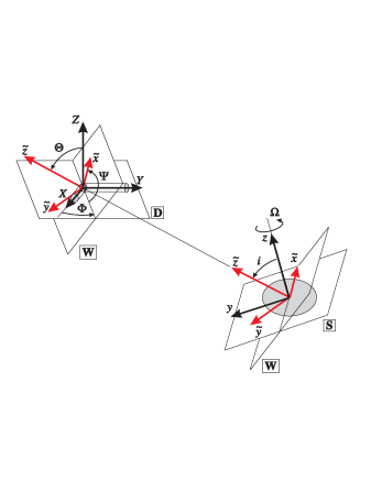
Fig. 7.: Relative orientation of various orthonormal frames introduced in the text: $({\bf e}_{x},{\bf e}_{y},{\bf e}_{z})$ is the neutron star inertial (non-rotating) frame, associated with the ACMC coordinates $(x,y,z)$; $({\bf e}_{x},{\bf e}_{y})$ define the plane S perpendicular to the rotation axis. $({\bf e}_{\tilde{x}},{\bf e}_{\tilde{y}},{\bf e}_{\tilde{z}})$ is the frame associated with the gravitational wave received on Earth; $({\bf e}_{\tilde{x}},{\bf e}_{\tilde{y}})$ define the wave plane W. Note that ${\bf e}_{\tilde{x}}={\bf e}_{x}$. $({\bf e}_{X},{\bf e}_{Y},{\bf e}_{Z})$ is the interferometric detector frame; $({\bf e}_{X},{\bf e}_{Y})$ define the detector plane D.

5 Signal received by an interferometric detector

Due to the weakness of the expected gravitational signal from pulsars, long integration times, typically of the order of the year, are required to extract the signal out of the noise. For such a long observing time, the motion of the Earth must be taken into account for it modifies the position of the pulsar with respect to the antenna pattern of the interferometric detector. It results in a modulation of both the amplitude and the frequency of the signal (Jotania, Valluri & Dhurandhar 1995). Note that if one is searching for a known pulsar, the frequency modulation (Doppler shift) can be obtained readily from the radio observations.

In this section, we examine the daily modulation of the signal amplitude due to the Earth’s rotation. The special case of an interferometric detector situated on the equator with arms symmetrically placed about the North-South direction and a gravitational wave coming from the Northern celestial pole has been treated by Jotania et al. (1995).

5.1 Beam-pattern factors

Let $({\bf e}_{\tilde{x}},{\bf e}_{\tilde{y}},{\bf e}_{\tilde{z}})$ be the orthonormal frame associated with the gravitational wave: ${\bf e}_{\tilde{z}}$ is perpendicular to the wave plane and parallel to the “line of sight”, being orientated from the neutron star centre to the Earth centre; ${\bf e}_{\tilde{x}}$ is the unit vector of the wave plane which is perpendicular to the star’s rotation axis. In the $({\bf e}_{\tilde{x}},{\bf e}_{\tilde{y}},{\bf e}_{\tilde{z}})$ frame the transverse traceless gravitational wave is expressible from its two polarization modes $h_{+}$ and $h_{\times}$ as given by Eqs.(40)-(41) or (58)-(59):

$${\bf h}=h_{+}\,({\bf e}_{\tilde{x}}\otimes{\bf e}_{\tilde{x}}-{\bf e}_{\tilde{y}}\otimes{\bf e}_{\tilde{y}})+h_{\times}\,({\bf e}_{\tilde{x}}\otimes{\bf e}_{\tilde{y}}+{\bf e}_{\tilde{y}}\otimes{\bf e}_{\tilde{x}})\ .$$ (66)

The response of an interferometric detector of the VIRGO/LIGO type to the above gravitational wave depends upon the relative orientation of wave frame with respect to the detector’s arms. Let $({\bf e}_{X},{\bf e}_{Y},{\bf e}_{Z})$ be the orthonormal frame such that ${\bf e}_{Z}$ is perpendicular to the detector plane, pointing toward the zenith and ${\bf e}_{X}$ and ${\bf e}_{Y}$ are unit vectors along the two detector’s arms. Let $(\Theta,\Phi,\Psi)$ be the three Euler angles which specify the position of the wave frame $({\bf e}_{\tilde{x}},{\bf e}_{\tilde{y}},{\bf e}_{\tilde{z}})$ with respect to the detector frame $({\bf e}_{X},{\bf e}_{Y},{\bf e}_{Z})$ (cf. Fig.7). The signal measured by the detector is

$$h(t)=F_{+}(\Theta,\Phi,\Psi)\,h_{+}(t)+F_{\times}(\Theta,\Phi,\Psi)\,h_{\times}(t)\ ,$$ (67)

with the following beam-pattern factors [cf. e.g. Eqs.(103)-(104) of Thorne (1987) or Eq.(7a) of Dhurandhar & Tinto (1988)] :

$$F_{+}(\Theta,\Phi,\Psi) = {1\over 2}(1+\cos^{2}\Theta)\cos 2\Phi\cos 2\Psi$$ (68)

$$\qquad-\cos\Theta\sin 2\Phi\sin 2\Psi$$

$$F_{\times}(\Theta,\Phi,\Psi) = {1\over 2}(1+\cos^{2}\Theta)\cos 2\Phi\sin 2\Psi$$ (69)

$$\qquad+\cos\Theta\sin 2\Phi\cos 2\Psi\ .$$

The Euler angles $(\Theta,\Phi,\Psi)$ are not constant because of the motion of the detector with respect to the source induced by the Earth’s diurnal rotation and revolution around the Sun. To compute their variations let us introduce the “celestial sphere frame” $({\bf e}_{X^{\prime}},{\bf e}_{Y^{\prime}},{\bf e}_{Z^{\prime}})$ such that ${\bf e}_{Z^{\prime}}$ is along the Earth’s rotation axis, pointing toward the North pole, ${\bf e}_{X^{\prime}}$ and ${\bf e}_{Y^{\prime}}$ are in the Earth’s equatorial plane, ${\bf e}_{X^{\prime}}$ pointing toward the vernal point (i.e. ${\bf e}_{X^{\prime}}$ is along the intersection of the Earth’s equatorial plane with the Earth’s orbital plane). For time scales of the order of the year, $({\bf e}_{X^{\prime}},{\bf e}_{Y^{\prime}},{\bf e}_{Z^{\prime}})$ can be considered as fixed with respect to the (approximatively) inertial frame containing the solar system barycentre and the neutron star centre. The wave frame $({\bf e}_{\tilde{x}},{\bf e}_{\tilde{y}},{\bf e}_{\tilde{z}})$ is also fixed with respect to this inertial frame. Then let $(\Theta^{\prime},\Phi^{\prime},\psi)$ be the Euler angles which specify the position of the wave frame with respect to the celestial sphere frame (cf. Fig.8). $\Theta^{\prime}$ and $\Phi^{\prime}$ are simply related to the equatorial coordinates of the neutron star on the celestial sphere (the right ascension ${\bar{\alpha}}$ and the declination ${\bar{\delta}}$) by (cf. Fig.8):

$$\Theta^{\prime}={\bar{\delta}}+{\pi\over 2}\qquad\mbox{and}\qquad\Phi^{\prime}={\bar{\alpha}}-{\pi\over 2}\ .$$ (70)

The triad $({\bf e}_{\tilde{x}},{\bf e}_{\tilde{y}},{\bf e}_{\tilde{z}})$ is related to the triad $({\bf e}_{X^{\prime}},{\bf e}_{Y^{\prime}},{\bf e}_{Z^{\prime}})$ by

$${\bf e}_{\tilde{i}}=A_{\tilde{i}J^{\prime}}\ {\bf e}_{J^{\prime}}\ ,$$ (71)

with the orthogonal matrix [cf. e.g. Eq.(4-46) of Goldstein (1980) with the substitution (70)]

$$A_{\tilde{i}J^{\prime}}\!\!\! =\left(\begin{array}[]{c}\sin{\bar{\alpha}}\cos\psi-\cos{\bar{\alpha}}\sin{\bar{\delta}}\sin\psi\\ -\sin{\bar{\alpha}}\sin\psi-\cos{\bar{\alpha}}\sin{\bar{\delta}}\cos\psi\\ -\cos{\bar{\alpha}}\cos{\bar{\delta}}\end{array}\right.$$ (79)

$$\left.\begin{array}[]{cc}-\cos{\bar{\alpha}}\cos\psi-\sin{\bar{\alpha}}\sin{\bar{\delta}}\sin\psi&\cos{\bar{\delta}}\sin\psi\\ \cos{\bar{\alpha}}\sin\psi-\sin{\bar{\alpha}}\sin{\bar{\delta}}\cos\psi&\cos{\bar{\delta}}\cos\psi\\ -\sin{\bar{\alpha}}\cos{\bar{\delta}}&-\sin{\bar{\delta}}\end{array}\right).$$

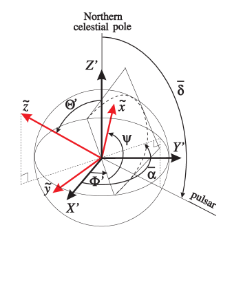
Fig. 8.: Relative orientation of the gravitational wave frame $({\bf e}_{\tilde{x}},{\bf e}_{\tilde{y}},{\bf e}_{\tilde{z}})$ and the celestial sphere frame $({\bf e}_{X^{\prime}},{\bf e}_{Y^{\prime}},{\bf e}_{Z^{\prime}})$.

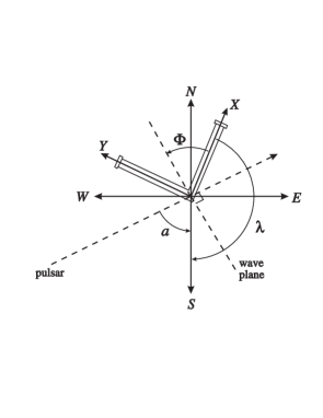
Fig. 9.: Orientation of the detector arms with respect to the local North-South and West-East directions. The dashed line is the projection of the gravitational wave propagation direction on the horizontal plane. The depicted configuration corresponds to that of the VIRGO detector ($\lambda=-161^{o}\,33^{\prime}$).

Let $({\bf e}_{X^{\prime\prime}},{\bf e}_{Y^{\prime\prime}},{\bf e}_{Z^{\prime\prime}})$ be the orthonormal frame linked to the geographical location of the detector site, such that ${\bf e}_{Z^{\prime\prime}}={\bf e}_{Z}$ is the local vertical, ${\bf e}_{X^{\prime\prime}}$ is in the North-South direction and ${\bf e}_{Y^{\prime\prime}}$ is in the West-East direction (cf. Fig.9). The position of the wave frame $({\bf e}_{\tilde{x}},{\bf e}_{\tilde{y}},{\bf e}_{\tilde{z}})$ with respect to the cardinal frame $({\bf e}_{X^{\prime\prime}},{\bf e}_{Y^{\prime\prime}},{\bf e}_{Z^{\prime\prime}})$ is determined by the three Euler angles $(\Theta,\Phi^{\prime\prime},\Psi)$ where $\Theta$ and $\Psi$ are the same angles as those relative to the detector frame and entering Eqs.(68)-(69). The angle $\Phi^{\prime\prime}$ is related to $\Phi$ by

$$\Phi=\Phi^{\prime\prime}+\lambda\ ,$$ (80)

where $\lambda$ is the azimuth of the $X$-arm of the detector, i.e. the angle between the South direction and the $X$-arm, as measured in the retrograd way. $\Phi^{\prime\prime}$ is directly related to the azimuth $a$ of the source by

$$\Phi^{\prime\prime}=-a-{\pi\over 2}\ .$$ (81)

The minus sign which occurs in this relation comes from the fact that the azimuth is measured westwards from the South, hence in the inverse trigronometric way. Putting together relations (80) and (81) we obtain

$$\Phi=-a+\lambda-{\pi\over 2}\ .$$ (82)

Let $(\theta^{\prime\prime},\varphi^{\prime\prime},\psi^{\prime\prime})$ be the Euler angles which specify the position of the cardinal frame $({\bf e}_{X^{\prime\prime}},{\bf e}_{Y^{\prime\prime}},{\bf e}_{Z^{\prime\prime}})$ with respect to the celestial sphere frame $({\bf e}_{X^{\prime}},{\bf e}_{Y^{\prime}},{\bf e}_{Z^{\prime}})$. One has immediatly $\psi^{\prime\prime}=-\pi/2$ because ${\bf e}_{X^{\prime\prime}}$ is orientated in the North-South direction. $\theta^{\prime\prime}$ is simply related to the latitude $l$ of the detector site by

$$\theta^{\prime\prime}={\pi\over 2}-l\ .$$ (83)

$\varphi^{\prime\prime}$ is linked to the local sidereal time $T$ (i.e. the angle between the local meridian and the vernal point) by

$$\varphi^{\prime\prime}=T+{\pi\over 2}\ .$$ (84)

$T$ can be expressed in terms of the sidereal time at Greenwich at 0h UT, $T_{\rm Green}(0)$, and the local UT time $t$ by

$$T(t)=\sigma t+T_{\rm Green}(0)-L\ ,$$ (85)

where $\sigma=1.00273790935\times 15^{o}/{\rm h}$ (Meeus 1991) is a conversion factor from mean solar time to sidereal time (hence $\sigma$ accounts for the revolution of the Earth around the Sun) and $L$ is the longitude of the detector site (the minus sign in front of $L$ comes from the fact that the geographical longitudes are measured positively westwards). The triad $({\bf e}_{X^{\prime\prime}},{\bf e}_{Y^{\prime\prime}},{\bf e}_{Z^{\prime\prime}})$ is related to the triad $({\bf e}_{X^{\prime}},{\bf e}_{Y^{\prime}},{\bf e}_{Z^{\prime}})$ by

$${\bf e}_{I^{\prime\prime}}=B_{I^{\prime\prime}J^{\prime}}\ {\bf e}_{J^{\prime}}\ ,$$ (86)

with the orthogonal matrix

$$B_{I^{\prime\prime}J^{\prime}}=\left(\begin{array}[]{ccc}\sin l\cos T&\sin l\sin T&-\cos l\\ -\sin T&\cos T&0\\ \cos l\cos T&\cos l\sin T&\sin l\end{array}\right)\ .$$ (87)

Now the wave frame $({\bf e}_{\tilde{x}},{\bf e}_{\tilde{y}},{\bf e}_{\tilde{z}})$ is related to the triad $({\bf e}_{X^{\prime\prime}},{\bf e}_{Y^{\prime\prime}},{\bf e}_{Z^{\prime\prime}})$ by

$${\bf e}_{\tilde{i}}=C_{\tilde{i}J^{\prime\prime}}\ {\bf e}_{J^{\prime\prime}}\ ,$$ (88)

with the orthogonal matrix

$$C_{\tilde{i}J^{\prime\prime}}\!\!\! =\left(\begin{array}[]{c}\cos\Psi\cos\Phi^{\prime\prime}-\cos\Theta\sin\Phi^{\prime\prime}\sin\Psi\\ -\sin\Psi\cos\Phi^{\prime\prime}-\cos\Theta\sin\Phi^{\prime\prime}\cos\Psi\\ \sin\Theta\sin\Phi^{\prime\prime}\end{array}\right.$$ (96)

$$\left.\begin{array}[]{cc}\cos\Psi\sin\Phi^{\prime\prime}+\cos\Theta\cos\Phi^{\prime\prime}\sin\Psi&\sin\Psi\sin\Theta\\ -\sin\Psi\sin\Phi^{\prime\prime}+\cos\Theta\cos\Phi^{\prime\prime}\cos\Psi&\cos\Psi\sin\Theta\\ -\sin\Theta\cos\Phi^{\prime\prime}&\cos\Theta\end{array}\right).$$

From equations(71), (86) and (88), the matrix $C$ is given by the product

$$C=A\cdot{}^{t}B\ .$$ (97)

Performing the right-hand-side product and identifying each matrix element by those of expression (96) leads to the following trigonometrical relations

$$\cos\Theta=-\cos{\bar{\delta}}\cos l\cos H(t)-\sin{\bar{\delta}}\sin l$$ (98)

$$\sin\Theta\cos a=\cos{\bar{\delta}}\sin l\cos H(t)-\sin{\bar{\delta}}\cos l$$ (99)

$$\sin\Theta\sin a=\cos{\bar{\delta}}\sin H(t)$$ (100)

$$\sin\Theta\sin\Psi=-\cos\psi\cos l\sin H(t)$$

$$\qquad-\sin\psi\sin{\bar{\delta}}\cos l\cos H(t)+\sin\psi\cos{\bar{\delta}}\sin l$$ (101)

$$\sin\Theta\cos\Psi=\cos\psi\cos{\bar{\delta}}\sin l$$

$$\qquad+\sin\psi\cos l\sin H(t)-\cos\psi\sin{\bar{\delta}}\cos l\cos H(t),$$ (102)

where we have used the relation (81) between $\Phi^{\prime\prime}$ and $a$ and have introduced the local hour angle of the source:

$$H(t)=T(t)-{\bar{\alpha}}=\sigma t+T_{\rm Green}(0)-L-{\bar{\alpha}}\ .$$ (103)

From the above relations the beam-pattern factors $F_{+}(\Theta,\Phi,\Psi)$ and $F_{\times}(\Theta,\Phi,\Psi)$ can be computed for any instant $t$, given the position $(l,L)$ of the detector on the Earth, its orientation $\lambda$, and the position $({\bar{\alpha}},{\bar{\delta}})$ of the source on the sky, as well as the angle $\psi$ that the vector ${\bf e}_{\tilde{x}}$ forms with the intersection line of the wave plane and the Earth’s equatorial plane. First one computes the local hour angle $H(t)$ by Eq.(103), and the angle $\Theta$ by Eq.(98). The angle $\Phi$ is computed by means of Eqs.(82), (99) and (100). Finally, the local polarization angle $\Psi$ is deduced from Eqs.(101) and (102).

Fig. 10.: Relative amplitude of the signal at the frequency $\Omega$ ($A_{1}$, top) and $2\Omega$ ($A_{2}$, bottom) as a function of the local UT time $t$ (assuming a vanishing local sidereal time at 0 h UT), for the specific case of the VIRGO detector and the Crab pulsar. The polarization angle is $\psi=0^{o}$. Each plot corresponds to a given value of the inclination angle $i$. Various lines in the same plot correspond to various values for the angle $\alpha$ between the magnetic axis and the rotation axis: solid line: $\alpha=15.00^{o}$, dashed line: $\alpha=33.75^{o}$, dot-dash-dot-dash line: $\alpha=52.50^{o}$, dotted line: $\alpha=71.25^{o}$, dash-dot-dot-dot line: $\alpha=90.00^{o}$. $\tilde{h}_{0}$ is defined by Eq.(110).

Fig. 11.: Same as Fig.10 but for the polarization angle $\psi=30^{o}$.

Fig. 12.: Same as Fig.10 but for the polarization angle $\psi=60^{o}$. The case $\psi=90^{o}$ is identical to $\psi=0^{o}$ (Fig.10).

5.2 Signal from a rotating magnetized neutron star

According to Eqs.(58)-(59), the gravitational wave signal from a rotating neutron star slightly deformed by its magnetic field is

$$h_{+}(t) = h_{+1}\cos\Omega(t-t_{0})+h_{+2}\cos 2\Omega(t-t_{0})$$ (104)

$$h_{\times}(t) = h_{\times 1}\sin\Omega(t-t_{0})+h_{\times 2}\sin 2\Omega(t-t_{0})\ ,$$ (105)

with

$$h_{+1} = \tilde{h}_{0}{\sin i\cos i\over 2\tan\alpha}$$ (106)

$$h_{+2} = -\tilde{h}_{0}(1+\cos^{2}i)/2$$ (107)

$$h_{\times 1} = \tilde{h}_{0}{\sin i\over 2\tan\alpha}$$ (108)

$$h_{\times 2} = -\tilde{h}_{0}\cos i$$ (109)

$$\tilde{h}_{0} := 6\beta{R^{2}\over cr}{\dot{P}\over P}$$ (110)

Note that in Eqs.(104)-(105) $t_{0}$ accounts for a different time origin between the neutron star frame (where Eqs.(58)-(59) have been derived) and the detector frame. Formally $t_{0}$ accounts also for the propagation delay $r/c$.

According to the above formulæ, when the location $({\bar{\alpha}},{\bar{\delta}})$ of the source is known, the signal $h(t)$ measured by the detector depends on four a priori unknown parameters:

• the inclination angle $i$ of the line of sight with respect to the rotation axis of the star;

• the angle $\alpha$ between the magnetic axis and the rotation axis;

• the polarization angle $\psi$ (cf. Figs.7 and 8) : $\psi$ measures the orientation of the major axis of the ellipse formed by the projection of the neutron star’s equator on the plane of the sky;

• the time $t_{0}$ such that $t_{0}-r/c$ is the instant when the magnetic dipole moment vector $\cal M$ is in the plane formed by the rotation axis and the line of sight, and when the scalar product $\mbox{\boldmath$\cal M$}\cdot{\bf e}_{\tilde{z}}$ is positive.

The signal measured by the detector can be written with the explicit dependence upon these parameters:

$$h(t) = F_{+}\left({t\over t_{\rm SD}},\psi\right)\,h_{+1}(i,\alpha)\cos\Omega(t-t_{0})$$ (111)

$$+F_{\times}\left({t\over t_{\rm SD}},\psi\right)\,h_{\times 1}(i,\alpha)\sin\Omega(t-t_{0})$$

$$+F_{+}\left({t\over t_{\rm SD}},\psi\right)\,h_{+2}(i)\cos 2\Omega(t-t_{0})$$

$$+F_{\times}\left({t\over t_{\rm SD}},\psi\right)\,h_{\times 2}(i)\sin 2\Omega(t-t_{0})$$

where $t_{\rm SD}$ is the duration of one sidereal day: $F_{+}$ and $F_{\times}$ are periodic functions of $t/t_{\rm SD}$, with period one.

Let us introduce the amplitudes of the signal at the frequencies $\Omega$ and $2\Omega$ respectively:

$$A_{1} := \sqrt{F_{+}^{2}\,h_{+1}^{2}+F_{\times}^{2}\,h_{\times 1}^{2}}$$ (112)

$$A_{2} := \sqrt{F_{+}^{2}\,h_{+2}^{2}+F_{\times}^{2}\,h_{\times 2}^{2}}$$ (113)

The daily variation of $A_{1}$ and $A_{2}$, computed from Eqs.(68)-(69) and (98)-(103), is represented in Figs.10-12 for the specific case of the VIRGO detector [$L=-10^{o}\,30^{\prime}$, $l=+43^{o}\,40^{\prime}$ and $\lambda=-161^{0}\,33^{\prime}$ (P.Hello, private communication)] and the Crab pulsar (${\bar{\alpha}}=5\,{\rm h}\,34\,{\rm min}$, ${\bar{\delta}}=+22^{o}\,01^{\prime}$). Note that generally the amplitude of the signal at both $\Omega$ and $2\Omega$ is maximum within a few hours of the instant when the Crab pulsar crosses the local meridian (local sidereal time $T=5\,{\rm h}\,34\,{\rm min}$). Figs.10-12 show that the measure of the time-varying amplitude at one of the two frequencies $\Omega$ and $2\Omega$ allows to determine the polarization angle $\psi$ and the inclination angle $i$. If the signal is recorded at both frequencies, the angle $\alpha$ between the magnetic axis and the rotation axis can be determined as well. Note that this angle is a fundamental parameter for the theory of pulsar magnetospheres.

6 Conclusion

We have considered the gravitational radiation emitted by a distorted rotating fluid star. The distortion is supposed to be symmetric with respect to some axis which does not coincide with the rotation axis. The gravitational emission takes place at two frequencies: $\Omega$ and $2\Omega$, where $\Omega$ is the rotation frequency, except in the particular case where the distortion axis is perpendicular to the rotation axis (only the frequency $2\Omega$ is then present). As an application, the magnetic field induced deformation is treated. If, as usually admitted, the period derivative, $\dot{P}$, of pulsars is a measure of their magnetic dipole moment, the gravitational wave amplitude can be related to the observable parameters $P$ and $\dot{P}$ of the pulsars and to a factor $\beta$ which measures the distortion response of the star to a given magnetic dipole moment. $\beta$ depends on the nuclear matter equation of state and on the magnetic field distribution. The amplitude at the frequency $2\Omega$, expressed in terms of $P$, $\dot{P}$ and $\beta$, is independent of the angle $\alpha$ between the magnetic axis and the rotation axis, whereas at the frequency $\Omega$, the amplitude increases as $\alpha$ decreases.

Using a numerical code generating self-consistent models of magnetized neutron stars within general relativity, we have computed the deformation for explicit models of the magnetic field distribution and a realistic equation of state. It appeared that the distortion at fixed magnetic dipole moment depends very sensitively on the magnetic configuration. The case of a perfect conductor interior with toroidal electric currents is the less favorable one, even if the currents are concentrated in the crust. Stochastic magnetic fields (that we modeled by considering counter-rotating currents) enhance the deformation by several orders of magnitude and may lead to a detectable amplitude for a pulsar like the Crab. As concerns superconducting interiors — the most realistic configuration for neutron stars — we have studied numerically type I superconductors, with a simple magnetic structure outside the superconducting region. The distortion factor is then $\sim 10^{2}$ to $10^{3}$ higher than in the normal (perfect conductor) case, but still insufficient to lead to a positive detection by the first generation of kilometric interferometric detectors. We have not studied in details the type II superconductor but have put forward some argument which makes it a promising candidate for gravitational wave detection. Due to the complicated microphysics involved in type II superconductors we delay their study to a future paper. We also plan to study the deformation induced by a possible ferromagnetic solid interior of neutron stars, as well as the effects of a strong toroidal internal magnetic field.

Regarding the reception of gravitational waves from a pulsar by an interferometric detector, we have computed the amplitude modulation of the signal induced by the diurnal rotation of the Earth. By inspecting the wave form, and assuming the position of the pulsar to be known (the pulsar can be recognized by its period), one can determine the inclination angle of the line of sight with respect to the pulsar rotation axis, as well as the orientation of the pulsar equatorial plane. Moreoever, by comparing the wave forms at the frequencies $\Omega$ and $2\Omega$, the angle $\alpha$ between the rotation axis and the magnetic axis can be determined.

Pulsars may be good candidates for the detection by the forthcoming VIRGO and LIGO interferometric detectors. A frequently invoked mechanism for gravitational emission concerns asymmetries of the neutron star solid crust and the resulting precession. In this article, we have examined instead the bulk deformation of the star induced by its own magnetic field. For some configurations of the magnetic field (stochastic distribution, type II superconductor), the deformation may be large enough to lead to a detectable signal by VIRGO, with the total magnetic dipole moment (or equivalently the surface magnetic field) keeping its (relatively small) observed value. The positive detection of gravitational waves from pulsars would lead to some constraints on the internal magnetic field distribution, which would be of great interest for the theories of pulsar magnetospheres. This would constitute an example of a significant contribution of gravitational astronomy to classical astrophysics.

• We warmly thank François Bondu and Patrice Hello for useful discussions and for checking the calculations presented in Sect.5. We are also indebted to Sreeram Valluri for his careful reading of the manuscript. The numerical calculations have been performed on Silicon Graphics workstations purchased thanks to the support of the SPM department of the CNRS and the Institut National des Sciences de l’Univers.

A From QI to ACMC coordinates

Most studies of stationary rotating neutron stars make use of quasi-isotropic (QI) coordinates $(t,r^{\prime},\theta^{\prime},\varphi)$ (cf. the discussion in Sect.2 of Bonazzola et al. 1993). In these coordinates, the spatial components of the metric tensor have the following asymptotic behavior:

$$g_{r^{\prime}r^{\prime}} = 1+{\alpha_{1}\over r^{\prime}}+{\beta_{11}\cos 2\theta^{\prime}+\beta_{10}\over{r^{\prime}}^{2}}+O\left({1\over{r^{\prime}}^{3}}\right)$$ (A1)

$$g_{\theta^{\prime}\theta^{\prime}} = \left[1+{\alpha_{1}\over r^{\prime}}+{\beta_{11}\cos 2\theta^{\prime}+\beta_{10}\over{r^{\prime}}^{2}}+O\left({1\over{r^{\prime}}^{3}}\right)\right]{r^{\prime}}^{2}$$ (A2)

$$g_{\varphi\varphi} = \left[1+{\alpha_{3}\over r^{\prime}}+{\beta_{30}\over{r^{\prime}}^{2}}+O\left({1\over{r^{\prime}}^{3}}\right)\right]{r^{\prime}}^{2}\sin^{2}\theta^{\prime}\ ,$$ (A3)

where $\alpha_{1}$, $\alpha_{3}$, $\beta_{10}$, $\beta_{11}$ and $\beta_{30}$ are some constants. By comparison with the definition (4), it appears that such coordinates are not ACMC to order 1: in order to be so, the $1/{r^{\prime}}^{2}$ term in $g_{r^{\prime}r^{\prime}}$ and $g_{\theta^{\prime}\theta^{\prime}}$ should not contain any $\cos 2\theta^{\prime}$, i.e. $\beta_{11}$ should vanish. It can be seen easily that the following coordinate transformation leads to an ACMC coordinate system $(t,r,\theta,\varphi)$:

$$r^{\prime} = r+{\beta_{11}\cos^{2}\theta\over r}$$ (A4)

$$\theta^{\prime} = \theta-{\beta_{11}\cos\theta\,\sin\theta\over r^{2}}\ .$$ (A5)

By computing the $g_{00}$ component in the $(t,r,\theta,\varphi)$ coordinates from the components $g_{\alpha^{\prime}\beta^{\prime}}$ in the $(t,r^{\prime},\theta^{\prime},\varphi)$ coordinates and by identification with Eq.(2), one obtains the following value of Thorne’s mass quadrupole moment:

$${\cal I}_{xx} = {\cal I}_{yy}=-{1\over 2}{\cal I}_{zz}$$ (A6)

$${\cal I}_{zz} = {4\over 9}\left(\gamma_{2}-M\beta_{11}\right)$$ (A7)

$${\cal I}_{ij} = 0\quad\mbox{if}\quad i\not=j\ ,$$ (A8)

where (i) $\gamma_{2}$ is the coefficient of $\cos 2\theta^{\prime}$ in the $1/{r^{\prime}}^{3}$ term of the $1/r^{\prime}$ expansion of the metric component $g_{00}$ in the QI coordinates $(t,r^{\prime},\theta^{\prime},\varphi)$ and (ii) $M$ is half the coefficient of $1/r^{\prime}$ in the same expansion ($M$ is nothing else than the total gravitational mass of the star).

To summarize, Thorne’s quadrupole moment component ${\cal I}_{zz}$ can be computed via equation (A7) by reading off the coefficients $\beta_{11}$ and $\gamma_{2}$ in the $1/r^{\prime}$ expansions of the metric components in the QI coordinates.

References

- 1 Alpar M.A., Pines D., 1985, Nature 314, 334
- 2 Arnett W.D., Bowers R.L., 1977, ApJS 33, 415
- 3 Barone F., Milano L., Pinto I., Russo G., 1988, A&A 203, 322
- 4 Bocquet M., Bonazzola S., Gourgoulhon E., Novak J., 1995, A&A 301, 757
- 5 Bonazzola S., Frieben J., Gourgoulhon E., 1996, ApJ 459 (March 10, 1996), in press (preprint: gr-qc/9509023)
- 6 Bonazzola S., Gourgoulhon E., Salgado M., Marck J.A., 1993, A&A 278, 421
- 7 Bonazzola S., Marck J.A., 1994, Annu. Rev. Nucl. Part. Sci. 45, 655
- 8 Bondu F., 1996, PhD Thesis, Université Paris XI
- 9 Chandrasekhar S., 1969, Ellipsoidal figures of equilibrium. Yale University Press, New Haven
- 10 de Araújo J.C.N., de Freitas Pacheco J.A., Horvath J.E., Cattani M., 1994, MNRAS 271, L31
- 11 Dhurandhar S.V., Tinto M., 1988, MNRAS 234, 663
- 12 Gal’tsov D.V., Tsvetkov V.P., Tsirulev A.N., 1984, Zh. Eksp. Teor. Fiz. 86, 809; English translation in Sov. Phys. JETP 59, 472
- 13 Gal’tsov D.V., Tsvetkov V.P., 1984, Phys. Lett. 103A, 193
- 14 Goldreich P., 1970, ApJ 160, L11
- 15 Goldstein H., 1980, Classical Mechanics, 2nd edition. Addison-Wesley, Reading, MA
- 16 Haensel P., 1995, in Physical processes in astrophysics, Lecture notes in physics 458, eds. I.W.Roxburgh, J.L.Masnou. Springer-Verlag, Berlin
- 17 Ipser J.R., 1971, ApJ 166, 175
- 18 Jotania K., Valluri S.R., Dhurandhar S.V., 1995, A&A, in press
- 19 Lorenz C.P., Ravenhall D.G., Pethick C.J., 1993, Phys. Rev. Lett. 70, 379
- 20 Lyne A.G., Manchester R.N., 1988, MNRAS 234, 477
- 21 Manchester R.N., Taylor J.H., 1977, Pulsars. Freeman, San Francisco
- 22 Meeus J., 1991, Astronomical algorithms. Willmann-Bell
- 23 Muslimov A., Page D., 1996, ApJ 458, 347
- 24 Misner C.W., Thorne K.S., Wheeler J.A., 1973, Gravitation. Freeman, New York
- 25 New K.C.B., Chanmugam G., Johnson W.W., Tohline J.E., 1995, ApJ 450, 757
- 26 Pines D., Shaham J., 1974, Comments Astrophys. 6, 37
- 27 Rankin J.M., 1990, ApJ 352, 247
- 28 Ruderman M., 1991, ApJ 382, 576
- 29 Ruderman M., 1994, in Cosmical magnetism, ed. D.Lynden-Bell. Kluwer Academic Publishers
- 30 Salgado M., Bonazzola S., Gourgoulhon E., Haensel P., 1994, A&A 291, 155
- 31 Schutz B.F., 1987, in Gravitation in astrophysics, eds. B. Carter & J.B. Hartle. Plenum Press, New York
- 32 Shapiro S.L., Teukolsky S.A., 1983, Black holes, white dwarfs and neutron stars. John Wiley, New York
- 33 Straumann N., 1984, General relativity and relativistic astrophysics. Springer Verlag, Berlin
- 34 Taylor J.H., Manchester R.N., Lyne A.G., 1993, ApJS 88, 529
- 35 Taylor J.H., Manchester R.N., Lyne A.G., Camilo F., 1995, unpublished work
- 36 Thompson C., Duncan R.C., 1993, ApJ 408, 194
- 37 Thorne K.S., 1980, Rev. Mod. Phys. 52, 299
- 38 Thorne K.S., 1987, in 300 years of gravitation, eds. S.Hawking, W.Israel. Cambridge University Press, Cambridge
- 39 Thorne K.S., Gürsel Y., 1983, MNRAS 205, 809
- 40 Wald R.M., 1984, General relativity. University Chicago Press, Chicago
- 41 Wiringa R.B., Fiks V., Fabrocini A., 1988, Phys. Rev. C 38, 1010
- 42 Zimmermann M., 1978, Nature 271, 524
- 43 Zimmermann M., 1980, Phys. Rev. D 21, 891
- 44 Zimmermann M., Szedenits E., 1979, Phys. Rev. D 20, 351