The lightcurve reconstruction method for measuring the time delay of gravitational lens systems
Bernhard Geiger & Peter Schneider
Max-Planck-Institut für Astrophysik
Karl-Schwarzschild-Str. 1, Postfach 1523
D-85740 Garching bei München, Germany
Abstract: We propose a new technique to measure the time delay of radio-loud gravitational lens systems, which does not rely on the excessive use of interferometric observations. Instead, the method is based on single-dish flux density monitoring of the (unresolved) lens system’s total lightcurve, combined with additional interferometric measurements of the flux density ratio at a few epochs during that monitoring period.
The basic idea of the method is to reconstruct the individual image lightcurves from the observed total lightcurve by assuming a range of potential values for the time delay and the magnification ratio of the images. It is then possible to single out the correct reconstruction, and therefore determine the time delay, by checking the consistency of the reconstructed individual lightcurves with the additional interferometric observations. We performed extensive numerical simulations of synthetic lightcurves to investigate the dependence of the performance of this method on various parameters which are involved in the problem. Probably the most promising candidates for applying the method (and also for determining the Hubble constant) are lens systems consisting of multiply imaged compact sources and an Einstein ring, such as B0218+357 from which some of the parameters used for our simulations were adopted.
1 Introduction
Already many years ago it was realised (Refsdal 1964) that gravitational lensing provides a way to determine the Hubble constant. This method is based on measuring the time delay between the arrival times of light rays corresponding to different images in gravitational lens systems. Of course, an intrinsic variation of the source on appropriate timescales is essential for the time delay to be detectable. In addition, the redshifts of source and deflector and a reliable model for the mass distribution of the deflector are required to calculate the Hubble constant. The advantage of the time delay method (as also of the Sunyaev-Zel’dovich effect and potentially also of SN Ia) compared to conventional techniques for determining is the possibility to reach cosmological distances directly without using a “distance ladder” of intermediate calibration steps.
The first lens system discovered, the double quasar 0957+561 (Walsh et al. 1979), has been monitored since then at optical and radio frequencies, and quite a number of papers about its time delay have been published. However, the value of still remains controversial today, because these studies were plagued by problems like unevenly sampled data points and microlensing effects. For an overview of the status quo see Chap. 2 of Kochanek & Hewitt (1996). But even if a secure value for were available, this would not be of much use for determining the Hubble constant, because it is extremely difficult to specify a unique model for the lens mass distribution in this system. This problem arises because not only a single galaxy, but also the cluster of galaxies in which it is located, as well as another cluster at a different redshift, are contributing to the image splitting, and so even in the simplest realistic models there are more parameters than can be constrained observationally (e.g. Kochanek 1991, Bernstein et al. 1993; but also see Grogin & Narayan 1996).
A very much better candidate for determining is the lens system B0218+357 (Patnaik et al. 1993), consisting of two images of a compact flat spectrum radio source and an Einstein ring of extended emission. This system combines several important advantages. The small image separation of implies that probably a single galaxy is acting as a lens. In addition, the morphology of the compact images (Patnaik et al. 1995) and especially the radio ring provide valuable information about the mass distribution of the lensing galaxy. Thus it should be feasible to construct a sufficiently accurate and well-constrained lens model for this system. Furthermore, as the time delay for this system is expected to be of the order of two weeks, and the source is known to be variable, a determination of should be possible on reasonable timescales of a few months. In fact, Corbett et al. (1996) already published a value of days, derived from the time variation of the image polarization in VLA monitoring observations.
In this paper we are investigating the possibilities for determining the time delay of radio-loud gravitational lens systems without the excessive use of expensive interferometric observations. Instead, we consider monitoring the total flux density of the unresolved lens system with a single-dish radio telescope. As we briefly motivate in Sect. 2 an analysis of the autocorrelation function of the combined lightcurve is a straightforward approach to extract the value of the time delay. However, numerical simulations show that it is difficult to apply this method in practice, because it would require unrealistically long monitoring periods in order to achieve significant results. Therefore the main part of this paper (Sect. 3) is devoted to a new method which is shown to yield a much more reliable result for the time delay by making use of a few additional interferometric measurements. The idea of this method is to reconstruct the lightcurves of the individual images from the observed combined lightcurve by assuming values for the time delay and the magnification ratio of the images. To single out the true value of the time delay we use the consistency of the reconstructed lightcurves with additional information about the flux density ratio of the images at different epochs obtained from interferometric observations. In extensive simulations we investigate the performance of this “lightcurve reconstruction method”, depending on the various parameters involved, and show that typically a handful of interferometric observations suffice to determine reliably. Finally, in Sect. 4 we summarize the results and discuss the prospects for the application of this new method, especially in context with the most promising lens system B0218+357.
The discussion in this paper is restricted to gravitational lens systems with two images of a compact source, although the formalism described here might as well be extended to a larger number of images. As we are mainly interested in radio lightcurves it is justified to neglect microlensing effects for this study. Furthermore we assume that there is no variation on relevant timescales in the flux density of extended emission which may be associated with the compact source (e.g. the ring in B0218+357).
2 Autocorrelation approach
2.1 Time delay effect on the autocorrelation function
The total lightcurve of a two-image gravitational lens system results from a time shifted superposition of the intrinsic source lightcurve and a constant contribution (e.g., from an extended source component) in the following way:
| (1) |
and denote the flux density and the absolute magnification of the individual images.111In the following we will restrict the time delay to be positive. Hence the index denotes the image in which intrinsic source variations will appear first. Introducing the observable magnification ratio and subtracting the time averages of the flux densities, , and , Eq. (1) becomes
| (2) |
Here we assume that is a stationary random process and define its (normalized) autocorrelation function as
It is obvious that the time delay should show up in as a positive contribution to the autocorrelation at . Starting from Eq. (2) it is an easy exercise to show that can be calculated from the intrinsic autocorrelation function of the source according to
| (3) |
with the factor ensuring the proper normalization. Corresponding to the change in the autocorrelation function the power spectrum is modified according to
| (4) |
where denotes the intrinsic power spectrum of the unlensed source.
Figure 1a graphically depicts the modification of the autocorrelation function described by Eq. (3). Here we took the values (in arbitrary time units222By scaling all time variables appropriately the arbitrary time units used here can be adapted to any lens system of interest.) for the time delay, for the magnification ratio and
| (5) |
as an example for the intrinsic autocorrelation function, which corresponds to the reasonable intrinsic power spectrum
| (6) |
The parameter represents a characteristic timescale of the intrinsic source variability and has been chosen to be for this plot. The resulting autocorrelation function shows a distinct maximum at the value of the time delay. Thus it is at least in principle possible to obtain information about by analysing the autocorrelation function of combined lightcurves. However, if the timescale of variability is comparable to or longer than , the “time delay peak” will merge with the “intrinsic maximum” of at and any information on will be lost.

2.2 Analysis of for simulated lightcurves
Of course, in applications to observations the limited observing time , the finite sampling interval and observational errors will impose serious constraints on the usefulness of the autocorrelation function for determining the time delay. To study this quantitatively we used synthetic data sets of combined lightcurves. These lightcurves were generated as realizations of a gaussian random process with the intrinsic power spectrum of Eq. (6). For simplicity we restricted the study to constant observing intervals .
| parameter | symbol | standard value |
|---|---|---|
| observing period | 100 | |
| observing interval | 1 | |
| observing error | 0.1 | |
| power spectrum | ||
| timescale of variability | 3.18 | |
| magnification ratio | 3 | |
| time delay | 20 |
In Fig. 1b the autocorrelation function for one typical lightcurve realization with parameters as summarized in Table 1 is plotted. Due to the limited observing period , which does not provide a “fair sample” of the lightcurve’s statistical properties, a number of additional maxima and minima are now showing up, making it very difficult to identify the time delay peak. A simple quantitative measure for the performance of the autocorrelation method is the fraction of lightcurve realizations for which the time delay maximum, i.e. the maximum closest to the true time delay, is in fact the highest maximum within the range of potential values. In the following all maxima in the range except the =0 maximum are considered. We studied the dependence of (and other measures) on all of the parameters shown in Table 1, but here we only present the results for varying and , keeping the other parameters fixed.

From Fig. 2a it can be seen that prolonging the observation period leads to an increase in , because with increasing the sampling of the lightcurve improves and the observed autocorrelation function converges to the theoretical shown in Fig. 1a. However, since for some realizations the unwanted additional maxima in can be quite stable, it takes a rather long observing time to ensure getting significant results for the time delay. In Fig. 2b the dependence of on the magnification ratio is depicted. Of course the method works best for , as for increasing magnification ratio the combined lightcurve is dominated more and more by the brighter image. The autocorrelation function will then be dominated by the first term in Eq. (3), which does not contain the time delay, and converges to the intrinsic autocorrelation function for .
To summarize, one can say that an analysis of the autocorrelation function of the total lightcurve of gravitational lens systems only constitutes a viable method for determining the time delay if the magnification ratio is close to unity and the observing period is very much longer than and .
3 Lightcurve reconstruction method
In this section we introduce the “lightcurve reconstruction method” for measuring the time delay of gravitational lens systems. As we will explain in Sect. 3.1, it is possible to reconstruct the (unobserved) lightcurves and of the individual images, if we assume values for the time delay and the magnification ratio . Sect. 3.2 shows qualitatively how the true value can then be singled out by checking the consistency of the reconstructed lightcurves with additional information from interferometric measurements about the flux density ratio of the images. In Sect. 3.3 this is discussed quantitatively in terms of the function. Using lightcurve simulations we investigate in Sect. 3.4 the dependence of the results on the various parameters that are involved in this problem. Finally, Sect. 3.5 shows how confidence intervals for the time delay can be obtained in individual realizations.
3.1 Reconstruction of lightcurves
It is convenient to discuss the method by looking at Fig. 3. As an example for an “observed” combined lightcurve Fig. 3a displays one realization of a gaussian random process with parameters as shown in Table 1 except that here we took . Now, to reconstruct the individual image lightcurves and we have to postulate values and for the time delay and the magnification ratio, respectively.333Here and in the following the subscript indicates quantities used for or obtained from the reconstruction. It will become clear in the following subsections how to actually determine these quantities with this method. In the example of Fig. 3 we used just for illustration the values and which in fact agree with the “true” values used for generating the combined lightcurve. In addition, we have to make a guess about the individual lightcurve in the time interval , but luckily the choice for this initial guess will turn out to be rather irrelevant for the method to work. For simplicity we use for within this paper.

Having specified , and for we can immediately calculate the individual lightcurve in the same interval using
| (7) |
which is trivially derived from Eq. (2). The application of Eq. (7) is visualized by a solid arrow in Fig. 3b. The next step is to compute on the subsequent interval using
| (8) |
This is indicated by the dashed arrows of Fig. 3b. By iteratively applying Eqs. (7) and (8), the individual image lightcurves can be reconstructed for the total observing period. Introducing the notation for the restriction of the function to the interval , the reconstruction process can be written as444Note that the quantities in this notation are still meant to be functions of although the argument has been omitted.
| (9) |
and
| (10) |
Now we would like to quantify the rms errors and of the reconstructed individual lightcurves under the hypothesis that the values and used for the reconstruction are in fact the true ones. Therefore these errors include the observational errors of the total lightcurve measurements and the errors caused by the arbitrary initial guess. In the following we assume the observational errors to be normally distributed with standard deviation and statistically independent for each data point. Hence the increase of with respect to when applying Eq. (7) is described by
| (11) |
whereas using Eq. (8) leads to an evolution of the error according to
| (12) |
In analogy to Eqs. (9) and (10) the error propagation during the reconstruction can be compactly expressed as
| (13) |
and
| (14) |
However, looking at Fig. 3c is much more illustrative to understand the evolution of the errors of the reconstructed lightcurves. For the first interval we have to estimate the error caused by the arbitrary initial guess. Here we assume that the variability characteristics of the second lightcurve in the starting interval does not substantially differ from the observed variability of the combined lightcurve during the total observing period. This leads to the estimate with denoting the dispersion of the combined lightcurve during the observation period.555For lightcurves with timescale of variability comparable to (or larger than) the dispersion is increasing when extending the interval on which it is calculated from to . Therefore, the dispersion used for this estimate should be calculated on an interval equal to in such cases, because otherwise the error of the initial guess would be overestimated. Figure 3c clearly shows that the initial uncertainty in the reconstructed lightcurves decreases at every interval, because the errors are multiplied with the factor in Eq. (12). Thus the reconstruction is most accurate at the end of the observing period. Here the errors are dominated by the observational errors of the combined lightcurve, which are added when applying Eq. (11), and the initial uncertainty has almost dropped out. Of course the reconstruction works best for large values of the magnification ratio because then the initial errors are decreasing faster. In the following we will restrict to be larger than one, because otherwise the errors will actually grow and the reconstruction fails. However, this is no fundamental problem for the method, since for , i.e. in cases in which the light arrives first in the weaker image, the reconstruction can be done starting at the end of the observing period.
For simplicity we will assume for this study that the standard deviation of the observational errors of the combined lightcurve is constant for all data points, . In addition, we restrict the simulations performed in this paper to constant observing intervals . It should be emphasized here that the limitation to constant and is merely for convenience, and removing these restrictions does not impose any conceptual difficulties for the reconstruction method. An important point to be mentioned is the following. The errors and shown in Fig. 3c are strictly correct only for integer multiples of the observing interval . In order to calculate the reconstructed lightcurves for values lying between the data points, the observed combined lightcurve has to be interpolated which in general introduces additional errors. Interpolation also is necessary to do the reconstruction with not being an integer multiple of . We use a linear interpolation and determine the error introduced by the interpolation directly from an ensemble of simulated lightcurves. For real data, however, an extrapolation of the variability characteristics to timescales shorter then the sampling interval has to be made in order to get an estimate of the errors introduced by interpolation. In practice this could be achieved by following the approach of Press et al. (1992a). They describe a method that provides a “reconstruction of a set of irregularly sampled measurements into a continuous function and an associated standard error function” by using an estimate of the underlying autocorrelation function obtained from the data.
Figure 4 shows another example for a lightcurve generated according to a gaussian random process666Note that the reconstruction method does not rely on properties like gaussianity or stationarity. The reason to use gaussian random processes for the simulations is just because they are easy to generate. with the parameters of Table 1. In Fig. 4a the unobserved individual image lightcurves and are depicted. With and these add up to the observed combined lightcurve in Fig. 4b. In Fig. 4c the individual lightcurves are reconstructed using the true values for and , whereas Fig. 4d shows the reconstruction using the wrong value for the time delay. In agreement with the error discussion above the correctly reconstructed lightcurves resemble the true ones quite closely towards the end of the observing period. Of course now the problem arises how to distinguish between the correct reconstruction (Fig. 4c) and the wrong one in Fig. 4d as well as all the other wrong reconstructions conceivable with different ’s and ’s. Although it might be possible in some special cases to infer by making assumptions about the shape of correctly reconstructed lightcurves, this is certainly not viable in general. Therefore we clearly need some additional information to solve the problem.

3.2 Flux density ratios as additional constraints
For the rest of this paper we investigate the chances for determining the time delay by using additional observational constraints about the flux density ratio of the images obtained from interferometric observations. It is useful to take the flux density ratio rather than absolute flux densities of the images, because measuring the former does not suffer from calibration problems and is therefore much more accurate.
The time dependent flux density ratio of the two images is given by
| (15) |
where and denote the flux densities without subtraction of the mean values (cf. the definition in Sect. 2). In the final identity of this equation the individual image time averages have been expressed in terms of the combined lightcurve average . Note that only includes the flux densities of the varying components in the lens system. Thus in order to determine at least one interferometric observation is required to subtract the constant flux density of non varying components from the average single-dish flux density.
In analogy to Eq. (15) we can calculate the reconstructed flux density ratio from the reconstructed individual image lightcurves as follows:
| (16) |
In order to express in terms of quantities with independent errors we replaced with in this equation, because for a given epoch the reconstruction error only contains observational errors of for epochs preceding and therefore is independent of . By applying the usual error propagation law we obtain the relation
| (17) | |||||
for the error of the reconstructed flux density ratio under the hypothesis that and are the true values.

The filled circles at and the dotted vertical lines in the top panel indicate additional interferometric flux density ratio measurements.
Figure 5 shows the unobserved true time evolution of the flux density ratio for the example of Fig. 4 as well as its correct and wrong reconstructions , corresponding to the lightcurve reconstructions in Fig. 4c and d. In order to compute the flux density ratio curves for this example we have to specify the value of appearing in Eqs. (15) and (16). To do so we introduce a new parameter for our lightcurve simulations, which is not included in Table 1 because it was not relevant for the autocorrelation analysis. We define the parameter
as the ratio of the total lightcurve’s dispersion to the average combined flux density in order to describe the relative variability of the source. For the example case a variability of has been chosen. The reconstructed flux density ratio curves in Fig. 5 also include error bars calculated from Eq. (17). Again it can be seen that the initial uncertainty gradually decreases during the reconstruction process. At the end of the observing period () the contributions of and to the error of the flux density ratio are comparable, whereas that of is negligible.

From Fig. 5 it is clear that an additional measurement of the flux density ratio, say at , can rule out the combination of the values for the time delay and for the magnification ratio, because these would lead to a completely wrong prediction for the flux density ratio at that epoch. However, we have to test the compatibility of all potential values for and with the additional constraint . This has been done in Fig. 6a. The hatched area in this plot includes all pairs of parameter values (, ) with the reconstructed flux density ratio being compatible with the measured flux density ratio within a error margin, i.e.
The values for the flux density ratio measurements used here and below include a normally distributed observational error with standard deviation . Note that for any time delay there is, at least for this example, a value for the magnification ratio which yields a reconstruction in agreement with the additional flux density ratio constraint. Thus in order to restrict the range of possible time delay values, more than one flux density ratio measurement is required. Figure 6b additionally shows the consistency region defined by another flux density ratio measurement performed at , and in Fig. 6c a third measurement at is included. The intersection of these regions is filled black. These plots nicely illustrate how the method works. However, to quantify the consistency of parameter values (, ) with the interferometric constraints a discussion in terms of is adequate.
3.3 Analysis of minima in the function
In general functions are used to fit parametrized models to a given data set and to quantify the compatibility of the model with the data. In the case discussed here the “model” is represented by the basic assumptions made for this study which were formulated in the last paragraph of the introduction. The postulated values for the time delay and for the magnification ratio can be regarded as the fit parameters. Therefore we define as a function of and :
| (18) |
denotes the number of interferometric flux density ratio measurements. Note that here not only the observational data but also the values predicted by the model contain errors777These errors also depend on the fit parameters and . Strictly speaking, this parameter dependence of the errors leads to an additional term which has to be considered when deriving the function from the maximum likelihood principle. However, this term can be neglected here because the variation of the errors is small for parameter values of interest. which have to be included in the function. Another peculiarity of the used here is the extreme non-linearity of the model in its fit parameter . This leads to the ocurrence of a variety of minima in the function and to non-elliptic confidence regions for the parameter values. However, as we will see below the model is still sufficiently linear locally (at individual minima), so that statistics can be applied (see e.g. Sect. 15.6 of Press et al. 1992b).
Figure 6d shows the contours of the function for the same number of interferometric measurements as in Fig. 6c. The definition of the consistency value for which has been used here will be given below. This plot reveals that the information from the three flux density ratio measurements included here does not suffice to determine the time delay unambiguously. There are still a number of minima left. In the following we will call the minimum which is closest to the true parameter values the true minimum and all other minima will be termed wrong minima. Figure 7 depicts the evolution of the contours when the number of interferometric measurements is further increased. It can be seen here that the wrong minima are gradually vanishing. For the true minimum is the only minimum remaining and therefore a definite time delay determination can be obtained. However, already for the global minimum in the function, which gives the best fit parameter values, corresponds to the true minimum.

| parameter | symbol | standard value |
|---|---|---|
| relative source variability | 2% | |
| number of interferometric observations | 5 | |
| interval between interferometric observations | 5 | |
| error of flux density ratio measurements | 0.5% | |
| error of the average combined flux density | 2% |

To test the lightcurve reconstruction method we again used simulated lightcurves with parameters as shown in Table 1. Additional parameters which have to be specified for the lightcurve reconstruction are displayed in Table 2. This table also shows the “standard values” that we have adopted for these parameters in the simulations. For simplicity the intervals between the interferometric observations are assumed to be constant. These observations are performed towards the end of the observing period when the reconstruction is most accurate. Again we considered all minima in the range as potential time delay values.888In practice, of course, a plausible range of potential time delay values can be given if a lens model is available. For B0218+357, e.g., the time delay is expected to be roughly between 8 and 20 days. Figure 8 summarizes the results of applying the reconstruction to simulated lightcurves with the parameter values of Tables 1 and 2. Figure 8a shows the cumulative distribution of the values at the global minimum of the function. From this plot it can be seen that for most of the simulated lightcurves the location of the global minimum in fact agrees with the value for the time delay which has been used for generating them. To get an estimate of the accuracy achievable for the time delay determination, Fig. 8b depicts the distribution of the values at the true minimum. The narrow distribution centered on the exact value of shows that a fairly high precision can be expected with the standard parameter values used here. However, to obtain error ranges for individual realizations, statistics can be applied. This will be discussed in Sect. 3.5. Plots c and d of Fig. 8 show the distribution of the values at the global and at the true minimum, respectively. For the rather small lightcurve variability of it is not surprising that the magnification ratio is well determined here. The two distributions are nearly identical, because also in the few cases where the global minimum is a wrong minimum, it is located roughly at the correct value for the magnification ratio (cf. Fig. 6d). Figure 8e shows the distribution of the rank of the true minimum when ordering the minima according to rising values. For of the lightcurves the global minimum in the function corresponds to the true minimum, and only for the rank of the true minimum is higher than 2. Finally, Fig. 8f displays the distribution of the number of minima which are appearing in the function. In the majority of cases just one or a few minima are occurring, but there are also rare cases with a large number of minima showing up.

In the following paragraph we will check if some statements given by statistics are applicable for this analysis. Let denote the number of constraints used in a fit and be the number of fit parameters. According to statistics the probability density distribution for the value at the minimum of the function is given by a -distribution with degrees of freedom, i.e.
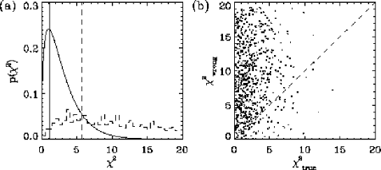
This is valid if the errors are normally distributed and the model is linear in its fit parameters. In our case, however, the model is extremely non-linear in the fit parameter , and as we have mentioned before this leads to the occurrence of additional wrong minima which cannot be described by statistics. As we have seen in Fig. 8e the wrong minima can be lower than the true minima. Therefore the relation given above is certainly not valid any more for the global minimum of the function. Nevertheless the values at the true minima still obey a -distribution with degrees of freedom. This is visualized by the thick, solid-line histogram in Fig. 9 which shows the distribution of the values at the true minimum for the simulated lightcurves and which matches quite well with the overlaid theoretical -distribution with degrees of freedom as it is expected for constraints and fit parameters. In addition, this figure reveals that the distribution of the values at the exact parameter values is consistent with a -distribution with degrees of freedom, again in agreement with the predictions of statistics. The thin, solid-line histogram in Fig. 9 depicts the distribution of the values at the lowest wrong minimum of the function which of course is not described by statistics. The dotted vertical lines in the figure indicate limiting confidence values for rejecting the hypothesis that some given parameter values and are the correct ones. These exclusion confidence values have been derived from the -distribution with degrees of freedom for at the exact parameter values. Corresponding definitions already have been used for the contours in Figs. 6d and 7 and for quantifying the frequency of wrong minima in Fig. 8f. Actually this is a conservative limit for rejecting wrong minima, because for the exclusion of the hypothesis that a given minimum is the true one we would have to use the -distribution with degrees of freedom which is shifted to smaller values. In Sect. 3.5 we will show with an example how to assign significance values to the statement that one of several minima in the function is indeed the true minimum.
3.4 Parameter dependence of the results
In order to investigate the parameter dependence of the performance of the lightcurve reconstruction method we introduce the following measures to quantify the information which for the standard parameter values is contained in Fig. 8:
-
•
The probability , for the true minimum being the global, the second lowest or the third lowest minimum in the function (cf. Fig. 8e).
-
•
The average number , of , and minima appearing in the function (cf. Fig. 8f).
-
•
Estimates and for the errors of the position of the true minimum derived from the distributions of the and values at this minimum (cf. Fig. 8b and d).
In the following we study the dependence of these quantities on the parameters shown in Tables 1 and 2. Each time one parameter is varied and the others are kept fixed at the standard values.
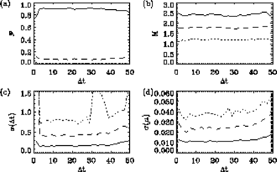
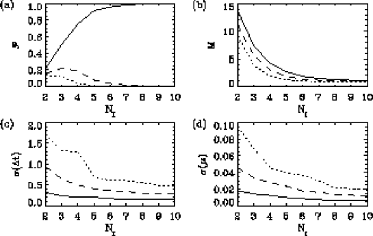
Time delay :
Figure 10 presents the results for changing the value of the time delay between and . This corresponds to the range which is considered as the range of potential time delay values and for which the function is calculated. The graphs indicate that apart from some boundary effects the results are rather insensitive to varying . They get slightly worse, i.e. the fraction is decreasing and the errors and are increasing, for large time delays , because the errors of the reconstructed lightcurves at the epoch of the interferometric observations increase with rising due to a smaller number of error-reducing iteration steps needed for the reconstruction (cf. Figs. 4 and 3). Of course, the result also gets worse for very short values of which are then becoming comparable to the timescale of variability and the observing interval .
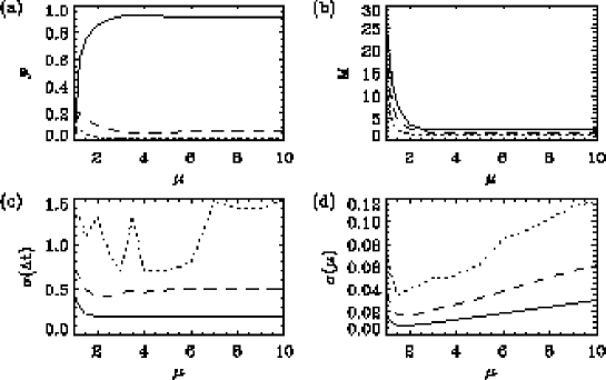
Magnification ratio :
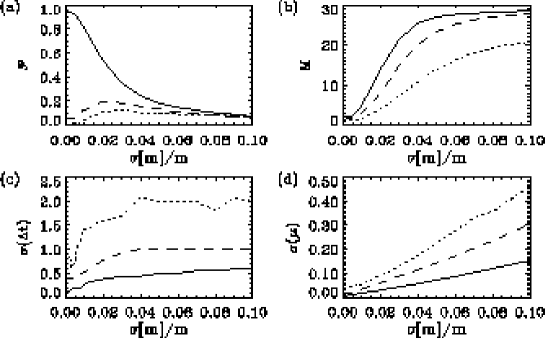
Figure 11 verifies the statement about the magnification ratio which already has been given in Sect. 3.1: The method completely fails for because then the errors due to the arbitrary initial guess do not decrease during the reconstruction process. In the diagrams the breakdown of the method for is reflected by the steep decrease of and the steep increase of the number of minima appearing in the function. For the vaules , and are remaining virtually constant. Note, however, that in this figure the relative accuracy of the flux density ratio measurements has been kept constant. For rising magnification ratio it will become increasingly difficult to measure the then also rising flux density ratios with the desired accuracy, and this will limit the applicability of the method for large .
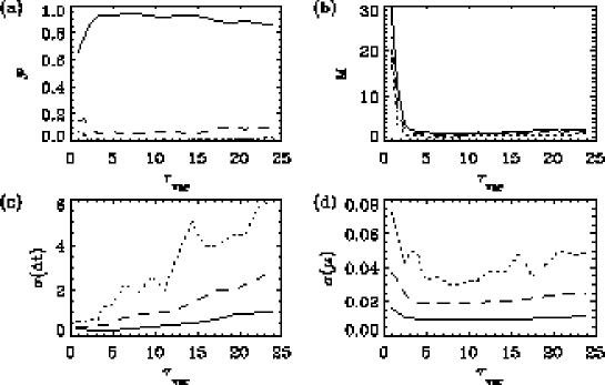
Timescale of variability :
Figure 12, showing the dependence of the results on the timescale of variability, mainly reveals two effects. For very short timescales the errors introduced by interpolating the observed lightcurve between consecutive data points become large. This leads to an increase in the number of unwanted wrong minima and to a decrease of the fraction . For slow variation, on the other hand, the number of minima roughly stays constant and is only slightly decreasing, at least in the range of timescales plotted here. However, the error in the location of the true minimum is rising then. This means that the minima in the function are becoming broader and that the accuracy of the time delay determination is reduced.
Variability :
A very important parameter is, of course, the relative variability of the source. In Fig. 13 not only has been varied, but also the noise parameter , which also includes the dispersion of the combined lightcurve, has been adapted in such a way that the absolute errors of the single-dish lightcurve measurements remain constant. Naturally for no time delay determination is possible, but for increasing variability the results improve quite quickly, and nearly reaches the ideal value of for . The simulations have not been extended to variabilities larger than because then the minima in the function are becoming very steep and narrow, which makes it more difficult to find them numerically.
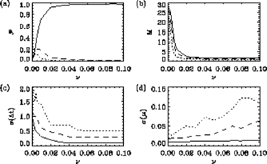
Number of interferometric observations :
Figure 14 shows the evolution of the results when increasing the number of additional interferometric observations which are used as constraints for the fit. From these diagrams it can be seen how the fraction of lightcurves for which the true minimum is the global minimum of the function rises and the number of minima and the errors in the location of the true minimum decrease. For eight flux density ratio measurements, the fraction has nearly reached and typically there is just one minimum remaining.
Interval between interferometric observations :
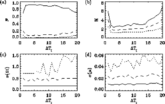
For simplicity this study has been restricted to constant time intervals between the interferometric observations. These are performed towards the end of the observing period when the reconstruction is most accurate (cf. Fig. 5). Figure 15 shows that the standard value is almost ideal for the standard parameter set. The results get worse for small which are comparable to the timescale of variability, because then consecutive flux density ratio measurements do not provide independent constraints. Therefore larger values of are adequate for more slowly varying lightcurves. Very large values for , however, are disfavourable, because then the first interferometric observations would have to be placed early on during the observing period when the errors of the reconstruction are still large.
Observing period :
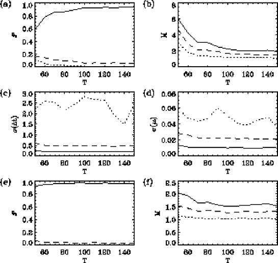
In contrast to the autocorrelation method (cf. Fig. 2a) the dependence of the results on the observing period is rather indirect for the reconstruction method. The need for a sufficiently long observing period arises from the fact that the uncertainty due to the arbitrary initial guess gradually decreases during the reconstruction process. Eventually, the errors of the reconstructed lightcurves will be dominated by the observational errors of the single-dish measurements and will therefore roughly stay constant with time. This behaviour is reflected by the diagrams a to d of Fig. 16. For small the results improve when extending the observation period, because then the interferometric measurements are still performed at epochs for which the reconstruction is affected by the initial errors. But since these have already dropped out at the respective epochs for , prolonging the observation period beyond that value does not improve the results any longer.
Figure 16e and f show the effects of reducing the interval of potential time delay values, for which the reconstruction is done and for which the function is calculated, from to . Of course, this significantly improves the results, because then the wrong minima which are located in the interval are excluded from the analysis. In addition, the worsening of the results for is not so serious in this case, because these problems preferentially arise due to the large values for which the errors of the reconstruction are decreasing slower, and just these values have been excluded here.

Observing interval :
The effects of changing the observing interval for the single-dish measurements are conveniently demonstrated by inspecting the contours for an individual lightcurve realization. We have mentioned before that for calculating the reconstruction with values which are not integer multiples of , the observed combined lightcurve has to be interpolated which in general causes additional errors for the reconstructed lightcurves. This leads to the effect that integer multiples of can be excluded as values for the time delay with a higher confidence than non-integer multiple values and that wrong minima are preferentially appearing at the latter ones. This is drastically demonstrated by the example shown in Fig. 17a. Here the observing interval has been changed to and a variety of wrong minima are showing up. Note, however, that the global minimum still corresponds to the true minimum. In practice the effect described here will be alleviated to some extent by irregular observing intervals. The example plotted in Fig. 17b shows that the adequate choice of the observing interval sensitively depends on the timescale of variability. Despite using the same observing interval of as in Fig. 17a only one minimum is appearing here and the time delay can unambiguously be determined, because in this case the variability timescale is very much longer and therefore the interpolation errors are not so serious.
Observing erros :
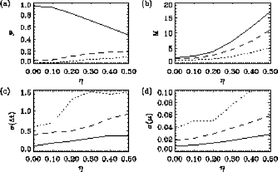
From Fig. 18 it can be seen that fairly accurate single-dish flux density measurements are required for the method to work. For the standard parameter values the rms errors should not exceed of the dispersion of the lightcurve itself (). The reason for the sensitivity to is, of course, that errors in the observed total lightcurve directly translate into errors of the reconstructed individual lightcurves and flux density ratios. In particular, it is desirable to determine the total flux density to a very good accuracy at the epochs of the interferometric observations, because the errors of these values contribute to the errors of the predicted flux density ratios to a large extent (cf. Eqs. (16) and (17)).
Flux density ratio erros :
A crucial parameter is the accuracy of the additional constraints which are provided by the interferometric observations. Figure 19 depicts the dependence of the results on the relative error of the flux density ratio measurements. For the standard parameter values this error should not exceed .
To complete the discussion of the parameter dependence we mention here that the effects of increasing the error of the average combined flux density, which enters in Eq. (17), are negligible even for high values. Furthermore, changing the shape of the power spectrum which is used for generating the simulated lightcurves does not affect the results significantly.
3.5 determination for individual realizations
Figure 20a shows the contours for one example lightcurve generated with the standard parameter values (Tables 1 and 2). In this case two minima appear with values low enough to be considered as candidates for the true minimum. Ideally one would like to include enough interferometric measurements so that only one sufficiently deep minimum is remaining. But here we have chosen this example in order to illustrate how we can determine probabilities for particular minima to be the true minimum in such cases and how error ranges for the time delay and the magnification ratio can be obtained. The former will not be possible without making use of the simulations, but concerning the latter point we can again apply statistics.

Figure 21 verifies that the distribution of the difference between the values at the exact parameter values (, ) and at the true minimum is following a -distribution with 2 degrees of freedom, as it is theoretically expected for two fit parameters ( and ). Assuming that a particular minimum is indeed the true minimum, we can use the limiting values indicated in Fig. 21 to obtain confidence regions for the time delay and the magnification ratio . This has been done in plots c and d of Fig. 20 for the minima at and , respectively. Note that for determining confidence intervals for the time delay alone, irrespective of the magnification ratio, the -distribution with 1 degree of freedom has to be used for .

In order to quantify the probability for the respective minima to be the true minimum we distinguish the following two cases:
-
A:
The minimum at is the true minimum. Then the minimum at necessarily has to be the lowest wrong minimum.
-
B:
The minimum at is the true minimum. This means that the minimum at is the lowest wrong minimum.
Here we are neglecting the possibility that both of these minima are wrong, because this would imply that the true minimum is at a value beyond the limit and thus very far in the exponentially decreasing tail of the probability density distribution (cf. Fig. 9)999Note that the limit which has been used for the contours in Fig. 20a and which is indicated by the vertical line in Fig. 9 is derived from the -distribution with degrees of freedom and therefore is conservative for the purpose of excluding wrong minima. To do that the distribution with degrees of freedom would be adequate. See the discussion at the end of Sect. 3.3.. In Fig. 22a we again show the probability density distribution for the true minimum, represented by the theoretical -distribution with 3 degrees of freedom, and the probability density distribution for the lowest wrong minimum as determined from the simulations. In the following we denote the values at the minimum with and those at the minimum with . In the figure these values are marked with vertical lines, the solid line for and the dashed line for . In case A, i.e. being the true minimum, the value for is drawn from the distribution and therefore is drawn from , whereas for case B it is vice versa. In Fig. 22b the values at the lowest wrong minimum have been plotted against the value at the true minimum for the individual realizations of the lightcurve simulations. Since this scatter plot shows no correlation between these values, we can treat and as independent distributions.
This allows us to assign probabilities to the cases A and B:
Concerning the determination of the time delay and the magnification ratio we can therefore make the following statements. With a probability of the minimum at is the true minimum. Then confidence regions for the time delay and the magnification ratio are given by Fig. 20b. The probability for being the true minimum is . In this case the confidence regions for and are given by Fig. 20c. In view of the much higher probability of case A, which is indeed the true one, this result could also be phrased as: The error level for restricting the time delay to be with confidence regions as shown in Fig. 20b is .
At this point a few cautionary remarks should be added. The probabilities derived here rely on the distribution of the wrong minima which cannot be described by statistics and therefore has to be determined from the simulations. Hence, in applications to real observations it is important to generate a set of simulated lightcurves which satisfactorily reflects the variability characteristics of the observed lightcurve. Determining the confidence regions in Fig. 20b and c, however, solely relies on statistics and does not require any simulations. Of course, for any fit it is essential to use error estimates which are really reflecting the statistical uncertainties of the measurements and not, e.g., the observer’s predilection for giving conservative limits.
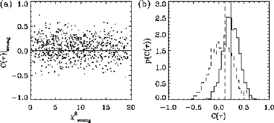
To conclude this section we demonstrate how the results can be improved by additionally taking into account the information contained in the autocorrelation function. In Fig. 23a the value of the autocorrelation function for the lag corresponding to the time delay value of the lowest wrong minimum has been plotted against the value at that minimum for the individual lightcurve realizations. The scatter plot indicates that there is no correlation between these two quantities and that on average the value is zero, i.e. there is no enhanced autocorrelation for values corresponding to the values of wrong minima. This implies that the lightcurve reconstruction method and the autocorrelation method are completely independent techniques for determining the time delay. Figure 23b depicts the distributions of the autocorrelation values for lags corresponding to the value of the true minimum (solid line) and of the lowest wrong minimum (dashed line). The latter distribution is centered around , whereas the former is shifted to higher autocorrelation values. The reason for this is, of course, that the true minimum is roughly located at the correct time delay and so the effect discussed in Sect. 2 leads to an enhanced autocorrelation. From the large overlap of these distributions and from the small separation of the vertical lines in this plot, which in analogy to Fig. 22a denote the values for the two minima of the example case, it is clear that the autocorrelation function cannot improve the results drastically. Nevertheless, including this additional information in a similar analysis as above leads to probability values of and and thus the error level for tying oneself down to as the value for the time delay could be reduced from to .
4 Discussion and conclusions
In the first part of this paper we have shown that an analysis of the autocorrelation function of the total lightcurve of gravitational lens systems can in principle be used to determine its time delay. In practice, however, a fairly long observing time is required to make sure that the measured autocorrelation function reliably reflects the lightcurve’s underlying statistical properties. In addition, the characteristic time scale for the source variability has to be considerably shorter then the time delay, and the magnification ratio should be close to unity in order for the autocorrelation function to develop distinct time delay features.
It is interesting to note that it has been proposed by Press (1996) that in certain cicumstances time autocorrelation effects on unresolved, time-varying objects could be used to establish otherwise undetectable (micro-) lens systems. In view of the results shown in Sect. 2 a detection of the time delay effect via an analysis of the autocorrelation function seems to require a delicate fine tuning between the involved time scales, i.e. the observing interval, the time scale of variability, the time delay, the observing period and possibly the “life time” of the lensing configuration. However, using different approaches might be more promising, especially for non-gaussian random processes. Consider, as an extreme example, an intrinsic source lightcurve consisting of a characteristic series of sharp peaks. In such a “burst-scenario” a time delay could be easily determined from the repetition of the features which is then showing up in the observed lightcurve of the lens system.
In Sect. 3 we introduced the “lightcurve reconstruction method”. We demonstrated that it is possible to reconstruct the individual lightcurves of a gravitational lens system from the observed total lightcurve by assuming values for the time delay and the magnification ratio. The reconstructed lightcurves are most accurate at the end of the observing period, because errors introduced by an arbitrary initial guess are gradually decreasing during the reconstruction process. However, this is not true for a magnification ratio close to unity and the method is therefore not applicable in such cases. In general it will be impossible without additional information to single out the true time delay from all possible reconstructions with potential values for the time delay and the magnification ratio. (A counterexample for which this might indeed be feasible by assuming some reasonable shape for the correctly reconstructed lightcurves is the highly non-gaussian burst-scenario outlined above.) However, interferometric measurements of the flux density ratio (at the same frequency as the total flux density monitoring!) provide an excellent means for checking the consistency of the various reconstructions and eventually determining the time delay unambiguously.
With simulations we investigated the dependence of the method on various parameters. Naturally the variability of the lightcurve turns out to be an essential parameter – as it is the case for any time delay determination technique. In addition, a fairly high accuracy for the total flux density monitoring observations as well as for the additional interferometric flux density ratio measurements is desirable. In contrast to the autocorrelation method the lightcurve reconstruction also works for rather slowly varying lightcurves, although increasing the time scale of variability leads to larger confidence intervals for the time delay. (That lightcurves with fairly slow variability still contain information about the time delay can also be seen from van Ommen et al.’s (1995) analysis of the lightcurve of PKS1830-211, a lens system with two compact images and an Einstein ring. They use simple linear fits to the slowly varying total lightcurve and combine these with interferometric flux density ratio measurements to get an estimate for the time delay. However, the confidence intervals for this value are still quite large.) Of course, the simulations that we have performed just show the general trends and cannot cover the parameter space completely. For a given lens system and observation programme some unfavourable parameter values could be compensated by another parameter being much more adequate and thus leading to equivalently good results.
In principle the method described here could be used for radio as well as for optical lightcurves. However, there are several arguments against optical wavelengths. If the time scale of variability is short, a small observing interval is essential to sample the lightcurve accurately and a larger gap due to bad weather would have drastic effects on the quality of the reconstruction. In addition, microlensing effects which cannot properly be acounted for in this method can be important in the optical. However, if the microlensing time scale is considerably larger than the time delay and the observing period, this will only result in a change of the effective magnification ratio and the method can still be applied. Finally, a very important reason to perform such observations at radio frequencies is that the most promising lens systems for determining the Hubble constant consist of double images of radio-loud sources and an associated ring of extended emission. From these Einstein rings the system B0218+357 mentioned in the introduction probably is the best candidate at the moment. The time delay for this system is expected to be roughly between 8 and 20 days which is reflecting our current knowledge (or rather ignorance) of the Hubble constant and uncertainties in the lens model. (A detailed model for this system which takes into account the information provided by the Einstein ring still has to be made.) The preliminary value of for the time delay obtained by Corbett et al. (1996) is consistent with this range. Reliable estimates for the time scale and the amplitude of the source variability are required in order to design an optimal observing strategy and to specify the number of interferometric observations needed for a definite determination of the time delay by using the lightcurve reconstruction method. However, combining a single-dish monitoring programme of two or three months with five to ten additional interferometric constraints should be adequate to determine the time delay reliably.
For the system PKS1830-211 the discovery of molecular absorption lines by Wiklind & Combes (1996) opens an interesting new possibility to determine the time delay from unresolved single-dish monitoring observations only. Apparently only one of the two source images is covered by a molecular cloud, and this allows one to determine the flux density ratio from molecular spectroscopy. Combining this with the total flux density it is possible to calculate the individual lightcurves and apply a cross-correlation analysis in order to obtain the time delay. However, the lightcurve reconstruction method could be used in this case as well, with the advantage of a much cleaner error treatment, because it uses the direct observables total flux density and flux density ratio.
Acknowledgements: We thank Hans-Walter Rix for stimulating discussions. This work was supported by the “Sonderforschungsbereich 375-95 für Astro-Teilchenphysik” der Deutschen Forschungsgemeinschaft.
References
- [1] Bernstein G.M., Tyson J.A., Kochanek C.S., 1993, AJ 105, 816
- [2] Corbett E.A., Browne I.W.A., Wilkinson P.N., Patnaik A.R., 1996, in Kochanek & Hewitt (1996)
- [3] Grogin N.A., Narayan R., 1996, ApJ submitted, astro-ph/9512156
- [4] Kochanek C.S., 1991, ApJ 382, 58
- [5] Kochanek C.S., Hewitt J.N. (eds.), 1996, Astrophysical applications of gravitational lensing. Kluwer, Dordrecht (in press)
- [6] Patnaik A.R., Browne I.W.A., King L.J., et al., 1993, MNRAS 261, 435
- [7] Patnaik A.R., Porcas R.W., Browne I.W.A., 1995, MNRAS 274, L5
- [8] Press W.H., Rybicki G.B., Hewitt J.N., 1992a, ApJ 385, 404
- [9] Press W.H., Teukolsky S.A., Vetterling W.T., Flannery B.P., 1992b, Numerical Recipes in FORTRAN. Cambridge University Press, Cambridge
- [10] Press W.H., 1996, in Kochanek & Hewitt (1996)
- [11] Refsdal S., 1964, MNRAS 128, 307
- [12] van Ommen T.D., Jones D.L., Preston R.A., Jauncey D.L., 1995, ApJ 444, 561
- [13] Walsh D., Carswell R.F., Weymann R.J., 1979, Nat 279, 381
- [14] Wiklind T., Combes F., 1996, Nat 379, 139
- [15]