Reanalysis of the association of high-redshift 1-Jansky quasars with IRAS galaxies

Abstract

We develop a new statistical method to reanalyse angular correlations between background QSOs and foreground galaxies that are supposed to be a consequence of dark matter inhomogeneities acting as weak gravitational lenses. The method is based on a weighted average over the galaxy positions and is optimized to distinguish between a random distribution of galaxies around QSOs and a distribution which follows an assumed QSO-galaxy two-point correlation function, by choosing an appropriate weight function. With simulations we demonstrate that this weighted average is slightly more significant than Spearman’s rank-order test which was used in previous investigations. In particular, the advantages of the weighted average show up if the two-point correlation function is weak.

We then reanalyze the correlation between high-redshift 1-Jansky QSOs and IRAS galaxies, taken from the IRAS Faint Source Catalog; these samples were analyzed previously using Spearman’s rank-order test. In agreement with the previous work, we find moderate to strong correlations between these two samples; considering the angular two-point correlation function of these samples, we find a typical scale of order $5^{\prime}$ from which most of the correlation signal derives. However, the statistical significance of the correlation changes with the redshift slices of the QSO sample one considers. Comparing with simple theoretical estimates of the expected correlation, we find that the signal we derive is considerably stronger than expected. On the other hand, recent direct verifications of the overdensity of matter in the line-of-sight to high-redshift radio QSOs obtained from the shear field around these sources, indicates that the observed association can be attributed to a gravitational lens effect.

1 Introduction

It was argued by Bartelmann & Schneider ([1991], [1992], [1993a], [1993b]) that a statistical association between foreground galaxies and distant, radio-loud background sources, as claimed to be observed by Fugmann ([1988], [1990]), can be caused by gravitational lensing effects due to large-scale structures of the dark-matter distribution in the Universe. Using Spearman’s rank-order test to investigate the association of 1Jy sources with Lick galaxies and IRAS galaxies, they indeed found correlations at a high level of significance (Bartelmann & Schneider [1993b], [1994], hereafter BS). A quantification of such correlations could prove to be a unique tool for directly probing dark-matter inhomogeneities. It is therefore very important to verify the results of these analyses with independent methods and, if possible, to improve their statistical significance, or to obtain more detailed information about the association, e.g. the amplitude of the correlation function or a characteristic angular scale. Other groups have shown a statistically significant association between other samples of QSOs and foreground matter: Rodrigues-Williams & Hogan ([1994]), Seitz & Schneider ([1995]) and Wu & Han ([1995]) have shown evidence for an overdensity of Abell and Zwicky clusters around high-redshift QSOs, and Hutchings ([1995]) has studied the distribution of galaxies around seven QSOs at $z=2.3$, and found a statistically significant excess around all of them. Whereas he did not interpret this result as being due to gravitational lensing, it appears to be a more natural explanation than assuming that these galaxies are spatially associated with the QSOs, which would imply an enormous luminosity evolution.

Direct evidence for the presence of lensing matter in the line-of-sight towards high-redshift QSOs was obtained by Fort et al. ([1995]) who imaged faint galaxies around several high-redshift 1Jy QSOs. For several of them, they obtained clear evidence for a coherent shear pattern around these QSOs, which can be attributed to local concentrations of faint galaxies. These concentrations may indicate the presence of a group or a cluster, but they are so faint optically that they would not appear in any cluster catalog. What this might suggest is that there exists a population of clusters with a much larger mass-to-light ratio than those clusters which are selected because of their high optical luminosity, i.e., which appear in optically-selected cluster catalogs. If these findings are confirmed (e.g., by HST observations), one has found a way to obtain a mass-selected sample of clusters and/or groups.

In the following sections, we introduce a new approach to test for correlations (Sect. 2), and use numerical simulations (Sect. 3) to demonstrate that it is applicable and can lead to an improvement of the significance of the results, if compared to Spearman’s rank-order test. Section 4 then presents the results that are obtained with our method for 1Jy quasars and IRAS galaxies. In addition, we perform further simulations to compare our findings with what is expected from theory. Finally we summarize and present our conclusions in Sect. 5.

2 Method

In this section we define our new correlation test, based on a weighted average. Furthermore we show how it can be applied for measuring quasar-galaxy associations and how to make use of an a priori guess (e.g. from theory) of the quasar-galaxy correlation function to find an optimum weight function.

For readers who lack the patience to follow the arguments below, we now give a brief summary of the results of this section, which should enable him or her to directly go to Sect. 2.3.

Given a sample of QSOs, and a sample of galaxies around these QSOs, such that $\phi_{i}$ is the angular separation of the $i$-th galaxy from its associated QSO we then define a correlation coefficient $r_{g}$ by

$$r_{g}=\frac{1}{N}\sum_{i=1}^{N}g(\phi_{i})\ ,$$

where $g(\phi)$ is a weight function. Given an assumed two-point correlation function $\xi_{\rm qg}(\phi)$ between QSOs and galaxies, we show that the optimal choice of the weight function to allow the distinction between the assumed two-point correlation function and a random distribution of galaxies relative to the QSOs is given by

$$g(\phi)=a\,\xi_{\rm qg}(\phi)+b\quad,$$ (1)

with arbitrary ($a\neq 0$) constants $a$, $b$.

2.1 Definitions

For any realisation $\left(\vec{x},\vec{y}\right)$ of a pair $\left(\vec{X},\vec{Y}\right)$ of $n$-dimensional random variables $\vec{X}:=\left(X_{1},\ldots,X_{n}\right)$ and $\vec{Y}:=\left(Y_{1},\ldots,Y_{n}\right)$ we define a correlation coefficient by

$$r\left(\vec{x},\vec{y}\right):=\sum_{i=1}^{n}g\left(x_{i}\right)\cdot f\left(y_{i}\right)$$ (2)

with arbitrary functions $g$ and $f$. Formally, this can be understood as an average of $g\left(x_{i}\right)$ weighted with $f\left(y_{i}\right)$ (or vice versa), but without the usual normalisation of the weights. In our application below, the vector $\vec{Y}$ denotes the counts of galaxies in $n$ concentric rings around quasars, and the vector $\vec{X}$ denotes the radii of these rings.

Given the probability density $p_{\rm o}\left(\vec{x},\vec{y}\right)$ of $\left(\vec{X},\vec{Y}\right)$ and one single realisation $(\vec{x}^{\prime},\vec{y}^{\prime})$ of two random variables, it is our aim to decide whether the assumption of $(\vec{x}^{\prime},\vec{y}^{\prime})$ being a realisation of $\left(\vec{X},\vec{Y}\right)$ can be rejected or not. For this purpose we use $p_{\rm o}\left(\vec{x},\vec{y}\right)$ to determine the distribution of the correlation coefficient for realisations of $\left(\vec{X},\vec{Y}\right)$, i.e. we calculate the cumulative probability

$$P_{\rm o}\left(r\geq R\right)=\int\!\!\cdots\!\!\int{\rm d}^{n}x\,{\rm d}^{n}y\,p_{\rm o}\left(\vec{x},\vec{y}\right)\,\Theta\left(r\left(\vec{x},\vec{y}\right)-R\right)$$

for $r$ taking a value greater than or equal to some threshold $R$ for any realisation of $\left(\vec{X},\vec{Y}\right)$.

Now suppose we find a value $R^{\prime}:=r(\vec{x}^{\prime},\vec{y}^{\prime})$ of the correlation coefficient of $(\vec{x}^{\prime},\vec{y}^{\prime})$, and let us define $\varepsilon$ as

$$\varepsilon:=P_{\rm o}\left(r\geq R^{\prime}\right)\ \ .$$

Premising $(\vec{x}^{\prime},\vec{y}^{\prime})$ to be a realisation of $\left(\vec{X},\vec{Y}\right)$, we know that $\varepsilon$ is the probability of the correlation coefficient to give a result greater than or equal to $R^{\prime}$. Hence, if $\varepsilon$ happens to be very small (or very large because then $1-\varepsilon=P_{\rm o}(r<R^{\prime})$ is very small) we might reject our premise but rather assume $(\vec{x}^{\prime},\vec{y}^{\prime})$ to be drawn from a different pair of random variables $(\vec{X}^{\prime},\vec{Y}^{\prime})$.

As a consequence of this strategy, we would erroneously conclude for a fraction $\varepsilon$ of all realisations of $\left(\vec{X},\vec{Y}\right)$ that they are not drawn from $\left(\vec{X},\vec{Y}\right)$, because their correlation coefficient is greater than or equal to $R^{\prime}$. Throughout this paper the value of $\varepsilon$ will therefore be called the ‘error level’.

Up to now, we did not specify the functions $g$ and $f$. By intuition one is lead to the idea that they should be adapted to the given problem. Imagine we want to check whether $(\vec{x}^{\prime},\vec{y}^{\prime})$ can be considered a realisation of $\left(\vec{X},\vec{Y}\right)$. Furthermore, we suspect that $(\vec{x}^{\prime},\vec{y}^{\prime})$ has been drawn from different random variables $(\vec{X}^{\prime},\vec{Y}^{\prime})$ with a corresponding probability density $p_{\rm a}(\vec{X}^{\prime},\vec{Y}^{\prime})$, where the subscript ‘a’ stands for the ‘alternative hypothesis’. What we want to achieve then is that the correlation test allows for an optimum distinction between these two hypotheses. For both of them we can, in principle, derive the probability density of the correlation coefficient $r$ from the equations

$$p_{\rm o}\left(r\right) = \int\!\cdots\!\int{\rm d}^{n}x\,{\rm d}^{n}y\,p_{\rm o}\left(\vec{x},\vec{y}\right)\,\delta\left(r\left(\vec{x},\vec{y}\right)-r\right)\ \ ,$$

$$p_{\rm a}\left(r\right) = \int\!\cdots\!\int{\rm d}^{n}x\,{\rm d}^{n}y\,p_{\rm a}\left(\vec{x},\vec{y}\right)\,\delta\left(r\left(\vec{x},\vec{y}\right)-r\right)\ \ ,$$

where $\delta\left(r\right)$ denotes Dirac’s delta function. The first definition one can think of to quantify the distinction between $p_{\rm o}\left(r\right)$ and $p_{\rm a}\left(r\right)$ is the mean error level

$$\left\langle P_{\rm o}\left(r\geq R\right)\right\rangle:=\int P_{\rm o}\left(r\geq R\right)\,p_{\rm a}\left(R\right)\,{\rm d}R\ \ .$$ (3)

According to the preceding explanations the mean error level should be as small (or large) as possible.

If $p_{\rm o}\left(r\right)$ and $p_{\rm a}\left(r\right)$ are characterised by a single (e.g. Gaussian-like) peak, we can also expect the quantities

$$Q_{1} := \frac{\left\langle r\right\rangle_{\rm a}-\left\langle r\right\rangle_{\rm o}}{\sigma_{\rm o}}\ \ ,$$ (4)

$$Q_{2} := \frac{\left\langle r\right\rangle_{\rm a}-\left\langle r\right\rangle_{\rm o}}{\sigma_{\rm a}}\ \ ,$$ (5)

together with the definitions

$$\left\langle r\right\rangle_{\rm a,o} := \int r\,p_{\rm a,o}\left(r\right)\,{\rm d}r\ \ ,$$

$$\sigma_{\rm a,o} := \left[\int\left(r-\left\langle r\right\rangle_{\rm a,\rm o}\right)^{2}p_{\rm a,o}\left(r\right){\rm d}r\right]^{1/2}\ \ ,$$

to be good measures of the distinction between $p_{\rm o}\left(r\right)$ and $p_{\rm a}\left(r\right)$. Figure 1 illustrates this concept. In the following section we want to specify the functions $g$ and $f$. We claim that by maximizing either $\left|Q_{1}\right|$ or $\left|Q_{2}\right|$ we can find $g$ and $f$ such that $r$ as a test for quasar-galaxy correlations operates close to its optimum sensitivity, which we will demonstrate in Sect. 3 by means of numerical simulations.

Figure 1: A simple measure of the distinction of two Gaussian-like distributions is the separation of their mean values in units of either one of their standard deviations. The shaded area represents the error level $P_{\rm o}\left(r\geq\left\langle r\right\rangle_{\rm a}\right)$.

2.2 Quasar-galaxy correlations

We now want to apply these theoretical concepts to the associations between quasars and galaxies by analysing the radial distribution of galaxies in the vicinity of quasars from a given sample. Suppose that for each quasar we have a list of relative angular coordinates of galaxies within a certain (preferably circular) field around the quasar.

One way to investigate the galaxy distribution is to merge these lists into one total list corresponding to a total galaxy field. For the correlation test we choose an inner and an outer angular radius, $\phi_{\rm in}$ and $\phi_{\rm out}$, to define a ring $\left[\phi_{\rm in},\phi_{\rm out}\right]$ within the total field which is divided into $n$ concentric annuli $\left[\varrho_{i},\varrho_{i+1}\right]$ by the $n+1$ radii

$$\varrho_{i}:=\phi_{\rm in}+\left(i-1\right)\cdot\frac{\phi_{\rm out}-\phi_{\rm in}}{n}\ \ ,\ \ \ i=1,\ldots,n+1\ .$$ (6)

Let $z_{i}$ denote the number of galaxies within $\left[\varrho_{i},\varrho_{i+1}\right]$ and set $\vec{x}:=\left(\varrho_{1},\ldots,\varrho_{n}\right)$, $\vec{y}:=\left(z_{1},\ldots,z_{n}\right)$. Then, the correlation coefficient (2) reads

$$r=\sum_{i=1}^{n}g\left(\varrho_{i}\right)\,f\left(z_{i}\right)\ \ .$$ (7)

If we increase the number $n$ of sub-rings, while the total number $N:=z_{1}+\cdots+z_{n}$ of galaxies within $\left[\phi_{\rm in},\phi_{\rm out}\right]$ is constant, we will eventually reach the situation where each of the sub-rings contains one galaxy at most, i.e. $z_{i}=0$ or $1$ for $i=1,\ldots,n$. At that point $f\left(z_{i}\right)$ in Eq. (7) will only take the two values $f\left(0\right)$ and $f\left(1\right)$, so obviously $f\left(0\right)\neq f\left(1\right)$ is required, because otherwise $r$ would become independent of the galaxy distribution and useless for the correlation analysis. From these statements it follows that we can find two constants $a$ and $b$ such that, for $z_{i}=0$ or $1$,

$$\widetilde{f}\left(z_{i}\right):=a\cdot f\left(z_{i}\right)+b=\frac{z_{i}}{N}\ \ ,\ \ \ i=1,\ldots,n\ ,$$

which in turn results in a linear transformation of the correlation coefficient

$$\widetilde{r}:=\sum_{i=1}^{n}g\left(\varrho_{i}\right)\,\widetilde{f}\left(z_{i}\right)=a\cdot r+b^{\prime}\ \ ,$$

where

$$b^{\prime}=b\cdot\sum_{i=1}^{n}g\left(\varrho_{i}\right)\ .$$

A substitution of $r$ with $\widetilde{r}$ in Eqs. (4) and (5) yields $\widetilde{Q}_{1,2}={\rm sign}\left(a\right)\cdot Q_{1,2}$ and $|\widetilde{Q}_{1,2}|=\left|Q_{1,2}\right|$. This shows that the linear transformation $f\rightarrow\widetilde{f}$ does not influence the maximisation of $\left|Q_{1}\right|$ or $\left|Q_{2}\right|$, our means for optimizing the correlation test. If $n$ is large enough (i.e. $z_{i}=0,1$) we can therefore choose $f\left(z_{i}\right)=z_{i}/N$ without loss of generality, so we get

$$r:=\frac{1}{N}\sum_{i=1}^{n}z_{i}\,g\left(\varrho_{i}\right)\ \ .$$

Furthermore, if the radial positions of the $N$ galaxies within $\left[\phi_{\rm in},\phi_{\rm out}\right]$ are denoted with $\phi_{j}$, $j=1,\ldots,N$, it is clear that with increasing $n$ the radii of sub-rings $\left[\varrho_{i},\varrho_{i+1}\right]$ containing one of the galaxies approach the values $\phi_{j}$. As $z_{i}=0$ for all the other sub-rings, we can define

$$r_{g}\left(\phi_{1},\ldots,\phi_{N}\right):=\lim_{n\to\infty}\frac{1}{N}\sum_{i=1}^{n}z_{i}\,g\left(\varrho_{i}\right)=\frac{1}{N}\sum_{j=1}^{N}g\left(\phi_{j}\right)\ \ .$$ (8)

Note that, by taking the limit $n\to\infty$, we finally got rid of the arbitrary number $n$ of sub-rings within the galaxy field under consideration. This is a first advantage of the ‘weighted average’ correlation test compared to Spearman’s rank test, which was applied in earlier investigations (e.g. BS) and required a binning of the data.

In the following, we will assume the galaxies to be distributed independently of one another. That means the galaxy distribution within $\left[\phi_{\rm in},\phi_{\rm out}\right]$ can be described by a one-dimensional radial probability density $p\left(\phi\right)$, which defines the probability $p\left(\phi\right){\rm d}\phi$ for a single galaxy to be found at some position between two given angular radii $\phi$ and $\phi+{\rm d}\phi$. Because of galaxy-galaxy correlations our assumption is a simplification and does not hold in general. In Sect. 4 we argue that it should nevertheless be applicable in this analysis.

One approach to statistically prove an association between quasars and galaxies is to start with the ‘null-hypothesis’ of no association and then try to reject it with the help of the correlation coefficient (2). Normally the null-hypothesis will be characterised by a radial probability density $p_{\rm o}\left(\phi\right)\sim\phi$, corresponding to a Poissonian galaxy distribution. However, if the galaxy fields around the individual quasars that we merge to form the total galaxy field do not all have the same angular radius or are irregularly shaped, $p_{\rm o}\left(\phi\right)$ may look quite differently. Therefore, we will write

$$p_{\rm o}\left(\phi\right)=:c_{\rm o}\cdot G\left(\phi\right)\ \ ,$$

using a geometrical factor $G\left(\phi\right)\geq 0$ and a normalisation constant $c_{\rm o}>0$ to meet the condition

$$\int_{\phi_{\rm in}}^{\phi_{\rm out}}p_{\rm o}\left(\phi\right){\rm d}\phi=c_{\rm o}\cdot\int_{\phi_{\rm in}}^{\phi_{\rm out}}G\left(\phi\right){\rm d}\phi=1\ \ .$$

The theory of gravitational lenses, together with some cosmological model, can give quantitative predictions about the expected angular quasar-galaxy two-point correlation function $\xi_{\rm qg}\left(\phi\right)$ (cf. Bartelmann [1995]). For galaxy positions which are independent of one another, this implies a one-dimensional probability density $p_{\rm a}\left(\phi\right)$, which we will write in the form

$$p_{\rm a}\left(\phi\right)=:c_{\rm a}\left(\phi\right)\cdot G\left(\phi\right)\ \ ,$$

where $c_{\rm a}\left(\phi\right)$ is related to $\xi_{\rm qg}\left(\phi\right)$ via the expression

$$c_{\rm a}\left(\phi\right)=C\cdot\left[1+\xi_{\rm qg}\left(\phi\right)\right]\ \ .$$

As before, normalisation is required, i.e.

$$\int_{\phi_{\rm in}}^{\phi_{\rm out}}p_{\rm a}\left(\phi\right){\rm d}\phi=C\cdot\int_{\phi_{\rm in}}^{\phi_{\rm out}}\left[1+\xi_{\rm qg}\left(\phi\right)\right]G\left(\phi\right){\rm d}\phi=1\ \ .$$

Given an estimate of $\xi_{\rm qg}\left(\phi\right)$ from theory we suspect that the true distribution of galaxies might be described by $p_{\rm a}\left(\phi\right)$, so we want the correlation coefficient (8) to be optimised for a distinction between $p_{\rm o}\left(\phi\right)$, representing the null-hypothesis, and $p_{\rm a}\left(\phi\right)$. Applying definition (4) this can be achieved by choosing the weight function $g\left(\phi\right)$ such that the global maximum of $\left|Q_{1}\right|$ is reached. A variational calculation, shown in Appendix A.1, yields Eq. (1),

$$g\left(\phi\right)=a\,\xi_{\rm qg}\left(\phi\right)+b\ \ ,$$ (9)

with arbitrary ($a\neq 0$) constants $a$ and $b$. Similarly, one finds

$$g\left(\phi\right)=\frac{a^{\prime}}{1+\xi_{\rm qg}\left(\phi\right)}+b^{\prime}$$ (10)

when maximising $\left|Q_{2}\right|$. Such an optimisation of the correlation test is most important if $p_{\rm o}\left(\phi\right)\approx p_{\rm a}\left(\phi\right)$, i.e. $\xi_{\rm qg}\left(\phi\right)\ll 1$, because in this case it will be most difficult to rule out one of the possibilities. In the interesting regime of $\xi_{\rm qg}\ll 1$, however, the expansion $\left(1+\xi\right)^{-1}\approx 1-\xi$ implies Eqs. (9) and (10) to be nearly equivalent. Moreover, Appendix A.2 gives the proof that the weight function (9) is also a stationary point of the mean error level $\left\langle P_{\rm o}\left(r_{g}\geq R\right)\right\rangle$, as long as $\xi_{\rm qg}\left(\phi\right)\ll 1$.

2.3 Numerically derived quasar-galaxy two-point correlation function

The theoretically expected angular two-point correlation function between background quasars and foreground galaxies has been derived by Bartelmann ([1995]) for cold dark matter (CDM) and hot dark matter (HDM) Einstein-de Sitter cosmological models with linearly evolved perturbation spectra. For the following analyses we will pick out the quasar-galaxy correlation function $\xi_{\rm qg}\left(\phi\right)$ which Bartelmann extracted from a numerical simulation of a CDM universe with $H_{\rm o}=100\,{\rm km/(s\,Mpc)}$ taking into account galaxies up to $21^{\rm st}$ magnitude. Figure 2 shows plots of $\xi_{\rm qg}\left(\phi\right)$ from the numerical simulation (solid line) and of the approximation

$$\xi_{\rm qg}\left(\phi\right)\approx\xi^{\prime}\left(\phi\right):=\alpha\,\left(\phi_{\rm o}+\phi/{\rm deg}\right)^{-2.4}\ \ ,$$ (11)

with $\alpha=0.0036$ and $\phi_{\rm o}=0.24$ (dashed line). Whereas Bartelmann’s correlation functions are all normalised such that

$$\int_{0}^{\infty}\xi_{\rm qg}\left(\phi\right)\phi\,{\rm d}\phi=0\ \ ,$$

this is obviously not true for $\xi^{\prime}\left(\phi\right)$, because $\xi^{\prime}\left(\phi\right)>0$ on $\phi\in\left[0,\infty\right]$. In this sense $\xi^{\prime}\left(\phi\right)$ is not a valid fit to $\xi_{\rm qg}\left(\phi\right)$. Nonetheless the approximation does resemble three important features of the correlation function: $\xi^{\prime}\left(\phi\right)$ is steep for small $\phi$, flattens at $\phi\approx\phi_{\rm o}$ and is very shallow for large values of $\phi$. We will therefore use $\xi^{\prime}\left(\phi\right)$ to derive an approximation to the optimum weight function. To allow for different values $H_{\rm o}=h\cdot 100\,{\rm km/(s\,Mpc)}$ of the Hubble constant we have to multiply $\phi$ by the dimensionless parameter $h$. Setting $a=1/\alpha$ and $b=0$ we thus obtain from Eq. (1)

$$g\left(\phi\right)=\left(0.24+h\,\phi/{\rm deg}\right)^{-2.4}\ \ .$$ (12)

Figure 2: Solid line: Quasar-galaxy two-point correlation function from a CDM Einstein-de Sitter cosmological model with Hubble constant $H_{\rm o}=100\,{\rm km/(s\,Mpc)}$. Dashed line: Approximation according to (11).

3 Numerical simulations

Before applying the newly introduced weighted-average correlation test to observational data we want to show the results of some numerical simulations. They have been performed in order to check whether our method is more sensitive than the Spearman’s rank-order test, and to investigate the influence of variations of the weight function.

3.1 Overview

In principle, we proceed as follows: First, a large number (we use $10^{7}$) of circular galaxy fields is generated, each of them consisting of $N$ independently and randomly chosen galaxy positions. We interpret them as a statistical sample of total galaxy fields in the case of the null-hypothesis of no quasar-galaxy correlation and use them to derive the distribution $P_{\rm o}\left(r_{g}\geq R\right)$. A second set (size: $10^{6}$) of random fields is synthesized to model observed galaxy fields with an assumed association of quasars and galaxies. Again, the coordinates are drawn independently, but this time according to some radial probability density profile $p_{\rm a}\left(\phi\right)$, which is meant to describe the correlation. For a given weight function $g\left(\phi\right)$ we calculate $\left\langle r\right\rangle_{\rm a}$ as well as $\left\langle P_{\rm o}\left(r_{g}\geq r\right)\right\rangle_{\rm a}$ from the individual values $r$ of the correlation coefficient $r_{g}$. We use these quantities to analyse the sensitivity of our weighted-average correlation test as described below.

Both the error level $P_{\rm o}\left(r_{g}\geq\left\langle r\right\rangle\right)$ of the mean correlation coefficient and the mean error level $\left\langle P_{\rm o}\left(r_{g}\geq r\right)\right\rangle$ quantify the distinction between our two simulated samples: very low values (or values near unity) signify a good distinction, values around $0.5$ a bad distinction. The effect of deviations of the weight function from its optimum $g\left(\phi\right)$ can be examined by defining a parameterized weight function $g\left(\phi,\varepsilon\right)$ such that $g\left(\phi,\varepsilon=\varepsilon_{\rm o}\right)\equiv g\left(\phi\right)$ for some $\varepsilon=\varepsilon_{\rm o}$ and repeating the simulation for a whole set of values for $\varepsilon$.

Additionally we subject each of the galaxy fields of the second sample to Spearman’s rank-order test to obtain the corresponding error level of the mean correlation coefficient and the mean error level. That allows for a direct comparison between the weighted-average method and Spearman’s rank-order test, a short description of which is given below:

• The circular galaxy field is divided into $n=25$ rings of equal area. The number $25$ has been adopted from the Bartelmann & Schneider ([1994]) analysis of quasar-galaxy associations.

• The number of galaxies within each ring is determined and ranked, yielding a scheme of ranks $\left({\cal R}_{1}^{\rm a},\ldots,{\cal R}_{25}^{\rm a}\right)$ with ${\cal R}_{i}^{\rm a}\in\left\{1,\ldots,25\right\}$.

• The distance of the rings from the center is ranked in descending order, i.e. rings closer to the center are ranked higher. The result is a second rank scheme $\left({\cal R}_{1}^{\rm b},\ldots,{\cal R}_{25}^{\rm b}\right)=\left(25,24,\ldots,1\right)$.

• Spearman’s rank-order correlation coefficient $r_{\rm s}$ is calculated from its definition as the linear correlation coefficient of the rank schemes,

  $$r_{\rm s}:=\frac{\sum_{i=1}^{n}\left({\cal R}_{i}^{\rm a}-\overline{\cal R}^{\rm a}\right)\left({\cal R}_{i}^{\rm b}-\overline{\cal R}^{\rm b}\right)}{\sqrt{\sum_{i=1}^{n}\left({\cal R}_{i}^{\rm a}-\overline{\cal R}^{\rm a}\right)^{2}}\sqrt{\sum_{i=1}^{n}\left({\cal R}_{i}^{\rm b}-\overline{\cal R}^{\rm b}\right)^{2}}}\ \ ,$$

  where

  $$\overline{\cal R}^{\rm a,b}:=\left(1/n\right)\sum_{i=1}^{n}{\cal R}_{i}^{\rm a,b}\ \ .$$

  Taking into account that the rank schemes are always permutations of $\left\{1,\ldots,n\right\}$ this expression can be simplified to

  $$r_{\rm s}=1-\frac{6\cdot\sum_{i=1}^{n}\left({\cal R}_{i}^{\rm a}-{\cal R}^{\rm b}\right)^{2}}{n\left(n^{2}-1\right)}\ \ .$$

• If the number of galaxies within each ring is independent of the distance of the ring from the center and independent of the numbers of galaxies within the other rings, then the rank schemes $\left\{{\cal R}_{i}^{\rm a}\right\}$ and $\left\{{\cal R}_{i}^{\rm b}\right\}$ are random permutations of each other. In this case the distribution of

  $$t:=r_{\rm s}\left[\left(n-2\right)/\left(1-r_{\rm s}^{2}\right)\right]^{1/2}$$

  for $n>10$ is excellently approximated by a Student-t-distribution. Therefore, the error level of Spearman’s rank-order test is given by

  $$P\left(r_{\rm s}\geq R\right)=\left\{\ \begin{array}[]{ll}\frac{1}{2}I_{1-R^{2}}\left(\frac{n-2}{2},\frac{1}{2}\right)&\mbox{for $R\geq 0$}\ \ ,\\ 1-\frac{1}{2}I_{1-R^{2}}\left(\frac{n-2}{2},\frac{1}{2}\right)&\mbox{for $R<0$}\ \ ,\end{array}\right.$$

  with $I_{z}\left(a,b\right)$ denoting the incomplete beta function

  $$I_{z}\left(a,b\right):=\frac{\int_{0}^{z}s^{a-1}\left(1-s\right)^{b-1}\,{\rm d}s}{\int_{0}^{1}s^{a-1}\left(1-s\right)^{b-1}\,{\rm d}s}\ \ .$$

3.2 Results

Figure 3: Left panel: “Correlation profile” $c_{\rm a}\left(\phi\right)$ according to expression (13). Right panel: Parameterized weight function $g\left(\phi,\varepsilon\right)$ as defined in (14) for $\varepsilon=0.75$ (solid line), $\varepsilon=0$ (dotted line) and $\varepsilon=1$ (dashed line).

In the following, all angles will be measured in degrees and treated as dimensionless quantities. On circular galaxy fields the null-hypothesis corresponds to a probability density of galaxy positions

$$p_{\rm o}\left(\phi\right)=c_{\rm o}\,G\left(\phi\right)\sim\phi\ \ .$$

Let us fix the radius of the simulated galaxy fields to $0.5$ (degrees) and set

$$G\left(\phi\right):=\phi\ \ ,$$

which requires $c_{\rm o}=8$ in order to assure the normalisation of $p_{\rm o}\left(\phi\right)$. For our first series of simulations we arbitrarily choose

$$p_{\rm a}\left(\phi\right)=c_{\rm a}\left(\phi\right)\,G\left(\phi\right):=\left(\frac{64}{3}\phi^{2}-32\phi+16\right)\cdot G\left(\phi\right)$$ (13)

to describe a hypothetical quasar-galaxy correlation on the galaxy fields (Fig. 3, left panel). Moreover we define a parameterized weight function (Fig. 3, right panel)

$$g\left(\phi,\varepsilon\right):=\left(16\varepsilon-8\right)\phi^{2}-8\varepsilon\phi+1\ \ ,$$ (14)

that satisfies the condition (1) for an optimum weight function if $\varepsilon=0.75$. From these expressions we can derive the mean correlation coefficient

$$\left\langle r\right\rangle:=\int\!\!\cdots\!\!\int\left[\frac{1}{N}\sum_{i=1}^{N}g\left(\phi_{i},\varepsilon\right)\right]\prod_{j=1}^{N}\left[p_{\rm a}\left(\phi_{j}\right)\,{\rm d}\phi_{j}\right]=\int_{0}^{0.5}g\left(\phi,\varepsilon\right)\,p_{\rm a}\left(\phi\right)\,{\rm d}\phi=\frac{7-32\varepsilon}{45}\ \ .$$ (15)

The outcome of simulations for different values of $N$ carried out as explained in the preceding section is summarized in Fig. 4. The individual plots visualize the error level of the mean correlation coefficient or the mean error level, respectively, as a function of the weight-function parameter $\varepsilon$. In the heading of each panel one can find, apart from the number of galaxies $N$, the results obtained from Spearman’s rank-order test (which are, of course, independent of $\varepsilon$), denoted by $E_{\rm S}$. Two important facts can be seen in Fig. 4:

• Both the error level of the mean correlation coefficient and the mean error level do indeed attain a minimum for a weight function near the expected optimum $g\left(\phi,\varepsilon=0.75\right)$. However, the exact position of the minimum is slightly displaced with respect to the predicted one.

• Regarding the error level of the mean correlation coefficient as well as regarding the mean correlation coefficient, the weighted-average correlation test yields a more significant distinction between the two samples of galaxy fields than Spearman’s rank-order test. This remains true even if the weight function deviates significantly from its optimum.

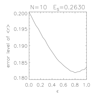
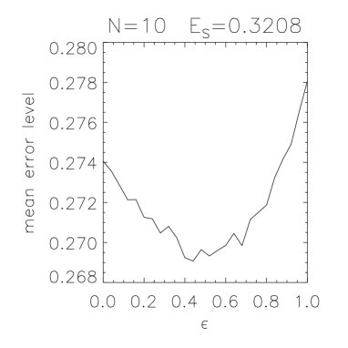
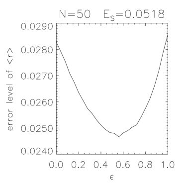
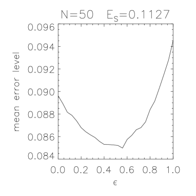
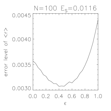
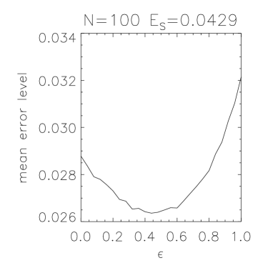
Figure 4: Error level of the mean correlation coefficient (left column) and mean error level (right column) for the weighted-average correlation test as a function of the parameter $\varepsilon$ of the weight function (14). The heading of each panel displays the corresponding results from Spearman’s rank-order test ($E_{\rm S}$) and the number of galaxies $N$.

As to the stated displacement of the minimum of the mean error level we refer to Appendix A.2 where the optimum weight function (1) is shown to approach a stationary point of the mean error level if $p_{\rm a}\left(\phi\right)$ comes close enough to $p_{\rm o}\left(\phi\right)$. This suggests that the real position of the minimum should be closer to the predicted one if the difference between $p_{\rm a}\left(\phi\right)$ and $p_{\rm o}\left(\phi\right)$ is smaller. In order to verify this, we performed a second series of simulations (in this case the null-hypothesis was modelled using only $5\cdot 10^{6}$ random fields), now setting (cf. Fig. 5, left panel)

$$p_{\rm a}\left(\phi\right)=c_{\rm a}\left(\phi\right)\,G\left(\phi\right):=\frac{32}{13}\left(2\phi^{2}-3\phi+4\right)\cdot G\left(\phi\right)\ \ .$$ (16)

The right panel of Fig. 5 displays the mean error level for $N=200$ galaxies in the total galaxy field. Clearly, the minimum is located closer to the expected position than before. We can also see from Fig. 5 that Spearman’s rank-order test is actually not too bad compared to our new test. It should also be noted that the gain in sensitivity of our new test is obtained by providing more a priori information to the test, namely the shape of the expected two-point correlation function. On the other hand, the correlation function chosen here is particularly favourable for Spearman’s rank- order test, since it can be approximated nearly as a linear function of the angular radius on the scales considered.

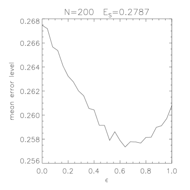
Figure 5: Left panel: “Correlation profile” $c_{\rm a}\left(\phi\right)$ according to Eq. (16) (solid line) and constant value $c_{\rm o}=8$ (dashed line). Right panel: Mean error level for the weighted-average correlation test as a function of the parameter $\varepsilon$ of the weight function (14). The number of galaxies is $N=200$. As in Fig. 4 $E_{\rm S}$ denotes the corresponding result obtained from Spearman’s rank-order test.

4 Data

Now that the weighted average as a method to detect a possible quasar-galaxy associations has been tested numerically, we are going to reanalyze the correlations between 1Jy quasars and IRAS galaxies reported in BS. Because of the high significance of their results it seems promising to try to find additional information such as a correlation scale or amplitude.

4.1 Sample selection

Our investigation is based on exactly the same data set as was used in BS; the reader is referred to this paper for details.

The positions and photometric data of the galaxies are taken from the Infrared Astronomical Satellite (IRAS) Faint Source Catalog, applying the criterion

$$S_{60}^{2}\geq S_{12}\,S_{25}$$

to identify a source as a likely galaxy, where $S_{n}$ denotes the flux at $n$ micron. To exclude very faint as well as very strong nearby sources the sample is then restricted to objects within the range

$$0.3\,\mbox{Jy}\leq S_{60}\leq 1\,\mbox{Jy}\ \ .$$

A sample of quasars is provided by the optically identified fraction of the 1Jy catalog. This catalog contains bright extragalactic radio sources with a 5-GHz flux of above 1 Jy (Kühr et al. [1981], Stickel et al. [1993], Stickel & Kühr [1993a], [1993b]). From the 426 radio sources with known redshift we select different subsamples, each of them characterized by a lower and an upper limit $z_{\rm min}$ and $z_{\rm max}$ of the redshift as well as an upper limit $m_{\rm max}$ of the apparent magnitude.

To perform the statistical analysis we extract from the IRAS catalog a ring-like galaxy field of radii $\phi_{\rm in}$ and $\phi_{\rm out}$ around the position of each of the selected quasars. Merging them as explained in Sec. 2.2 we end up with a total ring-like galaxy field of $N$ galaxies, which can be subjected to the weighted-average correlation test. It has already been pointed out that we assume the galaxies to be distributed independently of one another. In particular this assumption enters the derivation of the optimum weight function and is fundamental for the calculation of any error level given in this paper, because our null-hypothesis is a Poissonian distribution of galaxies. However, the number density of IRAS galaxies is of the order of 1 per square-degree, and the individual galaxy fields are taken from very different positions on the sky. As a consequence, galaxy-galaxy correlations on the merged total field should be negligible.

4.2 Correlation analysis

In order to allow for a direct comparison of our results with those obtained in BS using Spearman’s rank-order test, we first adopt the value of $\phi_{\rm out}=28.21$ arcmin. This radius had been chosen such that the area $\pi\phi_{\rm out}^{2}$ around each of the quasars was $2500$ arcmin², in agreement with an earlier investigation of 1Jy-sources and Lick galaxies by Fugmann ([1990]).

As the IRAS catalog contains a few sources which are located within a few arcseconds from the position of one of the 1Jy-quasars (cf. BS) and can therefore possibly be identified with the corresponding quasars, we remove a small circle from the center of our galaxy fields by setting $\phi_{\rm in}=10$ arcsec.

Tables 1 and 2 summarize the results of the correlation tests. The different columns present the following information: $z_{\rm min}$ denotes the minimum redshift, $z_{\rm max}$ the maximum redshift, $m_{\rm max}$ the maximum apparent magnitude of the selected quasar subsample and $N_{\rm Q}$ the number of quasars within this subsample. The total number of galaxies is $N$ and the two remaining columns display the error levels $\varepsilon_{\rm wa}$ and $\varepsilon_{\rm sp}$ in percent as obtained from the weighted-average and Spearman’s rank-order tests, respectively. The former is derived from a numerical simulation of $10^{6}$ random (Poissonian) galaxy fields, the latter is taken from BS. In Table 1, where no value of $z_{\rm max}$ is given, the subsamples do not have an upper limit of the redshift, i.e. formally it is $z_{\rm max}=\infty$.

Table 1: Results of the correlation tests between 1Jy quasars and IRAS galaxies. The error level (in %) as obtained from the weighted average is denoted by $\varepsilon_{\rm wa}$, whereas $\varepsilon_{\rm sp}$ is the error level from the Spearman’s rank test as reported in BS. The remaining symbols are $z_{\rm min}$ and $m_{\rm max}$ for the minimum redshift and maximum apparent magnitude of the quasar subsample, $N_{\rm Q}$ for the number of quasars, $N$ for the number of galaxies and $\phi_{\rm out}$ denoting the outer radius of the galaxy fields.

			$\phi_{\rm out}=28.21^{\prime}$
$z_{\rm min}$	$m_{\rm max}$	$N_{\rm Q}$	$N$	$\varepsilon_{\rm wa}$	$\varepsilon_{\rm sp}$
0.50	21.00	238	159	.7	23.5
0.50	20.00	218	152	.4	14.1
0.50	19.00	192	141	1.3	20.5
0.50	18.75	169	127	2.3	30.5
0.50	18.50	161	114	2.8	49.3
0.50	18.25	123	89	19.5	30.9
0.50	18.00	114	82	34.5	46.2
0.75	21.00	179	119	2.7	15.9
0.75	20.00	166	113	1.4	16.0
0.75	19.00	144	105	3.7	16.2
0.75	18.75	126	93	8.4	24.4
0.75	18.50	120	84	9.4	29.0
0.75	18.25	87	64	42.1	37.7
0.75	18.00	80	58	67.4	38.2
1.00	21.00	130	90	4.8	32.4
1.00	20.00	123	86	3.1	22.5
1.00	19.00	107	79	8.6	29.3
1.00	18.75	94	70	5.5	17.8
1.00	18.50	88	61	6.0	24.4
1.00	18.25	60	47	52.5	53.8
1.00	18.00	54	43	74.0	73.2
1.25	21.00	97	65	1.0	2.8
1.25	20.00	93	63	.9	4.2
1.25	19.00	80	56	3.1	4.4
1.25	18.75	68	47	1.4	4.7
1.25	18.50	64	46	1.1	6.2
1.25	18.25	42	33	26.6	14.2
1.25	18.00	37	29	48.9	38.2
1.50	21.00	59	33	9.5	0.9
1.50	20.00	56	33	9.5	0.2
1.50	19.00	46	30	5.6	0.7
1.50	18.75	36	23	3.8	0.4
1.50	18.50	34	22	2.9	0.3
1.50	18.25	20	14	7.9	0.2
1.50	18.00	18	14	7.9	1.2

Table 2: As table 1 but for non-overlapping redshift intervals of the quasar subsamples.

				$\phi_{\rm out}=28.21^{\prime}$
$z_{\rm min}$	$z_{\rm max}$	$m_{\rm max}$	$N_{\rm Q}$	$N$	$\varepsilon^{\rm wa}$
0.50	0.75	21.00	61	40	5.3
0.50	0.75	20.00	53	39	4.4
0.50	0.75	19.00	49	36	7.5
0.50	0.75	18.75	44	34	5.0
0.50	0.75	18.50	42	30	5.7
0.50	0.75	18.25	37	25	9.6
0.50	0.75	18.00	35	24	8.7
0.75	1.00	21.00	49	29	14.1
0.75	1.00	20.00	43	27	10.6
0.75	1.00	19.00	37	26	9.9
0.75	1.00	18.75	32	23	49.2
0.75	1.00	18.50	32	23	49.2
0.75	1.00	18.25	27	17	28.7
0.75	1.00	18.00	26	15	38.9
1.00	1.25	21.00	34	25	77.7
1.00	1.25	20.00	31	23	67.6
1.00	1.25	19.00	28	23	67.7
1.00	1.25	18.75	27	23	67.7
1.00	1.25	18.50	25	15	88.7
1.00	1.25	18.25	18	14	88.0
1.00	1.25	18.00	17	14	88.0
1.25	1.50	21.00	38	32	2.2
1.25	1.50	20.00	37	30	1.6
1.25	1.50	19.00	34	26	13.3
1.25	1.50	18.75	32	24	8.1
1.25	1.50	18.50	30	24	8.1
1.25	1.50	18.25	22	19	67.7
1.25	1.50	18.00	19	15	96.3
1.50	$\infty$	21.00	59	33	9.5
1.50	$\infty$	20.00	56	33	9.5
1.50	$\infty$	19.00	46	30	5.6
1.50	$\infty$	18.75	36	23	3.8
1.50	$\infty$	18.50	34	22	2.9
1.50	$\infty$	18.25	20	14	7.9
1.50	$\infty$	18.00	18	14	7.9

A comparison of $\varepsilon_{\rm aw}$ and $\varepsilon_{\rm sp}$ reveals similar properties of the error levels of the weighted average and Spearman’s rank test concerning their dependence on $z_{\rm min}$ and $m_{\rm max}$. However, for subsamples with $z_{\rm min}<1.5$ the weighted average very often yields strikingly lower values of the error level (and thus statistically more significant results) than Spearman’s rank test. This effect becomes even more important if taking into account that the $\varepsilon_{\rm sp}$ have been derived without removing the mentioned IRAS counterparts of the 1Jy quasars from the galaxy fields. Such counterparts can be found in the subsamples with $z_{\rm min}<1$, so the reported values of $\varepsilon_{\rm sp}$ for them are probably too low.

As shown in BS, the IRAS catalog probably extends to galaxy redshifts up to 1. As a consequence there might be a spatial association between IRAS galaxies and 1Jy quasars with a redshift below $z=1$ which, of course, could show up in our correlation tests. Therefore, the quasar subsamples with $z_{\rm min}\geq 1$ are the most interesting ones in the context of gravitational lensing. Table 2 gives a better insight into the dependence of the correlations upon the quasar redshift, because the listed results are based on non-overlapping redshift bins. Surprisingly, we find an anticorrelation for $1.0\leq z<1.25$, but at a significance below $10\%$.

Now we want to investigate the question of how the results are influenced by the choice of the outer radius $\phi_{\rm out}$ of the galaxy fields. As Spearman’s rank test is sensitive to the overall gradient of the galaxy number density over the field, $\phi_{\rm out}$ must be adapted to the angular scale of the expected correlations. But then a low error level can equally be induced by a galaxy overdensity near the center or an underdensity in the outer regions of the field, relative to the mean number density on large scales. Figure 6 shows the distribution of galaxies around 1Jy quasars on fields of radius $1$ deg. Each dot corresponds to one galaxy: The position along the horizontal axis indicates its distance to the quasar, whereas on the vertical axis the quasar redshift can be read off. The quadratic scaling of the horizontal axis assures that a constant galaxy number density on the galaxy fields transforms to a constant number density of dots in the plot. Considering the galaxy distribution around quasars of redshift $z>1.5$, i.e. the dots above the dashed line, one finds that there seems to be a “hole” in the range $0.15<\phi^{2}/\left(1{\rm deg}\right)^{2}<0.25$ which is the outer region of galaxy fields with $\phi_{\rm out}\approx 30$ arcmin. This deficit of galaxies could possibly yield a major contribution to the low error levels recorded in Tables 1 and 2 for $z_{\rm min}=1.5$. To remove that contribution one would like to increase $\phi_{\rm out}$, thereby gaining information about the large scale mean galaxy number density. On the other hand this will decrease the overall density gradient once $\phi_{\rm out}$ becomes larger than the correlation length scale and therefore the significance of the result from Spearman’s rank test will decrease.

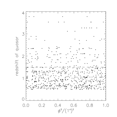
Figure 6: Distribution of IRAS galaxies around 1Jy quasars of redshift $z\geq 0.5$ and apparent visual magnitude $m\leq 21$.

This problem can be overcome with the weighted-average correlation test, if a weight function $g\left(\phi\right)$ like (12) is applied. On the angular scale $\phi\leq\phi_{\rm o}=0.24$ deg the strong dependence of the expected correlations on $\phi$ enables the weighted average to detect a gradient of the galaxy number density. For angular distances $\phi\gg\phi_{\rm o}$ the weight function $g\left(\phi\right)$ is flat. Therefore, in the outer regions not the exact distribution of galaxies but only their mean number density is relevant. This means the weighted average both is sensitive to a quasar-galaxy correlation on a fixed angular radius $\phi_{\rm o}$ and at the same time includes the information on the mean galaxy density from the outer parts of the field. Consequently, and in contrast to Spearman’s rank test, our method can be used to effectively analyse large galaxy fields.

For four different quasar subsamples Fig. 7 displays the error level for rejecting the null-hypothesis of a Poissonian galaxy distribution as a function of the outer field radius $\phi_{\rm out}\leq 2$ deg. The curves illustrate that a relatively small variation of $\phi_{\rm out}$ can have a significant effect on the resulting value of the error level, even if $\phi_{\rm out}$ is beyond 1 deg. Tables 3 and 4 summarize the results obtained by reanalysing all the quasar subsamples as listed in tables 1 and 2 with an outer radius of 2 deg.

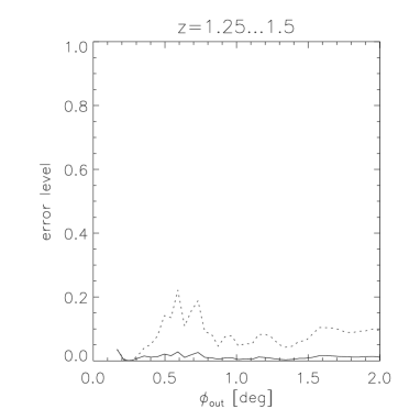
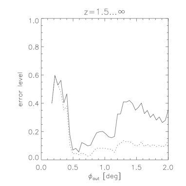
Figure 7: Error level for rejecting the null-hypothesis of a Poissonian galaxy distribution as a function of the outer field radius $\phi_{\rm out}$ for four different quasar subsamples. The redshift range of the quasars is denoted by $z$, their maximum visual magnitude is $m_{\rm max}=21$ for the solid lines and $m_{\rm max}=19$ for the dotted lines.

Table 3: As table 1 but with an outer galaxy field radius of $\phi_{\rm out}=2^{\rm o}$.

			$\phi_{\rm out}=2^{\rm o}$
$z_{\rm min}$	$m_{\rm max}$	$N_{\rm Q}$	$N$	$\varepsilon_{\rm wa}$
0.50	21.00	238	2818	7
0.50	20.00	218	2585	2
0.50	19.00	192	2278	1
0.50	18.75	169	1984	1
0.50	18.50	161	1825	2
0.50	18.25	123	1426	8
0.50	18.00	114	1326	15
0.75	21.00	179	2127	21
0.75	20.00	166	1977	12
0.75	19.00	144	1727	8
0.75	18.75	126	1482	8
0.75	18.50	120	1356	10
0.75	18.25	87	1002	23
0.75	18.00	80	913	37
1.00	21.00	130	1555	19
1.00	20.00	123	1482	15
1.00	19.00	107	1312	15
1.00	18.75	94	1140	7
1.00	18.50	88	1014	9
1.00	18.25	60	703	19
1.00	18.00	54	626	24
1.25	21.00	97	1082	4
1.25	20.00	93	1035	3
1.25	19.00	80	909	5
1.25	18.75	68	745	2
1.25	18.50	64	699	1
1.25	18.25	42	481	9
1.25	18.00	37	417	14
1.50	21.00	59	625	35
1.50	20.00	56	599	30
1.50	19.00	46	507	14
1.50	18.75	36	368	5
1.50	18.50	34	334	3
1.50	18.25	20	203	7
1.50	18.00	18	189	4

Table 4: As table 2 but with an outer galaxy field radius of $\phi_{\rm out}=2^{\rm o}$.

				$\phi_{\rm out}=2^{\rm o}$
$z_{\rm min}$	$z_{\rm max}$	$m_{\rm max}$	$N_{\rm Q}$	$N$	$\varepsilon_{\rm wa}$
0.50	0.75	21.00	61	713	7
0.50	0.75	20.00	53	617	2
0.50	0.75	19.00	49	560	2
0.50	0.75	18.75	44	511	1
0.50	0.75	18.50	42	478	3
0.50	0.75	18.25	37	433	9
0.50	0.75	18.00	35	422	11
0.75	1.00	21.00	49	572	44
0.75	1.00	20.00	43	495	27
0.75	1.00	19.00	37	415	14
0.75	1.00	18.75	32	342	35
0.75	1.00	18.50	32	342	35
0.75	1.00	18.25	27	299	48
0.75	1.00	18.00	26	287	67
1.00	1.25	21.00	34	483	92
1.00	1.25	20.00	31	457	89
1.00	1.25	19.00	28	413	78
1.00	1.25	18.75	27	405	75
1.00	1.25	18.50	25	325	96
1.00	1.25	18.25	18	222	67
1.00	1.25	18.00	17	209	60
1.25	1.50	21.00	38	457	1
1.25	1.50	20.00	37	436	1
1.25	1.50	19.00	34	402	9
1.25	1.50	18.75	32	377	6
1.25	1.50	18.50	30	365	5
1.25	1.50	18.25	22	278	30
1.25	1.50	18.00	19	228	59
1.50	$\infty$	21.00	59	625	35
1.50	$\infty$	20.00	56	599	30
1.50	$\infty$	19.00	46	507	14
1.50	$\infty$	18.75	36	368	5
1.50	$\infty$	18.50	34	334	3
1.50	$\infty$	18.25	20	203	7
1.50	$\infty$	18.00	18	189	4

A more detailed view of the angular galaxy distribution at small distances to 1Jy quasars can be obtained from the correlation functions plotted in Fig. 8. They are calculated using ring-like total galaxy fields of radii $\phi_{\rm in}=10$ arcsec and $\phi_{\rm out}=0.5$ deg constructed according to Sec. 2.2 by merging the individual galaxy fields around the quasars of a given subsample. As before, the inner part is removed to ensure that the fields are not contaminated by the quasars themselves. A total galaxy field is then divided into $n=10$ sub-rings $\left[\varrho_{i},\varrho_{i+1}\right]$ given by Eq. (6). Denoting the number of galaxies within sub-ring no. $i$ by $z_{i}$ and its solid angle by $A_{i}:=\pi\left(\varrho_{i+1}^{2}-\varrho_{i}^{2}\right)$ we derive the value $\xi_{i}$ from

$$\xi_{i}:=\frac{z_{i}\,\sum_{j}A_{j}}{A_{i}\,\sum_{j}z_{j}}-1$$

and assign it to the “mean radius” $\left(\varrho_{i}+\varrho_{i+1}\right)/2$ of the ring.

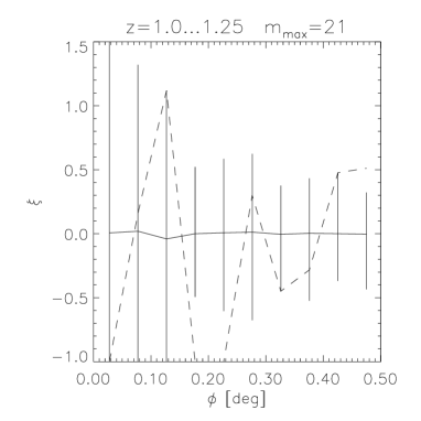
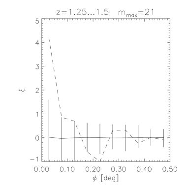
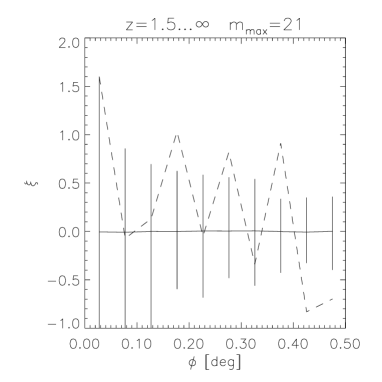
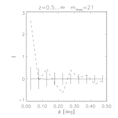
Figure 8: Quasar-galaxy correlation function for 1Jy quasars and IRAS galaxies determined from different quasar subsamples. The redshift range of the quasars is denoted by $z$, their maximum visual magnitude by $m_{\rm max}$.

In the diagrams of Fig. 8 the corresponding points are connected by a dashed line which can be interpreted as an approximation to the quasar-galaxy correlation function. To give an estimate of the errors we do not attach error bars of length $\sqrt{z_{i}}$ to a graph as it is commonly done, because their significance level is strongly dependent on $z_{i}$ if $z_{i}$ is small. Instead we numerically generate a set of 1000 artificial galaxy fields with a random (Poissonian) galaxy distribution. The number of galaxies on each of them is equal to that of the total galaxy field of the regarded quasar subsample. They are subjected to the same procedure as the real fields and for each sub-ring we derive the mean value of $\xi_{i}$ and a $70\%$ error bar: $15\%$ of the simulations yield a value of $\xi_{i}$ below the lower end of the error bar, the values of an equal fraction are above the upper end.

The selected quasar subsamples are characterised in the diagram headings by the redshift $z$ of the quasars and their apparent visual magnitude $m$. The bottom right panel which is calculated from our largest subsample shows a strong signal of a correlation. However, if compared to Fig. 2 the length scale of the correlation appears to be smaller and its amplitude to be much greater than expected from the gravitational lens effect. This is not too surprising, because as it was mentioned above there might be a spatial association between IRAS galaxies and low redshift quasars. The remaining three panels are obtained from three neighbouring high-redshift subsamples. They visualize the results from Table 2: quasar-galaxy anticorrelation for the quasar redshift range $1.0\leq z<1.25$, correlations for $1.25\leq z<1.5$ and $z\geq 1.5$. From the top right diagram it is evident that the correlation for quasars with $1.25\leq z<1.5$ is produced by a significant galaxy overdensity close to the quasars, again with an amplitude greater than expected from the numerical simulations reported by Bartelmann ([1995]), whereas it seems to be caused by a sharp decrease of the galaxy number density at greater distances in the highest redshift subsample. This decrease corresponds to the “hole” in the galaxy distribution which we have already seen in Fig. 6.

4.3 Additional simulations

Given our null-hypothesis of a purely random distribution of galaxies around the 1Jy quasars we have so far quantified our correlation results in terms of the error level. The error level assigned to a value $R$ of the correlation coefficient $r$ has been introduced to be the probability $\varepsilon:=P_{\rm o}\left(r\geq R\right)$ for $r$ to take a value equal to or greater than $R$ for a Poissonian galaxy distribution.

Suppose now we reject the null hypothesis for some of the quasar subsamples, because the associated error level is low. Assuming the quasar-galaxy correlation to be induced by gravitational lensing we would expect it to be described approximately by a correlation function as derived by Bartelmann (see Sec. 2.2), a fit to which we gave in Eq. (11). With this new premise we can then again ask the question: What is the probability $P_{\rm a}\left(r\geq R\right)$ for the correlation coefficient to take a value equal to or greater than $R$ or, equivalently, what is the probability to find an error level equal to or lower than $\varepsilon$.

In order to find an answer we generated a large number of synthetic galaxy fields of radius $\phi_{\rm out}=30^{\prime}$ following the correlation function (11) and containing 100 galaxies each. We subjected them to both Spearman’s rank-order test and the weighted-average correlation test with the optimum weight function (13) ($h=1$). The fraction of simulated fields resulting in an error level equal to or lower than $\varepsilon$ then directly yields the required probability, which is plotted in Fig. 9, left panel, as a function of $\varepsilon$. The solid line presents the result for the weighted-average test, the dashed line for Spearman’s rank test. The dotted line would arise for both correlation tests if the simulated galaxies were distributed randomly; it just reflects the definition of the error level. Repeating the whole procedure with 3000 galaxies per field produces the right panel of Fig. 9.

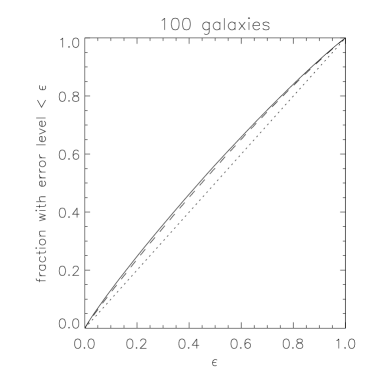
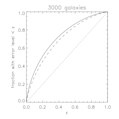
Figure 9: Fraction of simulated galaxy fields yielding an error level equal to or lower than some limit $\varepsilon$ for a galaxy distribution according to the theoretically expected quasar-galaxy correlation analysed with the weighted-average test (solid line) or Spearman’s rank-order test (dashed line) and for a purely random galaxy distribution analysed with either one of the tests (dotted line). The number of galaxies per simulated field is 100 for the left panel and 3000 for the right panel.

As to quasar subsamples with a total number of galaxies $N\approx 100$ on fields of $\phi_{\rm out}\approx 30^{\prime}$ Fig. 9 clearly shows that it is hardly more probable to find low values of the error level in the case of the expected, lensing-induced quasar-galaxy correlation than it is for randomly distributed galaxies. When interpreting this result one should be aware of two facts: On the one hand, $N=100$ is a typical number for rather large quasar subsamples (cf. Tables 1 and 2) and for subsamples with fewer galaxies the difference between the correlated and the random distributions will be even smaller. On the other hand, the correlation function (11) is a fit to what Bartelmann derived from numerical simulations for an artificial galaxy catalog, which includes all galaxies with a visual magnitude $m\leq 21$. Therefore it is quite probable that the IRAS catalog is deeper in redshift than this synthetic catalog and shows a stronger correlation with quasars. Nonetheless, as the curves in Fig. 9 are so extremely close together, we conclude that either

• the low error levels are the result of a statistical fluctuation and do not correspond to a real correlation, or

• the numerical results in Bartelmann ([1995]) significantly underestimate the expected correlations between QSOs and IRAS galaxies, either because the non-linear density inhomogeneities are not properly resolved in these simulations, or because the assumed redshift distribution is much shallower than that of IRAS galaxies, or

• the expected angular scale $\phi_{\rm o}$ is smaller than obtained by Bartelmann, as might be indicated by the correlation function plotted in Fig. 8, or

• for some reason the correlation is not described correctly by assuming a gravitational lensing effect by the large-scale structure. However, in view of the results by Fort et al. ([1995]) quoted in the introduction, we consider this latter possibility unlikely.

5 Summary and conclusions

In this paper, we introduced a new statistical method, the weighted-average correlation test, to look for angular correlations between background quasars and foreground galaxies. As was pointed out by Bartelmann & Schneider, such correlations are predicted by gravitational lens theory under plausible assumptions concerning the quasar luminosity function and the dependence between the distributions of dark and luminous matter.

Whereas the methods applied in earlier investigations of this phenomenon need to group the galaxies according to their positions into some arbitrarily defined bins, the weighted average uses the exact distance of each individual galaxy to the corresponding quasar. Furthermore, if additional information about the assumed correlation is available it can be included into our test via choosing a proper weight function. In an analytic calculation we could derive a formula which allows to construct an optimum weight function from the expected quasar-galaxy correlation function. The verification of this result by means of numerical simulations has also shown that the weighted-average correlation test can be more significant than Spearman’s rank-order test, even if the weight function deviates considerably from its optimum.

To look for a quasar-galaxy correlation we analysed the distribution of IRAS galaxies on circular fields around 1Jy quasars. This was carried out for different quasar subsamples by merging the individual galaxy fields and subjecting the resulting total field to the weighted-average test. As we have explained and illustrated, the tests should be performed on galaxy fields as large as possible. Actually, the outer regions carry useful information about the mean galaxy number density, which is obviously needed to detect a possible galaxy overdensity in the center of the fields. Supplied with an appropriate weight function the weighted average can make use of this information.

With small galaxy fields of radius $\phi_{\rm out}\approx 0.5$ deg as well as with large ones of radius $\phi_{\rm out}=2$ deg many of the quasar subsamples give rise to a low error level for the rejection of a purely random galaxy distribution. This is in agreement with previous findings in BS. As argued there, a correlation of galaxies with low-redshift quasars might be due to a spatial association, whereas a correlation with high-redshift quasars could be caused by gravitational lensing. Nevertheless there seems to be an anticorrelation between galaxies and quasars of redshift $1.0\leq z<1.25$, and its interpretation in terms of these hypotheses is not obvious. However, it should be pointed out that this anticorrelation occurs with an error level larger than 10% and is therefore not of high significance. To visualize the angular galaxy distribution within different subsamples we compiled plots of the quasar-galaxy correlation function. Although they look quite different, this is, of course, not a statistically significant indication that they do not represent realisations of the same parent distribution.

From additional simulations we expected to get further hints for the interpretation of our results. We numerically generated a large number of synthetic galaxy fields with galaxies distributed according to the correlation function expected from gravitational lensing by the large-scale structure as studied in Bartelmann ([1995]). On the basis of these results, we found that the lensing-induced correlations between 1Jy quasars and IRAS galaxies should be detectable neither with the weighted-average test nor with Spearman’s rank-order test, because of the sparseness of the samples.

Therefore, as stated above, we conclude that either

• the low error levels are the result of a statistical fluctuation and do not correspond to a real correlation, or

• the numerical results in Bartelmann ([1995]) significantly underestimate the expected correlations between QSOs and IRAS galaxies, either because the non-linear density inhomogeneities are not properly resolved in these simulations, or because the assumed redshift distribution is much shallower than that of IRAS galaxies, or

• the expected angular scale $\phi_{\rm o}$ is smaller than obtained by Bartelmann, as might be indicated by the correlation function plotted in Fig. 8, or

• for some reason the correlation is not described correctly by assuming a gravitational lensing effect by the large-scale structure. However, in view of the results by Fort et al. ([1995]) quoted in the introduction, we consider this latter possibility unlikely.

Acknowledgements. This work was supported by the “Sonderforschungsbereich 375-95 für Astro–Teilchenphysik” der Deutschen Forschungsgemeinschaft.

Appendix A. Optimizing the weight function

In Sect. 2.1 it was argued that the correlation coefficient $r$ as defined in (2) can be optimized for distinguishing between two statistical hypotheses via maximizing $\left|Q_{1}\right|$, given by Eq. (4). Here we intend to carry out the maximisation for

$$r_{g}\left(\phi_{1},\ldots,\phi_{N}\right):=\frac{1}{N}\sum_{j=1}^{N}g\left(\phi_{j}\right)\ \ ,$$ (17)

which was shown in Sect. 2.2 to be a limiting case of $r$ applied to the analysis of quasar-galaxy correlations. Accordingly, the symbols $\phi_{1},\ldots,\phi_{N}$ denote galaxy positions.

In addition, it will be demonstrated that the weight function $g\left(\phi\right)$ we find in this way also represents nearly a stationary point of the mean error level (3), provided the two hypotheses are “similar”.

We assume the galaxy positions to be independent of one another, so their distribution can be characterised by a one-dimensional radial probability density $p\left(\phi\right)$. Let $p_{\rm o}\left(\phi\right)$ describe the radial galaxy distribution of the null-hypothesis, i.e. without any quasar-galaxy association. Furthermore, suppose we have some hints, e.g. from theory, that the real distribution of galaxies might be represented by the different probability density $p_{\rm a}\left(\phi\right)$. Following Sect. 2.2 we introduce a geometrical factor $G\left(\phi\right)\geq 0$ and write

$$\begin{array}[]{rcll}p_{\rm o}\left(\phi\right)&=&c_{\rm o}\cdot G\left(\phi\right)\ \ ,&\displaystyle\int_{\phi_{\rm in}}^{\phi_{\rm out}}c_{\rm o}\,G\left(\phi\right){\rm d}\phi=1\ \ ,\vspace{1\jot}\\ p_{\rm a}\left(\phi\right)&=&c_{\rm a}\left(\phi\right)\cdot G\left(\phi\right)\ \ ,&\displaystyle\int_{\phi_{\rm in}}^{\phi_{\rm out}}c_{\rm a}\left(\phi\right)G\left(\phi\right){\rm d}\phi=1\ \ .\end{array}$$

A.1  The quantity $Q_{1}$

Using the above expressions we have

$$\left\langle r_{g}\right\rangle_{\rm o} = \int_{\phi_{\rm in}}^{\phi_{\rm out}}\!\cdots\!\int_{\phi_{\rm in}}^{\phi_{\rm out}}\left[\frac{1}{N}\sum_{i=1}^{N}g\left(\phi_{i}\right)\right]\prod_{j=1}^{N}\left[c_{\rm o}\,G\left(\phi_{j}\right){\rm d}\phi_{j}\right]=c_{\rm o}\,\int_{\phi_{\rm in}}^{\phi_{\rm out}}g\left(\phi\right)G\left(\phi\right){\rm d}\phi\ \ ,$$

$$\left\langle r_{g}\right\rangle_{\rm a} = \int_{\phi_{\rm in}}^{\phi_{\rm out}}g\left(\phi\right)c_{\rm a}\left(\phi\right)G\left(\phi\right){\rm d}\phi\ \ ,$$

$$\sigma_{\rm o}^{2} = \int_{\phi_{\rm in}}^{\phi_{\rm out}}\!\cdots\!\int_{\phi_{\rm in}}^{\phi_{\rm out}}\left[r_{g}\left(\phi_{1},\ldots,\phi_{N}\right)-\left\langle r_{g}\right\rangle_{\rm o}\right]^{2}\prod_{j=1}^{N}\left[c_{\rm o}\,G\left(\phi_{j}\right){\rm d}\phi_{j}\right]=$$

$$= \int_{\phi_{\rm in}}^{\phi_{\rm out}}\!\cdots\!\int_{\phi_{\rm in}}^{\phi_{\rm out}}\left[\frac{1}{N}\sum_{i=1}^{N}g\left(\phi_{i}\right)\right]^{2}\prod_{j=1}^{N}\left[c_{\rm o}\,G\left(\phi_{j}\right){\rm d}\phi_{j}\right]-\left\langle r_{g}\right\rangle_{\rm o}^{2}=$$

$$= \frac{1}{N^{2}}\sum_{i=1}^{N}\int_{\phi_{\rm in}}^{\phi_{\rm out}}\left[g\left(\phi_{i}\right)\right]^{2}c_{\rm o}\,G\left(\phi_{i}\right){\rm d}\phi_{i}+$$

$$+\frac{1}{N^{2}}\sum_{{\scriptstyle i,j=1}\atop{\scriptstyle i\neq j}}^{N}\int_{\phi_{\rm in}}^{\phi_{\rm out}}\!\!\int_{\phi_{\rm in}}^{\phi_{\rm out}}g\left(\phi_{i}\right)g\left(\phi_{j}\right)c_{\rm o}^{2}G\left(\phi_{i}\right)G\left(\phi_{j}\right){\rm d}\phi_{i}\,{\rm d}\phi_{j}-\left\langle r_{g}\right\rangle_{\rm o}^{2}=$$

$$= \frac{1}{N}\int_{\phi_{\rm in}}^{\phi_{\rm out}}\left[g\left(\phi\right)\right]^{2}c_{\rm o}\,G\left(\phi\right){\rm d}\phi-\frac{1}{N}\,\left\langle r_{g}\right\rangle_{\rm o}^{2}\ \ .$$

The substitution of $r$ by $r_{g}$ in definition (4) then yields

$$Q_{1} = \sqrt{N}\frac{\int g\left(\phi\right)c_{\rm a}\left(\phi\right)G\left(\phi\right){\rm d}\phi-\int g\left(\phi\right)c_{\rm o}G\left(\phi\right){\rm d}\phi}{\sqrt{\int\left[g\left(\phi\right)\right]^{2}c_{\rm o}G\left(\phi\right){\rm d}\phi-\left[\int g\left(\phi\right)c_{\rm o}G\left(\phi\right){\rm d}\phi\right]^{2}}}=$$ (19)

$$= \int\frac{g\left(\phi^{\prime}\right)-\int g\left(\phi\right)c_{\rm o}G\left(\phi\right){\rm d}\phi}{\sqrt{\int\left[g\left(\phi\right)\right]^{2}c_{\rm o}G\left(\phi\right){\rm d}\phi-\left[\int g\left(\phi\right)c_{\rm o}G\left(\phi\right){\rm d}\phi\right]^{2}}}\sqrt{N}\,c_{\rm a}\left(\phi^{\prime}\right)G\left(\phi^{\prime}\right){\rm d}\phi^{\prime}=$$

$$= \int L\left(\phi,E,W;g\left(\phi\right)\right){\rm d}\phi\ \ ,$$

where all the integrations are to be performed over the interval $\left[\phi_{\rm in},\phi_{\rm out}\right]$ and we have introduced the abbreviations

$$L\left(\phi,E,W;g\left(\phi\right)\right):=\sqrt{N}\,c_{\rm a}\left(\phi\right)G\left(\phi\right)\,\frac{g\left(\phi\right)-E}{\sqrt{W-E^{2}}}\ \ ,$$

$$E := \int_{\phi_{\rm in}}^{\phi_{\rm out}}g\left(\phi\right)c_{\rm o}\,G\left(\phi\right){\rm d}\phi\ \ ,$$

$$W := \int_{\phi_{\rm in}}^{\phi_{\rm out}}\left[g\left(\phi\right)\right]^{2}c_{\rm o}\,G\left(\phi\right){\rm d}\phi\ \ .$$

In order to maximize $\left|Q_{1}\right|$ we investigate the influence of a variation $\varepsilon\cdot h\left(\phi\right)$ of $g\left(\phi\right)$. For that purpose, we substitute $g\left(\phi\right)\rightarrow\gamma\left(\phi,\varepsilon\right):=g\left(\phi\right)+\varepsilon\cdot h\left(\phi\right)$ and find

$$Q_{1}\left(\varepsilon\right)=\int_{\phi_{\rm in}}^{\phi_{\rm out}}L\Bigl{(}\phi,E\left(\varepsilon\right),W\left(\varepsilon\right);\gamma\left(\phi,\varepsilon\right)\Bigr{)}{\rm d}\phi$$

with

$$E\left(\varepsilon\right) := \int_{\phi_{\rm in}}^{\phi_{\rm out}}\gamma\left(\phi,\varepsilon\right)c_{\rm o}\,G\left(\phi\right){\rm d}\phi\ \ ,$$

$$W\left(\varepsilon\right) := \int_{\phi_{\rm in}}^{\phi_{\rm out}}\left[\gamma\left(\phi,\varepsilon\right)\right]^{2}c_{\rm o}\,G\left(\phi\right){\rm d}\phi\ \ .$$

The condition for the weight function $g\left(\phi\right)$ to produce an extreme value of $Q_{1}$ can now be expressed as

$$\left.\frac{{\rm d}}{{\rm d}\varepsilon}Q_{1}\left(\varepsilon\right)\right|_{\varepsilon=0}=\int_{\phi_{\rm in}}^{\phi_{\rm out}}\left.\frac{{\rm d}}{{\rm d}\varepsilon}L\Bigl{(}\phi,E\left(\varepsilon\right),W\left(\varepsilon\right);\gamma\left(\phi,\varepsilon\right)\Bigr{)}\right|_{\varepsilon=0}{\rm d}\phi=0\ \ ,$$ (20)

which is equivalent to

$$\int\left.\frac{\partial L}{\partial\gamma}\left(\phi\right)\right|_{\varepsilon=0}h\left(\phi\right){\rm d}\phi\ +\int\!\!\int\left.\frac{\partial L}{\partial E}\left(\phi\right)\right|_{\varepsilon=0}h\left(t\right)c_{\rm o}\,G\left(t\right){\rm d}t{\rm d}\phi\ +$$ (21)

$$+\ \int\!\!\int\left.\frac{\partial L}{\partial W}\left(\phi\right)\right|_{\varepsilon=0}2\,g\left(t\right)h\left(t\right)c_{\rm o}\,G\left(t\right){\rm d}t{\rm d}\phi=0\ \ ,$$

because of the relations

$$\frac{{\rm d}L}{{\rm d}\varepsilon}=\frac{\partial L}{\partial\gamma}\frac{{\rm d}\gamma\left(\phi,\varepsilon\right)}{{\rm d}\varepsilon}+\frac{\partial L}{\partial E}\frac{{\rm d}E\left(\varepsilon\right)}{{\rm d}\varepsilon}+\frac{\partial L}{\partial W}\frac{{\rm d}W\left(\varepsilon\right)}{{\rm d}\varepsilon}\ \ ,\\$$

and

$$\left.\frac{{\rm d}\gamma\left(\phi,\varepsilon\right)}{{\rm d}\varepsilon}\right|_{\varepsilon=0} = h\left(\phi\right)\ \ ,$$

$$\left.\frac{{\rm d}E\left(\varepsilon\right)}{{\rm d}\varepsilon}\right|_{\varepsilon=0} = \int_{\phi_{\rm in}}^{\phi_{\rm out}}h\left(\phi\right)c_{\rm o}\,G\left(\phi\right){\rm d}\phi\ \ ,$$

$$\left.\frac{{\rm d}W\left(\varepsilon\right)}{{\rm d}\varepsilon}\right|_{\varepsilon=0} = 2\cdot\int_{\phi_{\rm in}}^{\phi_{\rm out}}g\left(\phi\right)h\left(\phi\right)c_{\rm o}\,G\left(\phi\right){\rm d}\phi\ \ .$$

Exchanging both the order of integrations and the variables $\phi$ and $t$ in the second and third term of Eq. (21) leads to

$$\int\left.\frac{\partial L}{\partial\gamma}\left(\phi\right)\right|_{\varepsilon=0}h\left(\phi\right){\rm d}\phi\ +\int\!\!\int\left.\frac{\partial L}{\partial E}\left(t\right)\right|_{\varepsilon=0}h\left(\phi\right)c_{\rm o}\,G\left(\phi\right){\rm d}t{\rm d}\phi\ +$$ (22)

$$+\ \int\!\!\int\left.\frac{\partial L}{\partial W}\left(t\right)\right|_{\varepsilon=0}2g\left(\phi\right)h\left(\phi\right)c_{\rm o}\,G\left(\phi\right){\rm d}t{\rm d}\phi=\int_{\phi_{\rm in}}^{\phi_{\rm out}}q\left(\phi\right)h\left(\phi\right){\rm d}\phi=0\ \ ,$$

where $q\left(\phi\right)$ is defined to be

$$q\left(\phi\right):=\left.\frac{\partial L}{\partial\gamma}\left(\phi\right)\right|_{\varepsilon=0}+c_{\rm o}\,G\left(\phi\right)\int\left.\frac{\partial L}{\partial E}\left(t\right)\right|_{\varepsilon=0}{\rm d}t+2g\left(\phi\right)c_{\rm o}\,G\left(\phi\right)\int\left.\frac{\partial L}{\partial W}\left(t\right)\right|_{\varepsilon=0}{\rm d}t\ \ .$$

As Eq. (22) must hold for an arbitrary choice of $h\left(\phi\right)$, Eq. (20) is finally reduced to

$$q\left(\phi\right)\equiv 0\ \ \ \mbox{on}\ \phi\in\left[\phi_{\rm in},\phi_{\rm out}\right]\ \ .$$

The partial derivatives of $L$ that enter $q$ are

$$\left.\frac{\partial L}{\partial\gamma}\left(\phi\right)\right|_{\varepsilon=0} = \sqrt{N}\cdot\frac{c_{\rm a}\left(\phi\right)G\left(\phi\right)}{\sqrt{W-E^{2}}}\ \ ,$$

$$\left.\frac{\partial L}{\partial E}\left(\phi\right)\right|_{\varepsilon=0} = \sqrt{N}\cdot c_{\rm a}\left(\phi\right)G\left(\phi\right)\left[E\cdot\frac{g\left(\phi\right)-E}{\sqrt{\left(W-E^{2}\right)^{3}}}-\frac{1}{\sqrt{W-E^{2}}}\right]\ \ ,$$

$$\left.\frac{\partial L}{\partial W}\left(\phi\right)\right|_{\varepsilon=0} = -\frac{1}{2}\,\sqrt{N}\cdot c_{\rm a}\left(\phi\right)G\left(\phi\right)\cdot\frac{g\left(\phi\right)-E}{\sqrt{\left(W-E^{2}\right)^{3}}}\ \ ,$$

so after dividing by $\sqrt{N/\left(W-E^{2}\right)}$ we have

$$c_{\rm a}\left(\phi\right)G\left(\phi\right)+c_{\rm o}\,G\left(\phi\right)E\cdot\frac{\int g\left(t\right)c_{\rm a}\left(t\right)G\left(t\right){\rm d}t-E}{W-E^{2}}-$$

$$- c_{\rm o}\,G\left(\phi\right)-c_{\rm o}\,G\left(\phi\right)g\left(\phi\right)\frac{\int g\left(t\right)c_{\rm a}\left(t\right)G\left(t\right){\rm d}t-E}{W-E^{2}}\equiv 0\ \ .$$

We first note that, if $G\left(\phi^{\prime}\right)=0$ at a position $\phi^{\prime}$, this condition is fulfilled for an arbitrary finite value of $g\left(\phi^{\prime}\right)$, whereas for $G\left(\phi\right)\neq 0$ a division by $c_{\rm o}\,G\left(\phi\right)$ yields

$$\frac{c_{\rm a}\left(\phi\right)}{c_{\rm o}}+E\cdot\frac{\int g\left(t\right)c_{\rm a}\left(t\right)G\left(t\right){\rm d}t-E}{W-E^{2}}-1-g\left(\phi\right)\frac{\int g\left(t\right)c_{\rm a}\left(t\right)G\left(t\right){\rm d}t-E}{W-E^{2}}\equiv 0\ \ .$$ (23)

Furthermore, it is easy to see that relation (23) is invariant under linear transformations

$$g\left(\phi\right)\rightarrow\widetilde{g}\left(\phi\right):=\alpha\,g\left(\phi\right)+\beta\ \ ,\ \ \ \alpha\neq 0\ \ ,$$

because

$$E \rightarrow \widetilde{E}:=\int\widetilde{g}\left(\phi\right)c_{\rm o}\,G\left(\phi\right){\rm d}\phi=\alpha\,E+\beta\ \ ,$$

$$W \rightarrow \widetilde{W}:=\int\left[\widetilde{g}\left(\phi\right)\right]^{2}c_{\rm o}\,G\left(\phi\right){\rm d}\phi=\alpha^{2}W+2\alpha\beta E+\beta^{2}\ \$$

and

$$\widetilde{E}^{2}=\alpha^{2}E^{2}+2\alpha\beta E+\beta^{2}\ \ ,$$

$$\widetilde{W}-\widetilde{E}^{2}=\alpha^{2}\left(W-E^{2}\right)\ \ ,$$

$$\int\widetilde{g}\left(t\right)c_{\rm a}\left(t\right)G\left(t\right){\rm d}t-\widetilde{E}=\alpha\left[\int g\left(t\right)c_{\rm a}\left(t\right)G\left(t\right){\rm d}t-E\right]\ \ .$$

As a consequence, we can chose $\widetilde{g}\left(\phi\right)$ such that

$$\frac{\int\widetilde{g}\left(t\right)c_{\rm a}\left(t\right)G\left(t\right){\rm d}t-\widetilde{E}}{\widetilde{W}-\widetilde{E}^{2}}=1\ \ \wedge\ \ \widetilde{E}=1\ \ ,$$

thereby simplifying (23) to

$$\widetilde{g}\left(\phi\right)=c_{\rm a}\left(\phi\right)/c_{\rm o}\ \ .$$

From this we derive the stationary points of $Q_{1}$ with respect to the weight function $g\left(\phi\right)$ to be given by

$$g\left(\phi\right)=ac_{\rm a}\left(\phi\right)+b\ \ ,$$ (24)

with arbitrary constants $a\neq 0$ and $b$.

The next step of our calculation is to show that the stationary point given by relation (24) specifies a local maximum of $\left|Q_{1}\right|$. We consider an arbitrary deviation $\varepsilon\cdot h\left(\phi\right)$ of $g\left(\phi\right)$ from (24),

$$\gamma\left(\phi,\varepsilon\right):=a\cdot\left[c_{\rm a}\left(\phi\right)+\varepsilon\cdot h\left(\phi\right)\right]+b\ \ ,$$ (25)

and analyse its effect on $Q_{1}$:

$$Q_{1}\left(\varepsilon\right):=\frac{\int\gamma\left(\phi,\varepsilon\right)c_{\rm a}\left(\phi\right)G\left(\phi\right){\rm d}\phi-\int\gamma\left(\phi,\varepsilon\right)c_{\rm o}\,G\left(\phi\right){\rm d}\phi}{\sqrt{\int\left[\gamma\left(\phi,\varepsilon\right)-\int\gamma\left(t,\varepsilon\right)c_{\rm o}\,G\left(t\right){\rm d}t\right]^{2}c_{\rm o}\,G\left(\phi\right){\rm d}\phi}}\ \ .$$

The denominator on the right hand side of this expression is equal to zero at some point $\varepsilon=\varepsilon^{\prime}$ only if

$$\gamma\left(\phi,\varepsilon^{\prime}\right)=\int\gamma\left(t,\varepsilon^{\prime}\right)c_{\rm o}\,G\left(t\right){\rm d}t\ \ ,$$

which is equivalent to $\gamma(\phi,\varepsilon^{\prime})$ being a constant in $\phi$. That, in turn, requires $h\left(\phi\right)=-(1/\varepsilon^{\prime})c_{\rm a}\left(\phi\right)+\mbox{const}$, resulting in

$$\gamma\left(\phi,\varepsilon\right)=\alpha\left(\varepsilon\right)c_{\rm a}\left(\phi\right)+\beta\left(\varepsilon\right)\ \ ,$$ (26)

where $\alpha\left(\varepsilon\right)$ and $\beta\left(\varepsilon\right)$ are constants in $\phi$. Equation (26), however, implies $\left|Q_{1}\left(\varepsilon\right)\right|=\mbox{const}$, as can easily be derived from the definition of $Q_{1}\left(\varepsilon\right)$. In the subsequent investigation we will therefore, without loss of generality, exclude the case of a vanishing denominator of $Q_{1}\left(\varepsilon\right)$.

Introducing new abbreviations

$$X := \int\left[h\left(\phi\right)-\int h\left(t\right)c_{\rm o}\,G\left(t\right){\rm d}t\right]^{2}G\left(\phi\right){\rm d}\phi=$$

$$= \int\left[h\left(\phi\right)\right]^{2}G\left(\phi\right){\rm d}\phi-c_{\rm o}\left[\int h\left(t\right)G\left(t\right){\rm d}t\right]^{2}\geq 0\ \ ,$$

$$Y := \int h\left(\phi\right)c_{\rm a}\left(\phi\right)G\left(\phi\right){\rm d}\phi-\int h\left(\phi\right)c_{\rm o}\,G\left(\phi\right){\rm d}\phi=$$

$$= \int\left[h\left(\phi\right)-\int h\left(t\right)c_{\rm o}\,G\left(t\right){\rm d}t\right]\bigl{[}c_{\rm a}\left(\phi\right)-c_{\rm o}\bigr{]}G\left(\phi\right){\rm d}\phi\ \ ,$$

$$Z := \int\left[c_{\rm a}\left(\phi\right)\right]^{2}G\left(\phi\right){\rm d}\phi-\int c_{\rm a}\left(\phi\right)c_{\rm o}\,G\left(\phi\right){\rm d}\phi=$$

$$= \int\left[c_{\rm a}\left(\phi\right)\right]^{2}G\left(\phi\right){\rm d}\phi-c_{\rm o}=\int\left[c_{\rm a}\left(\phi\right)-c_{\rm o}\right]^{2}G\left(\phi\right){\rm d}\phi\geq 0\ \ ,$$

and

$$q_{1}\left(\varepsilon\right):=\frac{Z+\varepsilon Y}{\sqrt{c_{\rm o}Z+2\varepsilon c_{\rm o}Y+\varepsilon^{2}c_{\rm o}X}}$$ (27)

we write $Q_{1}\left(\varepsilon\right)$ in the form

$$Q_{1}\left(\varepsilon\right)=\frac{a}{\left|a\right|}\,q_{1}\left(\varepsilon\right)\ \ .$$

The first derivative of $q_{1}\left(\varepsilon\right)$ in $\varepsilon$ is

$$\frac{{\rm d}}{{\rm d}\varepsilon}\,q_{1}\left(\varepsilon\right)=\varepsilon\cdot\frac{c_{\rm o}Y^{2}-c_{\rm o}XZ}{\left(c_{\rm o}Z-2\varepsilon c_{\rm o}Y+\varepsilon^{2}c_{\rm o}X\right)^{3/2}}\ \ ,$$

where, because of the Schwarz inequality, the numerator on the right hand side is always lower than or equal to zero. This means $q_{1}\left(\varepsilon\right)$ is monotonously increasing for $\varepsilon<0$ but monotonously decreasing for $\varepsilon>0$. Accordingly, $q_{1}\left(\varepsilon\right)$ takes its global maximum at $\varepsilon=0$ which is, as $q_{1}\left(\varepsilon=0\right)\geq 0$ and $\left|Q_{1}\left(\varepsilon\right)\right|=\left|q_{1}\left(\varepsilon\right)\right|$, at least a local maximum of $\left|Q_{1}\left(\varepsilon\right)\right|$.

At this point we know condition (24) to correspond to a local maximum of $\left|Q_{1}\right|$. The final goal of the following arguments is to demonstrate that this local maximum is also the global maximum. Taking into account that $\left|Q_{1}\left(\varepsilon\right)\right|=\left|q_{1}\left(\varepsilon\right)\right|$ and that the global maximum of $q_{1}\left(\varepsilon\right)$ is located at $\varepsilon=0$ with $q_{1}\left(0\right)\geq 0$ it is sufficient to prove $|q_{1}^{*}|\leq q_{1}\left(0\right)$ for the absolute minimum $q_{1}^{*}$ of $q_{1}\left(\varepsilon\right)$. Because of the monotony of $q_{1}\left(\varepsilon\right)$ we obtain

$$q_{1}^{*}={\rm min}\left\{\lim_{\varepsilon\to-\infty}q_{1}\left(\varepsilon\right),\lim_{\varepsilon\to\infty}q_{1}\left(\varepsilon\right)\right\}\ \ ,$$

with

$$\lim_{\varepsilon\to\infty}q_{1}\left(\varepsilon\right)=-\lim_{\varepsilon\to-\infty}q_{1}\left(\varepsilon\right)=Y/\sqrt{X}\ \ ,$$

as can be seen from definition (27). Depending on the sign of $Y$ one of the limits is greater than or equal to zero but lower than or equal to $q_{1}\left(0\right)$, because $q_{1}\left(0\right)$ is the absolute maximum of $q_{1}\left(\varepsilon\right)$. Therefore, it is

$$q_{1}\left(0\right)\geq\left|\lim_{\varepsilon\to\infty}q_{1}\left(\varepsilon\right)\right|=\left|\lim_{\varepsilon\to-\infty}q_{1}\left(\varepsilon\right)\right|=\left|q_{1}^{*}\right|\ \ ,$$

which means $\left|Q_{1}\right|$ is globally maximized if the weight function $g\left(\phi\right)$ of the correlation coefficient (17) is in agreement with Eq. (24).

A.2  The mean error level

In analogy to Eq. (3) one can define the mean error level $\left\langle P_{\rm o}\left(r_{g}\geq R\right)\right\rangle$ of the correlation coefficient $r_{g}$. A good distinction between the two galaxy distributions described by $p_{\rm o}\left(\phi\right)$ and $p_{\rm a}\left(\phi\right)$ is possible if the mean error level is low. Therefore, we would like the weight function $g\left(\phi\right)$ to minimize $\left\langle P_{\rm o}\left(r_{g}\geq R\right)\right\rangle$. For this it is a necessary condition that the mean error level is stationary with respect to small variations $\varepsilon\cdot h\left(\phi\right)$ of $g\left(\phi\right)$:

$$\left.\frac{{\rm d}}{{\rm d}\varepsilon}\left\langle P_{\rm o}\left(r_{\gamma}\geq R\right)\right\rangle\right|_{\varepsilon=0}=0\ \ ,$$ (28)

with $\gamma\left(\phi,\varepsilon\right):=g\left(\phi\right)+\varepsilon\,h\left(\phi\right)$. If we write $p_{\rm a}\left(\phi\right)$ in the form

$$p_{\rm a}\left(\phi\right):=p_{\rm o}\left(\phi\right)\left(1+\eta\,\nu\left(\phi\right)\right)$$

and fix $\nu\left(\phi\right)$, then in general $g\left(\phi\right)$ will depend on $\eta$. But as (28) must hold for any value of $\eta$, we have

$$\left.\frac{\partial}{\partial\eta}\frac{\partial}{\partial\varepsilon}\left\langle P_{\rm o}\left(r_{\gamma}\geq R\right)\right\rangle\right|_{\varepsilon=0}=0\ \ .$$ (29)

What we want to prove here is that for $\eta\to 0$ both Eq. (28) and Eq. (29) hold if $g\left(\phi\right)$ is in agreement with Eq. (24). For convenience, let us define the symbols

$$P_{{\rm o}g}\left(R\right) := 1-P_{\rm o}\left(r_{g}\geq R\right)=P_{\rm o}\left(r_{g}<R\right)=$$

$$= \int\!\!\cdots\!\!\int p_{\rm o}\left(\phi_{1}\right)\cdots p_{\rm o}\left(\phi_{N}\right)\,\theta\left(R-\frac{1}{N}\sum_{i=1}^{N}g\left(\phi_{i}\right)\right)\,{\rm d}^{N}\phi\ \ ,$$

$$P_{{\rm a}g}\left(R\right) := P_{\rm a}\left(r_{g}<R\right)=\int\!\!\cdots\!\!\int p_{\rm a}\left(\phi_{1}\right)\cdots p_{\rm a}\left(\phi_{N}\right)\,\theta\left(R-\frac{1}{N}\sum_{i=1}^{N}g\left(\phi_{i}\right)\right)\,{\rm d}^{N}\phi\ \ ,$$

$$p_{{\rm o}g}\left(r\right) := \frac{{\rm d}}{{\rm d}r}P_{{\rm o}g}\left(r\right)=\int\!\!\cdots\!\!\int p_{\rm o}\left(\phi_{1}\right)\cdots p_{\rm o}\left(\phi_{N}\right)\,\delta\left(r-\frac{1}{N}\sum_{i=1}^{N}g\left(\phi_{i}\right)\right)\,{\rm d}^{N}\phi\ \ ,$$

$$p_{{\rm a}g}\left(r\right) := \frac{{\rm d}}{{\rm d}r}P_{{\rm a}g}\left(r\right)=\int\!\!\cdots\!\!\int p_{\rm a}\left(\phi_{1}\right)\cdots p_{\rm a}\left(\phi_{N}\right)\,\delta\left(r-\frac{1}{N}\sum_{i=1}^{N}g\left(\phi_{i}\right)\right)\,{\rm d}^{N}\phi\ \ ,$$

with Dirac’s delta function $\delta\left(r\right)$ and Heaviside’s step function $\theta\left(r\right)$. All the integrations have to be performed over $\left[\phi_{\rm in},\phi_{\rm out}\right]$. A partial integration of the mean error level yields

$$\left\langle P_{{\rm o}\gamma}\left(r_{\gamma}\geq r\right)\right\rangle=1-\int_{-\infty}^{\infty}P_{{\rm o}\gamma}\left(r\right)p_{{\rm a}\gamma}\left(r\right)\,{\rm d}r=\int_{-\infty}^{\infty}P_{{\rm a}\gamma}\left(r\right)p_{{\rm o}\gamma}\left(r\right)\,{\rm d}r\ \ .$$

It is evident that for $\eta\to 0$ the mean error level reaches the constant value $\left\langle P_{{\rm o}\gamma}\left(r_{\gamma}\geq r\right)\right\rangle=\int P_{{\rm o}g}\left(r\right)p_{{\rm o}g}\left(r\right)\,{\rm d}r=1/2$ for an arbitrary weight function $g$, so obviously Eq. (28) is fulfilled. Furthermore, we find

$$\left.\frac{\partial}{\partial\eta}\frac{\partial}{\partial\varepsilon}\left\langle P_{{\rm o}\gamma}\left(r_{\gamma}\geq r\right)\right\rangle\right|_{\varepsilon=0\atop\eta=0}=\left.\int\frac{\partial}{\partial\eta}\left[p_{{\rm o}\gamma}\left(r\right)\frac{\partial}{\partial\varepsilon}P_{{\rm a}\gamma}\left(r\right)+P_{{\rm a}\gamma}\left(r\right)\frac{\partial}{\partial\varepsilon}p_{{\rm o}\gamma}\left(r\right)\right]{\rm d}r\right|_{\varepsilon=0\atop\eta=0}=$$

$$= \left.\int\frac{\partial}{\partial\eta}\left[p_{{\rm o}\gamma}\left(r\right)\frac{\partial}{\partial\varepsilon}P_{{\rm a}\gamma}\left(r\right)-p_{{\rm a}\gamma}\left(r\right)\frac{\partial}{\partial\varepsilon}P_{{\rm o}\gamma}\left(r\right)\right]{\rm d}r\right|_{\varepsilon=0\atop\eta=0}=$$

$$= \frac{1}{N}\int\!\!\cdots\!\!\int p_{\rm o}\left(\phi_{1}\right)\cdots p_{\rm o}\left(\phi_{N}\right)\,p_{\rm o}\left(\phi_{1}^{\prime}\right)\cdots p_{\rm o}\left(\phi_{N}^{\prime}\right)\,\delta\left(\frac{1}{N}\sum_{i=1}^{N}g\left(\phi_{i}\right)-\frac{1}{N}\sum_{j=1}^{N}g\left(\phi_{j}^{\prime}\right)\right)\times$$

$$\times\sum_{k=1}^{N}h\left(\phi_{k}\right)\sum_{l=1}^{N}\nu\left(\phi_{l}\right)\,{\rm d}^{N}\phi\,{\rm d}^{N}\phi^{\prime}-\frac{1}{N}\int\!\!\cdots\!\!\int p_{\rm o}\left(\phi_{1}\right)\cdots p_{\rm o}\left(\phi_{N}\right)\,p_{\rm o}\left(\phi_{1}^{\prime}\right)\cdots p_{\rm o}\left(\phi_{N}^{\prime}\right)\times$$

$$\times\,\delta\left(\frac{1}{N}\sum_{i=1}^{N}g\left(\phi_{i}\right)-\frac{1}{N}\sum_{j=1}^{N}g\left(\phi_{j}^{\prime}\right)\right)\sum_{k=1}^{N}h\left(\phi_{k}\right)\sum_{l=1}^{N}\nu\left(\phi_{l}^{\prime}\right)\,{\rm d}^{N}\phi\,{\rm d}^{N}\phi^{\prime}=$$

$$= \eta\int\!\!\cdots\!\!\int p_{\rm o}\left(\phi_{1}\right)\cdots p_{\rm o}\left(\phi_{N}\right)\,p_{\rm o}\left(\phi_{1}^{\prime}\right)\cdots p_{\rm o}\left(\phi_{N}^{\prime}\right)\times$$

$$\times\,\delta\left(\frac{1}{N}\sum_{i=1}^{N}\Bigl{[}g\left(\phi_{i}\right)-g\left(\phi_{i}^{\prime}\right)\Bigr{]}\right)\sum_{j=1}^{N}h\left(\phi_{j}\right)\sum_{k=1}^{N}\Bigl{[}\nu\left(\phi_{k}\right)-\nu\left(\phi_{k}^{\prime}\right)\Bigr{]}\,{\rm d}^{N}\phi\,{\rm d}^{N}\phi^{\prime}\ \ .$$

Because of the delta function only those points $(\phi_{1},\ldots,\phi_{N},\phi_{1}^{\prime},\ldots,\phi_{N}^{\prime})$ contribute to the integral which meet the condition

$$\sum_{i=1}^{N}\Bigl{[}g\left(\phi_{i}\right)-g\left(\phi_{i}^{\prime}\right)\Bigr{]}=0\ \ .$$ (30)

Now suppose $g\left(\phi\right)$ to be in accordance with expression (24). Then (30) implies

$$\sum_{k=1}^{N}\Bigl{[}\nu\left(\phi_{k}\right)-\nu\left(\phi_{k}^{\prime}\right)\Bigr{]}=0\ \ ,$$

and it is

$$\left.\frac{\partial}{\partial\eta}\frac{\partial}{\partial\varepsilon}\left\langle P_{{\rm o}\gamma}\left(r_{\gamma}\geq r\right)\right\rangle\right|_{\varepsilon=0\atop\eta=0}=0\ \ .$$

This final result shows that the weight function specified by relation (24) not only maximizes the quantity $\left|Q_{1}\right|$ as discussed in the preceding section, but is also close to a stationary point of the mean error level, if $\eta\approx 0$, i.e. $p_{\rm a}\left(\phi\right)\approx p_{\rm o}\left(\phi\right)$.

References

- 1991 Bartelmann M., Schneider P., 1991, A&A 248, 349
- 1992 Bartelmann M., Schneider P., 1992, A&A 259, 413
- 1993a Bartelmann M., Schneider P., 1993a, A&A 268, 1
- 1993b Bartelmann M., Schneider P., 1993b, A&A 271, 421
- 1994 Bartelmann M., Schneider P., 1994, A&A 284, 1 (BS)
- 1995 Bartelmann M., 1995, A&A 298, 661
- 1995 Fort B., Mellier Y., Dantel-Fort M., Bonnet H., Kneib J.-P., 1995, A&A in press
- 1988 Fugmann W., 1988, A&A 204, 73
- 1990 Fugmann W., 1990, A&A 240, 11
- 1995 Hutchings J. B., 1995, Astron. J. 109, 928
- 1981 Kühr H., Witzel A., Pauliny-Toth I. I., Nauber U., 1981, A&AS 45, 367
- 1993 Padmanabhan T., “Structure formation in the universe”, Cambridge University Press, 1993
- 1994 Rodrigues-Williams L. L., Hogan C. J., 1994, Astron. J. 107, 451
- 1995 Seitz S., Schneider P., 1995, A&A 302, 9
- 1993 Stickel M., Kühr H., Fried J. W., 1993, A&AS 97, 483
- 1993a Stickel M., Kühr H., 1993a, A&AS 100, 395
- 1993b Stickel M., Kühr H., 1993b, A&AS 101, 521
- 1995 Wu X.-P., Han J., 1995, M.N.R.A.S. 272, 705