Cluster mass reconstruction from weak gravitational lensing

Abstract

Kaiser & Squires have proposed a technique for mapping the dark matter in galaxy clusters using the coherent weak distortion of background galaxy images caused by gravitational lensing. We investigate the effectiveness of this technique under controlled conditions by creating simulated CCD frames containing galaxies lensed by a model cluster, measuring the resulting galaxy shapes, and comparing the reconstructed mass distribution with the original. Typically, the reconstructed surface density is diminished in magnitude when compared to the original. The main cause of this reduced signal is the blurring of galaxy images by atmospheric seeing, but the overall factor by which the reconstructed surface density is reduced depends also on the signal-to-noise ratio in the CCD frame and on both the sizes of galaxy images and the magnitude limit of the sample that is analysed. We propose a method for estimating a multiplicative compensation factor, $f$, directly from a CCD frame which can then be used to correct the surface density estimates given by the Kaiser & Squires formalism. We test our technique using a lensing cluster drawn from a cosmological N-body simulation with a variety of realistic background galaxy populations and observing conditions. We find that typically the compensation factor is appreciable, $1.4\mathrel{\hbox{\hbox to0.0pt{\hbox{\lower 4.0pt\hbox{$\sim$}}\hss}\hbox{$<$}}}f\mathrel{\hbox{\hbox to0.0pt{\hbox{\lower 4.0pt\hbox{$\sim$}}\hss}\hbox{$<$}}}2.2$, and varies considerably depending on the observing conditions and sample selection. We demonstrate that in all cases our method yields a compensation factor which when used to correct the surface density estimates produces values that are in good agreement with those of the original cluster. Thus weak lensing observations when calibrated using this method yield not only accurate maps of the cluster morphology but also quantitative estimates of the cluster mass distribution.

1 Introduction

In the standard picture of hierarchical structure formation, clusters are the most recently formed bound structures and, of all objects in the Universe, they are expected to retain most traces of the initial conditions which determined their formation. It has become apparent in recent years that the dynamical state of clusters can be probed effectively by analysing the distortions in the images of background galaxies gravitationally lensed by the cluster potential. When suitably analysed, these distortions provide a direct measure of the cluster mass as well as a map of the distribution of dark matter within the cluster.

Traditionally, estimates of cluster masses have been based either on the virial theorem, or on the properties of the hot X-ray emitting intracluster gas or on a combination of both (e.g. Hughes 1989). In all cases, a number of assumptions are required which introduce unavoidable uncertainties. For example, only the radial component of the velocity of cluster galaxies is measurable, so assumptions need to be made concerning the missing information about the galaxies’ orbits in three dimensions. In addition, all optical observations are confused by chance alignments of field or group galaxies physically unrelated to the cluster (Frenk et al. 1990). X-ray observations are less influenced by projection effects, since the bremsstrahlung radiation from the intracluster gas is proportional to the square of the gas density (e.g. Fabian 1988). However, the inferred mass depends on the temperature profile of the gas and this is still poorly constrained by existing X-ray data (e.g. Arnaud 1995). Furthermore, since gas density falls off rapidly with distance from the centre, other techniques are required to measure mass at large distances from the cluster centre.

The use of clusters as cosmological tools is not restricted to the information provided by their total mass. If small systems of galaxies have recently merged to produce a rich cluster, evidence of vestigial substructure should be apparent. The distribution of mass within clusters is therefore as important a diagnostic of the cluster formation process as is their total mass. For example, Evrard et al. (1994) and Mohr et al. (1995) have used simulations of cluster gas and dark matter to suggest that an X-ray morphology-cosmology relationship exists. They find that clusters formed in low $\Omega$ models are more regular and spherically symmetric than clusters formed in the $\Omega=1$ case. This is a reflection of the fact that clusters form earlier in low $\Omega$ universes (Lacey & Cole 1993).

Uniquely amongst all techniques for studying galaxy clusters, gravitational lensing is directly sensitive to the dark matter within the cluster. Thus, lensing studies bypass the uncertain connection between the luminous material in clusters and the dynamically dominant dark matter component. In principle, gravitational lensing provides the most powerful tool available to extract cosmological information from clusters.

The first detections of gravitational lensing by clusters were made in the late 1980s. Lynds & Petrosian (1986) reported the discovery of giant arcs in the clusters A370, A2218 and Cl2244-02 and, independently, Soucail et al. (1987) discovered arcs in A370. Giant arcs are spectacular but rare occurrences. Their existence depends upon the serendipitous alignment along the line-of-sight of a background galaxy with a dense cluster core. Perfect alignment behind a spherically symmetric core region would lead to a perfectly circular image – a so-called Einstein ring. In practice only portions of the ring are produced, causing the images to be called arcs. A comprehensive review of giant arcs and their properties may be found in Fort & Mellier (1994).

It is far more common for a galaxy lying behind and to the side of a cluster to be stretched or sheared tangentially only slightly. Galaxies which have undergone only weak distortion are generally referred to as arclets. These galaxies are too faint for spectroscopy so individually they are impractical as indicators of lensing. However, the cluster mass distribution can be recovered statistically by analysing collectively these weakly, but coherently lensed arclets. Tyson et al. (1990) were the first to study weakly lensed images in the clusters A1689 and Cl1409+52. In their pioneering study, they observed an excess of tangentially aligned galaxies and set constraints on the cluster potential from this data. Subsequently, a number of authors (e.g. Kochanek 1990; Miralda-Escude 1991) have attempted to determine cluster parameters, such as velocity dispersion and core radii, from observations of weakly lensed galaxies by model fitting. They assume a priori some form for the distribution of mass in the lens and then determine the most likely values of the model parameters.

Kaiser & Squires (1993), hereafter KS, proposed an elegant, model-independent mass reconstruction method. This technique, described in detail in Section 2.2, produces a “map” of the surface density at each point in the cluster. Since the initial idea was proposed, progress on the theoretical front has been extremely rapid. C. Seitz and Schneider (1995a) and Kaiser (1995) have developed extensions of the method capable of simultaneously reconstructing the cluster mass in the weak and strong lensing regimes. The KS technique assumes that lensing information is available over an infinite field of view. In practice, the limited size of CCD frames introduces spurious boundary effects. Schneider (1995), Kaiser et al. (1994b) and S. Seitz & Schneider (1995b) have all addressed this problem. Some attempts have been made to investigate the KS method using clusters grown in N-body simulations as lenses. Bartelmann (1995) used a sample of 60 clusters from the simulations of Bartelmann & Weiss (1994), synthetically lensed them, and investigated a variety of reconstruction algorithms based on the KS method.

It has long been realised that the original KS technique does not furnish the absolute value of the mass surface density because a uniform screen of mass located between the observer and the background galaxies produces no gravitational distortion. Bartelmann & Narayan (1995) and Broadhurst, Taylor & Peacock (1995) have suggested methods to break this degeneracy by utilising the magnification of the lensed background field galaxies rather than the distortion of their images to try to constrain the absolute value of surface density. Whether these theoretical ideas can be applied effectively in practice still remains to be seen.

With the widespread availability of large CCDs, observational studies of weak lensing have proliferated in the past couple of years. Bonnet, Mellier & Fort (1994) detected a lensing signal in Cl0024+1654; Fahlman et al. (1994) and Kaiser et al. (1994a,b) in ms1224+007, A2218 and A1689; Smail et al. (1994) in Cl1455+22 and Cl0016+16; and Tyson & Fischer (1995), again in A1689. These detections have generated a great deal of interest in lensing studies as well as some controversy. For example, the dark matter mass inferred for ms1224+007 from lensing data by Fahlman et al. (1994) is three times larger than the virial mass inferred from optical data. (See also Carlberg, Yee & Ellingson 1994). A2163 is another paradox: it is the most X-ray luminous cluster known but no lensing signal has been detected (Squires 1994).

It is clear that weak gravitational lensing is a powerful and useful technique but that there is still much work to be done in order to understand the problems and systematic effects implicit in its use. The values of the cluster mass surface density inferred from distorted images of background galaxies are complicated by the influence of inherent observational effects such as noise, seeing, crowding and pixelation (i.e. the discrete sampling of the average intensity in the detector pixels). The quality of the signal will depend additionally on intrinsic properties of the lensed galaxies – their magnitudes, sizes, ellipticities and redshifts. The relative importance of all these factors will be investigated in this paper.

Our aim is, firstly, to confirm that the KS technique does indeed recover accurately a complex lensing mass distribution under controlled conditions. We do this by simulating CCD frames of galaxies which have undergone lensing and analysing these frames with the same techniques of faint galaxy data reduction that are commonly applied to real data. We construct a variety of artificial clusters to investigate the relative importance of observational effects by varying them individually. Since the mass distribution of the artificial clusters is, of course, known, the accuracy of the mass reconstruction obtained under differing observing conditions can be assessed. In general, we find that the recovered mass surface density is less than the true surface density by some factor. It is impossible to tabulate a compensation factor for all possible combinations of variables but by means of an example we illustrate a method for estimating this factor for any given data set. Several groups have applied a correction for the effects of seeing on their data. Fahlman et al. (1994) and Tyson & Fischer (1995) did this by modelling the properties of background galaxies. More recently, Squires et al. (1995) used HST images which they artificially sheared and degraded to simulate ground based observations. The method described here complements these techniques as it does not require any assumptions about the background galaxies or additional data. Our intention is not to model conditions with any one particular telescope or observational set-up in mind, but rather to produce results which can be applied generally.

In Section 2 we summarise the lensing concepts and equations which we will require. In Section 3 we describe the details of the source galaxies, cluster lens and analysis software which we use. In Section 4 we generate simple spherically symmetric lenses of varying mass in order to illustrate the effect on the reconstructed surface density of atmospheric seeing and of non-linear terms ignored in the KS method. We then proceed to show how the reduction in the lensing signal caused by atmospheric seeing can be compensated for by performing a calibration exercise in which a known shear is applied to a CCD image. Here we use a cluster drawn from a cosmological N-body simulation as a lens and perform the complete analysis using realistic distributions of ellipticity, size and redshift for the background galaxies. In Section 5 we repeat the analysis varying each of these distributions, demonstrating the versatility and accuracy of our calibration technique and the general power of the KS reconstruction method. We conclude in Section 6 with a summary of our main results.

2 Weak Lensing

2.1 Basic Concepts of Lensing

The basic lensing geometry is shown in Fig. 1. The primed letters are points in the source plane. Their unprimed counterparts are corresponding points in the image plane. Light from the source galaxy S^′ follows the path S^′IO to the observer. The galaxy’s apparent position in the source plane is I^′. As can be seen from the figure, for a circularly symmetric potential, galaxies are displaced radially outward from the centre of the cluster ie from S^′ to I^′. Implicit in this scheme is the assumption that all deflection takes place at one point (the lens) in a light ray’s journey to the observer. We use the subscript s to refer to the true, unlensed position of the source and the subscript i to refer to the apparent position of the image. The letter D denotes angular diameter distances. Its subscripts denote observer, lens and source galaxy. $\vec{\alpha}$ is the angle through which light rays are deflected at the lens and $\vec{\beta}$ is the apparent angle of deflection at the observer’s position.

Figure 1: Schematic lensing diagram

In the small angle approximation these angles are related by

$$D_{\rm{ls}}\vec{\alpha}=\vec{S^{\prime}I^{\prime}}=D_{\rm{os}}\vec{\beta}$$ (2.1)

Hence, the lens equation, relating the true position of a source galaxy $\theta_{\rm s}$ to its apparent position $\theta_{\rm i}$ by means of the bending angle $\beta$, is given by

$$\vec{\theta_{\rm i}}-\vec{\theta_{\rm s}}=\vec{\beta}(\vec{\theta_{\rm i}})=\frac{D_{\rm{ls}}}{D_{\rm{os}}}\vec{\alpha}$$ (2.2)

The angle, $\vec{\alpha}$, through which rays are deflected can be calculated from the gradient of the lens’ projected gravitational potential (see e.g. Schneider et al. 1992, Chapter 5). Thus, if we define a dimensionless 2-D potential by

$$\Phi_{\rm 2D}(\vec{\theta_{\rm i}})=\frac{2}{c^{2}}\frac{D_{\rm ls}}{D_{\rm os}D_{\rm ol}}\int\Phi_{\rm 3D}(\vec{\theta_{\rm i}},z)\,dz$$ (2.3)

then

$$\vec{\beta}(\vec{\theta_{\rm i}})=\nabla\Phi_{\rm{2D}}$$ (2.4)

where $\nabla\equiv(\frac{\partial\hphantom{\partial\theta_{x}}}{\partial\theta_{x}},\frac{\partial\hphantom{\partial\theta_{\rm x}}}{\partial\theta_{\rm y}})$ is the gradient operator in angular coordinates on the sky. Just as the three-dimensional potential is related to the density via Poisson’s equation, so the two-dimensional potential is related to the projected surface density, $S$, via the two-dimensional Poisson equation:

$$\nabla^{2}\Phi_{2D}=\frac{2S}{S_{\rm{crit}}}$$ (2.5)

where $S_{\rm crit}$, the critical surface density, is defined as

$$S_{\rm{crit}}=\frac{c^{2}}{4\pi G}\frac{D_{\rm{os}}}{D_{\rm{ol}}D_{\rm{ls}}}$$ (2.6)

This critical surface density is that required to form multiple images of a source object. It is also the mean surface density within the Einstein ring.

2.2 The KS Inversion Technique

A point mass produces a distinctive distortion signal. The images of surrounding background galaxies are elongated in the direction of tangents to concentric circles centred on the point. For a complex lens, if one chooses a point $\vec{\theta}$ in the lens plane, then the correlation of the actual pattern of galaxy orientations with the tangential pattern which would be produced by a point mass at $\vec{\theta}$ is a measure of the surface density of the lens at that point. Remarkably, as shown by Kaiser & Squires (1993), in the weak lensing regime, where $S\ll{S_{\rm{crit}}}$, the lens surface density is simply proportional to this degree of correlation. Define

$$\hat{\sigma}(\vec{\theta})=\frac{\hat{S}-{\bar{S}}}{S_{\rm{crit}}}$$ (2.7)

where $\hat{\sigma}(\vec{\theta})$ is the estimated deviation of the lens surface density at position $\vec{\theta}$ from the mean surface density $\bar{S}$ within the area being considered (“over-density” or “under-density”), measured in units of the critical surface density $S_{\rm crit}$. Kaiser & Squires were able to express the lens surface over-density, $\hat{\sigma}$, at any position $\vec{\theta}$ in terms of a direct sum over the galaxies, positioned at $\vec{\theta_{g}}$. They showed that

$$\hat{\sigma}(\vec{\theta})=-\frac{1}{\bar{n}}\sum_{{g}}W(\vec{\theta_{g}}-\vec{\theta})\,\chi_{i}(\vec{\theta_{g}}-\vec{\theta})\,e_{i}(\vec{\theta_{g}})$$ (2.8)

The sum in equation (2.8) is performed over all the galaxies in the image and $\bar{n}$ is the mean number density of galaxies per unit area. The three remaining factors on the right hand side of equation (2.8) are the ellipticities of the galaxies, $e_{i}$, the kernel, $\chi_{i}$, which is the distortion pattern produced by a point mass, and a weighting function, $W(\vec{\theta})$, which produces a smoothed estimate of the lens surface over-density. Both the ellipticities, $e_{i}$, and kernel, $\chi_{i}$ are two component quantities and summation over $i$ is implicit. We now define these quantities more precisely.

The components, $e_{i}$, of the galaxy ellipticity are the following combinations of the intensity-weighted second moments of the image:

$$e_{1}=\frac{I_{\rm xx}-I_{\rm yy}}{I_{\rm xx}+I_{\rm yy}}$$ (2.9)

and

$$e_{2}=\frac{2I_{\rm xy}}{I_{\rm xx}+I_{\rm yy}}$$ (2.10)

For example, the intensity moment $I_{\rm xy}$ is

$$I_{\rm xy}=\frac{\int F(\vec{\theta})(\theta_{\rm x}-\theta_{\rm x}^{c})(\theta_{\rm y}-\theta_{\rm y}^{c})d^{2}\underline{\theta}}{\int F(\vec{\theta})d^{2}\underline{\theta}}$$ (2.11)

where $F(\vec{\theta})$ is the intensity at $\vec{\theta}$ and $\vec{\theta}^{c}$ is the centroid of the galaxy image. For a galaxy whose isophotes are concentric aligned ellipses with axial ratio $b/a$, the size of the ellipticity, $e=\sqrt{e_{1}^{2}+e_{2}^{2}}$, is simply $e=(1-(b/a)^{2})/(1+(b/a)^{2})$. The components $e_{1}$ and $e_{2}$ are given by $e_{1}=e\cos(2\phi)$ and $e_{2}=e\sin(2\phi)$, where $\phi$ is the angle between the x-axis and the major axis of the ellipse. Note that for circular galaxies ($b/a=1$) $e=0$, while for highly elliptical galaxies ($b/a\ll 1$) $e\rightarrow 1$.

The components of the kernel $\chi_{i}(\vec{\theta_{g}}-\vec{\theta})$, are given by the expressions

$$\chi_{1}(\vec{\theta_{g}}-\vec{\theta})=\frac{(\theta_{g_{\rm x}}-\theta_{\rm x})^{2}-(\theta_{g_{\rm y}}-\theta_{\rm y})^{2}}{|\vec{\theta_{g}}-\vec{\theta}|^{2}}$$ (2.12)

and

$$\chi_{2}(\vec{\theta_{g}}-\vec{\theta})=\frac{2(\theta_{g_{\rm x}}-\theta_{\rm x})(\theta_{g_{\rm y}}-\theta_{\rm y})}{|\vec{\theta_{g}}-\vec{\theta}|^{2}}$$ (2.13)

Note that both the ellipticities, $e_{i}$, and the kernel, $\chi_{i}$, are polars, i.e. a rotation of the coordinate system through 180 degrees leaves their components unchanged. This is perhaps most easily understood by visualizing each galaxy as an ellipse which has 180 degree symmetry.

The weighting function, $W(\vec{\theta})$, is introduced to produce a smoothed estimate of the lens mass distribution. If no smoothing is assumed then the variance in the KS estimator is formally infinite. The smoothing function is required to be a low-pass filter but is otherwise arbitrary. The choice of window function will, in general, depend on the specific property of the lens mass distribution one is interested in. Here we wish to make maps of the mass distribution and so we have a adopted a simple Gaussian window function with transform

$$T(\vec{k})=\exp\frac{-k^{2}\theta_{\rm sm}^{2}}{2}$$ (2.14)

The smaller the smoothing angle, $\theta_{\rm sm}$, the larger is the typical error in $\hat{\sigma}$ due to the intrinsic ellipticities of the background galaxies. For this choice of smoothing window, Kaiser & Squires (1993) compute the variance in the estimator, $\hat{\sigma}$,

$$\langle(\hat{\sigma}-\langle\hat{\sigma}\rangle)^{2}\rangle=\frac{e^{2}}{8\pi\overline{n}\rm\theta_{sm}^{2}}$$ (2.15)

where $e$ is the mean value of the intrinsic ellipticities of the galaxies used in the reconstruction. The uncertainty in $\hat{\sigma}$ is proportional to the rms galaxy ellipticity and inversely proportional to the smoothing angle and the root number of galaxies per unit area. In practice, however, uncertainties also arise due to errors in measurement, pixelation, noise etc.

We have chosen the smoothing angle $\theta_{\rm sm}$ to be $0.25$ arcminutes as a compromise between producing a high resolution but noisy map and a featureless low resolution map. The weighting function is then related to the transform of this window function by

$$W(\vec{\theta_{g}}-\vec{\theta})=\frac{1}{(2\pi)^{2}}\int T(\vec{k})\,J_{2}(\vec{k}.\vec{\theta})\,d^{2}\vec{k}$$ (2.16)

where $J_{2}$ denotes the second order Bessel function.

Finally, it is worth remembering that the quantity $\hat{\sigma}$ estimated by equation (2.8) is the surface over-density in units of the critical surface density as defined by equation (2.6). Since $S_{\rm crit}$ depends on the geometry of the lensing configuration through the angular diameter–distance relationship, the mean redshift distribution of source galaxies is required before the absolute surface density can be obtained. In addition, the KS technique is only sensitive to variations in surface density. This is because a uniform slab of material across the whole lens plane does not distort the images of galaxies lying behind. Thus, the mean surface density, $\bar{S}$, is also unknown unless the region analysed is sufficiently large to encompass the whole of the lensing cluster so that the surface density near the edge of the region can be taken as the zero-point.

3 Creating and analysing simulated CCD images

Our aim is to simulate B-band CCD images of lensed field galaxies. We assume that stars and the typically redder cluster galaxies have been identified and removed from the image. The CCD specification that we adopt is $\sim 2000$ by $\sim 2000$ pixels each of size $\sim$0.3 arcseconds on a side. These numbers were chosen to correspond to some observational data that we had obtained (see Wilson et al. 1995). The magnitude limit we adopt is intended to correspond to what is currently achievable in one night on a 4-metre telescope.

3.1 The Source Planes

The distributions of galaxy size, ellipticity and redshift that we adopt are detailed below. These are intended to provide a realistic description of the mean distributions applicable to the majority of the galaxies which enter into the reconstruction analysis. We simulate background galaxies with apparent magnitudes spanning the range $23.25<m_{\rm B}<27.75$, but the majority of the galaxies which enter our analysis have magnitudes close to the limit, $m_{\rm cut}=25$–$26$, which we impose in order to select a sample with well defined shapes and orientations (see Section 4.1). The inclusion of galaxies substantially fainter than $m_{\rm cut}$ is required because the small proportion of these which happen to lie directly behind the cluster centre will undergo sufficient lensing amplification to fall subsequently within the detection limit. We adopt size, ellipticity and redshift distributions typical of those for galaxies with apparent magnitude $\sim m_{\rm cut}$ and, for simplicity, we ignore variations in these distributions with apparent magnitude. We are less concerned here with modelling the genuine galaxy population which will, in all probability, be extremely complex, than with modelling a sensible but simple population whose effects on the signal can more easily be followed.

• Redshift and magnitude distributions

  As a reasonable redshift distribution for the simulated galaxies, we have adopted the $\rm{m_{B}}=25$ distribution predicted by the analytic model of galaxy formation of Cole et al. (1994). As seen in Fig. 20 of that paper, the model has a median redshift of about $\rm{z}=1$, with a tail extending to $\rm{z}=2.5$. This model is broadly consistent with the observed redshift distributions of both bright and faint B- and K- selected samples. Since the critical density, $S_{\rm crit}$, and therefore the bending angle, $\vec{\beta}$, depend on the source redshift through equation (2.6), we discretely sample the redshift distribution and produce a set of source planes spanning a range of redshifts. The net effect on the reconstruction is that $S_{\rm crit}$ is replaced by the mean value

  $$\bar{S}_{\rm{crit}}^{-1}=\int\frac{1}{S_{\rm crit}(z)}\,p(z)\,dz$$ (3.17)

  where p(z) is the probability that a galaxy lies at redshift $z$. The distribution of apparent magnitudes we generate directly from the B-band source counts of Metcalfe et al. (1995).

• Scale length distribution

  We assume that all the background galaxies are disks with exponential profiles,

  $$I(r)=I_{0}\exp{\left(\frac{-r}{\lambda}\right)}$$ (3.18)

  This is a reasonable approximation since field galaxies are predominately disks. The scale length, $\lambda$, we choose from a uniform distribution spanning the range 0.25 arcseconds to 0.65 arcseconds, as suggested by observations (Tyson 1994).

• Ellipticity distribution

  We take an empirical ellipticity distribution derived from a single 9.6 x 9.6 arcminute frame in 0.7-0.9 arcseconds seeing on the 200 inch Hale telescope at Palomar (Brainerd, Blandford & Smail 1995). There are about 6000 galaxies catalogued in this frame and we sample their ellipticities at random. For a given magnitude and scale length, more elliptical galaxies have higher surface brightness. This is because we assume conservation of intensity (i.e. no dimming by dust) and, since elliptical galaxies present a smaller cross-sectional area than face-on circular galaxies, they have a higher flux per unit area. Note that including a distribution of intrinsic ellipticity is equivalent to adding a noise term in the KS reconstruction procedure and this adds noise to the final surface over-density map. This is because intrinsic ellipticity introduces scatter into the measured values of $\left<e_{i}\right>$. Any uncertainty in the $\left<e_{i}\right>$ will translate into a corresponding uncertainty in the estimate of surface over-density via equation (2.8).

We discuss the effects of varying these distributions in Section 5.

3.2 The Lens

In order to illustrate the effects of seeing and of non-linearities, we initially construct a simple spherically symmetric lens with a Gaussian mass distribution. Later on, and for the main part of this investigation, we use a dark matter cluster grown in a cosmological N-body simulation as a realistic complex lens. In each case we place the cluster at a redshift $z=0.18$, which again corresponds to the observations of Wilson et al. (1995). The N-body cluster, described in detail in Frenk et al. (1995), comes from a high resolution simulation of a cluster which was initially identified in a simulation of a box 360 Mpc on a side of an $\Omega=1$, $H_{0}=50$ km s^-1Mpc^-1, cold dark matter universe (Davis et al. 1985). The initial conditions for the cluster were extracted from this large simulation and, after adding appropriate additional high frequency noise, the cluster was simulated again with a P³M code using 262144 particles, this time in a box of size 45 Mpc. The spatial resolution in the simulation was 35 kpc and the mass per particle $2.5\times 10^{10}{\rm M_{\odot}}$. The cluster has a one-dimensional velocity dispersion of $\sim 800$ km s^-1.

Our aim is now to calculate the bending angle on a grid of points corresponding to the centres of pixels in the lens plane (Section 3.3). Using equations (2.4) and (2.5) we obtain the following relationship between the bending angle and the surface density

$$\nabla.\vec{\beta}=\frac{2S}{S_{\rm{crit}}}$$ (3.19)

It turns out that this equation is most easily solved in k-space, using Fast Fourier Transforms. In practice, we calculate the bending angle at a few points on a coarse grid and then use cubic splines to interpolate onto a finer grid.

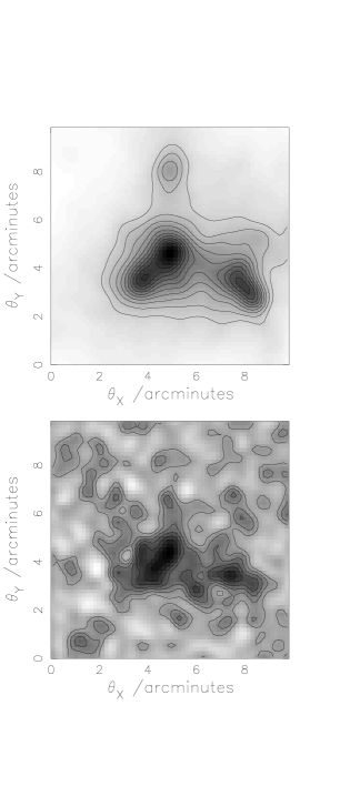
Figure 2: The upper panel shows the projected surface over-density of the N-body cluster which we use as the gravitational lens. The cluster is at a redshift of $z=0.18$ and the surface over-density has been smoothed with a Gaussian of $\theta_{\rm sm}=0.25$ arcminutes. At this redshift 1 arcminute corresponds to approximately $0.24$ Mpc. The lower panel shows the corresponding reconstruction produced from a deep image in 1 arcsec seeing. In each panel the lowest contour corresponds to $\sigma=0$ and the contour spacing is $\Delta\sigma=0.025$. Note that $\sigma$ is the surface density in excess of the mean measured in units of the critical surface density for lensing (see equation 2.6). For the redshift distribution assumed in this case $S_{\rm crit}=3.3\times 10^{15}{\rm M_{\odot}/Mpc^{2}}$

3.3 The Image Plane

Next, we simulate the corresponding image plane. In the weak-lensing regime the bending angle $\vec{\alpha}$ varies continuously and smoothly across the lens plane. Thus, to a good approximation, we can construct the image plane by mapping pixel by pixel the image plane from the source plane. The formula linking the positions of source points and corresponding image points is equation (2.2). This formula allows $\vec{\theta_{s}}$ to be expressed uniquely in terms of $\vec{\theta_{i}}$, but not $\vec{\theta_{i}}$ in terms of $\vec{\theta_{s}}$. For each image pixel we apply this formula and obtain the corresponding point in the source plane. We then assign an intensity to the image pixel by simple bilinear interpolation of the intensities in the nearest four source pixels. This procedure results in a near perfect CCD image of the lensed galaxies. Finally, we add noise to the frame and then convolve it with a Gaussian of width $\theta_{\rm see}$ to simulate sky noise and atmospheric seeing.

3.4 The Inversion

We analyse the image built up in this way using FOCAS. FOCAS (Faint Object Classification and Analysis System) is a software reduction package developed by Jarvis et al. (1981) specifically for measuring properties of faint galaxies. Galaxies have to satisfy certain criteria in order to be “detected”. The user specifies an acceptable level of intensity and a minimum area. After detection FOCAS grows an isophote around each galaxy until it extends as far as the sky noise. The shape of the galaxy is then evaluated within this isophote. The values of intensity-weighted second moments from FOCAS are used to define the ellipticity components $e_{1}$ and $e_{2}$ that feed into equation (2.8) to yield the estimated surface over-density.

The upper panel in Fig. 2 shows the surface over-density distribution of the N-body cluster evolved to redshift $z=0.18$, placed at the corresponding distance and smoothed with a Gaussian of $\theta_{\rm sm}=0.25$ arcminutes. The lower panel shows, at the same resolution, the reconstructed surface over-density map obtained from our simulated CCD image in 1 arcsecond seeing. Although noise features are clearly visible in the reconstruction, the overall morphology is remarkably accurate, reproducing all the major features of the original cluster. We show these plots here as an illustration of the power of the method. In the next section we will investigate the accuracy of the reconstruction in more detail.

4 The reconstruction method in practice

In practice observations of gravitational lensing will not conform to the ideals assumed by the KS reconstruction method. The two most important limitations of real observational data are seeing and noise.

• Seeing

  Seeing is the distortion of images produced by scattering of light as it propagates through the Earth’s atmosphere. Point sources become finite in extent and extended sources like galaxies undergo a corresponding blurring. The resulting effect is to make the galaxies appear more circular. This masks the true elongation of lensed galaxies, making the lens appear less strong and hence reducing the lensing surface over-density recovered by the KS method.

• Noise

  Noise is any spurious signal introduced during the detection process. There are various categories of noise e.g. photon noise, background noise or detector noise. When observing faint galaxies the most important source of noise is the sky background. The shapes of faint galaxies can be grossly distorted by noise. This can confuse the lensing analysis, so very faint galaxies need to be excluded (see Section 4.1).

In addition the KS technique will also break down because of nonlinearity if the surface density of the lens is too high.

• Nonlinearity

  The KS technique is applicable only to weak lensing situations, when second order shear terms are negligibly small i.e. the bending angle varies only slowly, $\partial\vec{\beta}/\partial\vec{\theta}\ll 1$. If the cluster surface over-density is large and varies rapidly this assumption is no longer valid and strong lensing techniques must be employed.

Figure 3: The ratio, $f$, of the true central surface over-density of the lens to the central surface over-density recovered by the KS technique. The upper panel shows the dependence of $f$ on the central surface over-density of the lens for fixed seeing conditions of $\theta_{\rm see}=1$ arcsecond. The lower panel shows the variation of $f$ with $\theta_{\rm see}$ for $\sigma=0.1$.

We illustrate the effect of seeing and non-linearity in Fig. 3. Here we use a simple spherically symmetric lens with a Gaussian mass profile. We vary both the seeing and the mass of the lens, but in each case we keep the noise added to the image frame at a very low level. The factor, $f$, plotted in both panels of Fig. 3 is the ratio of the true surface over-density, $\sigma$, at the centre of the lens, to the corresponding value, $\hat{\sigma}$, recovered by the KS technique. The upper panel shows $f$ as a function of the central surface over-density of the Gaussian lens, for a fixed seeing of $\theta_{\rm see}=1$ arcsecond. We can see that $f$ is constant up to about $\sigma=0.1$ and then increases with increasing surface over-density, implying that nonlinear effects are becoming important for surface over-densities greater than this value and the weak lensing approximation is beginning to fail. The lower panel shows $f$ as a function of seeing. Here the central surface over-density of the Gaussian is kept fixed at $\sigma=0.1$ which, from the upper panel, is still in the regime where the weak lensing approximation appears valid. We can see that $f$ increases rapidly as the seeing worsens.

It is not easy to correct for the systematic error caused by non-linearity. Thus, if the surface over-density at the centre of massive clusters is to be accurately estimated, alternative methods must be employed which take account of non-linearity (C. Seitz & Schneider 1995a; Kaiser 1995). Note, however, that the systematic error is only of order 25% at the centre of a cluster of central surface over-density $0.3$. (Note also that the reason why $f$ does not tend to unity at low values of $\sigma$, in the upper panel of Fig. 3, is the $1$ arcsecond seeing, not residual non-linearity.) Elsewhere in the cluster the systematic error will be smaller.

The systematic error due to the blurring effect of seeing is potentially much larger. If we were able to tabulate the ratio $f$ for all observing conditions, then this table could be used to find a compensation factor to correct the surface over-density estimates returned by the KS technique. However, this is not practical since the effect of seeing depends not only on the value of $\theta_{\rm see}$, but also on intrinsic properties of the galaxy images used in the reconstruction. For example, the degradation due to seeing increases as the angular size of the galaxy images used decreases. To circumvent this problem we outline a calibration procedure in Section 4.2 which can be used to estimate the required compensation factor, $f$, for any given observational dataset.

4.1 Defining the Galaxy Sample

In our simulations we have assumed that stars and cluster galaxies have been removed from the CCD image. In practice, since cluster galaxies are mostly E/S0’s and are all at approximately the same redshift, they have very similar colours and, provided two colour information is available, they are relatively easy to identify. On a colour-magnitude diagram of all objects within the frame, the cluster galaxies will fall on a (nearly) horizontal line (see e.g. Smail 1993) and can be excluded from any subsequent lensing analysis.

Figure 4: The probability that galaxies in any given half-magnitude subsample are drawn from the same distribution of ellipticities as that of the 23.75 to 24.25 subsample. The probabilities are calculated by means of a Kolmogorov-Smirnoff comparison test. Populations fainter than m=25.5 are inconsistent with the brighter populations.

Figure 5: The compensation factor, $f$, versus seeing in realistic signal-to-noise conditions. The line shows the values obtained for $e_{\rm cut}=0.5$

The value of the signal-to-noise ratio in our simulations has been chosen to mimic detections of galaxies down to $m_{B}=26.5$. Although all galaxies down to this magnitude limit are detected in the simulated CCD frame, the faint galaxy shapes are badly contaminated by noise. Thus, it is necessary to make a cut at a brighter magnitude in order to exclude these faint galaxies from the analysis. We find that a useful guide to selecting this magnitude cut comes from looking at the ellipticity distribution of the galaxy images as a function of apparent magnitude. It is to be expected that the intrinsic distribution of $e=\sqrt{e_{1}^{2}+e_{2}^{2}}$ will be a slowly varying function of apparent magnitude. It is, in fact, assumed to be constant in our simulations. Thus, a sudden change in the shape of this distribution at faint magnitudes can most likely be attributed to the onset of noise in the image corrupting the shapes of the faint galaxies. As a quantitative comparison, we divide the data into half magnitude bins and compare the ellipticity distribution in each bin in turn with a representative bright sample using the Kolmogorov-Smirnoff comparison test. As can be seen from Fig. 4, the probability that the two distributions are drawn from the same population plummets to virtually zero at magnitudes fainter than m=25.5. We have found this transition to be a good indication of where to place the magnitude cut used to define the sample of galaxy images to be fed through the KS reconstruction technique. The appropriate value of the cut will depend, of course, on the specific observational set-up.

4.2 Calibration of mass estimator

In this section we describe how to calibrate a CCD frame for use in the KS reconstruction method. Specifically, we show how to compute a compensation factor, $f$, that corrects for the bias in the surface over-density estimates returned by the KS method. Briefly, the procedure involves shearing the galaxy images by a known amount, adding seeing and measuring the resultant shear. The compensation factor, $f$, is then the ratio of the input shear to the measured shear.

If one takes the image frame, multiplies the x-coordinate of each pixel by a factor $1+\epsilon$, and rebins, then all the galaxy images will be sheared in the x-direction. If $\epsilon$ is small and the initial distribution of ellipticities is not too broad then it is easy to show from the definitions (2.9) and (2.10) that the ellipticity component $e_{2}$ of each galaxy is unchanged while the $e_{1}$ component is on average increased by $\epsilon$. If the galaxy images are then blurred by seeing one will find that the measured change in the shear will be somewhat less than $\epsilon$. Since, according to equation (2.8), the surface over-density at any given point is proportional to the measured ellipticities, the ratio of $\epsilon$ to the mean change in $e_{1}$, $\left<\Delta e_{1}\right>$, is in fact the factor $f$ required to correct the surface over-densities, i.e. ,

$$f\equiv\frac{\sigma}{\hat{\sigma}}=\frac{\epsilon}{\left<\Delta e_{1}\right>}$$ (4.20)

This procedure is complicated by two factors. First, the value of $f$ depends on the sizes of the galaxy images (A given value of seeing will produce a much greater circularising effect on small galaxies than on large galaxies). Hence one would underestimate f if the shearing process were applied directly to the enlarged blurred observed images. Second, the initial distribution of $e_{1}$ can be quite broad with some galaxies having values of $e_{1}$ approaching unity prior to addition of any further shear. Since $e_{1}$ is constrained to be less than unity, these high values of $e_{1}$ cannot be increased further. It is therefore necessary both to deconvolve the image prior to applying the shear and to limit the analysis to galaxies whose original ellipticity is less than some value, $e_{\rm cut}$.

In summary, our calibration procedure consists of the following steps:

1. Deconvolve the CCD image using the Point Spread Function measured from one or more stars on the frame. Note that since no analysis is to be made using the deconvolved images, it is not necessary to use sophisticated noise suppressing deconvolution algorithms. Neither is it required to model the PSF in great detail. A Gaussian fitted to the measured PSF is probably adequate.

2. Stretch the galaxy images along the x-axis by a known factor, $1+\epsilon$, and rebin. A value of $\epsilon\approx 0.1$ is appropriate as this is typical of the values produced by weak lensing.

3. Reconvolve the stretched image with the same PSF.

4. Run reduction software on both the original image and this new stretched image and compute the ellipticity components $e_{1}$ and $e_{2}$ for each galaxy.

5. Select the galaxies with measured values of $e<e_{\rm cut}$ in the original frame and, for these, compute the mean change in $e_{1}$, $\langle\Delta e_{1}\rangle$, between the original and stretched frames. Define the compensation factor $f=\epsilon/\langle\Delta e_{1}\rangle$.

6. Estimate the lens surface over-density using the KS method, equation (2.8), with the galaxies selected using the same cut in $e$ as above. Finally, multiply the resulting surface over-densities, $\hat{\sigma}$, by the factor $f$ to yield corrected estimates.

Fig. 5 shows estimates of $f$ obtained by this procedure from simulated CCD frames constructed with realistic signal-to-noise ratios and galaxy populations. Each point is the average obtained from 10 simulated CCD images. The curve shows the compensation factor $f$ for the choice $e_{\rm cut}=0.5$. As expected, we see that $f$ increases rapidly as seeing worsens and that even for good seeing conditions it is significantly different from unity. We use values of $f$ calculated in this way in the next section and show that they give remarkably good estimates of the true surface over-density.

5 Examples and Discussion of Results

We now examine a series of test cases where we explore the success and reliability of the calibrated reconstruction technique for a range of observational conditions and sample selections.

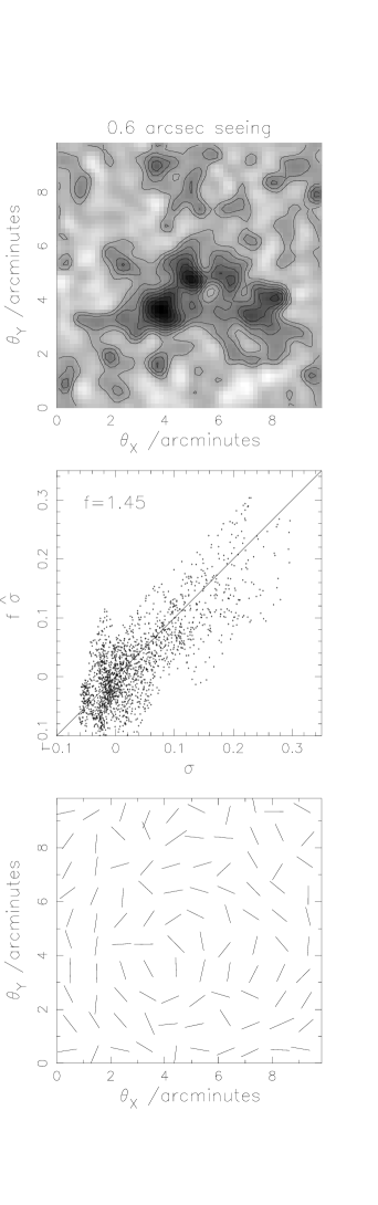
Figure 6: For simulated observations taken in conditions of $\theta_{\rm see}=0.6$ arcseconds seeing the panels show the reconstructed map of the lens surface over-density, a scatter plot of the compensated estimated versus true surface over-density and the estimated shear pattern across the face of the lens, respectively. The value of the compensation factor, $f$, estimated from this data is also shown on the middle panel. The details of the assumed background galaxy properties are detailed in Section 3.1. A magnitude cut, $m_{\rm cut}=25.5$, suggested by the Kolmogorov-Smirnoff test of Section 4.1, and an ellipticity cut of $e_{\rm cut}=0.5$ were used to define the galaxy sample that was analysed.

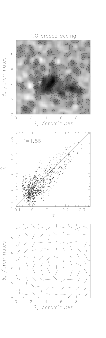
Figure 7: As Fig. 6 but for seeing of $\theta_{\rm see}=1.0$ arcseconds.

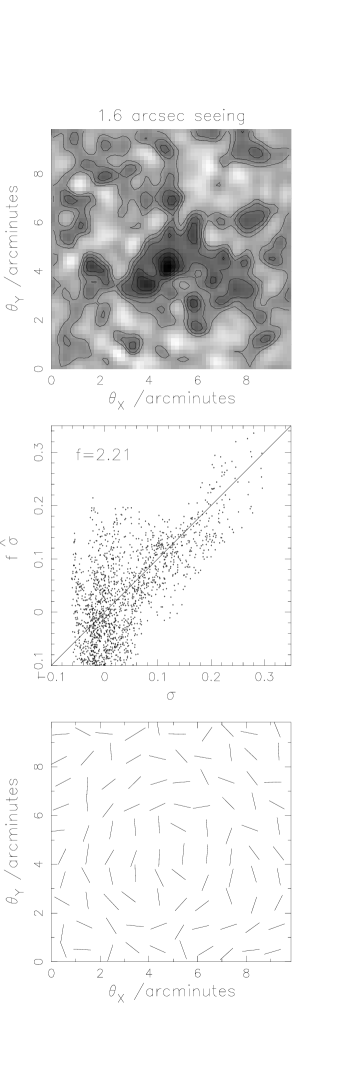
Figure 8: As Figs. 6 and 7, but for seeing of $\theta_{\rm see}=1.6$ arcseconds.

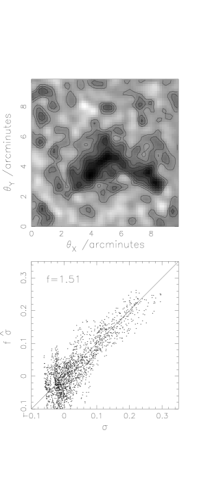
Figure 9: The reconstructed surface over-density map and scatter plot for $\theta_{\rm see}=1.0$ arcseconds (as in Fig. 7), but for galaxies with scale lengths 20% larger than assumed in Fig. 7.

Figure 10: As Fig. 7, but for a narrower distribution of intrinsic ellipticities for the background galaxies. The mean of $b/a$ is now 0.79 compared with 0.71 in Fig 7.

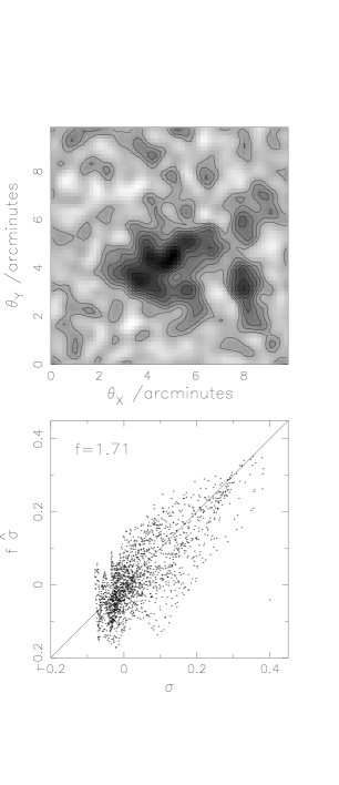
Figure 11: As Fig. 7, but with the background galaxies all at redshift $z=2$.

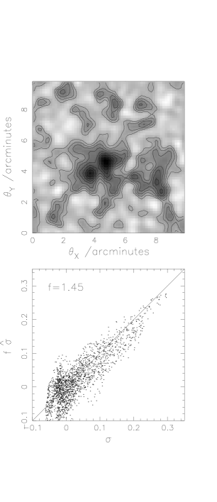
Figure 12: As Fig. 7, but for a deeper CCD frame in which galaxies down to $m_{\rm cut}=26.5$ are retained.

5.1 The Effect of Seeing

Figures 6,7 and 8 show the results of the calibrated reconstruction technique for three different values of the seeing, $\theta_{\rm see}=0.6$, $1.0$ and $1.6$ arcseconds. The upper panel in each figure shows the reconstruction of the cluster surface over-density map. This should be compared to the true lens surface over-density displayed in Fig. 2. The central panel is a scatter plot of the compensated estimated surface over-density versus the true surface over-density measured on a $62\times 62$ grid covering the region shown in the upper panel. The compensation factor $f$ estimated as described in Section 4.2 is shown in the upper left of the panel. The lower panel depicts the mean shear of the galaxies in $10\times 10$ bins, again covering the same area as the map in the upper panel. The length of each line is proportional to the mean ellipticity, $e=\sqrt{\left<e_{1}\right>^{2}+\left<e_{2}\right>^{2}}$, in each cell and the orientations of the lines indicate the direction of the shear.

The first point of note is that the complex morphology of the cluster mass distribution is recovered quite well in all three cases, with only a gradual degradation of the reconstruction as the seeing becomes progressively worse. Second, the value of the compensation factor, $f$, is a strong function of the seeing, varying from $f=1.45$ for $\theta_{\rm see}=0.6$ to $f=2.21$ for $\theta_{\rm see}=1.6$. In spite of this, the compensated surface over-density estimates, $f\hat{\sigma}$, are in good agreement with the true values, $\sigma$, i.e. the points in the central panels all scatter around the line $f\hat{\sigma}=\sigma$, with no significant bias. Finally, we note that equation (2.15) appears to be a good approximation to the variance in the surface over-density estimator; from 9 simulations in 1 arcsec seeing we find a scatter in $\hat{\sigma}$ of 0.052 which compares well with the theoretical value of 0.045.

5.2 Variations in the Properties of the Background Galaxies

In our simulations so far we have assumed specific distributions of the sizes, shapes and redshifts of the background galaxies. These are realistic examples but it is nevertheless important to investigate how our results change when they are varied. In Figs. 9 to 12 we explore the effect on the reconstructed surface over-density maps and scatter plots of varying each of these distributions in turn. In all cases we employ 1 arcsecond seeing and therefore compare our results to Fig. 7. The factors $f$ are now calculated from a single frame rather than from the mean of ten frames as before, so they will be somewhat less reliable.

In Fig. 9 we experiment with the sizes of the galaxies by assuming they are 20 percent larger than before. In this case we might expect the scatter in $f\hat{\sigma}$ to remain unchanged, but $f$ to be reduced since the ratio of galaxy size to seeing is increased. Indeed, the scatter in Fig. 9 is similar to that in Fig. 7 and the value of f is reduced. The scatter does not change because the ellipticity distribution and the noise, the major contributors to the uncertainty, are unchanged.

In Fig. 10 we explore the effect of varying the distribution of intrinsic galaxy ellipticities. We bias the distribution slightly towards less elliptical galaxies, so that the mean axial ratio is $b/a=0.79$ rather than $b/a=0.71$ as before. We see from the figures that the resulting effect is to reduce the scatter in accordance with equation (2.15). Although the value of f shown here is slightly diminished, the mean value of f from 5 frames is little changed.

In Fig. 11 we use a deeper distribution of galaxy redshifts, namely placing all the galaxies at $z=2$. This change reduces the value of $S_{\rm crit}$ (see equation 2.6) and increases the values of $\sigma$ and $\hat{\sigma}$ proportionally at all grid points. This is the reason for the change of scale on the axes compared with the previous figures. Since the values of $\sigma$ and $\hat{\sigma}$ increase in the same ratio, the mean value of $f$ is unchanged.

In our final plot, Fig. 12, we increase the signal-to-noise ratio so that galaxies can now be detected one magnitude fainter than before. The higher galaxy number density greatly reduces the scatter in $f\hat{\sigma}$, as expected from equation (2.15). The compensation factor is also reduced somewhat because the galaxy shapes are now less distorted by noise than before.

6 Conclusions

We have performed a series of controlled experiments to assess the reliability of the technique proposed by Kaiser & Squires (1993) to reconstruct the surface mass over-density of galaxy clusters from observations of weak gravitational lensing. In particular, we have tested the KS method on a realistic cluster mass distribution, typical of those expected in an $\Omega=1$ universe. By simulating data from standard observing conditions, we have investigated the effects of seeing and signal-to-noise on the reconstructed dark matter maps and we have explored how the results vary with different assumptions for the distributions of intrinsic galaxy shapes and redshifts. Our main conclusions are as follows:

1. With a careful analysis of data obtained in standard observing conditions, the KS method provides a remarkably faithful reconstruction of the morphology of a complex cluster, reproducing the richness of structure expected in an $\Omega=1$ universe.

2. Our simulations show that the weak lensing assumption on which the KS technique is based begins to break down when the mass surface over-density exceeds 10% of the critical surface density. However, even when it equals 30% of the critical value, the KS method underestimates the surface over-density by only $\sim 25$%. The noise in the reconstructed maps agrees well with a simple estimate (equation 2.15) of the uncertainties due to Poisson noise and to the scatter in the intrinsic ellipticities of the lensed background galaxies.

3. The simple calibration procedure for CCD images which we have designed and tested, efficiently corrects for the effects of atmospheric seeing on the reconstructed mass surface over-density maps. This procedure is straightforward to apply to CCD data and yields a multiplicative “compensation factor”, $f$, which allows the true surface over-density in each pixel (in units of the critical density) to be recovered from the reconstructed map. The absolute value of the lens mass cannot be derived by this method unless the critical density, which depends on the redshift distribution of the lensed galaxies, is known. However, the dependence on redshift is fairly weak (see e.g. Fig 5 of Blandford & Kochanek, 1987).

4. Our method for calculating the compensation factor is quite robust. The value of $f$ is primarily determined by the seeing, but the depth of the CCD image and the intrinsic properties of the lensed galaxies also affect it. Useful results can be obtained even with data acquired in seeing as large as 1.6 arcseconds, although the technique clearly works best with sub-arcsecond seeing. Our simulations indicate that it should work well when applied to data obtained in a wide range of observing conditions, allowing useful mass reconstructions to be made even when the correction factor is as large as $f=2$.

References

- [1994] Arnaud M., 1994, in Seitter W. C., ed, Cosmological Aspects of X-ray Clusters of Galaxies, Kluwer Academic Publishers, p.197
- [Bartelmann & Weiss 1994] Bartelmann M., Weiss A., 1994, A&A, 287, 1
- [1994] Bartelmann M., Narayan R., 1994, in Holt S. S. and Bennet C. L., eds, Proc. 5th Annual Maryland conference, Dark Matter in the Universe, AIP Press, p307
- [Bartelmann & Narayan 1995] Bartelmann M., Narayan R., 1995, ApJ, 451, 60
- [Bartelmann 1995] Bartelmann M., 1995, A&A, 299, 11
- [Blandford & Kochanek1987] Blandford R., Kochanek C., in Proc. 13th Jerusalem Winter School, Dark Matter in the Universe
- [Bonnet et al. 1993] Bonnet H., Mellier Y., Fort B., 1994, ApJ, 427, L83
- [Brainerd et al. 1995] Brainerd T. G., Blandford R. D., Smail I., 1995, ApJ, in press
- [Broadhurst et al. 1995] Broadhurst T. G., Taylor A. N., Peacock J. A., 1995, ApJ, 438, 49
- [Broadhurst 1994] Broadhurst T. G., 1994, in Holt S. S. and Bennet C. L., eds, Proc. 5th Annual Maryland conference, Dark Matter in the Universe, AIP Press, p320
- [Carlberg et al. 1994] Carlberg R. G., Yee H. K. C., Ellingson E., 1994, ApJ, 437, 63
- [Cole et al. 1994] Cole S., Aragon-Salamanca A., Frenk C. S., Navarro J. F., Zepf S. E., 1994, MNRAS, 271, 781
- [Davis et al. 1994] Davis M., Efstathiou G., Frenk C. S., White S. D. M., 1985, ApJ, 292, 371
- [Evrard et al. 1994] Evrard A. E., Mohr J. J., Fabricant D. G., Geller M. J., 1994, ApJ, 419, L9
- [Fabian 1988] Fabian A. C., 1988, in ed., R. Pallaviani, Hot Thin Plasmas in Astrophysics, Kluwer Academic Publishers, p.293
- [Fahlman et al. 1994] Fahlman G., Kaiser N., Squires G., Woods D., 1994, ApJ, 437, 56
- [Fort & Mellier 1994] Fort B., Mellier Y., 1994, A&AR, 5, 239
- [Frenk et al. 1990] Frenk C. S., White S. D. M., Efstathiou G., Davis M., 1990, ApJ, 351, 10
- [Frenk et al. 1995] Frenk C. S., Evrard A. E., White S. D. M., Summers F. J., 1995, ApJ, in press
- [Hughes1989] Hughes, J.P., 1989, ApJ, 337, 21
- [Jarvis & Tyson 1981] Jarvis J. F., Tyson J. A., 1981, AJ, 96, 476
- [Kaiser 1992] Kaiser N. ,1992, ApJ, 388, 272
- [Kaiser & Squires 1993] Kaiser N., Squires G., 1993, ApJ, 404, 441
- [Kaiser et al. 1994a] Kaiser N., Squires G., Fahlman G., Woods D., 1994a, in Proc. Meribel conference, Clusters of Galaxies
- [Kaiser et al. 1994b] Kaiser N., Squires G., Fahlman G., Woods D., Broadhurst T. G., 1994b, in Maddox S. J. and Aragon-Salamanca A., eds, Proc. Herstmonceux conference, Wide Field Spectroscopy and The Distant Universe, Kluwer Academic Publishers, p246
- [Kaiser 1995] Kaiser N., 1995, ApJ, 439, L1
- [Kaiser et al. 1995] Kaiser N., Squires G., Broadhurst T. G., 1995, ApJ, 449, 460
- [Kneib 1993] Kneib J. P., 1993, University of Toulouse Ph.D. thesis
- [Kochanek 1990] Kochanek C. S., 1990, MNRAS, 247, 135
- [Lacey & Cole 1993] Lacey C., Cole S., 1993, MNRAS, 262, 627
- [Lynds & Petrosian 1986] Lynds R., Petrosian V., 1986, Bull. Am. Astron. Soc., 18, 1014
- [Mellier et al. 1993] Mellier Y., Fort B., Kneib J. P., 1993, ApJ, 407, 33
- [Metcalfe et al. 1995] Metcalfe N., Shanks T., Fong R., Roche, N., 1995, MNRAS, in press
- [Miralda-Escude 1991] Miralda-Escude J., 1991, ApJ, 370, 1
- [Mohr1995] Mohr J. J., Evrard A. E., Fabricant D. G., Geller M. J., 1995, ApJ, 447, 8
- [Press et al. ] Press W. H., Flanery B. P., Teukolsky B. P., Vetterling W. T., Numerical Recipes, Cambridge University Press
- [Schneider et al. 1992] Schneider P., Ehlers J., Falco E. E., 1992, Gravitational Lenses, Heidelberg:Springer
- [Schneider & Seitz 1995] Schneider P., Seitz C., 1995, A&A, 294, 411
- [Seitz & Schneider 1995a] Seitz C., Schneider P., 1995a, A&A, 297, 287
- [Schneider 1995] Schneider P., 1995, A&A, 1995, in press
- [Seitz & Schneider 1995b] Seitz S., Schneider P., 1995b, A&A, in press
- [Smail et al. 1994] Smail I., Ellis R., Fitchett M., Edge A., 1994, MNRAS, 273, 277
- [Smail 1993] Smail I., 1993, University of Durham Ph.D. thesis
- [Soucail 1987] Soucail G., Fort B., Mellier Y., Picat J. P., 1987, A&A, 172, L14
- [Squires 1994] Squires G., 1994, private communication
- [Squires 1995] Squires G., Kaiser N., Babul A., Fahlman G., Woods D., Neumann D. M., Bohringer H., 1995, preprint
- [Tyson et al. 1990] Tyson J. A., Valdes F., Wenk R., 1990, ApJ, 349, L1
- [Tyson & Fischer 1995] Tyson J. A., Fischer P., 1995, ApJL, 446, L55
- [Tyson 1994] Tyson J. A., 1994, in Schaeffer R. et al. , eds, Proc. Les Houches Summer School, Cosmology and Large Scale Structure, Elsevier Scientific Publishers
- [Valdes et al. 1983] Valdes F., Tyson J. A., Jarvis J. F., 1983, ApJ, 271, 431
- [Wilson et al. 1994] Wilson G., Cole S., Frenk C. S., 1994, in Holt S. S. and Bennet C. L., eds, Proc. 5th Annual Maryland conference, Dark Matter in the Universe, AIP Press, p351
- [Wilson et al. 1995] Wilson G., Smail I., Ellis R., Frenk C. S., Couch W. J., 1995, in preparation