Redshift Surveys and Large–Scale Structure

Abstract

I review the present status of the mapping of the large–scale structure of the Universe through wide–angle redshift surveys. In the first part of the paper, I discuss the current state of the art, describing in some detail the recently completed ESO Slice Project. In the second, I recall some of the basic motivations for performing larger surveys. Then, in the final section, I present in detail the three large redshift survey projects that in the years from now to the end of the Century are expected to satisfy this demand.

Osservatorio Astronomico di Brera, Via Bianchi 46, I–22055, Merate (LC), Italy

1. Introduction

In preparring my contribution for this meeting, I thought it was a good moment to stop and to try and summarize the presently fervent activity in mapping the large–scale distribution of luminous matter, with a special look at the large redshift projects which are currently in their early phases. In fact, during these last twenty years since when Chincarini & Rood (1976) recognized the “segregation of redshifts” in their maps of the surroundings of the Coma cluster (actually the embryo of the following CfA surveys), the industry of redshift measurements has skyrocketed. As a consequence, our knowledge of, at least, the local (cz $<10000$ km s^-1) Universe has greatly improved (see Rood 1988 for a colourful account of the pioneering years; more recent reviews can be found in Giovanelli & Haynes 1991, and Strauss & Willick 1995). Still, all the surveys within this depth show inhomogeneities of comparable size (e.g. the Great Wall in the North Galactic Cap, Geller & Huchra 1989, or the Perseus–Pisces filament in the South, Giovanelli et al. 1986), making it difficult to think of them as statistically representative.

The development of wide–field multi–object (MOS) spectrographs using fibre optic advanced technology represents the key for the further giant step in the mapping of large–scale structure. The first two wide–angle surveys using fibre spectrographs, the ESO Slice Project and the Las Campanas Redshift Survey, have been recently completed, pushing the depth of the samples to six times that of CfA2 (section 2.). However, the need for larger, more three-dimensional maps is still strong, as I shall briefly outline in section 3. There are three large mapping projects which are expected to fill this gap, two using galaxies and one using clusters of galaxies. These, the Sloan Digital Sky Survey, the 2dF survey and the ESO Key–Programme survey of ROSAT clusters will be discussed in some detail in the last section.

2. Cosmic Maps: the Present Picture

In terms of redshift surveys we can now talk of the “local” Universe as that mapped by the CfA2 and SSRS redshift surveys, to a depth of $\sim 100\;{\rm h}^{-1}\;{\rm Mpc}$. I will not discuss here the many important results obtained from this combined data set (for which details can be found, e.g., in Park et al. 1994), but prefer to concentrate on the results from the first large multiplexed surveys. I will also not discuss here all the series of redshift surveys based on the IRAS catalogue (treated exhaustively by Rowan–Robinson in this same volume), and sparse surveys like the APM/Stromlo (Loveday et al. 1992).

By multiplexing, one means one of the major technological advances in the field of astronomical spectroscopy, i.e. the development of Multiple–Object spectrographs. These give simply the possibility of coupling more than one slit or aperture in the focal plane of the telescope to the spectrograph, collecting many spectra at once. This is performed either through redirection of the light beam by means of optical fibres, or through slitlets carved out of a metal mask placed in the focal plane. While the latter instruments (e.g. EFOSC at the ESO 3.6 m telescope) have their field of view limited by the size of the detector, typically a few arcminutes, fibre spectrographs can exploit the whole corrected field of the telescope, with diameters of the order of 1 degree (see e.g. the review by Hill 1988).

The impact of multiplexing on large–scale redshift work is readily understood by considering as an example the case of the ESO Optopus system, with 50 fibres over a 30 arcmin field at the Cassegrain focus of the ESO 3.6 m telescope. The density of fibres on the sky for this instrument is then $\sim 250$ deg^-2. If we consider the number counts law for an euclidean geometry,

$$N(<m)=N_{\circ}\;10^{0.6m}$$ (1)

one can then ask for which value of $m$ the mean number counts will match the density of fibres, and find that (e.g. in the IIIaJ blue band) this happens for $m_{b_{J}}\sim 19-19.5$. The simple introduction of a similar instrument, therefore, immediately pushes the potentially optimal magnitude limit to four magnitudes deeper than the CfA2.

2.1. The ESO Slice Project

The ESO Slice Project (ESP) is a first example of a large–scale, wide–angle galaxy redshift survey performed by mapping the sky through a fibre spectrograph, and actually the very first of such surveys using one of the ESO telescopes. The ESP started in 1991, after a number of unsuccesfull attempts and in a somewhat reduced form with respect to the original idea. It covers a $32^{\circ}\times 1^{\circ}$ strip at constant declination, (with a $5^{\circ}$ gap), centered at $\delta-40^{\circ}$, using the Optopus fibre spectrograph at the 3.6 m ESO telescope. The strip is mapped with a regular grid of Optopus fields, observing all the galaxies with $b_{J}\leq 19.4$ in the Edinburgh–Durham Southern Galaxy Catalogue (EDSGC, Heydon–Dumbleton et al. 1989). This magnitude limit, which optimizes the fibre coupler, results in an effective depth of $\sim 600\;{\rm h}^{-1}\;{\rm Mpc}$. The optical fibres cover 2.4 arcsec on the sky, and are manually plugged into a pre–drilled aluminum plate. The data are now fully reduced, and the final redshift catalogue contains 3348 galaxies. The overall redshift yield of the survey has been larger than 80%. More details can be found in Zucca et al. (1996).

Fig. 1 shows a wedge diagram of the whole ESP data. The first qualitative impression when comparing this plot to, e.g., the CfA survey slices, is that there does not seem to be any structure with dimensions comparable to the survey size. Are we finally approaching a fair sample of the Universe?

Figure 1.: The ESO Slice Project data, for $cz\leq 60000\;km\;s^{-1}$. The slice is $1^{\circ}$ thick, comprised between -39^∘ 45^′ and -40^∘ 45^′ in declination.

A rather large fraction of galaxies in the survey ($\sim 50\%$) show emission lines in their spectra ([OII] $\lambda 3727$, $H\beta\;\lambda 4861$, [OIII] $\lambda 4959$ and $\lambda 5007$). These objects could be either spiral galaxies, where lines originate mostly from HII regions in the disk, or starburst galaxies. Their distribution is different from that of galaxies without emission lines, a fact that could either be a manifestation of the known morphology–density relation, or indicate that starburst phenomena occur preferentially in low density environment, or both.

Most of the effort in the analysis of the new ESP data has been devoted so far to the study of the luminosity function (LF). This has involved a careful study of the K–correction. In particular, since galaxy morphology, a necessary ingredient to the K–correction, is not discernible for most of the galaxies in the survey, a statistical approach was adopted as discussed in Zucca et al. (1996). The Schechter function is a good fit to the data for $M_{b_{J}}<-16$, as shown in fig. 2a. At fainter luminosities (down to $-12$), a statistically significant raise above the Schechter form is detected (see Vettolani et al. 1996). The best estimate of the Schechter shape parameters, based on 3311 galaxies and using the maximum likelihood method of Sandage et al. (1979) (with arbitrary normalization), gives $\alpha=-1.23$ and $M^{*}_{b_{J}}=-19.61$. An interesting result is obtained when the LF is estimated separately for galaxies with and without emission lines, as shown in fig. 2b. The difference in the parameters is very significant, with the population of line–emitting objects rising steeply towards fainter magnitudes.

Figure 2.: a) The ESP luminosity function for $M_{b_{J}}<-16$, estimated using a modified version of the non–parametric C–method (Lynden–Bell 1971). The inset shows the maximum–likelihood 68% and 95% confidence ellipses on $\alpha$ and M^∗. b) Normalized Schechter fits to the luminosity functions for ESP galaxies with (solid line) and without (dotted line) emission–lines. Note the very significant separation in parameter space of the two data sets. (From Vettolani et al. 1996).

2.2. The Las Campanas Redshift Survey

The other large multiplexed redshift survey recently completed is the Las Campanas Redshift Survey (LCRS). It has been performed by the so–called KOSS collaboration (see e.g. Shectman 1995), using a 112–fibre spectrograph with a 1.5^∘ diameter field at the Cassegrain focus of the Du Pont 2.5 m telescope. This is at present the largest survey available, with nearly 25000 redshifts. Similar in depth to the ESP, but selected in the red band from CCD exposures, it covers a larger area – about 700 deg² – distributed among 6 strips. There is not enough space here to detail further on this project. The reader is referred to the contribution by Landy, in this same volume, and to references therein. In particular, see Tucker (1994) for a comprehensive discussion of the sample construction, and Lin (1995) for an account of various statistical analyses.

3. Quantitative Needs for Larger Surveys

I have deliberately selected two scientific issues which contain in my view the main motivations for larger redshift surveys. I will discuss them here in a very schematic way.

3.1. Correlation Function and Power Spectrum

The correlation function $\xi(r)$ and its Fourier transform, the power spectrum $P(k)$ are some of the simplest, but most important clustering statistics (e.g. Peebles 1980). Estimates of $P(k)$ from present redshift surveys (e.g. Park et al. 1994), or large angular catalogues like the APM survey (Baugh & Efstathiou 1993) are limited to wavelengths $\sim 100\;{\rm h}^{-1}\;{\rm Mpc}$. Even at smaller scales the effective slope of the power spectrum [or the shape of $\xi(r)$], is poorly constrained, with strong variations from sample to sample (see e.g. Branchini et al. 1994 and references therein). On the other hand, the constraints on the matter power spectrum from microwave background anisotropy measurements as those provided by COBE (Smoot et al. 1992), are on scales of $\sim 1000\;{\rm h}^{-1}\;{\rm Mpc}$. Larger surveys are therefore necessary in order to: a) establish the slope of $P(k)$ at $\lambda\sim 10-100\;{\rm h}^{-1}\;{\rm Mpc}$; b) determine the scale where $P(k)$ turns over [or equivalently $\xi(r)$ goes negative]; extend the estimates of $P(k)$ from large–scale clustering into a regime overlapping with the CMB data.

The LCRS provides interesting hints on $P(k)$ out to wavelengths of $\sim 300\;{\rm h}^{-1}\;{\rm Mpc}$ (Lin 1995), but it is still limited in the accuracy at such wavelengths due to the survey geometry. The ESP, being a single slice, is going to have similar problems in this respect, obviously worsened by the lower sampling. Clearly, 3D surveys with typical depth similar to ESP and LCRS, but covering wider sky areas are the key for these issues.

3.2. Connection to Dynamics: Redshift Space Distortions

The anisotropy introduced by peculiar velocities on the observed maps of the galaxy distribution is reflected by distortions in the correlation function and power spectrum computed in redshift space. These distortions can be modelled and contain a wealth of information about the large–scale density field. Distortions at small scales are intimately related to the amount of small–scale power in the power spectrum, i.e. the relative “temperature” of galaxy pairs. A low value ($\sim 340$ km s^-1) for the pairwise velocity dispersion at $1\;{\rm h}^{-1}\;{\rm Mpc}$ $\sigma_{12}(1)$ has been assumed for many years, on the basis of the result from the CfA1 survey (Davis & Peebles 1983). While IRAS galaxies seemed to confirm this figure (Fisher et al. 1994), more recently, a tendency towards a value closer to ($\sim 600$ km s^-1) has been found in the analysis of larger optical samples (Guzzo et al. 1995; Marzke et al. 1995; see also Zurek, this volume), but still with large (up to 50%) fluctuations depending on the volume sampled. That from the full LCRS ($\sim 500$ km s^-1, Lin 1995), is probably the first estimate sampling a sufficient volume ($\sim 5\times 10^{6}$ Mpc³) to start seeing convergency of $\sigma_{12}(1)$.

Distortions of $\xi(r)$ and $P(k)$ in the linear regime (i.e. at large separations) work in the opposite sense: they are produced by coherent motions when these are seen parallel to the line of sight and have the effect of amplifying clustering. The amplification is approximately expressed as $\beta\simeq{\Omega^{0.6}/b}$ (Peebles 1980). Here $b$ is the bias factor, the ratio between the rms fluctuations in the galaxies and in the mass. By modelling the distortions produced on $\xi(r)$ or $P(k)$, under the natural hypothesis of a fully isotropic underlying clustering process, it is possible to estimate $\beta$ (e.g. Fisher et al. 1994; Cole et al. 1995). However, this is true only if the survey is geometrically fair, i.e. does not present a dominance of one or a few structures along some preferred directions. This is clearly not the case for $m\leq 15.5$ surveys containing the Great Wall or the Perseus Pisces chain. The LCRS finds $\beta=0.50\pm 0.25$ (Lin 1995). Structures in this and the ESP survey finally seem to be significantly smaller than the sample size. However, the errors on $\beta$ can be improved only with an even larger volume sampled.

4. The Next Step

During the next five years at least three major survey projects covering scales that approach the $\sim 1000\;{\rm h}^{-1}\;{\rm Mpc}$ realm will be completed.

4.1. The Sloan Digital Sky Survey

Undoubtedly, this represents the largest and most comprehensive galaxy survey work ever conceived. It will provide not only direct new results of high scientific impact, but also build a large photometric and spectroscopic data base to be released to the scientific community soon after completion of the survey. The information on the SDSS discussed here come primarily from the paper by Gunn & Weinberg (1995, GW95 hereafter), to which the reader is referred for details, and from discussions with SDSS project members. Further information can be found on the SDSS www page (http://www-sdss.fnal.gov:8000/).

The project is conducted by a large consortium of U.S. Institutions (with the participation of the National Observatory of Japan), which has built a dedicated 2.5 m telescope with a corrected field of $3^{\circ}$ in diameter.at Apache Point, New Mexico. The auxiliary instrumentation includes a battery of 30 $2048^{2}$ CCDs distributed over six columns, which will perform imaging in drift scanning mode. Another 24 smaller service CCDs will take care of astrometric calibration and focusing. The photometric work will be further assisted by an automatic 0.7 m telescope equipped with a CCD camera and the same filter set used in the survey camera. This service instrument will observe a network of standard stars to determine extinction corrections and set accurate zero points for the calibration of both the photometric and possibly (through narrow–band filters) spectrophotometric data.

For the spectroscopy, two double fibre spectrographs with 320 fibres each will be used. Each of them will have a blue and red channel, with independent cameras and gratings on each arm. Interestingly enough, the fibre placing strategy has resorted back to the classic hand–plugging method on pre–drilled plates. With ten fibre harnesses, and a total observing–plus–overhead time per plate of about a hour, all the plugging work of one night can be done during the day. In fact, with two spectrographs available that permit to mount the plugged plate on one while the other is observing, this solution does not compromise the survey efficiency while allowing a significant simplification and reduction of costs.

Figure 3.: A $6^{\circ}$ by $130^{\circ}$ slice extracted from a large N–body simulation of a low–density ($\Omega=0.4$, $\Lambda=0.6$) CDM model performed by Park & Gott (from GW95). The slice is in redshift space and the selection function has been constructed to reproduce that expected for the SDSS. The whole survey will contain about 15 times the number of galaxies plotted here.

The essential features of the survey can be summarized as follows:

• Photometry (S/N=5) in five bands ($u^{\prime}$, $g^{\prime}$, $r^{\prime}$, $i^{\prime}$, $z^{\prime}$), respectively to a depth of 22.3, 23.3, 23.1, 22.3, 20.8 over $10^{4}$ $deg^{2}$ in the whole North Galactic Cap. $200$ deg² in the South Galactic Cap will be also surveyed to about 2 magnitudes deeper in each band.

• This will result in the detection of $\sim 5\times 10^{7}$ galaxies and $\sim 10^{8}$ stars over the $\sim\pi$ steradians of the survey. From the latter set of point–like sources, a subset of $\sim 10^{6}$ colour–selected candidate QSOs will be extracted.

• Medium resolution spectroscopy for the $\sim 10^{6}$ galaxies brighter than $r^{\prime}\sim 18$, the $\sim 10^{5}$ QSOs brighter than $g\prime\sim 19$ and for specific subsets of stars.

• The first test year of the SDSS will possibly be started by the time these proceedings are published. The important feature for the community is that the SDSS consortium is committed to releasing the first two years of data within four years from the start of the survey and to opening a public data archive within two years of its completion, expected within 5 years from the start.

The description of the instrumentation and of the survey strategy clearly shows how the aims of the SDSS are well beyond the pure mapping of the large–scale distribution of galaxies over the chosen volume. For a large fraction of the galaxies, one will have good signal–to–noise photometrically calibrated spectra, with excellent (3900–9100 Å) spectral coverage, in addition to the multi–colour and morphological data from the imaging survey. Fig. 3 gives an idea of how a $6^{\circ}$ slice through the SDSS should look like. It shows a mock galaxy catalogue extracted from a $600\;{\rm h}^{-1}\;{\rm Mpc}$–side simulation by C. Park & R. Gott, containing 54 million particles and started from $\Omega=0.4$, $\Lambda=0.6$ CDM initial conditions (GW95). The reader might find interesting comparing the qualitative features of this slice to the real data (with much shallower sampling), of fig.1.

4.2. The 2dF Project

The 2dF fibre facility at the prime focus of the Anglo–Australian Telescope represents the natural evolution of the UK/Australia leading tradition in fibre optic instrumentation for wide–field spectroscopy. 2dF is an acronym for “2–degree–Field”, which indicates the main feature of this instrument, namely the capability of producing corrected images over a $2^{\circ}$ field of view, to be then fed into a powerful 400–fibre automatic positioner. With respect to previous AAT fibre facilities (FOCAP, AutoFib), this implies a gain of $\sim 9$ in area coverage, while keeping a similar fibre density on the sky ($\sim 130$ deg^-2 vs. $\sim 170$ deg^-2). The obvious consequence is a similar gain in the total telescope time required to survey a given area to the same depth. Further extending the AutoFib concept, the fibres are automatically positioned by a flying positioner and magnetically held onto a metal plate placed at the focal surface. To minimize time losses due to reconfiguration of the fibres, the fibre coupler is doubled, so that one field is configured while the previous one is being observed. The 400 fibres are split into two bundles, which feed two independent spectrographs mounted on the telescope top ring. For further details, see Taylor (1995).

The most obvious application of the 2dF facility is large–scale structure studies. This is what has been succesfully proposed by a UK/Australia team, with what is now known as the “2dF Survey”. The project concentrates on spectroscopy and aims at collecting spectra for 250000 galaxies to around $b_{J}\leq 19.7$ (plus a faint extension of further 10000 objects). Galaxies will be selected from the APM and EDSGC catalogues. The geometry of the survey will be a combination of a large, contiguous volume with randomly placed fields. Two contiguous areas of $75^{\circ}\times 12.5^{\circ}$ and $65^{\circ}\times 7.5^{\circ}$, respectively in the South and North galactic caps will be fully covered with a honeycomb of 2dF fields, yielding a total of $\sim 210000$ galaxies. In addition, 100 randomly–placed fields over the entire southern APM area will provide further $\sim 40000$ redshifts over a very large volume. (It is somewhat amazing to consider that these 40000 spectra will be collected in less than 10 nights). This latter strategy is an interesting feature of the survey, aimed at maximising the large–scale signal in the power spectrum whilst keeping the telescope time within limits acceptable for a general purpose telescope like the AAT. Clearly, the SDSS does not need to resort to such strategical sparse–sampling techniques, since it will fully cover (in the North cap), the same area which is sparsely surveyed by the 100 2dF fields in the South.

See http://msowww.anu.edu.au/$\sim$colless/2dF/ for further information.

4.3. The ESO Redshift Survey of ROSAT Clusters

The third large–scale project which in the next few years will produce a sample exploring scales of the order of $1000\;{\rm h}^{-1}\;{\rm Mpc}$ involves the use of clusters of galaxies as tracers of large–scale structure.

Clusters of galaxies are the largest structures in the Universe to have clearly separated from the Hubble flow, recollapsing to what can be considered to some extent a virialized dynamical configuration. Clusters contain a large quantity of gas at temperatures of 1–10 keV, which emits in the soft X–ray band with typical luminosities around $10^{44}$ erg s^-1 (see e.g. Sarazin 1986; Böhringer 1995). X–ray clusters can therefore be conveniently used as tracers of the large–scale structure of the Universe (see Guzzo et al. 1995, and Böhringer 1995 for a more detailed discussion). A redshift survey of clusters of galaxies based on a an X–ray wide–area imaging survey represents an optimal complement to optically selected galaxy redshift projects. A large 3D catalogue of X–ray galaxy clusters would provide a way to estimate the power spectrum not only through the usual clustering analysis, but also (at smaller mass scales), from the luminosity and temperature distribution functions. The best available X–ray imaging survey from which starting to construct such a sample is certainly the ROSAT All Sky Survey (RASS), performed at the end of 1990 by the ROSAT satellite in the 0.1–2.4 keV energy band (Trümper 1992; Voges 1992; Böhringer 1994). The first survey processing by the so–called Standard Analysis Software System (SASS), yielded a database of some 50000 sources, with 4000–5000 of these expected to be clusters of galaxies. Early after completion of SASS, cluster follow–ups started on specific areas like e.g. the South Galactic Pole region (Romer et al. 1994; see Böhringer 1994 for a review).

Here I would like to describe in detail the ESO redshift survey of ROSAT clusters of galaxies, an ESO Key–Programme started in 1992 by a large European team with the aim of measuring the mean redshift of all southern clusters with $|b|\geq 20^{\circ}$ and flux larger than 1.6–2$\times 10^{-12}$ erg s^-1 cm^-2 (Guzzo et al. 1995). The total sample includes $\sim 700$ clusters, and I shall refer to it as the KP hereafter.

Cluster Identification

Given the 50000 sources detected by SASS, the first step for constructing a complete sample is to identify which of these are in fact clusters. Clearly, even if it would be highly desirable, direct CCD imaging of all SASS sources is presently not feasible, a part from some specific regions where full indentification is carried out by a specific project at ESO. Given the size of the KP, an automatic approach had to be applied. Even before starting this identification process, however, one has to worry on whether the source detection algorithm of SASS has actually detected all the sources associated with clusters of galaxies. In fact, it turns out that nearby, very extended clusters are in fact missed by SASS. This seems to happen only for $z<0.015$, as discussed in the following. Once the SASS source list is taken for granted, the main identification is then performed by cross–correlating the position of the X–ray sources with that of all optical galaxies with $b_{j}\leq 20.5$ in the southern sky. Galaxy positions, magnitudes and shape parameters are taken from a large reference catalogue, constructed in Edinburgh with the COSMOS and SUPERCOSMOS machines from the whole southern sky ESO/SRC J survey plates, and handled through a collaboration among MPE, ROE–Edinburgh and NRL–Washington. A source is identified as a candidate cluster if it corresponds to a local excess in the counts with respect to a certain threshold. Given the magnitude limit of the galaxy catalogue, the resulting sample of clusters has a cutoff at a redshift around $z\sim 0.25-0.3$. The selection function of the KP, given its flux limit, peaks at redshifts between 0.1 and 0.2, so that the redshift cutoff has a limited effect on the resulting sample. We also complement the resulting candidate list with the sources classified as extended in the SASS, but not picked up by the galaxy excess method. Although the SASS extension parameter has proven not to be a fully reliable estimator (De Grandi, 1996), this further selection recovers a few clusters missed by the galaxy excess method for a number of reasons (e.g. crowding of galaxies). At the same time, it picks up some intrinsically very large and luminous objects at $z>0.3$, of particular interests even as single objects.

Flux Estimation: a Pilot High–Quality Subsample

Once all the SASS sources candidate for being associated to a cluster have been identified, a flux–limited sample of clusters can be constructed. However, as it was recognized early, SASS has the tendency to underestimate the count rates for extended sources by about a factor of 2 in the mean, (Ebeling, 1993). A specific effort to understand the survey data and re–estimate the X–ray fluxes was then required for assuring the eventual selection of a complete, truly flux–limited X–ray sample for the KP. Part of this has been done by Sabrina De Grandi for her PhD thesis work (1996). This pilot study concentrates on the South Galactic Cap region, and to a final flux limit of $3\times 10^{-12}$ erg s^-1 cm^-2, i.e. about twice as high as that of the final KP sample. The method developed has a number of advantages: 1) it uses the correct RASS point spread function (PSF), which has broader wings with respect to the simple Gaussian adopted, e.g., in the SASS; 2) it allows the derivation of a physical extension of the cluster candidates (the core radius), modelling the profile through a truncated King formula with $\beta=2/3$, convolved with the PSF; 3) through the same profile, it computes the total counts recovering the missing flux from the source wings. The estimator is robust, being based on the ratio of two integrals of the King profile (and for this reason called the Steepness Ratio method), and has been tested extensively on sets of well–known sources. Fig.4 (left panel) plots the new estimate of the count rates against the corresponding SASS count rates, performed on the set of candidate KP clusters in the pilot area. Note the trend, with the more extended sources being those more underestimated by SASS. Also, due to the dispersion of the relation, any initial cut in the SASS count rates is reflected by a much brighter cut in the “true” counts, if a complete sample has to be obtained. The same kind of plot done without any initial cut, shows that with an initial SASS threshold at 0.055 cts s^-1, the selection at corrected count rates $>$ 0.25 cts s^-1 gives a completeness $\geq$ 96%. The 4% of missed objects can be shown to correspond to very extended sources with angular core radius $\theta_{c}\geq$ 9.7^′. For $r_{c}=0.125\;{\rm h}^{-1}\;{\rm Mpc}$, this translates into an incompleteness for z $<0.015$.

Fig.4 (right panel) shows the integral number counts for the final sample containing 111 cluster, after calculation of the corresponding fluxes and sky coverage (De Grandi et al. 1995).

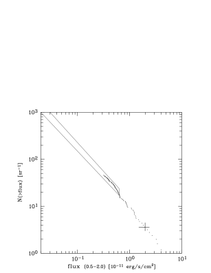
Figure 4.: (From De Grandi 1996). Left panel: Count rates for KP sources estimated through the “steepness ratio” method as a function of SASS count rates for the KP candidate cluster sources. The dashed lines show how an initial SASS count limit (CR_SASS), affects the corresponding true completeness limit in the corrected counts (CR). Open symbols correspond to core radii $<$ 60^′′, filled symbols to within 60^′′ and 120^′′, and crosses to values $>$ 120^′′. Right panel: the observed surface density of clusters of the resulting KP X–ray flux–limited pilot sample (dots). The error cross is the Piccinotti et al. (1982) result. The box shows the EMSS number counts as estimated by Rosati et al. (1995).

Redshift Survey Strategy and Early Results

The project will use a total of 90 nights, equally distributed among the 3.6 m, 2.2 m and 1.5 m ESO telescopes. We typically observe at least 5 galaxies per cluster, possibly more, to be able to disentangle the contamination from galaxy interlopers (e.g. Collins et al. 1995). In addition, with $N>5-10$ redshifts a reasonable estimate of the velocity dispersion can be obtained for most of the clusters. EFOSC at the 3.6 m telescope allows MOS spectroscopy over a $\sim 5^{\prime}\times 5^{\prime}$ field of view, with 10–20 redshifts per field typically secured at once on moderately distant and/or compact clusters, with 30–40 minute exposures. More nearby, looser systems, are instead surveyed with a long–slit spectrograph at the 2.2 m and 1.5 m telescopes. At the time these proceedings are published, the survey should have used more than 60% of the total telescope time allocated, with more than 250 new candidates observed to be added to other 300 already known cluster redshifts from the literature or other recent surveys. Observations of the flux–limited pilot subsample of 111 clusters have been virtually completed, and a study of its luminosity function is under way.

As typical of large survey projects, some of the most interesting results are those which are not expected in the initial plans. In the case of the KP, an example is the serendipitous detection of gravitational arcs on the short service images collected prior to the MOS spectroscopy (Edge et al. 1994; Schindler et al. 1995). The latest discovery in particular, RXJ 1347.5–1145, has been found to be the most luminous cluster known in the ROSAT (0.1–2.4 keV) band. A follow–up campaign of observations on this rather interesting object has been started, involving both ROSAT–HRI and ASCA observations in the X–ray, and ground–based NTT plus possibly HST imaging in the optical. Fig.5 shows the HRI data superimposed onto the red CCD image on which the arcs were originally discovered.

Figure 5.: Optical image in the R band of the ultraluminous X–ray cluster RXJ 1347.5-1145. The image side is 1.4 arcmin. The candidate gravitational arclets are marked by the arrows, with the two main structures North–East and South–West of the central galaxy. The superimposed contours show the X–ray emission as seen in a 15760 s exposure with the ROSAT HRI, with a resolution of about 5 arcseconds.

A Northern Redshift Survey of ROSAT Clusters

In the Northern hemisphere a redshift survey of ROSAT clusters is also being performed (see Böhringer 1994 for details). The identification of clusters in the Northern part of the RASS is complicated by the lack of an optical galaxy catalogue comparable in depth and quality to those obtained in the South from the scanning of the IIIaJ plates. The survey work is therefore presently limited to a sample selected on the basis of the SASS extension parameter, a criterion that at present cannot guarantee the selection of all the true RASS X–ray clusters within a certain region. It will be therefore necessary to complement the sample with a more general cluster identification work as soon as a good galaxy data base (e.g. the SDSS) becomes available in the Northern sky. There is a strong case for this, since in this way the Southern and Northern surveys could be homogenized and combined, providing a total sample with about 1500 clusters at a typical depth of $\sim 600$ $\;{\rm h}^{-1}\;{\rm Mpc}$. This would be more than invaluable for all those cosmological investigations requiring all–sky coverage, as e.g. the study of dipoles and peculiar motions.

See also http://www.merate.mi.astro.it/$\sim$guzzo/KP.html for further information.

Figure 6.: An Aitoff RA–DEC all–sky projection showing the location of the major galaxy and cluster survey projects discussed in the text.

5. Conclusions

I believe a good conclusion here is to say that we seem to live in a very fortunate and exciting epoch, with all these very promising projects due to finish by the end of the Millenium. In a few years most of the sky will be covered spectroscopically down to a typical depth of $\sim 600\;{\rm h}^{-1}\;{\rm Mpc}$ and the amount of data and information at our disposal will be increased by two orders of magnitude. I thought the best way to have the feeling of how the sky will be attacked during the forthcoming years was to try and condense all I have talked about in this review into a single picture. After some headache with SM, the result is shown in fig.6.

Acknowledgments.

I would like to thank all my collaborators in the various projects discussed here for the privilege of discussing our common work. I thank G. E. Zucca for useful discussions, D. Weinberg and M. Strauss for providing data and information on the SDSS, and C. Collins for providing information on the 2dF project. I am grateful to E. Molinari for help with the figures and to M. Strauss for the use of his SM macros.

References

Baugh, C.M., & Efstathiou, G.P., 1993, MNRAS, 265, 145

Böhringer, H., 1995, in Proc. of $17^{th}$ TEXAS Symposium, W. Voges et al. eds., The New York Academy of Sciences, in press

Böhringer, H., 1994, in Studying the Universe with Clusters of Galaxies, H. Böhringer and S. Schindler eds., MPE report 256, 93

Branchini, E., Guzzo, L., & Valdarnini, R., 1994, ApJ, 424, L5

Chincarini, G., & Rood, H.J., 1976, ApJ, 206, 30

Cole, S., Fisher, K.B., & Weinberg, D.H., 1994, MNRAS, 267, 785

Collins, C.A., Guzzo, L., Nichol, R.C., & Lumsden, S.L., 1995, MNRAS, 274, 1071

Davis, M. & Peebles, P. J. E., 1983, ApJ, 267, 456

De Grandi, S., 1996, Ph.D. Thesis, Università di Milano

De Grandi,S., Molendi, S., and Böhringer, H., 1995, in Proc. of $17^{th}$ TEXAS Symposium,[…], in press

Ebeling, H. 1993, PhD Thesis, Universität München, MPE Report 250

Edge, A.C., Böhringer, H., Guzzo, L. et al. , 1994, A&A, 289, L34.

Fisher, K. B., Davis, M., Strauss, M. A., Yahil, A. & Huchra, J. P., 1994, MNRAS, 267, 927

Geller, M.J., & Huchra, J.P., 1989, Science, 246, 897

Gunn, J.E., & Weinberg, D.H., 1995, in Wide–Field Spectroscopy and the Distant Universe, S.J. Maddox & A. Aragón–Salamanca eds., World Scientific (Singapore), p.3

Giovanelli, R., & Haynes, M.P., 1991, ARA&A, 29, 499

Giovanelli, R., Haynes, M.P, & Chincarini, G.L., 1986, ApJ, 300, 57

Guzzo, L., Böhringer, H., Briel, U., et al. (The KP Team), 1995, in Wide–Field Spectroscopy and the Distant Universe, […], p.205

Guzzo, L., Fisher, K.B., Strauss, M.S., Giovanelli, R., & Haynes, M.P., 1995, Astroph. Letters & Comm., in press

Heydon–Dumbleton, N.H., Collins, C.A., & MacGillivray, H.T., 1989, MNRAS, 238, 379

Hill, J.M., 1988, in Fiber Optics in Astronomy, S.C. Barden ed., PASP (San Francisco), p.77

Lin, H., 1995, Ph.D. Thesis, Harvard University

Lynden–Bell, D., 1971, MNRAS 155, 95

Loveday, J., Efstathiou, G., Peterson, B.A., & Maddox, S.J., 1992, ApJ, 400, 143

Marzke, R.O., Geller, M.J., da Costa, L.N., & Huchra, J.P., 1995, AJ, in press

Park, C., Vogeley, M.S., Geller, M.J., & Huchra, J.P., 1994, ApJ, 431, 569

Peebles, P.J.E., 1980, The Large Scale Structure of the Universe, Princeton University Press, (Princeton)

Piccinotti, G., et al., 1982, ApJ, 253, 485

Rood, H.J., 1988, ARA&A, 26, 245

Romer, A.K., et al. , 1994, Nature, 372, 75

Rosati, P., Della Ceca, R., Burg, R., Norman, C., & Giacconi, R., 1995, ApJ, 445, L11

Sandage, A., Tamman, G., & Yahil, A., 1979, ApJ, 232, 252

Sarazin, C., 1986, Rev. Mod. Phys., 58, 1

Shectman, S., et al., 1995, in Wide–Field Spectroscopy and the Distant Universe, […], p.98

Schindler, S., Guzzo, L., Ebeling, H., et al. , 1995, A&A, 299, L9.

Smoot, G. F. et al. , 1992, ApJ, 371, L1.

Strauss, M.A., & Willick, J.A., 1995, Phys. Rep., 261, # 5 & 6, 271

Sutherland, W.J., 1988, MNRAS, 234, 159

Taylor, K., 1995, in Wide–Field Spectroscopy …, p.15

Trümper, J. 1992, QJRAS, 33, 165

Tucker, D.L., 1994, Ph.D. Thesis, Yale University

Vettolani, G., Zucca, E., Cappi, A., et al. (The ESP Team), 1996, in preparation

Voges, W. 1992, in International Space Year, ESA ISY–3, p.91

Zucca, E., Vettolani, G., Cappi, A., et al. , 1996, in Observational Cosmology: from Galaxies to Galaxy Systems, Astroph. Letters & Comm., in press