THE ANGULAR POWER SPECTRUM OF THE 4 YEAR COBE DATA

Max Tegmark

Max-Planck-Institut für Physik, Föhringer Ring 6, D-80805 München;

email: max@mppmu.mpg.de

1 INTRODUCTION

Since their discovery (Smoot et al. 1992), fluctuations in the Cosmic Microwave Background Radiation (CMB) have emerged as possibly one of the most promising ways of measuring key cosmological parameters such as the Hubble constant $h$, the density parameter $\Omega$, the baryon fraction $\Omega_{b}$, the cosmological constant $\Lambda$, etc. As the angular power spectrum of the CMB, usually denoted $C_{\l}$, depends on about a dozen cosmological parameters (see e.g. White et al. 1994, Bond 1995a, Hu 1995, Steinhardt 1995 or Tegmark 1996b for recent reviews), accurate determination of this power spectrum by future experiments could be used to measure all these parameters simultaneously, with accuracies of a few percent or better (Jungman et al. 1996). Although we are still years away from attaining this goal, which would require mapping the CMB at high resolution over a large fraction of the sky, our knowledge of the power spectrum has been growing steadily over the last few years. The first year of COBE/DMR data (Smoot et al. 1992) indicated that the power spectrum was approximately scale-invariant $(n\sim 1)$ on the large angular scales ($\l\mathrel{\hbox to0.0pt{\lower 3.0pt\hbox{$\mathchar 536\relax$}\hss}\raise 2.0pt\hbox{$\mathchar 316\relax$}}30$) to which COBE is sensitive, and this conclusion has been confirmed by the FIRS and TENERIFE experiments (Ganga et al. 1994; Hancock et al. 1994). Ground- and balloon-based experiments have produced numerous measurements of the fluctuations on degree scales $(\l\sim 50-300)$, and although the situation is still far from clear, there is now some evidence that the power spectrum is larger in this $\l$-range than on COBE scales (e.g. Scott et al. 1995; Kogut & Hinshaw 1996). Recent results from the CAT experiment (Hancock et al. 1996; Scott et al. 1996) indicate that the power spectrum has fallen to lower values at $\l\sim 600$, which could be interpreted as there being a CDM-type “Doppler peak” around $\l\sim 300$.

Our knowledge of the power spectrum for $\l\mathrel{\hbox to0.0pt{\lower 3.0pt\hbox{$\mathchar 536\relax$}\hss}\raise 2.0pt\hbox{$\mathchar 318\relax$}}30$ is still quite limited, since the small patches of sky surveyed at high resolution so far give a large sample variance. On the largest angular scales, however, the situation is much better, since COBE has mapped the entire sky. Indeed, the signal-to-noise ratio in the 4 year COBE data (Bennett et al. 1996) is so good that the error bars on the $C_{\l}$-estimates for $\l\mathrel{\hbox to0.0pt{\lower 3.0pt\hbox{$\mathchar 536\relax$}\hss}\raise 2.0pt\hbox{$\mathchar 316\relax$}}10$ are now entirely dominated by cosmic variance. This means that (apart from reducing possible systematic errors and correcting for residual foreground contamination), these are the best estimates that mankind will ever be able to make of the large-scale power.

In view of this experimental progress, it is clearly worthwhile to estimate the power spectrum from the 4 year COBE data as accurately as possible. This is the purpose of the present Letter.

1.1 Power spectrum estimation with incomplete sky coverage

Pioneering work on the problem of power spectrum estimation from experimental data (Peebles 1973; Hauser & Peebles 1973) has recently been extended and applied to the 4 year COBE data (Wright et al. 1996, hereafter W96). When estimating power spectra, it is customary to place both vertical and horizontal error bars on the data points, as in e.g. Figure 3. The former represent the uncertainty due to noise and sample variance, and the latter reflect the fact that an estimate of $C_{\l}$ inadvertently also receives contributions from other multipole moments. In other words, the estimate of $C_{\l}$ is in fact a weighted average of a band of multipoles. The weights are referred to as the window function, and for the estimate of $C_{\l}$ to be a good one, we clearly want the window function to be centered on $\l$ with an r.m.s. width $\Delta\l$ that is as small as possible. As is well-known, incomplete sky coverage destroys the orthogonality of the spherical harmonics, and makes it impossible to attain perfect spectral resolution, $\Delta\l=0$. For typical ground- and balloon-based experiments probing degree scales, the relative spectral blurring $\Delta\l/\l$ tends to be of order unity, which makes it difficult to resolve details such as the number of Doppler peaks. A much better method is that used in W96, where the relative spectral resolution $\Delta\l/\l$ is brought down to the order of $25\%$ by using spherical harmonics. In Tegmark (1996a, hereafter T96), a method was presented for reducing these horizontal error bars still further, down to their theoretical minimum, which for a $20^{\circ}$ galactic cut was seen to be $\Delta\l\sim 1$.

1.2 The importance of high spectral resolution

Just as high spectral resolution is crucial in for instance absorption line studies (since it prevents interesting features from getting smeared out), it is also important when measuring the CMB power spectrum. The reason is that we cannot a priori assume that the power spectrum will be a simple smooth function. Indeed, there are non-standard cosmologies, such as “small universe” models with nontrivial spatial topology, that predict power spectra which on average have an $n\sim 1$ slope but contain bumps and wiggles that can only be resolved with a high spectral resolution (Stevens et al. 1993; de Oliveira-Costa & Smoot 1995). In addition, lowering the spectral resolution degrades information: broad window functions make the estimates of nearby multipoles highly correlated, so that the resulting power spectrum plot will contain fewer independent data points than one may naively expect.

The remainder of this Letter is organized as follows. In Section 2, the four year COBE data set is analyzed. In Section 3, the results are discussed and compared with those obtained with other methods such as the orthogonalized spherical harmonic method of Górski (1994, hereafter G94) and the signal-to-noise eigenmode methods of Bond (1995b, hereafter B95) and Bunn and Sugiyama (1995, hereafter BS95).

2 RESULTS

2.1 The method

How to extract the angular power spectrum from a CMB map with maximum spectral resolution is been described in detail in T96. We will apply this method to the 4 year data here exactly as it was applied to the 2 year COBE data in T96. Below we give merely a brief review of how the method works, referring the interested reader to T96 for technical details.

A simple estimate of the multipole $C_{\l}$ is obtained by taking a linear combination of all pixels, squaring it, and subtracting off the expected noise contribution. The weights in the linear combination are conveniently plotted as a sky map in the same way that we plot the data, and we usually refer to the set of weights as a weight function. It is easy to show that the expectation value of such an estimate is a linear combination of all the true multipoles. The coefficients in this linear combination are called the window function, a function of $\l$ (see the examples in Figure 2). In other words, given any weight function, there is a corresponding window function. The window function turns out to be simply the square of the spherical harmonic coefficients of the weight function, summed over $m$.

In the Hauser-Peebles method, the weight functions are chosen to be the spherical harmonics, but set equal to zero inside the galaxy cut and appropriately rescaled. A number of other weight functions have been employed in CMB analyses, for instance the orthogonalized spherical harmonics of G94 and the signal-to-noise eigenfunctions of B95 and BS95 (these functions were tailor made for the problem of efficient parameter estimation with likelihood analysis, not for power spectrum estimation). The method of T96 simply employs those weight functions that give the narrowest window functions possible, and it is shown that these functions can be found by solving a certain eigenvalue problem numerically. In the simplest version of the method (the version we use here — it has $\gamma=0$ as in T96), these functions are completely independent of any prior assumptions about the power spectrum, and are hence determined by the geometry of the galaxy cut alone.

What are these weight functions like? A sample weight function is plotted in T96 together with the corresponding spherical harmonic, and it is seen that they look quite similar far away from the galactic cut. The main difference is that the optimal weight functions approach zero smoothly at the edge, whereas a truncated spherical harmonic does not. As is discussed in further detail in T96, this absence of sharp edges in the weight functions is a key feature of the method, since sharp edges cause “ringing” in Fourier space (in the multipole domain), which corresponds to an unnecessarily wide window function.

To reduce error bars, a multipole is estimated as a weighted average of estimates of the above-mentioned simple type, just as in the Hauser-Peebles method where $C_{\l}$ is estimated by an average of the square amplitudes of the $(2\l+1)$ different spherical harmonic coefficients.

2.2 The data

The 53 and 90 GHz channels (A and B) of the COBE DMR 4 year data were combined into a single sky map by the standard minimum-variance weighting, pixel by pixel. We use the data set that was pixelized in galactic coordinates. After removing all pixels less than $20^{\circ}$ away from the galactic plane, 4016 pixels remain. As has become standard, we make no attempts to subtract galactic contamination outside the cut.

The resulting power spectrum is shown in Figure 1. A brute force likelihood analysis of the 4 year data set (Hinshaw et al. 1996) gives a best fit normalization of $Q_{rms,ps}=18.4\,{\rm\mu K}$ for a simple $n=1$ model, corresponding to the heavy horizontal line in the figure. If this model were correct, we would expect approximately $68\%$ of the data points to fall within the shaded $1-\sigma$ error region. As can be seen, the height of this region (the size of the vertical error bars) is dominated by cosmic variance for low $\l$ and by noise for large $\l$. At the cost of increasing $\Delta\l$, the variance can of course be reduced further by grouping multipoles together in bands and averaging them with minimum-variance weighting, as shown in figures 3 and 4 and in Table 1. We have followed W96 and chosen the eight multipole bands 2, 3, 4, 5-6, 7-9, 10-13, 14-19 and 20-30.

Band $$\langle\l\rangle$$

1 2.31 0.89 9.6 0.0 22.6

2 3.45 1.06 25.4 15.7 32.3

3 4.38 1.26 27.5 20.7 32.9

4 5.87 1.43 28.1 24.0 31.7

5 8.34 1.62 25.9 22.1 29.3

6 11.9 1.82 22.3 17.8 26.1

7 17.0 2.26 30.4 25.3 34.7

8 25.6 3.49 31.8 0.0 48.6

Table 1: The COBE power spectrum $\delta T\equiv[\l(\l+1)C_{\l}/2\pi]^{1/2}$ in $\mu K$.

For verification, 1000 mock COBE maps were generated for the model $n=1$, $Q_{rms,ps}=18.4\,{\rm\mu K}$ and piped through the data analysis software. As expected, the extracted multipoles were found to be unbiased estimates of the true multipoles, and the scatter was in agreement with the (analytic) error bars shown in the figures.

2.3 The window functions

The horizontal bars in Figure 1 are seen to be fairly independent of $\l$, just as expected — as discussed in detail in T96, the angular size of the two sky patches surviving the galaxy cut is $\Delta\theta\sim 1$ radian, and we expect $\Delta\l\sim 1/\Delta\theta\sim 1$. A typical window function is shown in Figure 2, and exhibits the following features that are common to all our window functions:

• For even $\l$, the window function vanishes for all odd multipoles, and vice versa. This happens because the galactic cut is symmetric about the galactic plane, and thus preserves the orthogonality between even and odd spherical harmonics, since they have opposite parity.

• The window function is for all practical purposes zero for multipoles below $\l-2$ and above $\l+2$.

• The central value is typically about three times as high as the two sidelobes.

The multipole $D_{\l}\equiv\l(\l+1)C_{\l}$ is thus typically estimated by something like $0.6D_{\l}+0.2D_{\l-2}+0.2D_{\l+2}$. This corresponds to all data points in Figure 1 being uncorrelated, with the exception that points separated by $\Delta\l=2$ have a correlation of order $55\%$ and points separated by $\Delta\l=4$ have a correlation of order $9\%$. Note that neighboring points are completely uncorrelated.

The only exception to the above is the window function for the quadrupole, $\l=2$: since it is required to vanish at $\l=0$, it picks up a non-negligible contribution from $\l=6$ instead.

3 DISCUSSION

We have computed the angular power spectrum of the 4 year COBE DMR data using the maximum resolution method of T96. The signal-to-noise ratio in the data is now so high that the error bars for $\l\mathrel{\hbox to0.0pt{\lower 3.0pt\hbox{$\mathchar 536\relax$}\hss}\raise 2.0pt\hbox{$\mathchar 316\relax$}}10$ are entirely dominated by cosmic variance. This means that, apart from future corrections due to better modeling of foregrounds and systematics, this is close to the best measurement of the low multipoles that mankind will ever be able to make, since cosmic variance could only be reduced by measurements in a different horizon volume.

The power spectrum in Figure 1 is seen to be consistent with an $n=1$, $Q_{rms,ps}=18.4\,{\rm\mu K}$ model. This model is close to the best-fit models found in the various two-parameter Bayesian likelihood analyses (e.g., Hinshaw et al. 1996, Górski et al. 1996, W96), which we can interpret as the best-fit straight line through the data points in Figure 1 being close to the horizontal heavy line. As has frequently been pointed out (see e.g. White & Bunn 1995), Bayesean methods by their very nature can only make relative statements of merit about different models, and never address the question of whether the best-fit model itself is in fact inconsistent with the data. As an absurd example, the best fit straight line to a parabola on the interval $[-1,1]$ is horizontal, even though this is a terrible fit to the data. It is thus quite reassuring that the power spectrum in Figure 1 not only has the right average normalization and slope, but that each and every one of the multipoles appear to be consistent with this standard best fit model.

3.1 Comparison with other results

A number of other linear techniques for CMB analysis have recently been applied to the COBE data. Both the orthogonalized spherical harmonics method (G94), the Karhunen-Loève (KL) signal-to-noise eigenmode method (B95, BS95), and the brute-force method (Tegmark & Bunn 1995, Hinshaw et al. 1996) were devised to solve a different problem than the one addressed here. If one is willing to parametrize the power spectrum by a small number of parameters, for instance a spectral index and an amplitude, then these methods provide an efficient way of estimating these parameters via a likelihood analysis. Why cannot the basis functions of these methods be used to estimate the angular power spectrum $C_{\l}$ directly, as they are after all orthogonal over the galaxy-cut sky? The answer is that these basis functions are orthogonal to each other, whereas in our context, we want them to be as orthogonal as possible not to each other but to the spherical harmonics. This is illustrated in Figure 2, which contrasts $\l=20$ window functions of the optimal method and the generalized Hauser-Peebles method (W96, de Oliveira-Costa & Smoot 1995). We want the window function to be centered on $\l=20$, and be as narrow as possible, so the lower one is clearly preferable. The upper weight function is seen to couple strongly to many of the lower multipoles, and picks up a contribution from the quadrupole that is even greater than that from $\l=20$. This of course renders it inappropriate for estimating the power at $\l=20$. Analogous window functions can readily be computed for the orthogonalized spherical harmonics of G94 or the signal-to-noise eigenmodes of B95 and BS95. They are also broader than the optimal one in Figure 2 — the optimal weight functions of course give narrower window functions than other basis functions by definition, since they were defined as those functions that give the narrowest window functions possible.

It should be emphasized that generating such window functions for the basis functions of G94, B95 and BS95 would be quite an unfair criticism of these methods, since this would be grading them with respect to a property that they were not designed to have. These authors have never claimed that their basis functions were optimal for multipole estimation, merely (and rightly so) that they were virtually optimal for parameter fitting with a likelihood analysis.

The power spectrum of Figure 1 is also consistent with that extracted in W96 using the Hauser-Peebles method. At low $\l$, the individual multipoles estimates agree well with each other. As $\l$ increases, the spectral resolution $\Delta\l$ of the Hauser-Peebles method grows approximately linearly (see T96) whereas the resolution in Figure 1 is seen to more or less remain constraint. Thus the data points in $W96$ begin to differ from those in Figure 1 at larger $\l$, since the former are no longer probing individual multipoles but weighted averages of a broad range.

In summary, the 4 year COBE data has measured the power spectrum for $\l\mathrel{\hbox to0.0pt{\lower 3.0pt\hbox{$\mathchar 536\relax$}\hss}\raise 2.0pt\hbox{$\mathchar 316\relax$}}15$ with an accuracy approaching the cosmic variance limit. As the next generation of CMB experiments extend this success to smaller angular scales, the CMB may turn out to be one of the most potent arbiters between cosmological models.

The author wishes to thank Angélica de Oliveira-Costa, Krystof Górski, Ned Wright and an anonymous referee for helpful comments on the manuscript. This work was partially supported by European Union contract CHRX-CT93-0120 and Deutsche Forschungsgemeinschaft grant SFB-375. The COBE data sets were developed by the NASA Goddard Space Flight Center under the guidance of the COBE Science Working Group and were provided by the NSSDC.

4 REFERENCES

Bennett, C. L. et al. 1996, ApJ, 464, L1.

Bond, J. R. 1995a, in Cosmology and Large Scale Structure, ed. Schaeffer, R. (Elsevier).

Bond, J. R. 1995b, Phys. Rev. Lett., 74, 4369 (“B95”).

Bunn, E. F. & Sugiyama, N. 1995, ApJ, 446, 49 (“BS95”).

de Oliveira-Costa, A. & Smoot, G. F. 1995, ApJ, 448, 477.

Ganga, K. et al. 1994, ApJ, 432, L15.

Górski 1994, ApJ, 430, L85 (“G94”).

Górski et al. 1996, ApJ, 464, L11.

Hancock, S. et al. 1994, Nature, 367, 333.

Hancock, S. et al. 1996, submitted to Nature.

Hauser, M. G. & Peebles, P. J. E. 1973, ApJ, 185, 757.

Hinshaw, G. et al. 1996;464;L17

Hu, W. 1995, in The Universe at High-z, eds. E. Martinez-Gonzalez and J.L. Sanz (Springer, in press), astro-ph/9511130.

Jungman et al. 1996, preprint astro-ph/9512139.

Kogut, A. et al. 1996, ApJ, 464, L5.

Kogut, A. & Hinshaw, G. 1996, ApJ, 464, L39.

Netterfield, C. B. et al. 1996, preprint astro-ph/9601197.

Peebles, P. J. E. 1973, ApJ, 185, 413.

Scott D, Silk J and White M 1995, Science, 268, 829.

Scott et al. 1996, in preparation.

Smoot, G.F. et al. 1992, ApJ, 396, L1.

Steinhardt P S 1995, preprint astro-ph/9502024.

Stevens, D., Scott, D. & Silk, J. 1993, Phys. Rev. Lett., 71, 20.

Sugiyama, N. 1995, ApJS, 100, 281.

Tegmark, M. & Bunn, E. F. 1995, ApJ, 455, 1.

Tegmark, M. 1996a, MNRAS, 280, 299.

(“T96”).

Tegmark, M. 1996b, to appear in Proc. Enrico Fermi, Course CXXXII, Varenna, eds. Bonometto, S. & Primack, J., astro-ph/9511148.

White, M. & Bunn, E. F. 1995, ApJ, 450, 477.

White, M., Scott, D. and Silk, J. 1994, ARA&A, 32, 319.

Wright, E. L. et al. 1996, ApJ, 464, L21 (“W96”).

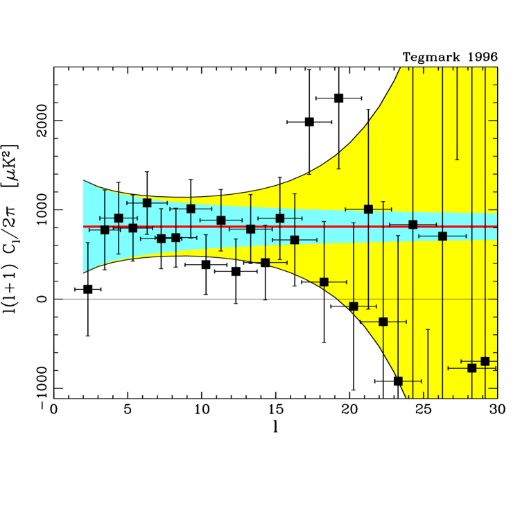
Figure 1: The power spectrum observed by COBE.

The observed multipoles $D_{\l}=\l(\l+1)C_{\l}$ are plotted with $1-\sigma$ error bars. The vertical error bars include both pixel noise and cosmic variance, and the horizontal bars show the width of the window functions used. If the true power spectrum is given by $n=1$ and $Q_{rms,ps}=18.4{\rm\mu K}$ (the heavy horizontal line), then the shaded region gives the $1-\sigma$ error bars and the dark-shaded region shows the contribution from cosmic variance.

Figure 2: Window functions before and after optimization.

Two window functions for estimation of the multipole $\l=20$, $m=0$ are shown. The upper one is that of the spherical harmonic method (W96), which exhibits a strong leakage from lower multipoles such as the quadrupole. The lower one is the one resulting from the optimal method.

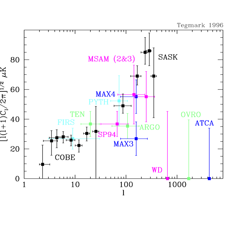
Figure 3: Power spectrum measurements.

The observed multipoles $D_{\l}=\l(\l+1)C_{\l}$ are plotted for a selection of experiments. Both vertical and horizontal bars have the same meaning as in Figure 1. The COBE data are those of Figure 1, averaged over 8 multipole bands, and the rest are from the Saskatoon experiment (Netterfield et al. 1996) and from the compilation of Scott et al. (1995).

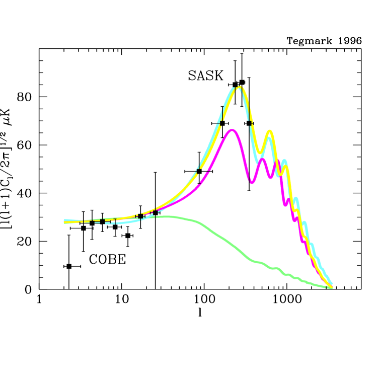
Figure 4: Power spectrum models.

The data points from Figure 3 with the narrowest window functions (COBE and Saskatoon) are compared with the predictions from four variants of the standard CDM model from Sugiyama (1995), all with $n=1$ and $\Omega_{b}=0.05$. From top to bottom at $\l=200$, they are a flat model with $\Lambda=0.7$, a model with $h=0.3$, the standard $h=0.5$ model and a model with a reionization optical depth $\tau\sim 2$.