Cosmic Microwave Background non–Gaussian signatures
from analytical texture models

Abstract

Using an analytical model for the Cosmic Microwave Background anisotropies produced by textures, we compute the resulting collapsed three–point correlation function and the rms expected value due to the cosmic variance. We apply our calculations to the COBE–DMR experiment and test the consistency of the model with the observational results. We also show that an experiment with smaller angular resolution can put bounds to the model parameters.

I Introduction

An important problem in cosmology is that of finding out the source of the density perturbations leading to the large scale structure formation. Competing models are inflationary scenarios and topological defects, these latter formed as the consequence of a symmetry breaking phase transition in the early universe.

A possible way of trying to discriminate between models is given by the anisotropies in the Cosmic Microwave Background (CMB) radiation predicted by them. In inflationary models, large scale anisotropies arise from the Sachs–Wolfe effect [1] and are proportional to the fluctuations of the gravitational potential on the last–scattering surface. These are generated as a result of quantum fluctuations of scalar fields during inflation. The resulting anisotropies are consistent with the analysis of the two–point correlation function of the two–year COBE–DMR data [2], which fixes the amplitude of the power spectrum and constrains the spectral index, provided that the couplings of the inflaton field are very weak. As a consequence, the CMB anisotropies produced in inflationary models are nearly Gaussian distributed.

Defect–induced large scale structure formation has been well studied recently [3, 4, 5, 6] and its predictions confront successfully against a large bulk of observational data. The amplitude of the anisotropies, which can be determined using the COBE–DMR data, is directly related to the symmetry breaking energy scale and corresponds to a Grand Unification Theory (GUT) phase transition. However, the production of anisotropy maps from numerical simulations of the field equations turns out to be a fabulous task, and therefore some analytical insight is desirable. This is the reason why people turned to consider analytical (although simplified) models for CMB anisotropies generated by defects, wherein the physics is more transparent and computations can be pursued straightforwardly [7, 8, 9]. Although it is clear that full range numerical simulations will have the last word regarding these and other observable signatures of defects, in the meantime progress with these simplified models can hint some of their main features.

CMB maps contain more information than the one that can be extracted by studying just the two–point correlation function. Recently, Hinshaw et al. [10] analysed the three–point function of the two–year COBE–DMR data and found a non–vanishing signal, although consistent with the level of cosmic variance associated to a Gaussian process. The predictions for the three–point CMB function in inflationary models have recently been worked out in detail. The contribution coming from the non–linearities in the inflaton evolution and in the relation between the inflaton fluctuations and the CMB resulting anisotropies have been computed in Refs. [11, 12, 13]. Also the post recombination mildly non–linear evolution of the perturbations gives rise to a non–vanishing contribution through the Rees–Sciama effect [14, 15, 16]. Both contributions result to be more than three orders of magnitude smaller than the associated cosmic variance, and are thus consistent with the COBE–DMR data. It is interesting to know whether the predictions of topological defect models are also consistent with the COBE–DMR three–point function data or not. As defects are the typical example of non–Gaussian perturbation sources, the resulting three–point function and its cosmic variance can easily differ from the Gaussian ones. In this paper we apply a recently proposed analytical model of anisotropies produced by textures [8] to study the predictions for the three–point correlation function and cosmic variance of the CMB and we compare this theoretical band with the COBE–DMR data.

As an example that this statistics can be a useful test for models of structure formation, let us note that, based on the analysis of the three–point function of the COBE–DMR data, Hinshaw et al. [10] were able to rule out an inflationary model for primordial isocurvature baryon (PIB) fluctuations proposed by Yamamoto and Sasaki [17]. In this model the predicted mean skewness vanishes and the rms skewness (cosmic variance) results several orders of magnitude below the standard adiabatic models one, and the authors suggest that the rms value of the full three–point function would be tiny as well. This would make the theoretical error bars for the three–point function predicted by this PIB model smaller that the actual data from the maps, hence running into conflict with the result of the COBE–DMR analysis.

Likewise, it is interesting to check whether the non–Gaussian signatures predicted by the analytical texture model are in agreement with the analyses of the maps, and if not what the constraints are. This is the main aim of the present paper.

II The collapsed three–point correlation function

The three–point correlation function for points at three arbitrary angular separations $\alpha$, $\beta$ and $\gamma$ is given by the average product of temperature fluctuations in all possible three directions with those angular separations among them [12]. In this paper, for simplicity, we will restrict ourselves to the collapsed case, corresponding to the choice $\alpha=\beta$ and $\gamma=0$, that is one of the cases analysed for the COBE–DMR data [18, 10] (the other is the equilateral one, $\alpha=\beta=\gamma$). The collapsed three–point correlation function of the CMB is given by

$$C_{3}(\alpha)\equiv\int\frac{d\Omega_{\hat{\gamma}_{1}}}{4\pi}\int\frac{d\Omega_{\hat{\gamma}_{2}}}{2\pi}\Delta T(\hat{\gamma}_{1})\Delta T^{2}(\hat{\gamma}_{2})\delta(\hat{\gamma}_{1}\cdot\hat{\gamma}_{2}-\cos\alpha).$$ (1)

For $\alpha=0$, we recover the well–known expression for the skewness, $C_{3}(0)$. By expanding the temperature fluctuations in spherical harmonics ${\Delta T\over T}(\vec{x},\hat{\gamma})=\sum_{\ell,m}a_{\ell}^{m}(\vec{x})Y_{\ell}^{m}(\hat{\gamma})$, we can write the collapsed three–point function as

$$C_{3}(\alpha)=\frac{T_{0}^{3}}{4\pi}\sum_{\ell_{1},\ell_{2},\ell_{3},m_{1},m_{2},m_{3}}P_{\ell_{1}}(\cos\alpha)a_{\ell_{1}}^{m_{1}}a_{\ell_{2}}^{m_{2}}a_{\ell_{3}}^{m_{3}}{\cal W}_{\ell_{1}}{\cal W}_{\ell_{2}}{\cal W}_{\ell_{3}}\bar{\cal H}_{\ell_{1}\ell_{2}\ell_{3}}^{m_{1}m_{2}m_{3}}~{},$$ (2)

where $T_{0}=2.726\pm 0.01$K is the mean temperature of the CMB radiation [19], ${\cal W_{\ell}}$ represents the window function of the particular experiment and we follow the notation in Ref. [12], defining

$$\bar{\cal H}_{\ell_{1}\ell_{2}\ell_{3}}^{m_{1}m_{2}m_{3}}\equiv\int d\Omega_{\hat{\gamma}}Y_{\ell_{1}}^{m_{1}}(\hat{\gamma})Y_{\ell_{2}}^{m_{2}}(\hat{\gamma})Y_{\ell_{3}}^{m_{3}}(\hat{\gamma})~{},$$ (3)

which have a simple expression in terms of Clebsh–Gordan coefficients.

Predictions from different models usually come as expressions for the ensemble average of the angular bispectrum $\bigl{\langle}a_{\ell_{1}}^{m_{1}}a_{\ell_{2}}^{m_{2}}a_{\ell_{3}}^{m_{3}}\bigr{\rangle}$, from which we obtain the predicted $\langle C_{3}(\alpha)\rangle$. This corresponds to the mean value expected in an ensemble of realizations. However, as we can observe just one particular realization, we have to take into account the spread of the distribution of the three–point function values when comparing a model prediction with the observational results. This is the well–known cosmic variance problem [20, 21]. We can estimate the range of expected values about the mean by the rms dispersion

$$\sigma_{CV}^{2}(\alpha)\equiv\bigl{\langle}C_{3}^{2}(\alpha)\bigr{\rangle}-\bigl{\langle}C_{3}(\alpha)\bigr{\rangle}^{2}.$$ (4)

III CMB anisotropies from Textures

CMB anisotropies in defect theories are produced during the photon travel all the way from the last scattering surface to here. The computation is quite involved because it requires simulations following the defects, matter and photon evolution over a large number of expansion times [4, 5, 6, 22]. In the case of textures, the non–linear evolution of the scalar field responsible for texture formation is the source of the CMB anisotropies. As long as the characteristic length scale of these defects is larger than the Hubble radius $H^{-1}$ the gradients of the field are frozen in and cannot affect the surrounding matter components. However, when the size of the texture becomes comparable to $H^{-1}$ (this latter grows linearly with cosmic time), microphysical processes can ‘push’ the global fields so that they acquire trivial field configurations, reduce their energy (which is radiated away as Goldstone bosons) and, in those cases where the field was wounded in knots, they unwind. In this process perturbations in the spacetime metric are generated, and hence also the photon geodesics are affected. These unwinding events are mainly characterised by one length scale, that of the Hubble radius at the moment of collapse, implying that the resulting perturbations arise at a fixed rate per Hubble volume and Hubble time. This scaling property means that the defect network looks statistically the same at any time, once its characteristic length is normalised to $H^{-1}$. Then, by dividing the sky cone into cells corresponding to expansion times and Hubble volumes, one can restrict to the study of the CMB pattern induced in Hubble–size boxes during one Hubble time. Such studies have been performed by Borrill et al. [23] and Durrer et al. [24]. In the latter paper, a ‘scaling–spot–throwing’ process was implemented numerically, with CMB spots derived from a self–similar and spherically symmetric model of texture collapse [25, 26].

An analytical approach to compute the multipole coefficients ${\cal C}_{\ell}$, the two–point function, and the cosmic variances for CMB anisotropies arising in texture models have recently been proposed by Magueijo [8]. The model allows to study texture–induced spots of arbitrary shapes and relies on a hand–full of ‘free’ parameters to be specified by numerical simulations, like the number density of spots, $\nu$, the scaling size, $d_{s}$, and the brightness factor of the particular spot, $a_{k}$, which tells us about its temperature relative to the mean sky temperature (in particular, its sign indicates whether it is a hot or a cold spot).

Let us start by discussing the spots statistics. Texture configurations giving rise to spots in the CMB are assumed to arise with a constant probability per Hubble volume and Hubble time. By dividing the whole volume in boxes of surface $dS$ and thickness $d\ell$ we may write the volume probability density of spot generation in the sky as follows

$$d{\cal P}={\nu\over H^{-4}}dSd\ell dt$$ (5)

FIG. 1.: Texture–induced hot and cold spots produced on different Hubble volumes and Hubble times, from the last scattering surface to today (see text). Dashed arrows indicate three possible directions on the microwave sky. The angle $\alpha$ corresponds to that in the collapsed three–point correlation function $C_{3}(\alpha)$.

where $\nu$ is the mean number of CMB spots expected to be produced in a Hubble volume and in a Hubble time. Now, we are interested in a two dimensional distribution of spots (since observations map the two dimensional sky sphere), and thus we may integrate the thickness $d\ell$ in an interval of order $H^{-1}$ to get the surface probability density

$$dP\simeq{\nu\over H^{-3}}dSdt~{}.$$ (6)

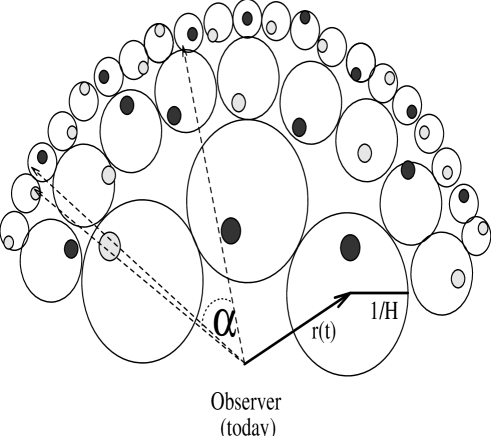
Taking into account the expansion of the universe we may express $dS=r^{2}(t)d\Omega$, with $r(t)=3t((t_{0}/t)^{1/3}-1)$, where $t$ denotes proper time and $t_{0}$ stands for its value today. It is convenient to change the time variable to $y(t)\equiv\log_{2}(t_{0}/t)$, which measures how many times the Hubble radius has doubled since time $t$ up to now (see Fig. 1). For a redshift $z_{\rm ls}\sim 1400$ at last scattering we have $y_{\rm ls}\simeq\log_{2}[(1400)^{3/2}]\simeq 16$. In terms of $y$ the surface probability density may be cast as

$$dP=N(y)dyd\Omega,$$ (7)

with

$$N(y)=-{8\nu\ln(2)\over 3}\left(2^{y/3}-1\right)^{2}~{}.$$ (8)

Within the model, CMB anisotropies arise from texture–induced spots in the sky. Thus, we may express the anisotropies as the superposition of the contribution coming from all the individual spots $S_{k}$ produced from $y_{\rm ls}$ up to now,

$${\Delta T\over T}=\sum_{k}a_{k}S_{k}(\theta_{k},y).$$ (9)

In this expression, $a_{k}$ describes the brightness of the hot/cold $k$–th spot and is interpreted as a random variable, which characteristic values have to be extracted from numerical simulations as those of Ref. [23]. $S_{k}(\theta_{k},y)$ is the characteristic shape of the spots produced at time $y$, where $\theta_{k}$ is the angle in the sky measured with respect to the center of the spot.

A spot appearing at time $y$ has typically a size $\theta^{s}(y)\simeq d_{s}~{}\theta^{\rm hor}(y)$, with $\theta^{\rm hor}(y)$ the angular size of the horizon at $y$, and where

$$\theta^{s}(y)=\arcsin\left({d_{s}H^{-1}\over r(t)}\right)=\arcsin\left({0.5d_{s}\over 2^{y/3}-1}\right)~{}.$$ (10)

As spot anisotropies are generated by causal seeds, their angular size cannot exceed the size of the horizon at that time and thus $d_{s}\leq 1$. The scaling hypothesis implies that the profiles satisfy $S_{k}(\theta_{k},y)=S(\theta_{k}/\theta^{s}(y))$.

Combining the expression for $\Delta T/T$ in Eq. (9) and its expansion in spherical harmonics, we easily find the expression for the multipole coefficients $a_{\ell}^{m}$ in terms of the brightness and the profile of the spots

$$a_{\ell}^{m}=\sum_{k}a_{k}S^{\ell}_{k}(y){Y_{\ell}^{m}}^{*}(\hat{\gamma}_{k})~{},$$ (11)

where

$$S^{\ell}_{k}(y)=2\pi\int_{-1}^{1}S_{k}(\theta_{k},y)P_{\ell}(\cos\theta_{k})d\cos\theta_{k}~{}.$$ (12)

We can now compute the angular spectrum predicted within this analytical model

$${\cal C}_{\ell}\equiv{T_{0}^{2}\over(2\ell+1)}\sum_{m=-\ell}^{\ell}\langle|a_{\ell}^{m}|^{2}\rangle={T_{0}^{2}\over(2\ell+1)}\sum_{m=-\ell}^{\ell}\sum_{kk^{\prime}}\langle a_{k}a_{k^{\prime}}S_{k}^{\ell}S_{k^{\prime}}^{\ell}\rangle Y_{\ell}^{m}(\hat{\gamma}_{k}){Y_{\ell}^{m}}^{*}(\hat{\gamma}_{k^{\prime}})~{},$$ (13)

where $\bigl{\langle}\cdot\bigr{\rangle}$ denotes ensemble average. Any two different texture–spots are uncorrelated, hence we have

$$\bigl{\langle}a_{k}a_{k^{\prime}}S_{k}^{\ell}S_{k^{\prime}}^{\ell}\bigr{\rangle}=\delta_{kk^{\prime}}a_{k}^{2}\left(S_{k}^{\ell}\right)^{2}~{}.$$ (14)

Thus,

$${\cal C}_{\ell}={T_{0}^{2}\over 4\pi}\sum_{k}a_{k}^{2}\left(S_{k}^{\ell}\right)^{2}~{}.$$ (15)

The sum over all the spots contributing to the $\Delta T/T$ is performed by integrating this expression with the probability function in Eq. (7), we obtain

$${\cal C}_{\ell}=T_{0}^{2}\bigl{\langle}a^{2}\bigr{\rangle}{\cal I}_{2}^{\ell\ell}~{},$$ (16)

where we defined

$${\cal I}_{D}^{\ell_{1}\ldots\ell_{D}}\equiv\int dyN(y)S^{\ell_{1}}(y)\ldots S^{\ell_{D}}(y)~{}.$$ (17)

$\bigl{\langle}a^{2}\bigr{\rangle}$ in Eq. (16) is the mean squared value of the spot brightness, to be computed from the distribution {$a_{k}$} resulting from simulations.

IV Texture three–point function

Let us now compute the angular bispectrum. Following the same steps as in the previous section we may express it as

$$\bigl{\langle}a_{\ell_{1}}^{m_{1}}a_{\ell_{2}}^{m_{2}}a_{\ell_{3}}^{m_{3}}\bigr{\rangle}=\bigl{\langle}a^{3}\bigr{\rangle}{\cal I}_{3}^{\ell_{1}\ell_{2}\ell_{3}}\bar{\cal H}_{\ell_{1}\ell_{2}\ell_{3}}^{m_{1}m_{2}m_{3}}~{}.$$ (18)

This time the angular integral in the probability (Eq. (7)) is the responsible for the appearance of the factor $\bar{\cal H}_{\ell_{1}\ell_{2}\ell_{3}}^{m_{1}m_{2}m_{3}}$. Replacing this expression in Eq. (2) we obtain the mean collapsed three–point function predicted by this model

$$\bigl{\langle}C_{3}(\alpha)\bigr{\rangle}={\bigl{\langle}a^{3}\bigr{\rangle}T_{0}^{3}\over(4\pi)^{2}}\sum_{\ell_{1},\ell_{2},\ell_{3}}(2\ell_{1}+1)(2\ell_{2}+1)(2\ell_{3}+1)P_{\ell_{1}}(\cos\alpha){\cal W}_{\ell_{1}}{\cal W}_{\ell_{2}}{\cal W}_{\ell_{3}}{\cal I}_{3}^{\ell_{1}\ell_{2}\ell_{3}}{\cal F}_{\ell_{1}\ell_{2}\ell_{3}}~{},$$ (19)

where ${\cal F}_{\ell_{1}\ell_{2}\ell_{3}}\equiv\left({}^{\ell_{1}~{}\ell_{2}~{}\ell_{3}}_{0~{}~{}0~{}~{}0}\right)^{2}$ are just the squares of the the $3j$–symbols [27].

The other quantity of interest is the expected rms dispersion about the three–point function due to the cosmic variance, given by Eq. (4). Computing the ensemble average of the combination of six $a_{\ell}^{m}$’s, $\bigl{\langle}a_{\ell_{1}}^{m_{1}}\ldots a_{\ell_{6}}^{m_{6}}\bigr{\rangle}$, and replacing it into the expression of $\sigma_{CV}^{2}(\alpha)$, we obtain after a lengthy calculation

$$\sigma_{CV}^{2}(\alpha)=$$ (27)

$$2~{}{\bigl{\langle}a^{2}\bigr{\rangle}^{3}T_{0}^{6}\over(4\pi)^{3}}\!\!\sum_{\ell_{1},\ell_{2},\ell_{3}}\!\!P_{\ell_{1}}(\alpha)(P_{\ell_{1}}(\alpha)\!+\!P_{\ell_{2}}(\alpha)\!+\!P_{\ell_{3}}(\alpha))~{}{\cal F}_{\ell_{1}\ell_{2}\ell_{3}}\prod_{\ell=\ell_{1}}^{\ell_{3}}{\cal I}_{2}^{\ell\ell}{\cal W}_{\ell}^{2}(2\ell+1)$$

$$+{\bigl{\langle}a^{2}\bigr{\rangle}\bigl{\langle}a^{4}\bigr{\rangle}T_{0}^{6}\over(4\pi)^{4}}\sum_{\ell_{1},\ell_{2},\ell_{3},\ell_{5},\ell_{6}}\left[P_{\ell_{1}}^{2}(\alpha)+4P_{\ell_{1}}(\alpha)P_{\ell_{2}}(\alpha)+4P_{\ell_{2}}(\alpha)P_{\ell_{5}}(\alpha)\right]$$

$$\times{\cal I}_{2}^{\ell_{1}\ell_{1}}{\cal I}_{4}^{\ell_{2}\ell_{3}\ell_{5}\ell_{6}}~{}{\cal W}^{2}_{\ell_{1}}{\cal W}_{\ell_{2}}{\cal W}_{\ell_{3}}{\cal W}_{\ell_{5}}{\cal W}_{\ell_{6}}~{}{\cal F}_{\ell_{1}\ell_{2}\ell_{3}}{\cal F}_{\ell_{1}\ell_{5}\ell_{6}}(2\ell_{1}+1)(2\ell_{2}+1)(2\ell_{3}+1)(2\ell_{5}+1)(2\ell_{6}+1)$$

$$+{\bigl{\langle}a^{3}\bigr{\rangle}^{2}T_{0}^{6}\over(4\pi)^{4}}\sum_{\ell_{1},\ell_{2},\ell_{3},\ell_{5},\ell_{6}}\left[P_{\ell_{1}}^{2}(\alpha)+4P_{\ell_{1}}(\alpha)P_{\ell_{2}}(\alpha)+4P_{\ell_{2}}(\alpha)P_{\ell_{5}}(\alpha)\right]$$

$$\times{\cal W}_{\ell_{1}}^{2}{\cal W}_{\ell_{2}}{\cal W}_{\ell_{3}}{\cal W}_{\ell_{5}}{\cal W}_{\ell_{6}}{\cal I}_{3}^{\ell_{1}\ell_{2}\ell_{3}}{\cal I}_{3}^{\ell_{1}\ell_{5}\ell_{6}}{\cal F}_{\ell_{1}\ell_{2}\ell_{3}}{\cal F}_{\ell_{1}\ell_{5}\ell_{6}}(2\ell_{1}+1)(2\ell_{2}+1)(2\ell_{3}+1)(2\ell_{5}+1)(2\ell_{6}+1)$$

$$+{\bigl{\langle}a^{6}\bigr{\rangle}T_{0}^{6}\over(4\pi)^{5}}\sum_{\ell_{1},\ell_{2},\ell_{3},\ell_{4},\ell_{5},\ell_{6}}P_{\ell_{1}}(\alpha)P_{\ell_{4}}(\alpha)~{}{\cal W}_{\ell_{1}}{\cal W}_{\ell_{2}}{\cal W}_{\ell_{3}}{\cal W}_{\ell_{4}}{\cal W}_{\ell_{5}}{\cal W}_{\ell_{6}}{\cal I}_{6}^{\ell_{1}\ell_{2}\ell_{3}\ell_{4}\ell_{5}\ell_{6}}$$

$$\times{\cal F}_{\ell_{1}\ell_{2}\ell_{3}}{\cal F}_{\ell_{4}\ell_{5}\ell_{6}}(2\ell_{1}+1)(2\ell_{2}+1)(2\ell_{3}+1)(2\ell_{4}+1)(2\ell_{5}+1)(2\ell_{6}+1)~{}.$$

We can estimate the range for the amplitude of the three–point correlation function predicted by the model by $\bigl{\langle}C_{3}(\alpha)\bigr{\rangle}\pm\sigma_{CV}(\alpha)$.

Let us note that a brightness distribution {$a_{k}$} symmetric in hot and cold spots implies $\bigl{\langle}a^{3}\bigr{\rangle}=0$ and therefore yields a vanishing three–point function. This is precisely what happens for spots generated by spherically symmetric self–similar (SSSS) texture unwinding events [25]. However, the properties of the SSSS solution are not characteristic of spot arising from more realistic random configurations. Borrill et al. [23] have shown that randomly generated texture field configurations produce anisotropy patterns with very different properties to the exact SSSS solution. Furthermore, spots generated from concentrations of energy gradients which do not lead to unwinding events can still produce anisotropies very similar to those generated by unwindings. The peak anisotropy of the random configurations turns out to be 20 to 40 % smaller than the SSSS solution. Moreover, their results also suggest an asymmetry between maxima $\langle a_{\rm max}\rangle$ and minima $\langle a_{\rm min}\rangle$ of the peaks for all studied configurations other than the SSSS, although with large error bars. They justify this result as due to the fact that, for unwinding events, the minima are generated earlier in the evolution (photons climbing out of the collapsing texture) than the maxima (photons falling in the collapsing texture), and thus the field correlations are stronger for the maxima, which enhance the anisotropies.

V Numerical results

Up to this point we have left unspecified the profile of the spots, the distribution of the brightness factor $\{a_{k}\}$, the typical size of the spots $d_{s}$ and the number density of spots $\nu$. We have to fix them in order to obtain a quantitative estimate of the three–point function and the cosmic variance. We will essentially rely on the results of the simulations of Ref. [23], where all these issues are addressed to some extent. These simulations indicate that the size of the spots are approximately 10% of the Hubble radius when generated, hence we take the scaling size $d_{s}\simeq 0.1$. There is no particular form of the spot profiles obtained in the simulations. However, a Gaussian function, as given by the profile $S(\theta/\theta_{s}(y))\propto\exp(-\theta^{2}/\theta^{2}_{s}(y))$ looks as a good approximation to the bell–shaped spots obtained in Ref. [23] and we will adopt it here for the numerical computations. Another interesting result obtained in Ref. [23] regards the number of spots produced: whereas only 4 out of 100 simulations showed unwinding events, the number density of nonunwinding events (which as we mentioned above also lead to spots) is much greater, typically of the order of one such event per simulation. This implies a mean number of CMB spots per Hubble volume and Hubble time $\nu\simeq 1$.

We need also the distribution of the spot brightness $\{a_{k}\}$ in order to compute the mean values of the powers of the random variable $a$, $\langle a^{n}\rangle$, appearing in Eqs. (19) and (27). As we do not have at our disposal the full distribution of values obtained in the simulations and we just know the mean value of the maxima and the minima, we will make a crude estimate by considering that all the hot spots appear with the same $a_{h}>0$ and all the cold spots with the same $a_{c}<0$. Then, all the $\langle a^{n}\rangle$ needed can readily be obtained in terms of $\langle a^{2}\rangle$ and $x\equiv\langle a\rangle/\langle|a|\rangle$. From the two–point correlation function of the COBE–DMR data, we can normalize the amplitude of the anisotropies and fix $\langle a^{2}\rangle$. We do this by fixing ${\cal C}_{9}=(8\mu{\rm K})^{2}$ [28] which, with the help of Eq. (16), leads to $\langle a^{2}\rangle(T_{0})^{2}=1.4\times 10^{5}\mu{\rm K}^{2}$. The other parameter, $x$, measures the possible asymmetry between hot and cold spots and we leave it as a free parameter. Let us note that the amplitude of the spots is directly related to the scale of symmetry breaking. From Ref. [23], $\langle a^{2}\rangle^{1/2}\simeq 0.7\epsilon$, with $\epsilon=8\pi^{2}G\Phi_{0}^{2}$. Hence, the symmetry breaking scale results $\Phi_{0}\simeq 1.6\times 10^{-3}m_{P}$, typical of GUT theories.

We may now apply our formalism to the COBE–DMR measurements. We consider a Gaussian window function, ${\cal W}_{\ell}\simeq\exp(-\ell(\ell+1)\sigma^{2}/2)$, with dispersion of the antenna beam profile $\sigma=3.2^{\circ}$ [29]. The analytical formulae obtained in the previous section assumed full–sky coverage. The effect of partial coverage, due to the cut in the maps at Galactic latitudes $|b|<20^{\circ}$, increases the cosmic variance by a factor $\sim 1.56$ [18], and we take it into account by multiplying $\sigma_{CV}$ by this factor in the numerical results.

FIG. 2.: Collapsed three–point function $\bigl{\langle}C_{3}(\alpha)\bigr{\rangle}$ (solid line) and the rms cosmic variance (grey band), in $10^{4}~{}\mu{\rm K}^{3}$ units, arising from the texture–induced temperature fluctuations. The band includes the $\sim 50\%$ increment in $\sigma_{CV}$ due to the sample variance. The asymmetry parameter is $x=0.07$ and the dipole contribution is subtracted.

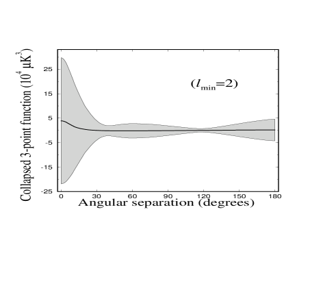
Figure 2 shows the collapsed three–point function $\bigl{\langle}C_{3}(\alpha)\bigr{\rangle}$ (solid line) and the grey band indicates the rms range of fluctuations expected from the cosmic variance. We have plotted the results for $x=0.07$, which looks as a reasonable value according to Ref. [23]. It is easy to find how these results change for other values of the parameter $x$, as the central curve $\langle C_{3}(\alpha)\rangle\propto x$, while the variance $\sigma_{CV}$ is approximately constant for small values of the $x$ parameter. The results do not include the dipole $(\ell_{min}=2)$, to match the COBE analysis. These results are to be compared with the data in Ref. [10]. For all reasonable values of the parameter $x$, the data falls well within the grey band, and thus there is good agreement with the observations. The cosmic variance band coming from the texture model is significantly larger than that coming from Gaussian distributed anisotropies [10, 15]. It is more than a factor 10 larger for angles smaller than $20^{\circ}$ and a factor 5 larger for larger angles. An increment in the cosmic variance has also been pointed out in Ref. [8] for the two–point correlation function, and has more extensively been studied in Ref. [30]. The fact that the range of expected values for the three–point correlation function predicted by inflation is included into that predicted by textures for all the angles and that the data points fall within them makes it impossible to draw conclusions favouring one of the models, although one may think that the fact that the data covers the full range of the band predicted by inflation means that the observed sky is a typical realization of the ensemble, while it is a less probable realization in the texture model as all the data fall close to the origin and the wide range of values allowed by the cosmic variance is nearly void.

The largest contribution to the cosmic variance comes from the small values of $\ell$. Thus, the situation may improve if one subtracts the lower order multipoles contribution, as in the $\ell_{min}=10$ analysis of Ref. [10].

  

FIG. 3.: Expected range of values for the three–point correlation function for the texture model with asymmetry parameter $x=0.4$ (grey band, as in Fig. 2). Also shown is the expected range for inflationary models (black band). Both bands include the $\sim 50\%$ increase in $\sigma_{CV}$ due to the sample variance. All multipoles up to $\ell=9$ have been subtracted. The right panel shows a zoomed fraction of the same plot.

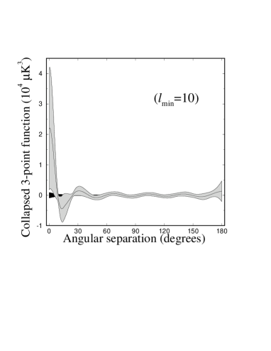
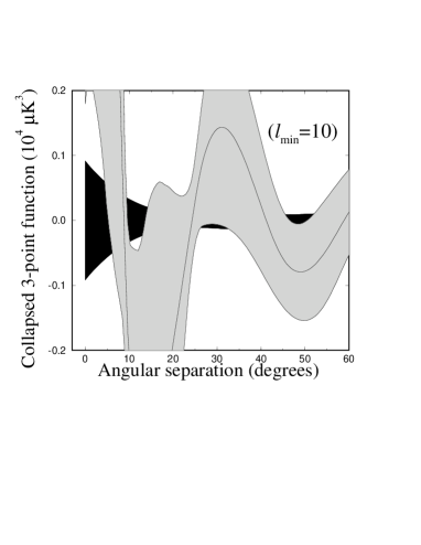
In Figures 3 a–b, we show by a grey band the expected range of values for the three–point correlation function for the texture model (as in Fig. 2) and by a black band the expected range for inflationary models. The bands do not superpose each other for some ranges of values of the separation angle for the value of $x=0.4$ considered, what means that measurements in that range can distinguish among the models. The value of the parameter $x$ considered is quite large, much in excess of that suggested by Ref. [23], but we have chosen it to show an example with a noticeable effect. We have checked that the non–superposition of the bands appears for $|x|>0.33$. The comparison with the data is less clear for this case, as the two–year COBE results have large instrumental noise (in excess of the Gaussian cosmic variance) for this subtraction scheme [10]. However, with the four–year data, the instrumental noise is expected to diminish under the cosmic variance, and it would be possible to distinguish among the models, at least for textures with $|x|>0.33$. On the other hand, already from the present data of Ref. [10] for small and very large angles, we can say that models with $x<-0.4$ are quite disfavoured.

An experiment probing smaller angular scales than COBE should thus be more appropriate to test non–Gaussian features in texture models. As an example we compute the predictions for a three–beam subtraction scheme experiment with window function at zero–lag ${\cal W}_{\ell}=(1.5-2P_{\ell}(\cos\theta)+0.5P_{\ell}(\cos 2\theta))^{1/2}\exp(-\ell(\ell+1)\sigma^{2}/2)$, where $\sigma=0.64^{\circ}$ is the beam width and $\theta=2.57^{\circ}$ is the chopping angle. This window function is peaked at $\ell\sim 70$ and the range of multipoles that significantly contribute to the three–point function is from $\ell=10$ to $\ell=100$. Hence we are still probing large enough scales and our results are not strongly affected by the microphysics of the last scattering surface, as it has recently been shown that the scale for the appearance of the so–called Doppler peaks within texture models is shifted to larger $\ell$’s than in the standard adiabatic case and their contribution turns out not to be dominant for this range of $\ell$’s [31, 32].

We obtain for the skewness $S\equiv\langle C_{3}(0)\rangle=(4.75\pm 1.94)\times 10^{4}\mu{\rm K}^{3}$, where the error band stands for the associated cosmic variance $\sigma_{CV}^{2}(0)$, for a value of the asymmetry parameter $x=0.07$. For comparison, the Gaussian adiabatic prediction is $S_{\rm Gauss}=0.06\times 10^{4}\mu{\rm K}^{3}$. Thus, in this case even for reasonably small values of the asymmetry parameter $x$ one such experiment can in principle distinguish between inflation and texture predictions, and thus put stronger constraints on the model parameters.

VI Discussion

We used an analytical model of the CMB anisotropies produced by textures to estimate the three–point correlation function and its cosmic variance. In spite of its simplicity, we expect that it can give a reasonable estimation of the results that would be obtained in numerical simulations. The idea of this analytical model [8] is that the texture evolution generates hot and cold spots in the sky at a constant rate per Hubble volume and Hubble time. Due to the scaling property of textures evolution the typical size of the spots is a constant fraction of the angle subtended by the Hubble radius at the time they are produced. The spot shapes are given by a profile function times a brightness factor. These free parameters have to be determined from the results of simulations. Here we have fixed the number density of spots produced per Hubble volume and Hubble time, the angular scale of the spots and the spots profile so that they are consistent with the results of Ref. [23]. The computations of the three–point function and the cosmic variance are fundamentally sensitive to the distribution of the spots brightness. A distribution symmetric in hot and cold spots gives rise to a vanishing three–point function, while a non–symmetric distribution yields a non–vanishing one. For definiteness, we parameterized the distribution with a very simple ansatz with just two free parameters, namely its dispersion, $\langle a^{2}\rangle$, and a parameter measuring the asymmetry of the distribution, $x$. $\langle a^{2}\rangle$ was fixed using the measured amplitude of the two–point correlation function. $x$ instead was left free and encodes the strongest dependence of our results on the model parameters. As discussed above, numerical simulations for random initial conditions point out to a non–vanishing asymmetry, although with a small value for $x$ (and large error bars). It is straightforward to extend the calculations to another brightness distribution.

The application of this analysis to the COBE–DMR experimental setting shows a very large cosmic variance band, much larger than that associated to a Gaussian process. For all reasonable values of $x$, this band encloses both the Gaussian one and the COBE data, and thus no conclusions favouring inflationary or texture theories can be obtained. The predictions of both models are consistent with the three–point function of the COBE–DMR maps. On the other hand when all the multipoles up to $\ell=9$ are subtracted, the situation looks a bit more promising and we saw that for large values of $|x|$, with the four years COBE data we could distinguish among texture and inflationary models. However, these large values of $x$ seem to be larger than those expected from simulations. Finally, we showed that a experiment probing smaller angular scales should be able to distinguish between both classes of models, even for small values of the modulus of the parameter $x$. This looks as an encouraging result in the task of testing theories of the primordial fluctuations.