A. Kogut^,3, A.J. Banday^2,4, C.L. Bennett⁵, K.M. Górski^2,6, G. Hinshaw²,

P.D. Jackson², P. Keegstra², C. Lineweaver⁷, G.F. Smoot⁷, L. Tenorio⁷, and E.L. Wright⁸

ABSTRACT

The Differential Microwave Radiometers (DMR) instrument aboard the Cosmic Background Explorer (COBE) has mapped the full microwave sky to mean sensitivity 26 ${\rm\mu K}$ per 7^∘ field of view. The absolute calibration is determined to 0.7% with drifts smaller than 0.2% per year. We have analyzed both the raw differential data and the pixelized sky maps for evidence of contaminating sources such as solar system foregrounds, instrumental susceptibilities, and artifacts from data recovery and processing. Most systematic effects couple only weakly to the sky maps. The largest uncertainties in the maps result from the instrument susceptibility to the Earth’s magnetic field, microwave emission from the Earth, and upper limits to potential effects at the spacecraft spin period. Systematic effects in the maps are small compared to either the noise or the celestial signal: the 95% confidence upper limit for the pixel-pixel rms from all identified systematics is less than 6 ${\rm\mu K}$ in the worst channel. A power spectrum analysis of the (A-B)/2 difference maps shows no evidence for additional undetected systematic effects.

Subject headings: cosmic microwave background – instrumentation: miscellaneous – artificial satellites, space probes

1 Introduction

The large angular scale anisotropy of the cosmic microwave background (CMB) reflects the distribution of matter and energy in the early Universe, before causal processes could operate to create the rich array of structures observed at the present epoch. Precise observations of the CMB anisotropy fix the initial conditions for different models of structure formation, and have important implications for theories of the high-energy behavior at the earliest times (e.g., inflation, cosmic defects). The Differential Microwave Radiometers instrument on the Cosmic Background Explorer (COBE-DMR) has completed its four-year observations of the microwave sky. It has detected statistically significant signals whose spatial morphology and frequency dependence are consistent with CMB anisotropy (Bennett et al. 1996, Bennett et al. 1994, Smoot et al. 1992). Microwave emission from the Galaxy is weak at high latitudes ($|b|{>}30{{}^{\circ}}$) and, with the notable exception of the quadrupole, does not significantly contaminate the primordial CMB signal (Kogut et al. 1996a, Kogut et al. 1996b, Bennett et al. 1992b). The CMB is isotropic to high degree: the detected anisotropy $\Delta T/T$ ranges from $10^{-6}$ to a few parts in $10^{-5}$ on angular scales larger than 7^∘. At this level of sensitivity, great care must be taken to demonstrate that the results are not affected by microwave emission from nearby objects hundreds to thousands of times hotter than the CMB (e.g., the spacecraft, Earth, Moon, and Sun) or from instrumental effects associated with changes in the orbital environment, telemetry, or data processing.

DMR is well characterized in terms of its response to various potential systematic effects. Kogut et al. (1992) describe the analysis techniques and upper limits on systematic artifacts in the first year sky maps. An important result of their analysis was that, owing to DMR’s rapid scan pattern and good pixel-pixel connectedness, most systematic effects couple only weakly to the sky maps. Non-celestial signals from nearby objects or within the instrument need not be removed to ${\rm\mu K}$ precision in the time domain for their effects in the map to be negligible. Bennett et al. (1994) provide similar analysis and upper limits for the two-year sky maps.

In this paper, we present the instrument calibration and upper limits to systematic artifacts in the final 4-year sky maps using data from 22 December 1989 through 21 December 1993 UT. Absolute calibration from external sources observed in flight (the Moon and the Doppler dipole from the Earth’s orbital motion about the Sun) are in agreement with the more precise pre-launch calibration; the calibration is determined to 0.7% absolute with drifts smaller than 0.2% per year. We detect gain modulation $\Delta{\cal G}/{\cal G}\approx 10^{-5}$ at the orbit period during the two-month periods surrounding the June solstice, when the spacecraft flies through the Earth’s shadow each orbit. The resulting modulation of the radiometric offset explains a previously detected instrumental signal of unknown origin during these periods.

The largest uncertainties in the maps result from the instrument susceptibility to the Earth’s magnetic field, microwave emission from the Earth, and upper limits to potential effects at the spacecraft spin period. We correct the data for the magnetic response; the resulting uncertainties are dominated by uncertainty in the magnetic field vector at each radiometer. With the full four-year data set we detect emission from the Earth when the Earth is 4^∘ below the Sun/Earth shields or higher (about 5% of the data); the detected signal is weak enough that correction is not required. There is no evidence for additional systematic effects at the spin period, but the precision with which we can rule out potential new effects is limited by the instrument noise. The quadrature sum of all systematic uncertainties in the 4-year maps, after correction in the time domain, yields upper limits $\Delta T{<}4~{}{{\rm\mu K}}$ rms over the full sky in the 4 most sensitive channels. Artifacts at this level would contribute less than 0.6% to the variance of the CMB signal at 7^∘ resolution: systematic effects do not limit the DMR maps.

2 Instrument Description

DMR consists of 6 differential microwave radiometers, 2 nearly independent channels (labeled A and B) at frequencies 31.5, 53, and 90 GHz (wavelength 9.5, 5.7, and 3.3 mm). Each radiometer measures the difference in power between two regions of sky separated by 60^∘, using a heterodyne receiver switched at 100 Hz between two corrugated horn antennas with beam width 7^∘ full width at half maximum pointed 30^∘ to either side of the spacecraft spin axis. The 31A and 31B channels share a common antenna pair in right and left circular polarizations; the other four channels have independent antenna pairs in a single linear polarization, for a total of ten antennas. The DMR antennas are mounted in 3 boxes spaced 120^∘ apart on the outside of the superfluid helium cryostat containing the Far Infrared Absolute Spectrophotometer (FIRAS) and the Diffuse Infrared Background Experiment (DIRBE). The E-plane of linear polarization in each of the 53 and 90 GHz antennas is directed radially outward from the spacecraft spin axis. A shield surrounds the aperture plane to block radiation from the Earth and Sun. The DMR antenna apertures lie approximately 6 cm below the shield plane. The combined motions of the spacecraft spin (75 s period), orbit (103 m period), and orbital precession ($\sim 1{{}^{\circ}}$ per day) allow each sky position to be compared to all others through a highly redundant set of all possible difference measurements spaced 60^∘ apart.

The switched signal in each channel undergoes RF amplification, detection, near-dc amplification, and synchronous demodulation. The demodulated signal is integrated for 0.5 s, digitized, and stored in an on-board tape recorder. A single local oscillator provides a common frequency reference for the mixer in the A and B channels at each frequency. The A and B channels also share a common enclosure and thermal regulation system but are otherwise independent. We also sample the switched signal after one stage of dc amplification but before synchronous demodulation; the resulting “total power” signal serves as a low-precision check on the system temperature and gain of the RF and first dc amplifier with only minor contributions from celestial signals.

COBE was launched from Vandenberg Air Force Base on 18 November 1989 into a 900 km, 99^∘ inclination circular orbit which precesses to follow the terminator. Attitude control keeps the spacecraft pointed away from the Earth and nearly perpendicular to the Sun. Solar radiation never directly illuminates the aperture plane. The Earth limb is below the shield for 95% of the mission. During the 2 months surrounding the June solstice, the attitude control can not simultaneously block both terrestrial and solar emission, and the Earth limb rises above the shield as the spacecraft flies over the Arctic. During the same 2 months, the spacecraft flies through the Earth’s shadow over the Antarctic. The resulting eclipse modulates spacecraft temperatures and voltages.

Several authors provide a more complete description of COBE and DMR. Boggess et al. 1992 provide a mission overview. Smoot et al. 1990 describe the DMR instrument. Toral et al. 1990 and Wright et al. 1994 describe the DMR beam patterns. Bennett et al. 1992a describe the instrument pre-flight calibration and provide a schematic of the COBE aperture plane.

3 Data Processing

The digitized data from the on-board tape recorders are transmitted once per day to a ground station. A software program merges the uncalibrated DMR differential data with housekeeping (temperatures, currents, voltages, and relay states), spacecraft attitude, and selected spacecraft archives (magnetometers, momentum wheels, electromagnet currents). The uncalibrated time-ordered data $S_{ij}(t)$ may be represented as

$$S_{ij}(t)=\frac{1}{{\cal G}(t)}~{}[~{}T_{i}-T_{j}~{}+~{}O(t)~{}+~{}N(t)~{}+~{}\sum_{k}Z_{k}(t)~{}]$$

where $T_{i}$ and $T_{j}$ are the antenna temperatures of the two regions of sky observed at time $t$, ${\cal G}(t)$ is the gain factor providing calibration between antenna temperature and telemetry units, $O(t)$ is the radiometric offset produced by small imbalances in the differential radiometer, $N(t)$ is the random instrument noise, and $Z_{k}(t)$ are the time-dependent systematic signals from non-cosmological sources and instrumental effects. A second program calculates the gain factor ${\cal G}^{\prime}(t)$, the instrumental baseline $B(t)$, and corrections for known systematics $W_{n}(t)$ to determine the calibrated differential temperatures

$$D_{ij}(t)={\cal G}^{\prime}(t)[S_{ij}(t)~{}-~{}B(t)]~{}-~{}\sum_{n}W_{n}(t)$$

which we refer to as the DMR time-ordered data set.

The instrument gain, beam patterns, and environmental susceptibilities of each radiometer have been measured in pre-flight testing (Smoot et al. 1990). Based on these and on in-flight data, we reject data taken when the uncertainty in the systematic error model $W_{n}(t)$ becomes unacceptably large. Table 1 lists cuts and corrections made in the 4-year DMR data processing. We flag as unusable any datum for which the telemetry is unavailable or of poor quality, or which deviates from the mean by more than 5 standard deviations. Such “spikes” are rarely noise outliers, but result instead from observations of the Moon or instrument changes such as the end of the noise source calibration sequence. The exponential decay of the noise source power contaminates the first few samples after the noise sources have been commanded off; as a result, we conservatively discard the entire 32 s frame after each in-flight calibration.

We flag as unusable for sky maps any datum taken with the Moon within 21^∘ of an antenna beam center, although we do use these data for lunar calibration and to map the beam pattern in flight. All other data are corrected for a model of lunar emission. We reject data taken when the Earth limb is 1^∘ below the shield or higher (3^∘ for the 31.5 GHz channels) but do not otherwise correct for Earth emission. We correct data taken with Mars, Jupiter, or Saturn within 15^∘ of an antenna beam center but do not reject these data as unusable. We correct the time-ordered data for the instrument response to the Earth’s magnetic field, the 3.2% correlation between successive observations caused by the lock-in amplifier low-pass filter, and for the Doppler dipole from the satellite motion about the Earth and the Earth’s orbital motion about the solar system barycenter. An orbitally-modulated signal is present during the 2-month “eclipse season” surrounding the June solstice, related to thermally-induced gain variations in the amplification chain. An empirical model based on tracers with high signal to noise ratio removes approximately 2/3 of this signal. Estimated residuals, after correction, are small compared to the increase in data and sky coverage in the 53 and 90 GHz channels (recall that orbitally modulated signals couple only weakly to the sky maps, so that a small systematic signal accompanied by a larger increase in sensitivity can be a worthwhile trade-off). The amplitude of the effect, and hence the residual uncertainty, is larger in the 31A and 31B channels; we reject data taken during the period May 1 through August 4 of each year for the 31A channel and May 21 through July 24 for the 31B channel. The 31B channel suffered a permanent increase in receiver noise on 4 October 1991. We flag as unusable data when the instrument noise is unstable, and use the noise during stable periods to weight all analyses. As a result, the 31B results are approximately 30% noisier than the 31A channel.

We fit the time-ordered data to a pixelized sky map and systematic terms by minimizing the $\chi^{2}$ sum

$$\chi^{2}=\sum_{t}~{}[~{}\frac{D_{ij}(t)~{}-~{}(T_{i}-T_{j})}{\sigma_{ij}(t)}~{}]^{2}$$ (1)

where $\sigma_{ij}(t)$ is the instrument noise (Bennett et al. 1996). A sparse-matrix algorithm performs the inversion and yields a set of pixel temperatures $T_{i}$ and coupling coefficients $a_{n}$ to specified systematic effects (Janssen & Gulkis 1992, Jackson et al. 1992, Torres et al. 1989).

Several methods exist to derive limits to systematic signals $Z_{k}(t)$ in the time-ordered data and their projection $\Delta T_{\rm sys}$ in the sky maps. Given a time-dependent model $W_{n}(t)$, a linear least-squares method solves simultaneously for the systematic coupling coefficient $a_{n}$ in the time domain and the sky temperatures $T_{i}$ in the map (Eq. 1). This procedure automatically removes the best estimate of the particular systematic signal from the sky map. We make a map $\Delta T_{\rm sys}$ of the removed systematic effect by subtracting two solutions to Eq. 1 which differ only in the presence or absence of the model function $W_{n}(t)$. The residual uncertainty $\delta T_{\rm sys}$ after correction is determined by multiplying the systematic map $\Delta T_{\rm sys}$ by the fractional uncertainty in the coupling coefficient:

$$\delta T_{\rm sys}=\frac{\delta a_{n}}{a_{n}}\Delta T_{\rm sys}.$$ (2)

In some cases, the model function $W_{n}(t)$ may not be well specified a priori. We may re-bin the time-ordered data into a coordinate system where the signal will add coherently to obtain limits to both the shape and amplitude of the systematic function $Z_{k}(t)$. We then use the binned data and associated uncertainties, sampled according to the DMR observation pattern, as the model function $W_{n}(t)$ in Eq. 1 to derive the systematic error map and uncertainty. For example, microwave emission from the Earth diffracted over the shield has a complicated time dependence whose exact form depends sensitively upon the relative geometry of the Earth, shield, and horn antennas. We bin the data by the location of the Earth relative to the COBE aperture plane and use the binned data both to evaluate various models $W_{n}$ of the diffraction and to derive model-independent limits to Earth emission in the DMR maps. We also bin the time-ordered data by the spacecraft orbit and spin angles to search for signals at those periods.

Several tests limit systematic effects without requiring any a priori information. Fourier transforms of the calibrated $D_{ij}(t)$ provide a powerful tool to limit potential effects. Common-mode signals, particularly celestial emission, cancel in the (A-B)/2 “difference map” linear combination of the A and B channels at each frequency, or in similar difference maps from different time ranges in a single channel. Analysis of the difference maps provides model-independent limits to the combined effects of all systematic effects which are not identical in different channels or at different times.

The instrument noise is well described by a Gaussian probability distribution with standard deviation depending on the number of discrete observations $N_{i}$ per pixel,

$$n_{i}=\frac{\sigma_{0}}{\sqrt{N_{i}}},$$

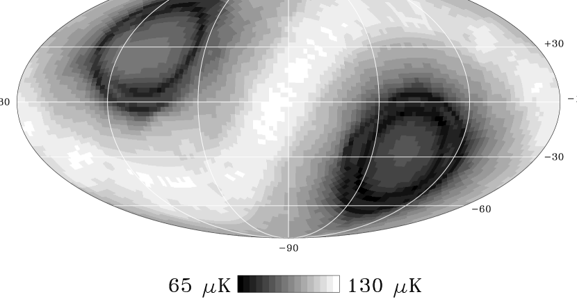
Figure 2: Noise pattern of the 53B channel for 4 years of data. The map is a Mollweide projection in Galactic coordinates. The lunar cut causes the striping in the ecliptic plane, while the cut for the Earth limb causes the north-south asymmetry near the ecliptic poles.

where $\sigma_{o}$ is the rms noise per 0.5 s observation (Bennett et al. 1996). Figure 1 shows the instrument noise sorted by the number of observations linking two pixels at 60^∘ separation. There is no evidence for a “noise floor” from effects which do not average out with time. Figure 2 shows the observation pattern in the 53B channel for the 4-year mission after applying all cuts. Correlations between pixels caused by the 60^∘ antenna separation are negligible (Lineweaver et al. 1994). Because COBE is in a polar orbit, regions approximately 30^∘ from the celestial poles are observed each orbit, while regions near the celestial equator are only observed for 4 months of each year. The lunar cut further reduces usable data near the ecliptic plane. Since the model functions $W_{n}(t)$ are typically not well described by a set of temperatures $T_{i}$ fixed on the sky, gradients in the sky coverage are apparent in many of the systematic error maps.

4 Calibration

The primary DMR calibration consists of the radiometric comparison, before launch, of cold ($\sim$77 K) and warm ($\sim$300 K) full-aperture blackbody targets. In addition, noise sources inject $\sim$2 K of broad-band power into the front end of each radiometer between the horn antenna and the Dicke switch. Near-simultaneous observations of the blackbody targets and the noise sources calibrate the antenna temperature of each noise source and permit the transfer of the blackbody calibration standard to the flight observations (Bennett et al. 1992a). Observations of the Moon and CMB dipole provide additional in-flight calibration. Table 2 summarizes the DMR calibration over the 4-year mission.

4.1 Absolute Calibration

The pre-flight absolute calibration has been adjusted for two effects observed in the first year of the mission: the 31B gain was decreased by 4.9% and the 90B gain increased by 1.4% (Kogut et al. 1992). Errors in the absolute calibration create systematic artifacts in two ways: errors in the amplitude of detected structures in the sky, and artifacts in maps from which a model of celestial emission (e.g., lunar emission) have been removed. Observations of the Doppler dipole from the Earth’s orbital velocity provide an independent absolute calibration in flight. Motion with velocity ${\bf\beta}$ through an isotropic blackbody radiation field at temperature $T_{0}$ creates an observed thermodynamic temperature distribution

$$T(\theta)=\frac{T_{0}(1-\beta^{2})^{1/2}}{1-\beta\cos(\theta)}\approx T_{0}[1+\beta\cos(\theta)+O(\beta^{2})]$$ (3)

(Peebles & Wilkinson 1968). The CMB spectrum is well described by a blackbody with $T_{0}$ = 2.728 K (Fixsen et al. 1996). The dipole caused by the Earth’s orbital velocity about the solar system barycenter (29.27 km s^-1 to 30.27 km s^-1) provides a calibration signal $\Delta T\approx 270$ ${\rm\mu K}$ whose known spatial and temporal dependence allows simple separation from other astrophysical signals. Figure 3 shows the modulation of the CMB dipole observed in the 53B channel throughout the 4-year DMR mission. We fit the time-ordered data for a fixed sky map plus a Doppler calibration term, including the change in the orbital speed from the eccentricity of the Earth’s orbit. Table 3 compares the Doppler calibration to the primary calibration. Values larger than unity indicate a channel in which the observed Doppler dipole is larger than predicted. The Doppler calibration is in agreement with the more precise pre-launch absolute calibration and shows no evidence for calibration shifts at the few percent level.

If we accept the pre-launch calibration as accurate, the Earth Doppler dipole provides a determination of the absolute CMB temperature $T_{0}$. We may use Eq. 3 and the Doppler calibration factors from Table 3 to infer the CMB absolute temperature: $T_{0}~{}=2.83\pm 0.07$ K at 31.5 GHz, $2.71\pm 0.03$ K at 53 GHz, and $2.72\pm 0.04$ K at 90 GHz for a weighted mean $T_{0}=2.725\pm 0.020$ K (68% CL), in excellent agreement with the FIRAS spectrum.

Figure 4 shows the Doppler dipole resulting from COBE’s 7.5 km s^-1 orbital velocity about the Earth. We have mapped the time-ordered data in a coordinate system co-moving with the satellite velocity vector, and binned the resulting map temperatures by the angle from the velocity vector. The attitude control system prevents DMR from observing all angles in this coordinate system. Within the range of angles observed, we find good agreement with the predicted 70 ${\rm\mu K}$ dipole. The COBE velocity dipole demonstrates the sensitivity to signals $\Delta T/T\sim 10^{-5}$.

The Moon provides a second external absolute calibration source. DMR observes the Moon in the antenna main beam for $\sim$6 days each at both first and third quarters (Bennett et al. 1992a). The antenna temperature of the Moon within integration time $\tau$ is given by

$$T_{A,{\rm Moon}}~{}=~{}\frac{1}{\tau}~{}\int^{t+\tau}_{t}dt~{}\int d\Omega~{}T_{\rm Moon}~{}P[\theta(t),\phi(t)]~{}/~{}\int d\Omega~{}P(\theta,\phi)$$

where $P(\theta,\phi)$ is the DMR beam pattern. We integrate the physical temperature and microwave emission properties across the lunar disk to estimate $T_{\rm Moon}$ as a function of lunar phase and Sun-Moon distance (Keihm 1982, Keihm & Gary 1979, Keihm & Langseth 1975). The gain factors derived from observations of the Moon show a pronounced dependence on lunar phase, with peak-to-peak variation of 3.7%, 5.3%, and 6.2% at 31.5, 53, and 90 GHz, respectively. Longer term analysis shows an additional annual modulation with peak-to-peak amplitude 2%. These apparent gain modulations are not present in any method which does not involve lunar observations (i.e., on-board noise sources or the CMB dipole). We thus ascribe them to real time-dependent effects in $T_{\rm Moon}$ which are not duplicated in the Keihm model. See Jackson et al. 1996 for further analysis of $T_{\rm Moon}$.

The lunar calibration modulation is repeatable over the 4-year mission and may be removed empirically to provide a stable “standard candle” for relative gain analysis. We adopt the combined peak-peak modulation as an estimate of the uncertainty of the lunar model for the absolute calibration. Table 3 shows the mean lunar calibration compared to the noise source calibration. The channel averaged lunar absolute calibration is 1.8% larger than the pre-launch absolute calibration, well within the systematic limitations of the lunar model.

The Moon also serves to cross-calibrate the A and B channels. Systematic uncertainties in the model for $T_{A,{\rm Moon}}$ cancel in the A/B ratio at each frequency. The resulting ratio (Table 4) places a limit to how well celestial emission will be expected to cancel in the (A-B)/2 “difference maps.” A similar analysis for the Earth velocity Doppler effect is consistent within much larger uncertainties. The A and B channels are cross-calibrated within 0.4%, well within the accuracy of the pre-flight calibration.

4.2 Relative Calibration

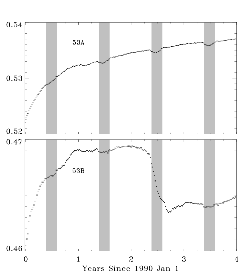
Figure 5: Calibration factor ${\cal G}^{\prime}(t)$ derived from on-board noise sources for the 53A and 53B channels. Each datum represents one week. The gray bands show the “eclipse season” surrounding the June solstice. The gain is stable to better than 3% throughout the 4-year mission.

The noise sources are commanded on for 128 seconds every two hours. Provided the power broadcast by each device is constant in time, they provide a standard to monitor time-dependent changes in the instrument calibration. Figure 5 shows the calibration ${\cal G}^{\prime}(t)$ derived from the noise sources for the 53A and 53B channels over the full 4-year mission. The gain is stable to better than 3% throughout the 4-year mission. Gain drifts per se do not create systematic artifacts provided the noise sources track the true calibration ${\cal G}(t)$.

Each noise source is observed in both the A and B channels. The ratio of the two noise sources in a single channel provides information on the noise source stability, since the instrument calibration cancels. The ratio of a single noise source observed in two channels provides information on gain stability, since the noise source performance cancels. Based on these ratios, we correct the data for 3 step changes in noise source broadcast power: a 0.69% increase in power for the 90 GHz “down” noise source on 17 March 1990, a 0.69% increase in power for the 31 GHz “down” noise source on 11 February 1992, and a 0.34% increase in power for the 90 GHz “down” noise source on 26 November 1993. An additional anomaly occurred on 1 September 1993 in the 90 GHz data, when both noise sources showed step changes in a pattern inconsistent with a simple change in power or instrument calibration. A 0.29% step increase occurred for the 90A channel “up” noise source which was not mirrored by the same noise source observed in the 90B channel. At the same time, the “down” noise source in the 90B channel decreased in power by 0.66%, unaccompanied by a similar change in the 90A channel. Since a calibration change would show up as a step in both the “up” and “down” noise source signals, while a noise source power change would show up in both the 90A and 90B channels, we can rule out simple models involving a single component. We currently have no explanation for this event, but remove its effects in software by increasing the “up” noise source by 0.29% for the 90A channel only and decreasing the “down” noise source by 0.66% for the 90B channel only.

4.2.1 Long-Term Calibration Drifts

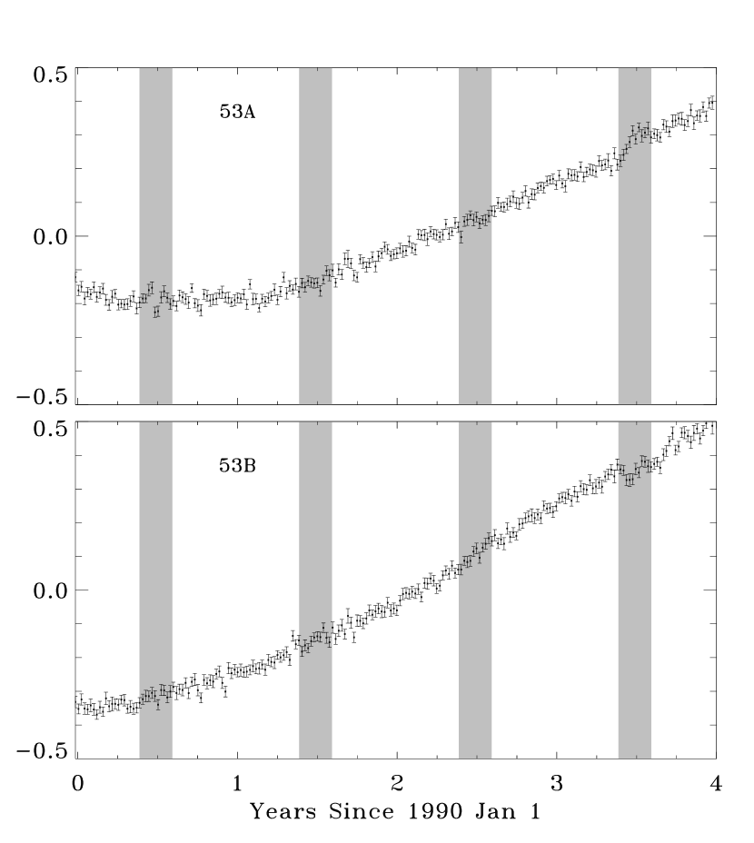
Figure 6: Ratio of “up” and “down” noise sources vs time for 53A and 53B channels. Each datum represents one week. The gray bands show the “eclipse season” surrounding the June solstice. Uncorrected linear drifts are smaller than 0.2% per year at 95% confidence.

The gain solutions in the 90A and 90B channels are corrected for linear drifts of 0.81% yr^-1 and 0.87% yr^-1 respectively (Kogut et al. 1992, Bennett et al. 1994). We place limits on un-corrected long-term drifts in noise source power by examining the ratio of the A and B noise sources in each channel. The instrument calibration cancels in this ratio, which places a lower limit to the long-term accuracy of the calibration solution (which assumes that the noise sources do not change in time). Figure 6 shows this ratio for both the 53A and 53B channels. Channel 53A shows a stable ratio for the first year followed by a linear drift, while channel 53B shows an approximately linear drift throughout the mission. The fact that the ratio of the same physical devices does not have the same shape in both channels indicates that the observed changes are caused by a process more complicated than a simple change in noise source broadcast power. Table 5 shows the limits to linear drifts in all 6 channels based on the noise source ratios.

The CMB dipole provides a continuously observed signal of 3 mK amplitude, which we use to limit long-term errors in the noise source calibration. We fit the time-ordered data to the form

$$\Delta T~{}=~{}(1+bt)~{}\sum_{\ell=1}^{2}\sum_{m=-\ell}^{\ell}~{}a_{\ell m}Y_{\ell m},$$

i.e., a spatially fixed dipole and quadrupole whose amplitudes change linearly with time. Since the CMB is effectively a constant for the four years of DMR observations, we can interpret the fitted parameter $b$ in terms of a linear drift in the true calibration ${\cal G}(t)$ relative to the noise source solution ${\cal G}^{\prime}(t)$. Table 5 shows the resulting limits to calibration drifts. There are no drifts significant at 95% confidence level.

The Moon also serves as a standard candle once the annual and phase variations are empirically removed. We have analyzed the ratio of the corrected lunar calibration to the noise source calibration to search for long-term drifts in the noise source solution (Table 5). The drifts inferred from the noise sources, dipole, and Moon are in general agreement and provide some evidence that calibration drifts are dominated by changes in the power emitted by the noise sources. The significance of the coefficients is difficult to evaluate. The uncertainties in Table 5 are statistical only. Since the lunar results are possibly affected by long-term artifacts related to the annual and phase variations, and since the noise source ratios are clearly more complicated than a simple linear drift, we do not use a weighted estimate of the three techniques. Instead, we adopt the unweighted mean and use the scatter among the three techniques as an estimate of the uncertainty. Table 2 shows the resulting limits on long-term calibration drifts in the 4-year DMR data set.

4.2.2 Orbital Calibration Drifts

The noise sources provide direct calibration information every two hours. We interpolate the noise source gain solution ${\cal G}^{\prime}(t)$ using 48 hours of data fitted to a cubic spline with one interior knot. The resulting gain solutions are smooth at the daily boundaries but can not respond to gain variations with periods shorter than about 8 hours. We estimate gain variations at the orbit period by fitting a long-term baseline to the noise source calibrations and binning the residuals by the spacecraft orbit angle relative to the ascending node. Long-term plots of the calibration (Fig. 5) show effects related to the “eclipse season” surrounding the June solstice. Figure 7 shows the binned calibration residuals during eclipse season and for “non-eclipse” data (the rest of each year). The noise sources (top panels) show gain variation with amplitude $\Delta{\cal G}/{\cal G}~{}\approx~{}1.6\times 10^{-4}$ during the eclipse season. The shape of the gain variation is nearly identical to the spacecraft temperature variations, here (superimposed solid line) represented by a thermistor in the Instrument Power Distribution Unit (IPDU). Since the IPDU is not thermally controlled, it shows larger temperature variations which are less affected by the housekeeping digitization. The total power (middle panels), binned in a similar fashion, shows similar modulation, supporting the existence of a real orbitally-modulated gain variation during the eclipse season. The amplitude of the total power variation, $\Delta P/P~{}\approx~{}6.1\times 10^{-5}$, is smaller than the noise source variation, as expected since the total power does not sample the entire amplification chain.

The mixer/preamp assembly and lock-in amplifier are maintained in a thermally controlled box. Figure 7 also shows the lock-in amplifier temperature (bottom panels) during eclipse and non-eclipse data. Thermal variations of $\sim$10 mK amplitude at the orbit period are observed during eclipse season, compared to $\sim$6 K for the unregulated IPDU. The thermal susceptibility of the amplifiers, measured prior to launch, is $\Delta{\cal G}/{\cal G}\approx 1\%~{}{\rm K}^{-1}$ (Bennett et al. 1992a). The observed orbital gain variations are consistent with thermal modulation at the 10 mK level.

The existence of gain modulation $\Delta{\cal G}/{\cal G}\approx 10^{-4}$ with wave form similar to the IPDU thermistor provides a plausible explanation for a previously detected signal during eclipse season (§5.2; see also Kogut et al. 1992 and Bennett et al. 1994). An empirical fit to the IPDU thermistor and voltage monitors removes most of this signal; we do not explicitly correct the noise source solutions to model the orbital gain variation during eclipse season. Outside of eclipse season, the orbital environment is stable. The amplifier temperatures and direct noise source calibration show no modulation at the orbit period. The total power shows slight orbital modulation linked to variations in the input celestial signal from the CMB dipole and Galactic plane. There is no evidence for orbitally modulated gain variation outside of the eclipse season at the level of a few parts in $10^{5}$ (Table 2, column 6).

The noise source calibrations require 128 s, longer than the 73 s spin period. We obtain limits on calibration modulation at the spin period by binning the total power signal (sampled every 8 s) and scaling the resulting limits using the ratio of total power to gain variations observed at the orbit period, $\Delta{\cal G}/{\cal G}=3.1\Delta P/P$. We find no variation in either the total power or the amplifier temperature at the spin period (Table 2, column 7), with limits $\Delta{\cal G}/{\cal G}~{}{<}~{}2\times 10^{-6}$ (95% CL).

Gain modulation can create systematic artifacts in two ways: through observations of the sky at different relative calibration (“striping”), and by modulating the radiometric offset. The relative importance of the two effects depends on the time scale. Over long periods, the offset signal $\Delta{\cal G}/{\cal G}\times O(t)$ is removed by the fitted baseline, leaving striping as the primary gain artifact. On time scales comparable to the spin or orbit periods, offset modulation becomes dominant. Since the offsets can approach 1 K, a gain modulation as small as $10^{-4}$ can create a 100 ${\rm\mu K}$ signal. We derive upper limits on the systematic artifacts in the DMR sky maps resulting from calibration drifts at the spin, orbit, or longer periods by adding terms to Eq. 1 of the form $W_{n}=\Delta{\cal G}(S_{ij}(t)+B(t))$ where $\Delta{\cal G}(t)$ is taken from the 95% confidence upper limits in Table 2. That is, we simulate the effect of an uncorrected calibration modulation in the striping of the sky, the modulation of the instrumental offset, and possible cross-talk with other systematic effects. Systematic artifacts from residual calibration drifts and modulation are negligible, creating rms variations 0.4 ${\rm\mu K}$ or smaller (95% CL) in the most sensitive sky maps.

5 Environmental Effects

The COBE orbit provides a generally benign environment for the DMR instrument. The radiometers are above the Earth’s atmosphere, and the terminator-following orbit prevents large temperature changes. Kogut et al. (1992) review various effects associated with the orbital environment. The largest signals result from the response of the Dicke switch to the Earth’s magnetic field, and the thermal response of the amplifiers to temperature changes when the orbit passes into the Earth’s shadow. We correct for both of these effects; residual artifacts in the sky maps are small.

5.1 Magnetic Susceptibility

The amplification chain in each channel is connected to the antennas using a latching ferrite circulator switched at 100 Hz by an applied magnetic field. An external magnetic field (from the Earth or the electromagnets used to control the spacecraft angular momentum) modulates the insertion loss of the switch and creates a time-dependent signal described by the vector coupling

$$Z_{\rm magnetic}(t)=\vec{\beta}~{}\cdot~{}\vec{B}(t)$$ (4)

where $\vec{B}(t)$ is the magnetic field vector. We express the magnetic susceptibility vector $\vec{\beta}$ in an orthonormal coordinate system fixed with respect to the spacecraft: $\beta_{X}$ is the susceptibility along the X axis (antiparallel to the spin axis), $\beta_{R}$ is the susceptibility along the radial axis (directed outward between two antennas), and $\beta_{T}$ is the susceptibility along the transverse axis (from the positive horn to the negative horn). The antennas are pointed 30^∘ to either side of the $X$ axis; magnetic signals from the $\beta_{X}$ susceptibility are not spin modulated and produce a signal at the orbit period only. Both the $R$ and $T$ signals are spin modulated. The $\beta_{R}$ susceptibility produces an apparent temperature gradient oriented across the magnetic field (east-west) but at right angles to the antenna pointing. The $\beta_{T}$ susceptibility produces an apparent temperature gradient oriented along the magnetic field (north-south) in phase with the antenna pointing. The inclination of the COBE orbit with respect to the magnetic poles breaks the degeneracy which would otherwise make the $\beta_{T}$ susceptibility indistinguishable from a celestial dipole aligned with the Earth’s magnetic field.

Figure 8 shows the model magnetic signal $Z_{\rm magnetic}(t)$ for for the 53B radiometer over the course of several orbits. The spacecraft spin modulates both the radial and transverse field components, causing the rapid variation at the spin period. The spacecraft orbital motion samples the Earth’s field at different latitudes, causing an orbital drift and modulating the amplitude envelope of the spin variations. The resulting signal is quite distinct from that expected from a fixed celestial signal, represented in Figure 8 by a model of lunar emission. The different time-dependent signatures greatly reduce the required accuracy of the magnetic model.

We simultaneously fit the time-ordered data in each channel for the temperature in each pixel and the magnetic susceptibility vector $\vec{\beta}$ (Eqs. 1 and 4). We obtain a significant improvement in $\chi^{2}$ in each channel, demonstrating that the DMR magnetic signals are not well described by any set of fixed pixel temperatures. More complicated models of the magnetic coupling (e.g., tensor or non-linear terms) do not further reduce the $\chi^{2}$: a linear vector model (Eq. 4) is sufficient. We also fit $\vec{\beta}$ independently to each month of data and search for time dependence in the fitted coefficients. If the data are not corrected for the eclipse-related effects, all channels show anomalies in the $\beta_{X}$ coefficients during the eclipse season. After correcting the time-ordered data for this effect (§5.2), the 31A and 31B channels show additional modulation of the $\beta_{X}$ susceptibilities with a period of one year. We modify Eq. 4 to include additional terms of the form $\beta_{\rm annual}\cos\theta\cos\phi$ where $\theta$ is the orbit angle relative to the ascending node and $\phi$ is the angle of the orbit plane relative to the vernal equinox. Since the resulting signal is not spin-modulated, it has almost no effect on the sky maps but is included to reduce cross-talk with other orbitally modulated effects. The 53 and 90 GHz channels show no significant variation in the fitted magnetic coefficients.

Table 6 lists the magnetic coefficients derived from 4 years of data. Slow changes in the magnetic signal from the orbitally-modulated $\beta_{X}$ susceptibility may be removed as part of the baseline. The values in Table 6 refer to the two-orbit running mean baseline (Bennett et al. 1994) for which no such subtraction takes place.

We model the magnetic field $\vec{B}(t)$ using the spacecraft attitude solution and the time-dependent 1985 International Geomagnetic Reference Field (Barker et al. 1986) to order $\ell=8$. We neglect the field components at higher $\ell$ and any contribution from the electromagnets used to dissipate spacecraft angular momentum. The amplitude of the field model varies from 196 to 402 mG over the COBE orbit. We limit deviations from the true field and our field model by using on-board magnetometers and find good agreement between the magnetometers and our application of the field model. We have examined the residuals for coherent behavior with respect to an inertial coordinate system (e.g., if the electromagnets preferentially fired with the spacecraft in a fixed location and attitude) and find none. The rms difference between the magnetometers and the field model is 8.9 mG averaged over the 4-year mission, which we adopt as the 68% CL uncertainty in the application of the model.

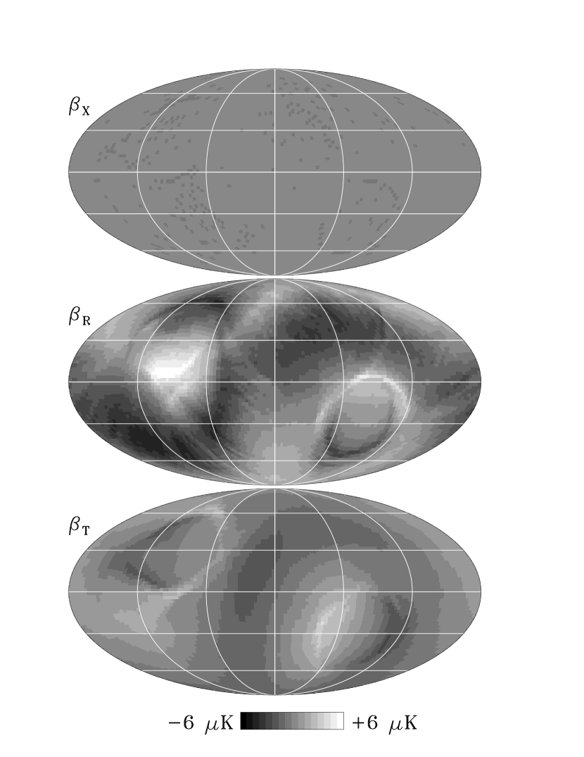
Figure 9: Full sky maps of 95% CL upper limits to the residual effect, after correction, of the magnetic susceptibility in the 53B channel. The maps are Mollweide projections in Galactic coordinates. (top) $\beta_{X}$ susceptibility. (middle) $\beta_{R}$ susceptibility. (bottom) $\beta_{T}$ susceptibility. A fitted dipole has been removed from each map to show the higher-order structure.

The simultaneous fit for the pixel temperatures and magnetic coefficients removes the fitted magnetic signals from the sky maps. The uncertainties in the fitted coefficients are dominated either by instrument noise (if $\vec{\beta}{{}_{<}\atop{}^{\sim}}0.3~{}{\rm mK~{}G}^{-1}$) or by the uncertainty in the magnetic field model. We obtain a map of the removed signal by subtracting the corrected sky map from a similar map for which no magnetic terms were fitted. We estimate the residual uncertainties after correction by multiplying this “effect” map by the fractional uncertainty in each fitted coefficient (Eq. 2). Figure 9 shows the 95% CL uncertainties in the 53B channel from magnetic effects. The magnetic residuals are among the largest systematic uncertainties in the DMR sky maps, but the amplitudes are small: the residual magnetic uncertainty, after correction, is less than 3 ${\rm\mu K}$ rms in any channel.

5.2 Seasonal Effects

Previous analysis of the 1- and 2-year data sets showed the presence of an orbitally modulated signal during the “eclipse season” surrounding the June solstice when the spacecraft repeatedly flies through the Earth’s shadow (Kogut et al. 1992, Bennett et al. 1994). This “eclipse effect” is strongly correlated with various housekeeping signals, particularly the unregulated spacecraft temperatures and bus voltages which show the largest variation during eclipses and are thus least affected by the telemetry digitization (see Figure 4 of Kogut et al. 1992) We model the effect empirically by fitting the time-ordered data to the form

$$Z_{\rm eclipse}~{}=~{}a~{}\Delta T_{\rm IPDU}~{}+~{}b~{}\Delta V_{\rm 28}$$

where $\Delta T_{\rm IPDU}$ is the temperature of the IPDU box and $\Delta V_{\rm 28}$ is the 28V bus voltage. We remove an orbital mean from both $\Delta T_{\rm IPDU}$ and $\Delta V_{\rm 28U}$ prior to fitting since long-term drifts are removed as part of the instrument baseline. The resulting peak-peak changes in the housekeeping signals are $\Delta T_{\rm IPDU}~{}\sim$ 5.3 du, $\Delta V_{\rm 28}~{}\sim$ 4.3 du during eclipse season, and $\Delta T_{\rm IPDU}~{}\sim$ 0.3 du, $\Delta V_{\rm 28}~{}\sim$ 0.1 du excluding eclipse season, where the housekeeping signals are expressed in digitized telemetry units (du). Table 7 shows the fitted coefficients for this empirical model during and excluding eclipse season. We detect the effect in all channels during eclipse season. Outside of eclipse season, the spacecraft temperatures and voltages are stable and the effect vanishes.

The detection of thermal gain variations at the orbit period during eclipse season (§4.2.2) provides a plausible mechanism for the eclipse effect. However, neither the observed gain variations nor the empirical housekeeping correlations remove the entire eclipse signal in all channels. The magnetic $\beta_{X}$ coefficients for the 31A and 31B channels remain anomalously large during eclipse season even after correction for $Z_{\rm eclipse}$, indicating that the empirical model removes only 2/3 of the signal in those channels. The eclipse effect creates artifacts in the maps in two ways: the direct projection of the signal into the maps, and cross-talk with other orbitally modulated effects (particularly the $\beta_{X}$ magnetic susceptibility). Both effects are important for the 31A and 31B channels; accordingly, we do not use data during eclipse season for these channels. The 53 and 90 GHz channels have smaller eclipse coefficients and show no $\beta_{X}$ anomalies after correction. We correct the data using the empirical model and estimate the residual uncertainties in the sky maps using Eq. 2. Since the eclipse signal does not vary at the spin period, its projection onto the maps is small. Including the eclipse data in the 53 and 90 GHz channels adds less than 0.3 ${\rm\mu K}$ rms artifacts to the maps (95% CL), much less than the 10 ${\rm\mu K}$ reduction in noise gained by adding the 8 months of eclipse data to the 4-year data set.

5.3 Orbit and Spin Effects

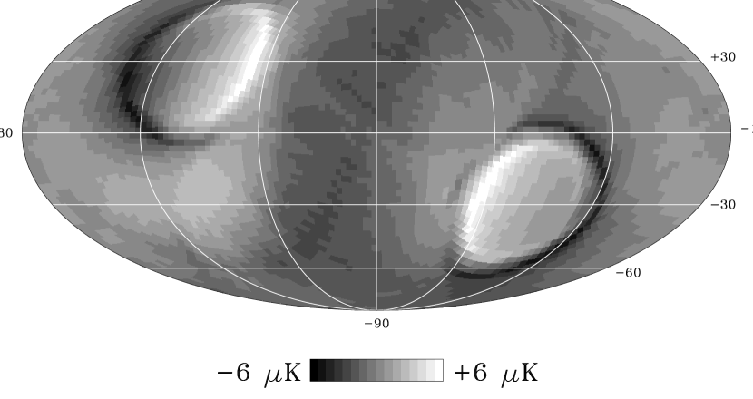
Figure 10: Full sky map of 95% CL upper limits to spin-modulated effects in the 53B channel (Mollweide projection in Galactic coordinates). A fitted dipole has been removed to show the higher-order structure. The amplitude of the structure in this map is dominated by the instrument noise binned at the spin period.

The spacecraft orbit and spin provide a natural period for any environmental effects. We test for the presence of additional effects, independent of an a priori model, by binning the corrected data $D_{ij}(t)$ by the orbit angle with respect to the ascending node and the spin angle with respect to the solar vector. With the exception of eclipse residuals for the 31A and 31B channels, there is no evidence for additional effects; the binned data are compatible with instrument noise. Table 8 shows the resulting upper limits to the combined effects of any systematics at the spin and orbit periods, after correction for magnetic and seasonal effects. Artifacts in the maps from orbital effects at these levels are negligible (below 0.3 ${\rm\mu K}$ rms in any channel). Synchronous effects at the spin period couple more strongly to the sky maps. Figure 10 shows the artifacts in the sky maps resulting from spin-modulated signals at the 95% CL upper limit in Table 8. The noise limits on artifacts in the maps resulting from combined effects at the spin period, $\delta T_{\rm spin}<1.6~{}{{\rm\mu K}}$ rms, are among the largest limits for the 4-year DMR maps.

6 Foreground Sources

Emission from foreground sources within the solar system can create artifacts in maps of the microwave sky. We reduce artifacts from foreground sources by shielding the radiometers from the brightest sources (the Earth and Sun), correcting the data using models of source microwave emission, and rejecting data when uncertainties in the model become unacceptably large (Table 1).

6.1 Earth

The Earth is the largest foreground source, emitting approximately 285 K over a quarter of the sky. Emission from the Earth must be attenuated by 70 dB to reduce it below the 30 ${\rm\mu K}$ level of typical CMB anisotropies. DMR achieves this attenuation by using horn antennas with good off-axis sidelobe rejection and by interposing a shield between the radiometers and the Earth. Radiation from the Earth must diffract over the top of the shield before affecting the DMR data. The beam pattern, evaluated at the top of the shield, is typically -65 dB or lower, so only a modest attenuation from the shield is required.

We evaluate Earth emission by binning the time-ordered data $D_{ij}(t)$ by the position of the Earth limb in a coordinate system fixed with respect to the COBE spacecraft. Since the Earth subtends an angle much larger than the 7^∘ DMR beam, the azimuthal variation of the signal with respect to the spacecraft spin should reflect the antenna beam patterns, with a positive lobe at the azimuth of horn 1 and a negative lobe at the azimuth of horn 2 in each channel. The signal change with respect to elevation angle as the Earth sets below the shield depends on the details of the diffraction over the shield edge, while the overall normalization is set by the beam response at the top of the shield.

For most of the mission, the attitude control keeps the Earth well below the Sun/Earth shield. During the eclipse season, the Earth rises as high as 8^∘ above the shield. When the Earth limb is above the shield, the binned data show a clear detection of the expected dual-lobed signal. At lower elevations, the signal decreases rapidly and falls below the noise. We derive limits to Earth emission at various elevation angles by fitting the binned data to a model of Earth emission based on scalar diffraction theory, the relative geometry of the Earth, antennas, and shield, and the measured beam patterns of each antenna. Over narrow ranges of limb elevation angle (e.g., a strip one pixel high), the details of the diffraction become irrelevant and only the azimuthal variation from the beam pattern is important.

The model (with fitted amplitude as a free parameter) provides a good fit to the binned data. Figure 11 shows the fitted amplitude versus elevation angle. When the Earth is 5^∘ above the shield, we recover a fitted amplitude $Z_{Earth}\approx 200~{}{{\rm\mu K}}$, approximately 50% of the expected amplitude. This is well within the precision of the Earth model, whose overall normalization depends on the exact position of the deployed shield: a 6 cm shift in shield position moves the shield edge as much as 4 dB in the antenna beam patterns.

We detect a mean signal $Z_{Earth}=42\pm 15~{}{{\rm\mu K}}$ when the Earth is 1^∘ below the shield, falling to $1\pm 10~{}{{\rm\mu K}}$ when the Earth is 7^∘ below the shield. This detection is somewhat larger than the upper limit $Z_{Earth}<30~{}{{\rm\mu K}}$ established from the 2-year data (Bennett et al. 1994). The difference results from Galactic emission in the 2-year data. The Galactic plane and bright extended features (Ophiuchus and Orion) cross the antenna beam center when the Earth is below the shield. The resulting Galactic signal is brighter than the Earth emission, even after binning in an Earth-based coordinate system. Simulations using the DMR scan pattern show that the binned Galactic emission has the opposite phase as the Earth; i.e., Galaxy crosses the positive antenna when the Earth limb is at the azimuth of the negative antenna, and partly cancels Earth emission in the binned data. We account for this effect in the 4-year binned data by rejecting data with either antenna pointed at Galactic latitude $|b|<15{{}^{\circ}}$ and subtracting a Galactic model from the remaining high-latitude data.

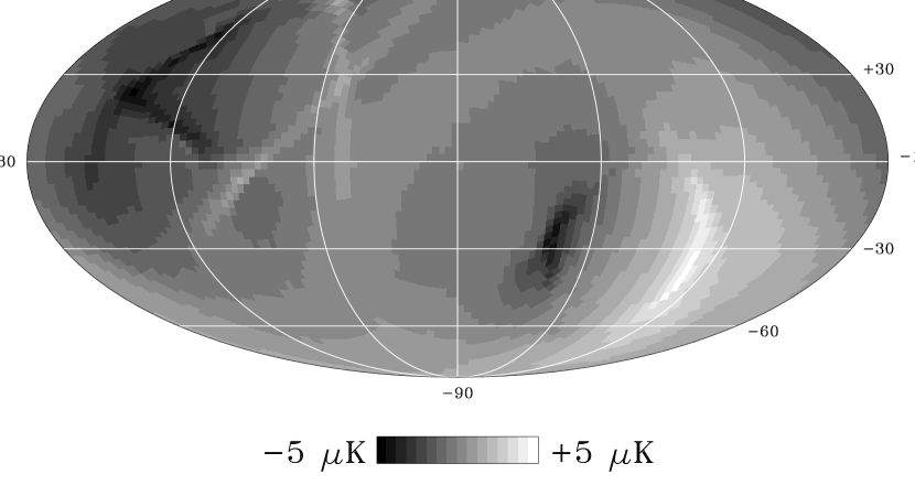
Figure 12: Full sky map of 95% CL upper limits to Earth emission in the 53B channel (Mollweide projection in Galactic coordinates).

Table 9 shows the 95% CL upper limits to Earth emission when the Earth is 1^∘ below the shield. We reject data when the Earth limb is 1^∘ below the shield or higher (3^∘ for the 31.5 GHz channels) but do not otherwise correct the data for the Earth. The Earth signal decreases rapidly as the Earth sets below the shield and falls below the threshold of detection 7^∘ below the shield. Earth emission is not detectable for the majority of the data set: the Earth limb is 7^∘ or more below the shield for 85% of the 4-year mission. We use the elevation dependence of the diffraction model to scale the upper limits at -1^∘ to lower elevation angles, and use this scaled model to map the Earth artifacts in the 4-year sky maps (Eqs. 1 and 2). Figure 12 shows the 95% confidence level limits for Earth emission in the 53B sky map. Since the upper limit is approximately twice the value of the detected signal, the scaled limits at lower elevations are conservative estimates of Earth emission. Earth emission contributes less than 1.8 ${\rm\mu K}$ to the pixel-pixel rms in the sky maps.

An alternate approach is to use the Earth-binned data as the model of Earth emission without reference to any a priori model. This avoids dependence on diffraction estimates but injects the pixel noise of the binned data into the mapping routine. Limits set by this model-independent technique, $\delta T_{Earth}<3.5~{}{{\rm\mu K}}$, are still small compared to the cosmic signal in the maps.

6.2 Moon

The Moon is the brightest source observed by DMR and is the only source visible in the time-ordered data. Away from beam center, its signal is rapidly attenuated by the antenna beam pattern. The beam pattern falls to a local minimum of -39 dB at 21^∘ from beam center, at which point the Moon contributes approximately 150 ${\rm\mu K}$ to the time-ordered data. We reject any datum taken with an antenna pointed within 21^∘ of the Moon and correct all remaining data for lunar emission using an a priori model based on lunar microwave emission properties and the measured DMR beam patterns (§4.1). Uncertainties in the lunar correction are dominated by $\sim$5% systematic uncertainties in the brightness temperature of the Moon, and by $\sim$3% uncertainties in the antenna beam pattern. Residual uncertainties, after correction, are less than 9 ${\rm\mu K}$ in the time-ordered data and less than 0.3 ${\rm\mu K}$ in the maps.

6.3 Sun

A reflective shield protects the radiometers from the Sun, which never directly illuminates the aperture plane. A simple model of solar emission diffracted over the shield yields a limit $Z_{\rm Sun}<2~{}{{\rm\mu K}}$ in the time-ordered data (95% CL). We test for solar emission by binning the data by the solar position relative to the spacecraft axes, similar to the Earth binning in §6.1. We find no evidence for solar emission in the time-ordered data. Solar effects are likely to be dominated by the heating of thermally-sensitive components and not by the direct microwave emission. All solar effects (emission and thermal) are spin modulated and are subsumed in the spin-binned limits in Table 8 (§ 5.3).

6.4 Planets

We correct the time-ordered data for emission from Jupiter, Saturn, and Mars when those planets are within 15^∘ of an antenna beam center. Uncertainties in the applied corrections are dominated by $\sim$10% uncertainties in the brightness temperature of each planet (Kogut et al. 1992). Residual artifacts in the maps, after correction, are less than 0.4 ${\rm\mu K}$. We test for planetary emission by mapping the time-ordered data in a coordinate system centered on the planet Jupiter. Accounting for the change in apparent diameter averaged over the 4 year mission, Jupiter should appear in such a map as an unresolved source with peak amplitude 200 ${\rm\mu K}$. We fit the Jupiter-centered maps to a 7^∘ FWHM Gaussian profile and recover amplitudes $209\pm 139~{}\mu$K, $195\pm 40~{}\mu$K, and $183\pm 55~{}\mu$K antenna temperature at 31.5, 53, and 90 GHz, respectively.

6.5 RFI

Radio-frequency interference (RFI) from ground-based radars, if sufficiently strong, will appear as spikes in the time-ordered data. We have binned the flagged spikes by sub-satellite point and find no correlation with position. We test for RFI from geostationary satellites by mapping the time-ordered data in a coordinate system focused on the geostationary satellite belt, including the effects of parallax. Satellite RFI should appear as an unresolved source on the equator of this coordinate system. We find no such sources to limit $Z_{\rm RFI}<7~{}{{\rm\mu K}}$ in the time-ordered data and $\delta T_{\rm RFI}<0.02~{}{{\rm\mu K}}$ in the sky maps.

7 Miscellaneous Effects

Kogut et al. (1992) place stringent limits on a large number of potential systematic artifacts for the first year of DMR data. We have repeated these analyses for the 4-year data and include their effect in the combined limits to all systematic artifacts; however, we will not discuss each item separately. These effects include the solution convergence of the sparse matrix algorithm, pixel-pixel independence, discrete pixelization, non-uniform sky coverage, cross-talk with the DIRBE and FIRAS instruments, emission from the Sun-Earth shield, zodiacal dust emission, and cosmic-ray hits. Some of these effects are modulated at the spin or orbit periods and are absorbed in the limits in Table 8.

7.1 Attitude Solution

DMR uses the COBE fine aspect attitude solutions based on DIRBE stellar observations. For the first 45 months of the mission, residuals between the attitude solution and known stellar positions are less than 2^′ (68% CL). Fourier analysis of the residuals shows no periodic systematic uncertainties at either the spin or orbit periods; the frequency spectrum is close to white noise. A gyroscope failure on 2 October 1993 led to a wobble in spacecraft azimuth of amplitude $\sim$13^′ which is not included in the attitude solutions. We have simulated the effect of such a wobble in the 4-year DMR sky maps. Attitude artifacts in the maps are less than 0.2 ${\rm\mu K}$ in the pixel-pixel rms.

7.2 Antenna Direction Vectors

The pointing of the 10 DMR antennas relative to the spacecraft body was measured prior to launch. We correct the pointing vectors of both 53B antennas for a 0.25 s telemetry timing offset (Kogut et al. 1992, Bennett et al. 1992a). Observations of the Moon provide a cross-check on the in-flight pointing of the antennas relative to the COBE spacecraft. We find no offsets larger than 16^′, well within our ability to model the centroid of the brightness distribution across the lunar disk. We have made sky maps using the lunar-derived antenna vectors and compared them to the mission maps made with the pre-flight antenna vectors. Systematic artifacts in the maps related to antenna pointing vectors are less than 1.4 ${\rm\mu K}$.

7.3 Lock-in Amplifier Memory

We correct the time-ordered data for the small “memory” of the previous datum caused by the low-pass filter on the lock-in amplifier input,

$$D(t)=D(t_{i})-\alpha D(t_{i-1})$$

where the coefficient $\alpha\approx 0.032$ (Kogut et al. 1992). In the absence of this correction, the lock-in memory creates a positive correlation between neighboring pixels in the sky maps. We compute $\alpha$ for each channel from the autocorrelation of the time-ordered data after correcting the calibrated data for signals from the magnetic susceptibility, eclipse effect, lunar and planetary emission, and the CMB and Earth Doppler dipoles. Table 10 lists the resulting memory coefficients. We simulate the effect of small uncertainties in the applied coefficients. Artifacts in the maps resulting from uncertainties in the memory correction are negligible (less than 0.05 ${\rm\mu K}$).

8 Discussion

We use Eqs. 1 and 2 to make a sky map of each effect before correction and its 95% confidence uncertainty after our best correction (if any) is applied. Note that the temperatures in these maps are highly correlated from pixel to pixel: the spatial pattern is fixed, so that the residual (if any) across the DMR sky maps will be given by scaling the entire upper limit map in the range [-1, 1].

We expand each systematic error map in spherical harmonics,

$$T(\theta,\phi)~{}=~{}\sum_{\ell m}~{}a_{\ell m}Y_{\ell m}(\theta,\phi)$$

and calculate the multipole amplitudes

$$(\Delta T_{\ell})^{2}=\frac{1}{4\pi}\sum_{m}|a_{\ell m}|^{2}$$

for each map. Tables 11 through 16 present the rms, peak-peak amplitude, and multipole amplitudes $\Delta T_{\ell}$ for each systematic effect. The uncertainties in the potential systematic artifacts are largely independent; we adopt the quadrature sum of each column as the upper limit for the combined effects of all systematics. Note that this is not equivalent to adding the individual maps and then deriving $\Delta T_{\ell}$. Tables 11 through 16 list only the largest uncertainties; the row labelled “Other” contains the quadrature sum for all other systematics. This entry includes over a dozen individual effects, such as attitude and pointing errors, calibration drifts, lock-in amplifier memory, orbitally modulated effects, planetary emission, and artifacts from the map algorithm and pixelization. See Kogut et al. (1992) for a complete listing of these minor effects.

Upper limits on the combined effect of all systematics in the pixel-pixel rms of the 4-year DMR sky maps range from 5.4 ${\rm\mu K}$ in the 31B channel (which contains only 21 months of “quiet” data) to 1.9 ${\rm\mu K}$ in the 90B channel. Upper limits on the rms quadrupole amplitude $\Delta T_{2}$ range from 3.8 ${\rm\mu K}$ to 1.1 ${\rm\mu K}$. The power drops rapidly at higher multipole moments $\ell$.

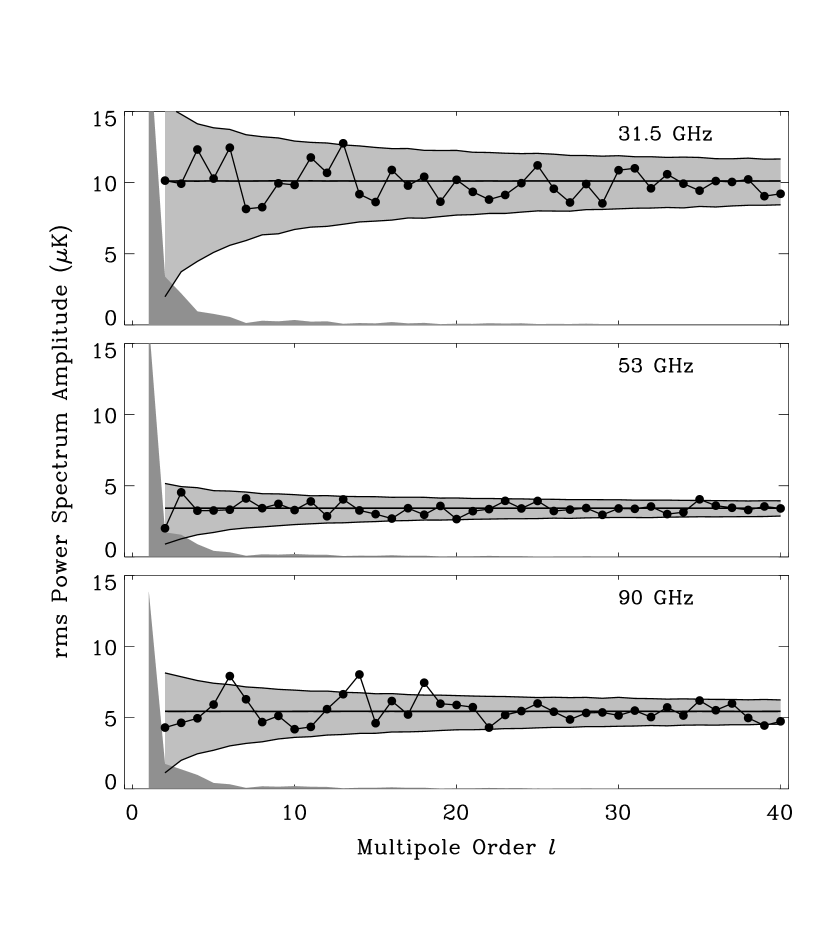
Figure 13: Power spectrum of the 4-year (A-B)/2 difference maps compared to the instrument noise and upper limits on the combined systematic uncertainties. Points represent the power spectrum of the (A-B)/2 map, while the light gray band represents the 95% CL range of power from Monte Carlo simulations of instrument noise. The dark gray band shows 95% confidence level upper limits to the quadrature sum of systematic effects.

We test for additional systematic artifacts in the sky maps by analyzing various “difference map” linear combinations in which celestial emission cancels, leaving instrument noise and (potentially) systematic effects. Examples are the (A-B)/2 differences between the A and B channels at each frequency, or similar maps made by differencing a single channel mapped in different time ranges (second year minus first year). Figure 13 shows the power spectrum of the 4-year (A-B)/2 difference maps compared to the expected instrument noise and the 95% confidence upper limits on combined systematic effects. The gray band represents the 95% CL range of power from instrument noise, determined by Monte Carlo simulation using the observation pattern of each channel. The power spectra of the difference maps are in agreement with the expected instrument noise and show no statistically significant excursions. The upper limits to power from combined systematics are well below the noise limits: systematic artifacts do not limit analysis of the DMR sky maps.

9 Conclusions

We use in-flight data from the full 4 year mission to obtain estimates of potential systematic effects in the DMR time-ordered data, and use the mapping software to create maps of each effect and its associated 95% confidence level uncertainty. The largest effect known to exist in the time-ordered data is the instrument response to an external magnetic field. We correct for this magnetic susceptibility using a linear vector coupling between the radiometer orientation and the Earth’s magnetic field. The uncertainty in the correction is dominated by the instrument noise in the case of weak coupling and uncertainty in the local magnetic field for larger couplings.

With four years of data, we detect emission from the Earth at the level $42\pm 15~{}{{\rm\mu K}}$ when the Earth is 1^∘ below the Sun/Earth shield. We reject data when the Earth is 1^∘ below the shield or higher, but do not otherwise correct for this emission. Emission from the Earth agrees well with a simple diffraction model over the limited range of elevation angles for which we detect the Earth. We use the elevation dependence of the diffraction model to scale the detection at -1^∘ to lower elevation angles when deriving upper limits to Earth artifacts in the 4-year sky maps.

We correct the calibrated time-ordered data for the known systematic effects (Table 1) and bin the data by the spacecraft spin angle relative to the Sun. We find no evidence for additional systematic effects modulated at the spin period. Our ability to detect weak signals with this method is limited by the instrument noise; upper limits to spin-modulated artifacts in the maps determined from the spin-binned data are determined by the instrument noise and not by a detected signal.

We detect an orbitally modulated signal in all channels during the 2-month “eclipse season” surrounding the June solstice, when the spacecraft flies through the Earth’s shadow over the Antarctic each orbit. The detection of thermal gain variations during the same time range provides a plausible mechanism for this effect. We correct the time-ordered data using an empirical model based on variations in unregulated spacecraft temperature and voltage signals, which provide templates for the time variation less affected by telemetry digitization than the housekeeping signals on the amplifiers themselves. The model removes about 2/3 of the signal. The residual is large enough in the 31A and 31B channels that the 4-year data would be adversely affected by including the corrected data with the residual signal. We do not use data during the eclipse season for the 31A and 31B channels.

Observations of the Moon and the Doppler dipoles from the motion of the satellite about the Earth and the Earth about the Solar system barycenter demonstrate that the pre-flight calibration is accurate within its uncertainties. On-board noise sources track the gain correctly within 0.2% per year. Artifacts from calibration errors are negligible. The 70 ${\rm\mu K}$ Doppler signal from the orbital motion of the spacecraft about the Earth and the 200 ${\rm\mu K}$emission from Jupiter serve as convenient test patterns in the appropriate specialized coordinate systems. DMR observes both signals with good signal to noise ratio.

We map the pattern of artifacts in the sky from the 95% confidence level uncertainty in each potential systematic effect and analyze these maps as though they were maps of the CMB. The quadrature sum of the combined upper limits ranges from 5.4 ${\rm\mu K}$ to 1.9 ${\rm\mu K}$ in the pixel-pixel rms, and from 3.8 ${\rm\mu K}$ to 1.1 ${\rm\mu K}$ for the rms quadrupole amplitude. The power drops rapidly at higher multipole moments $\ell$. The power spectra of the 4-year (A-B)/2 difference maps are consistent with the distribution of instrument noise in the maps and show no evidence for systematic artifacts. Upper limits to power from combined systematics in the DMR 4-year sky maps are well below the noise limits: systematic artifacts do not limit analysis of the DMR sky maps.

References

Barker, F.S., et al. 1986, EOS, 67, 523

Bennett, C.L., et al. 1992a, ApJ, 391, 466

— 1992b, ApJ, 396, L7

— 1994, ApJ, 436, 423

— 1996, ApJ Letters, submitted

Boggess, N.W., et al. 1992, ApJ, 397, 420

Fixsen, D.J., Gales, J.M., Mather, J.C., Shafer, R.A., & Wright, E.L. 1996, ApJ, submitted

Jackson, P.D., et al. 1996, in preparation

— 1992, in Astronomical Data Analysis Software and Systems I, ed. W. Worrall, C. Biemesderfer, and J. Barnes, (ASP:San Francisco), 382

Janssen, M.A., & Gulkis, S. 1992, in The Infrared and Submillimeter Sky After COBE, ed. M. Signore & C. Dupraz (Dordrecht: Kluwer), 391

Lineweaver, C.H., Smoot, G.F., Bennett, C.L., Wright, E.L., Tenorio, L., Kogut, A., Keegstra, P.B., Hinshaw, G., & Banday, A.J. 1994, ApJ, 436, 452

Keihm, S.J. 1982, Icarus, 53, 570

Keihm, S.J. & Gary, B.L. 1979, Proc. 10th Lun. Planet Sci. Conf., 2311

Keihm, S.J. & Langseth, M.G. 1975, Icarus, 24, 211

Kogut, A., et al. 1992, ApJ, 401, 1

—, Banday, A.J., Bennett, C.L., Górski, K.M., Hinshaw, G., & Reach, W.T. 1996a, ApJ, in press

—, Hinshaw, G., Banday, A.J., Bennett, C.L., Górski, K.M., & Smoot, G.F. 1996b, APJ Letters, submitted

Peebles, P.J.E., & Wilkinson, D.T. 1968, Phys Rev, 174, 2168

Toral, M.A., Ratliff, R.B., Lecha, M.C., Maruschak, J.G., Bennett, C.L., & Smoot, G.F. 1990, IEEE Trans. Ant. Prop., 37, 171

Torres, S., et al. 1989, in Data Analysis in Astronomy III, ed. V. Di Gesu, L. Scarsi, & M.C. Maccarone (New York: Plenum), 319

Smoot, G.F., et al. 1990, ApJ, 360, 685

— et al. 1992, ApJ, 391, L1

Wright, E.L., et al. 1994, ApJ, 420, 1

Table 1: Cuts and Corrections Made to DMR Time-Ordered Data

Effect	Cuta	Correction
No telemetry	Yes (0.4%)	No
Spike in data	Yes (0.3%)	No
Offscale data	Yes (0.3%)	No
Bad attitude	Yes (0.7%)	No
Unstable Noise	Yes (4.2%)b	No
Calibration	Yes (2.2%)	No
Earth emission	Yes (5.0%)	No
Lunar emission	Yes (4.6%)	Yes
Planetary emission	No	Yes
Lock-in amplifier memory	No	Yes
Magnetic susceptibility	No	Yes
Earth Doppler	No	Yes
Satellite Doppler	No	Yes
Seasonal effects	Yes (26.0%)c	Yes

^a Numbers in parentheses are the fraction of data rejected for each cut.
^b 31B channel only.
^c 31A and 31B channels only.

Table 2: Calibration Summary^a

Channel	Absolute Calibration		Relative	Linear Drift	Orbit Drift	Spin Drift
	Ground (%)	Flight (%)	A/B (%)	(percent yr-1)	$(10^{5}~{}\Delta{\cal G}/{\cal G})$	$(10^{7}~{}\Delta{\cal G}/{\cal G})$
31A	0.0 $\pm$ 2.5	+2.2 $\pm$ 3.0	0.40 $\pm$ 0.05	+0.23 $\pm$ 0.33	6.7	15
31B	0.0 $\pm$ 2.3	+1.6 $\pm$ 3.8		+0.03 $\pm$ 0.81	22.5	55
53A	0.0 $\pm$ 0.7	-0.8 $\pm$ 1.2	0.27 $\pm$ 0.02	-0.12 $\pm$ 0.03	2.6	20
53B	0.0 $\pm$ 0.7	-0.1 $\pm$ 1.4		-0.11 $\pm$ 0.11	2.4	13
90A	0.0 $\pm$ 2.0	+2.6 $\pm$ 2.5	0.01 $\pm$ 0.03	-0.12 $\pm$ 0.04	5.4	13
90B	0.0 $\pm$ 1.3	-1.7 $\pm$ 1.8		-0.20 $\pm$ 0.11	7.2	8

^a These corrections to the ground calibration have not been applied to the data. Uncertainties are 68% confidence level except for the spin and orbit drifts, which are 95% confidence upper limits.

Table 3: Absolute Calibration Compared to Noise Sources

Channel	Ground	Doppler	Moon
31A	1.000 $\pm$ 0.025	1.022 $\pm$ 0.030	1.021 $\pm$ 0.038
31B	1.000 $\pm$ 0.023	1.116 $\pm$ 0.058	1.016 $\pm$ 0.038
53A	1.000 $\pm$ 0.007	0.992 $\pm$ 0.012	1.021 $\pm$ 0.054
53B	1.000 $\pm$ 0.007	0.999 $\pm$ 0.014	1.018 $\pm$ 0.054
90A	1.000 $\pm$ 0.020	1.026 $\pm$ 0.025	1.014 $\pm$ 0.063
90B	1.000 $\pm$ 0.013	0.983 $\pm$ 0.018	1.013 $\pm$ 0.063

Table 4: Relative A/B Calibration Compared to Noise Sources

Frequency	Ground	Doppler	Moon
31	1.000 $\pm$ 0.026	0.915 $\pm$ 0.054	1.0040 $\pm$ 0.0005
53	1.000 $\pm$ 0.003	0.993 $\pm$ 0.018	1.0027 $\pm$ 0.0002
90	1.000 $\pm$ 0.010	1.044 $\pm$ 0.032	1.0001 $\pm$ 0.0003

Table 5: Linear Calibration Drifts

Channel	NS Ratio	CMB Dipole	Moon
	(percent yr-1)	(percent yr-1)	(percent yr-1)
31A	+0.468 $\pm$ 0.004	+0.365 $\pm$ 0.278	-0.140 $\pm$ 0.024
31B	-0.576 $\pm$ 0.015	+0.947 $\pm$ 1.281	-0.293 $\pm$ 0.029
53A	-0.139 $\pm$ 0.001	-0.091 $\pm$ 0.122	-0.131 $\pm$ 0.009
53B	-0.191 $\pm$ 0.001	+0.023 $\pm$ 0.139	-0.147 $\pm$ 0.011
90A	-0.099 $\pm$ 0.003	-0.173 $\pm$ 0.209	-0.098 $\pm$ 0.018
90B	-0.131 $\pm$ 0.001	-0.325 $\pm$ 0.174	-0.140 $\pm$ 0.015

Table 6: Magnetic Susceptibility (mK G^-1)

Channel	$\beta_{X}$	$\beta_{R}$	$\beta_{T}$
31A	-0.173 $\pm$ 0.018	+0.262 $\pm$ 0.039	-0.196 $\pm$ 0.067
31B	+0.284 $\pm$ 0.024	+0.224 $\pm$ 0.054	+0.011 $\pm$ 0.089
53A	-1.514 $\pm$ 0.006	-0.081 $\pm$ 0.013	-0.881 $\pm$ 0.022
53B	+0.087 $\pm$ 0.006	-0.408 $\pm$ 0.015	-0.192 $\pm$ 0.025
90A	-0.135 $\pm$ 0.010	-1.175 $\pm$ 0.024	-0.334 $\pm$ 0.040
90B	-0.003 $\pm$ 0.007	+0.140 $\pm$ 0.017	-0.136 $\pm$ 0.028

Table 7: Eclipse Coefficients for Empirical Model

Channel	Thermal ( mK du-1)a		Voltage (mK du-1)a
	During Eclipse	Excluding Eclipse	During Eclipse	Excluding Eclipse
31A	+0.442 $\pm$ 0.006	+0.046 $\pm$ 0.029	+0.311 $\pm$ 0.015	+0.018 $\pm$ 0.019
31B	+0.147 $\pm$ 0.008	-0.011 $\pm$ 0.038	+0.262 $\pm$ 0.019	-0.008 $\pm$ 0.027
53A	-0.022 $\pm$ 0.002	+0.001 $\pm$ 0.007	+0.013 $\pm$ 0.004	-0.002 $\pm$ 0.007
53B	-0.069 $\pm$ 0.003	-0.010 $\pm$ 0.010	-0.011 $\pm$ 0.004	+0.001 $\pm$ 0.007
90A	+0.042 $\pm$ 0.004	+0.032 $\pm$ 0.018	+0.024 $\pm$ 0.008	+0.009 $\pm$ 0.011
90B	0.000 $\pm$ 0.003	-0.018 $\pm$ 0.011	0.000 $\pm$ 0.005	+0.008 $\pm$ 0.011

^a Temperature and voltage housekeeping signals are processed in digitized telemetry units (du).

Table 8: 95% Confidence Upper Limits From Orbit- and Spin-Modulated Effects^a

Channel	Spin Period	Orbit Period	Orbit Period
	All Data	During Eclipse	Excluding Eclipse
	(${\rm\mu K}$)	(${\rm\mu K}$)	(${\rm\mu K}$)
31A	34	577	19
31B	41	489	47
53A	11	33	14
53B	10	19	12
90A	18	73	24
90B	8	21	18

^a All values are in units of antenna temperature.

Table 9: 95% Confidence Upper Limits From Earth Emission in Time-Ordered Data^a

Channel	1∘ below shieldb	7∘ below shieldc
	(${\rm\mu K}$)	(${\rm\mu K}$)
31A	179	26
31B	183	27
53A	85	8
53B	89	10
90A	136	10
90B	113	7

^a All values are in units of antenna temperature.
^b Direct fit to binned data 1^∘ below the shield.
^c Values at -7^∘ are taken from the values at -1^∘ (column (2)), scaled to -7^∘ using diffraction model.

Table 10: Lock-in Amplifier Memory

Channel	Lock-in Memory Amplitude
	(percent of signal)
31A	3.220 $\pm$ 0.003
31B	3.146 $\pm$ 0.004
53A	3.203 $\pm$ 0.003
53B	3.172 $\pm$ 0.003
90A	3.110 $\pm$ 0.003
90B	3.139 $\pm$ 0.004

Table 11: Systematic Effects for Channel 31A^a

Effect	P-Pb	rmsc	$\Delta T_{1}$	$\Delta T_{2}$	$\Delta T_{3}$	$\Delta T_{4}$	$\Delta T_{5}$	$\Delta T_{6}$	$\Delta T_{7}$	$\Delta T_{8}$
	($\mu$K)	($\mu$K)	($\mu$K)	($\mu$K)	($\mu$K)	($\mu$K)	($\mu$K)	($\mu$K)	($\mu$K)	($\mu$K)
Channel 31A Before Correction
$\beta_{X}$	6.7	0.4	0.2	0.1	0.1	0.0	0.1	0.0	0.0	0.0
$\beta_{R}$	31.9	6.5	1.1	6.1	0.5	1.6	0.7	1.0	0.2	0.5
$\beta_{T}$	17.4	2.9	18.4	1.6	1.9	0.7	0.9	0.3	0.1	0.2
Earth	7.0	1.2	1.5	0.9	0.4	0.4	0.3	0.2	0.0	0.1
Moon	7.9	1.6	0.0	1.2	0.0	0.4	0.1	0.3	0.0	0.5
Doppler	85.6	13.4	65.3	5.6	10.4	1.8	3.5	1.4	0.8	0.7
Spin	11.1	1.5	5.3	0.6	1.0	0.4	0.4	0.3	0.0	0.2
Other	81.3	9.1	2.3	0.8	0.4	0.5	0.4	0.5	0.4	0.5
Totald	124.7	17.9	68.2	8.6	10.6	2.7	3.7	1.8	0.9	1.2
Channel 31A After Correctione
$\beta_{X}$	1.6	0.1	0.1	0.0	0.0	0.0	0.0	0.0	0.0	0.0
$\beta_{R}$	10.3	2.1	0.4	2.0	0.2	0.5	0.2	0.3	0.1	0.2
$\beta_{T}$	12.1	2.0	12.8	1.1	1.3	0.5	0.6	0.2	0.1	0.1
Earth	7.6	1.3	1.6	1.0	0.4	0.4	0.3	0.2	0.0	0.2
Moon	0.9	0.2	0.0	0.1	0.0	0.1	0.0	0.0	0.0	0.1
Doppler	4.3	0.7	3.3	0.3	0.5	0.1	0.2	0.1	0.0	0.0
Spin	23.2	3.1	11.1	1.3	2.0	0.8	0.8	0.7	0.1	0.4
Other	15.6	1.4	2.5	0.5	0.5	0.3	0.2	0.2	0.1	0.3
Totald	33.4	4.7	17.5	2.8	2.5	1.2	1.1	0.9	0.2	0.6

^a All results are in units of antenna temperature.
^b Peak to peak amplitude in the map after best-fit dipole is removed.
^c Pixel to pixel standard deviation after best-fit dipole is removed.
^d Quadrature sum of the individual effects in each column.
^e 95% confidence upper limits.

Table 12: Systematic Effects for Channel 31B^a

Effect	P-P	rms	$\Delta T_{1}$	$\Delta T_{2}$	$\Delta T_{3}$	$\Delta T_{4}$	$\Delta T_{5}$	$\Delta T_{6}$	$\Delta T_{7}$	$\Delta T_{8}$
	($\mu$K)	($\mu$K)	($\mu$K)	($\mu$K)	($\mu$K)	($\mu$K)	($\mu$K)	($\mu$K)	($\mu$K)	($\mu$K)
Channel 31B Before Correction
$\beta_{X}$	8.4	0.5	0.3	0.1	0.1	0.1	0.1	0.1	0.0	0.0
$\beta_{R}$	26.3	5.1	0.6	4.5	0.7	1.6	0.6	0.5	0.1	0.4
$\beta_{T}$	0.0	0.0	0.0	0.0	0.0	0.0	0.0	0.0	0.0	0.0
Earth	11.5	1.6	0.5	1.5	0.3	0.3	0.3	0.2	0.0	0.1
Moon	8.5	1.6	0.1	1.3	0.0	0.4	0.0	0.3	0.0	0.5
Doppler	97.1	15.6	66.5	6.1	12.0	2.7	4.6	2.2	1.2	1.2
Spin	8.6	1.1	4.1	0.5	0.8	0.3	0.3	0.3	0.0	0.2
Other	95.9	10.9	0.7	0.7	0.3	0.5	0.3	0.5	0.4	0.5
Total	140.2	19.9	66.6	7.9	12.1	3.2	4.7	2.3	1.3	1.5
Channel 31B After Correction
$\beta_{X}$	1.7	0.1	0.1	0.0	0.0	0.0	0.0	0.0	0.0	0.0
$\beta_{R}$	13.1	2.5	0.3	2.3	0.4	0.8	0.3	0.3	0.1	0.2
$\beta_{T}$	0.0	0.0	0.0	0.0	0.0	0.0	0.0	0.0	0.0	0.0
Earth	13.0	1.8	0.6	1.6	0.4	0.3	0.3	0.2	0.1	0.1
Moon	0.9	0.2	0.0	0.1	0.0	0.1	0.0	0.0	0.0	0.1
Doppler	4.5	0.7	3.1	0.3	0.6	0.1	0.2	0.1	0.1	0.1
Spin	28.2	3.7	13.4	1.5	2.5	0.9	1.0	0.9	0.1	0.5
Other	22.1	2.6	2.8	0.5	1.1	0.4	0.5	0.3	0.2	0.3
Total	40.6	5.6	14.1	3.2	2.8	1.4	1.2	1.0	0.2	0.6

^a All results are in units of antenna temperature. Columns are the same as Table 11.

Table 13: Systematic Effects for Channel 53A^a

Effect	P-P	rms	$\Delta T_{1}$	$\Delta T_{2}$	$\Delta T_{3}$	$\Delta T_{4}$	$\Delta T_{5}$	$\Delta T_{6}$	$\Delta T_{7}$	$\Delta T_{8}$
	($\mu$K)	($\mu$K)	($\mu$K)	($\mu$K)	($\mu$K)	($\mu$K)	($\mu$K)	($\mu$K)	($\mu$K)	($\mu$K)
Channel 53A Before Correction
$\beta_{X}$	32.9	2.2	5.1	0.4	0.8	0.4	0.4	0.3	0.1	0.1
$\beta_{R}$	6.3	1.0	0.6	0.6	0.2	0.7	0.2	0.2	0.0	0.1
$\beta_{T}$	101.0	15.7	92.8	7.6	11.9	3.0	2.7	1.7	0.5	1.0
Earth	6.6	0.7	0.5	0.6	0.2	0.2	0.1	0.1	0.0	0.1
Moon	7.1	1.5	0.0	1.2	0.0	0.4	0.0	0.3	0.0	0.5
Doppler	70.9	10.9	50.5	6.8	6.7	1.8	3.0	1.9	0.5	1.3
Spin	3.3	0.4	1.6	0.2	0.3	0.1	0.1	0.1	0.0	0.1
Other	37.3	3.7	1.0	1.0	0.4	0.6	0.3	0.5	0.4	0.5
Total	133.6	19.7	105.7	10.4	13.7	3.7	4.1	2.6	0.8	1.8
Channel 53A After Correction
$\beta_{X}$	4.3	0.3	0.7	0.1	0.1	0.1	0.1	0.0	0.0	0.0
$\beta_{R}$	2.2	0.4	0.2	0.2	0.1	0.3	0.1	0.1	0.0	0.0
$\beta_{T}$	14.3	2.2	13.2	1.1	1.7	0.4	0.4	0.2	0.1	0.2
Earth	7.9	0.9	0.6	0.8	0.2	0.2	0.1	0.1	0.0	0.1
Moon	0.9	0.2	0.0	0.1	0.0	0.1	0.0	0.0	0.0	0.1
Doppler	1.2	0.2	0.7	0.1	0.1	0.0	0.1	0.0	0.0	0.0
Spin	7.6	1.0	3.6	0.4	0.7	0.3	0.3	0.2	0.0	0.1
Other	10.6	1.0	0.9	0.7	0.1	0.2	0.1	0.2	0.1	0.1
Total	21.5	2.8	13.7	1.6	1.8	0.6	0.5	0.4	0.2	0.3

^a All results are in units of antenna temperature. Columns are the same as Table 11.

Table 14: Systematic Effects for Channel 53B^a

Effect	P-P	rms	$\Delta T_{1}$	$\Delta T_{2}$	$\Delta T_{3}$	$\Delta T_{4}$	$\Delta T_{5}$	$\Delta T_{6}$	$\Delta T_{7}$	$\Delta T_{8}$
	($\mu$K)	($\mu$K)	($\mu$K)	($\mu$K)	($\mu$K)	($\mu$K)	($\mu$K)	($\mu$K)	($\mu$K)	($\mu$K)
Channel 53B Before Correction
$\beta_{X}$	1.1	0.1	0.1	0.0	0.0	0.0	0.0	0.0	0.0	0.0
$\beta_{R}$	31.5	5.3	2.8	3.2	1.2	3.6	0.9	0.8	0.2	0.5
$\beta_{T}$	22.1	3.4	20.3	1.7	2.6	0.7	0.6	0.4	0.1	0.2
Earth	6.6	0.8	0.6	0.7	0.2	0.2	0.1	0.1	0.0	0.1
Moon	7.2	1.6	0.0	1.2	0.0	0.4	0.0	0.2	0.0	0.5
Doppler	70.5	10.9	50.5	6.8	6.7	1.8	3.0	1.9	0.4	1.3
Spin	2.1	0.3	1.0	0.1	0.2	0.1	0.1	0.1	0.0	0.0
Other	41.9	4.3	2.7	1.3	0.4	0.6	0.3	0.5	0.4	0.5
Total	91.2	13.4	54.6	7.9	7.3	4.1	3.2	2.2	0.6	1.5
Channel 53B After Correction
$\beta_{X}$	0.2	0.0	0.0	0.0	0.0	0.0	0.0	0.0	0.0	0.0
$\beta_{R}$	11.1	1.9	1.0	1.1	0.4	1.3	0.3	0.3	0.1	0.2
$\beta_{T}$	6.4	1.0	5.8	0.5	0.8	0.2	0.2	0.1	0.0	0.1
Earth	8.7	1.0	0.8	0.9	0.2	0.2	0.2	0.1	0.0	0.1
Moon	0.9	0.2	0.0	0.2	0.0	0.1	0.0	0.0	0.0	0.1
Doppler	1.2	0.2	0.7	0.1	0.1	0.0	0.1	0.0	0.0	0.0
Spin	7.1	0.9	3.4	0.4	0.6	0.2	0.2	0.2	0.0	0.1
Other	17.3	1.5	2.6	1.0	0.2	0.3	0.1	0.2	0.2	0.2
Total	24.3	2.9	7.4	1.9	1.1	1.4	0.5	0.4	0.2	0.3

^a All results are in units of antenna temperature. Columns are the same as Table 11.

Table 15: Systematic Effects for Channel 90A^a

Effect	P-P	rms	$\Delta T_{1}$	$\Delta T_{2}$	$\Delta T_{3}$	$\Delta T_{4}$	$\Delta T_{5}$	$\Delta T_{6}$	$\Delta T_{7}$	$\Delta T_{8}$
	($\mu$K)	($\mu$K)	($\mu$K)	($\mu$K)	($\mu$K)	($\mu$K)	($\mu$K)	($\mu$K)	($\mu$K)	($\mu$K)
Channel 90A Before Correction
$\beta_{X}$	4.9	0.4	1.6	0.1	0.2	0.1	0.1	0.0	0.0	0.0
$\beta_{R}$	89.3	15.1	7.9	9.2	3.4	10.4	2.7	2.1	0.5	1.3
$\beta_{T}$	37.8	5.9	35.0	2.9	4.5	1.1	1.0	0.6	0.2	0.4
Earth	4.8	0.6	0.5	0.5	0.1	0.2	0.1	0.1	0.0	0.1
Moon	8.4	1.8	0.1	1.4	0.0	0.5	0.0	0.3	0.0	0.6
Doppler	62.3	9.6	44.3	5.9	5.9	1.6	2.7	1.6	0.4	1.1
Spin	4.9	0.6	2.3	0.3	0.4	0.2	0.2	0.2	0.0	0.1
Other	51.8	5.3	1.7	0.9	0.3	0.5	0.3	0.5	0.3	0.4
Total	126.9	19.7	57.1	11.4	8.2	10.6	3.9	2.8	0.8	2.0
Channel 90A After Correction
$\beta_{X}$	1.0	0.1	0.3	0.0	0.0	0.0	0.0	0.0	0.0	0.0
$\beta_{R}$	12.3	2.1	1.1	1.3	0.5	1.4	0.4	0.3	0.1	0.2
$\beta_{T}$	10.3	1.6	9.5	0.8	1.2	0.3	0.3	0.2	0.1	0.1
Earth	9.4	1.2	1.0	1.0	0.2	0.3	0.2	0.2	0.1	0.1
Moon	1.4	0.3	0.0	0.2	0.0	0.1	0.0	0.1	0.0	0.1
Doppler	2.6	0.4	1.8	0.3	0.2	0.1	0.1	0.1	0.0	0.1
Spin	12.1	1.6	5.8	0.7	1.1	0.4	0.4	0.4	0.0	0.2
Other	15.4	1.0	1.6	0.7	0.1	0.2	0.1	0.2	0.1	0.2
Total	27.2	3.5	11.5	2.0	1.7	1.6	0.7	0.6	0.2	0.4

^a All results are in units of antenna temperature. Columns are the same as Table 11.

Table 16: Systematic Effects for Channel 90B^a

Effect	P-P	rms	$\Delta T_{1}$	$\Delta T_{2}$	$\Delta T_{3}$	$\Delta T_{4}$	$\Delta T_{5}$	$\Delta T_{6}$	$\Delta T_{7}$	$\Delta T_{8}$
	($\mu$K)	($\mu$K)	($\mu$K)	($\mu$K)	($\mu$K)	($\mu$K)	($\mu$K)	($\mu$K)	($\mu$K)	($\mu$K)
Channel 90B Before Correction
$\beta_{X}$	0.1	0.0	0.0	0.0	0.0	0.0	0.0	0.0	0.0	0.0
$\beta_{R}$	10.7	1.8	0.9	1.1	0.4	1.2	0.3	0.3	0.1	0.2
$\beta_{T}$	15.4	2.4	14.2	1.2	1.8	0.5	0.4	0.3	0.1	0.2
Earth	5.3	0.6	0.5	0.5	0.1	0.2	0.1	0.1	0.0	0.1
Moon	9.4	2.0	0.1	1.5	0.0	0.6	0.0	0.3	0.0	0.6
Doppler	62.7	9.6	44.3	5.9	5.9	1.6	2.7	1.6	0.5	1.2
Spin	0.1	0.0	0.0	0.0	0.0	0.0	0.0	0.0	0.0	0.0
Other	43.1	4.3	1.4	0.8	0.3	0.5	0.3	0.4	0.3	0.4
Total	79.1	11.1	46.5	6.4	6.2	2.2	2.7	1.8	0.6	1.4
Channel 90B After Correction
$\beta_{X}$	0.5	0.0	0.1	0.0	0.0	0.0	0.0	0.0	0.0	0.0
$\beta_{R}$	2.9	0.5	0.3	0.3	0.1	0.3	0.1	0.1	0.0	0.0
$\beta_{T}$	6.7	1.0	6.2	0.5	0.8	0.2	0.2	0.1	0.0	0.1
Earth	7.8	0.9	0.7	0.8	0.2	0.2	0.1	0.1	0.0	0.1
Moon	1.5	0.3	0.0	0.3	0.0	0.1	0.0	0.1	0.0	0.1
Doppler	1.8	0.3	1.2	0.2	0.2	0.1	0.1	0.1	0.0	0.0
Spin	5.4	0.7	2.6	0.3	0.5	0.2	0.2	0.2	0.0	0.1
Other	11.2	0.8	1.3	0.5	0.2	0.2	0.1	0.1	0.1	0.1
Total	16.6	1.9	7.0	1.2	1.0	0.5	0.3	0.3	0.1	0.2

^a All results are in units of antenna temperature. Columns are the same as Table 11.

Figure 1: Instrument noise for the 53B radiometer, sorted by integration time. The time-ordered data are first sorted by the orientation of the two antennas, and all observations with the spacecraft in a fixed position in inertial coordinates are combined. Temperature patterns fixed on the sky affect the mean temperature difference of each such pixel combination but do not affect the standard deviation. The plot shows the uncertainty in the mean values (“instrument noise”). There is no evidence for a noise floor caused by non-celestial signals.

Figure 3: Modulation of the CMB dipole resulting from the Doppler effect of the Earth’s orbital motion about the Sun (channel 53B). Each datum represents 5 days. The amplitude of the modulation provides an independent absolute calibration.

Figure 4: 53 GHz (A+B)/2 summed data mapped in a coordinate system fixed with respect to the satellite orbital velocity vector. The data have been binned by angle relative to the COBE orbital velocity vector and corrected for the 0${\hbox to0.0pt{.\hss}}^{\circ}$5 smoothing of the DMR beam. The attitude control system prevents full coverage in this coordinate system. The Doppler effect provides a known signal with amplitude $\Delta T/T\sim 10^{-5}$.

Figure 7: Calibration signals binned at the orbit period for eclipse data (left panels) and non-eclipse data (right panels). (top) Noise source calibration residuals. (middle) Total power residuals. (bottom) Lock-in amplifier temperature. The noise source and total power plots during eclipse season are overlaid with the scaled IPDU thermistor temperature to demonstrate the similarity of the wave forms (see text).

Figure 8: Magnetic and celestial signals vs time for 53B channel. (top) Magnetic signal $Z_{\rm magnetic}(t)$ from the Earth’s field. The spin and orbit modulation are clearly apparent. (bottom) Celestial signal from an unresolved source (the Moon). The orbital modulation results from sweeping the antenna beam pattern across the source at varying angles from beam center. The magnetic signal is easily distinguished from fixed celestial sources.

Figure 11: Amplitude of Earth emission in time-ordered data as a function of Earth limb elevation angle. The azimuthal variation from the beam patterns has been fitted to the Earth-binned data in a strip one pixel high. Earth emission falls rapidly as the Earth sets below the shield. We reject data for which the Earth limb is 1^∘ below the shield or higher (3^∘ for the 31A and 31B channels).