Non–LTE Excitation of H₂ in Magnetised Molecular Shocks

Abstract

The observed H₂ line ratios in OMC–1 and IC443 are not satisfactorily explained by conventional shock excitation models. We consider the microscopic collisional processes implicit in ambipolar diffusion models of magnetised C-shocks and show that non-LTE level populations and emission line ratios are an inevitable consequence of such models. This has important implications for the use of molecular hydrogen lines as diagnostics of shock models in molecular clouds.

1 Introduction

Recent observations of shocked molecular hydrogen, particularly in OMC–1 and IC–443 (Brand et al. 1988, Richter, Graham & Watt 1995), show H₂ excitation line ratios that have proven difficult to model. The original models of these regions involved magnetic shocks, and were able to explain the presence of relatively high velocity shocks (over 25 km s^-1) which did not lead to molecular destruction (Draine 1980). These models, however, could not explain the observed line ratios. New models for these regions suggest that the observed populations could result from the complex cooling zones which follow partially–dissociative shocks (Brand et al. 1988) or result from emission in the wake of fast–moving clumps of material (Smith 1991). However, no model has yet been able to explain the uniformity of the emission over large regions and why it appears to be so similar for two different sources. It is possible that a magnetic shock model which incorporated non–thermal effects could help to explain both the line widths and ratios observed.

Draine (1980) and Draine, Roberge & Dalgarno (1983, hereafter DRD83) studied magnetohydrodynamic (MHD) shock models, whereby the shock structure is altered by the streaming of ionised species ahead of the neutral shock front due to magnetic field compression. Both papers note, however, that the low densities present ($<10^{6}$cm^-3) mean that it is uncertain if LTE can be assumed throughout these shocks. This uncertainty is strongest if particles have anomalous excitation populations, something which will happen whenever ions collide with neutrals at highly non–thermal velocities, an integral part of the differential streaming (ambipolar diffusion) process at the heart of MHD shocks. In such a collision, and in the collisional cascade which follows, there may be significant non–thermal excitation of the neutral particles, leading to enhanced emission from lines not normally seen at the local kinetic temperature. In this paper we describe detailed Monte–Carlo simulations of the microscopic processes of momentum transfer between the different component species in the shock to see what effect such non–LTE processes have on the total emission and the relative line intensity ratios emitted from a magnetised shock. These results are compared with observation, and found to have many of the same properties without resort to complex geometry.

2 The Model

In the shocked regions of interest H₂ is the principal coolant (Smith, 1991). Since it is the ratios of H₂ emission lines that are of interest and other species have relative abundances of less than 10^-4, it is reasonable to limit the chemical composition of the neutral gas considered to just this one species. More complex chemistry could, in principal, be included but is unlikely to affect the results significantly.

In ambipolar diffusion models of shocks (Draine 1980, DRD83 for example. See Draine & McKee 1993 for a review) the small number of ions present are forced at relatively high velocity through the bulk neutral gas by electromagnetic forces associated with the compression of the magnetic field in the shock. At the low ionisation fractions in these regions, typically $10^{-4}-10^{-8}$, reasonable assumptions about the local ambient magnetic field show that the “streaming velocity” can be a large fraction of the shock velocity, reaching 20 km s^-1 for a 25 km s^-1 shock, for example. Collisions between the fast moving ions and the neutral molecules transfer momentum and energy to the neutral population thereby accelerating and heating it. In all previous calculations it has been assumed that the neutral population is in LTE, so that the radiation resulting from this heating can be calculated using standard cooling functions and line ratios. However the inital ion-neutral collision is at velocities which are typically very much higher than thermal, and the resulting accelerated neutral molecule will also be very fast moving, as will the second generation of molecules emerging from its next collision, and so on. There will be a cascade of collisions with the velocity roughly halving at each generation, and the number of molecules involved doubling. At least this would be the picture if there was no excitation of internal degrees of freedom in the collisions. The Monte–Carlo simulations described in this paper model collisional cascades in molecular hydrogen using the best available data for the collisional excitation and deexcitation of the various rotational and vibrational levels.

3 Approximations & Assumptions

The ions are taken to be “typical” with a single charge unit and mass ${\rm m}_{\rm i}=30{\rm m}_{\rm H}$ (e.g. CO⁺) following de Jong, Dalgarno & Boland (1980). No excitation of the neutrals will be considered in ion–neutral collisions, due to uncertainty in the transition rates and the likelihood of a strong dependence on the exact ion species. As these are the highest energy collisions and will probably lead to significant excitation this will reduce the excitation level resulting from the cascade. The only interaction allowed, therefore, is momentum transfer, with differential cross–sections given by an isotropic post–collision momentum distribution in the centre–of–mass (CM) frame. This is insensitive to the mass of the ion as long as it is significantly heavier than the neutral. The ion–neutral collision velocity is the vector sum of the neutral velocity, the ion–neutral streaming velocity, the random velocity of the ion along the magnetic field line and the velocity around this line. This is, on average, slightly greater than the streaming velocity, but can be up to twice this value.

Electrons can be important in (de)excitation of hydrogen molecules when they are sufficiently energetic. The additional kinetic energy gained by the electrons due to magnetic field compression is, however, small compared to their thermal kinetic energy and so these interactions will not be important compared to the high–energy ion–neutral ones. In this model they will be ignored.

The kinematic properties of grains in magnetised regions are highly uncertain. If they are tightly coupled to the magnetic field then their inertia leads to a large reduction in the ion–magnetosonic velocity, suppressing C–type shocks (McKee et al. 1984). We will assume that this is not the case.

The data available for the main interaction process, H₂–H₂ collisions, are very sparse. Some experiments have been carried out to determine the state–specific differential cross–sections, but only at a single energy and using deuterised species (Buck et al. 1983a,b) which have different internal energy properties. This data is, therefore, unusable in this calculation. Instead, an isotropic post–collision momentum distribution in the CM will be used, as it distributes momentum rapidly and so minimises the longevity of non–LTE effects. It is expected that for elastic collisions, where the interaction is weaker, the momentum transfer will be lower than this. When data for these processes become available they can be added to the model.

Internal excitation and deexcitation cross–sections are also poorly known. Various extrapolations have been published (DRD83, Lepp & Schull 1983) of the few experiments which have been carried out (Dove & Teitelbaum 1974) for combined V, J transitions. The rates published by Lepp & Schull covered combined transitions with J$\rightarrow$J,J$\pm$2. These will be used and trivially extended to cover transitions with J$\rightarrow$J$\pm$4,J$\pm$6, but no further, following DRD83, to avoid gross extrapolation errors. Rates for pure J transitions with V=0 are better known, though still only for a limited range of transitions and energies. Danby, Flower & Montiero (1987) give the most reliable rates, and the unintegrated cross–sections used to generate these rates (Flower, private communication) have been used and extrapolated from the original data for J$\rightarrow$J$\pm$2 for J up to 6. These extrapolations are for higher energy states than those considered, transitions up to J$\rightarrow$J$\pm$6 and for higher energies than those calculated. The internal state of the colliding particle is not considered important, as the available data (Danby et al. 1987) only considers partners in the ground state. All of the rate extrapolations carried out have been extremely conservative (see figure 1 for an example) to ensure that any non–thermal effects seen can be considered lower bounds.

Figure 1: Typical extrapolation used for fits to cross–sections from Danby et al. (1987) up to higher collision velocities. The rates were linearly extrapolated beyond the available data and then cut off. This cutoff is unlikely to take place, particularly for high–energy transitions.

Conversions between thermal collision rates and velocity cross–sections were carried out by application of a resolving kernel and microscopic reversibility was used to transform between upward and downward cross–sections (O’Brien 1995).

4 Implementation

A collisional cascade is considered to start with the initial neutral–neutral collision following an ion–neutral collision and continues until the kinetic energies of the particles are thermalised. With the differential cross–sections used this takes place after about 10 “generations”. The concept of a collisional generation is illustrated in figure 2. In each collision, in addition to the transfer of momentum, there is a chance that one, or both, of the molecules will become internally excitated or deexcited. Between collisions these excited molecules can radiate.

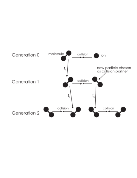
Figure 2: The collisional cascade system. Each “generation” involves a single collision for all particles in the system. The collision partners for these particles are selected statistically, as described in the text. The t_is are the times between collisions.

For practical reasons these simulations must avoid having to track large numbers of particles through space with a precision great enough to determine collisional impact parameters for molecular collisions. Thus the only information which can be used to determine collisions is the relative velocities of all the molecules and the system density. A total collisional cross–section allows selection of collision partners, as detailed below, while partial cross–sections for deflection angle and internal (de)excitation allow the outcome of the resulting collisions to be determined.

Collision times and partners are selected by the following process. Consider two particles, $i$ and $j$, in a box with repeating boundary conditions. The average time for particle $i$ to collide with particle $j$ is given by $t_{ij}=1/\rho_{j}\sigma v_{ij}$ where $\rho_{j}$ is the number density of particle $j$, $\sigma$ is the total collisional cross–section and $v_{ij}$ is the relative velocity of $i$ and $j$. The time to an actual collision is given by $\tau_{ij}=t_{ij}R$, where $R$ is an exponentially distributed random variable centered on 1. If there are many particles in the box then the time until the next collision that particle $i$ undergoes, $\tau_{i}$, is $\min_{j}\tau_{ij}$. In a full system this minimisation is taken over 10 potential collision partners selected from a population with the correct velocity distribution (taken to be Maxwellian at a specified temperature). For the purposes of calculating the times each is taken to have a number density on tenth that of the local medium. This procedure has been shown to give the correct relative velocity distribution function and collision time distribution over a sufficient number of collisions for a non–radiating, thermal gas, the only system for which such distributions are well–known.

When a collision partner has been selected its internal state is calculated. For low–temperature systems the internal states are taken to be initially thermal at the kinetic temperature. At higher temperatures this may not be a good assumption, due to depletion in any unexcited gas due to long collisional reexcitation times (Chang & Martin 1991, for example) or residual excitation from previous high–energy collisional cascades. The initial population is not critical, however, as the non–thermal populations are much higher for ion velocities in excess of 10 kms^-1. In simulations of entire shocks the evolution of these states may be important. An ortho–para ratio of 3 is used throughout, and there are no ortho–para conversion mechanisms included in the simulation.

In order to determine the effects of heating a large body of gas over a wide temperature range a series of cascades is necessary, incorporated into a complete dynamical shock model. While this is not yet possible using this model the likely properties of such a system are indicated in the short chains of cascades that have been calculated.

5 Results

There is a strong non–thermal character both to the radiation and residual excitation resulting from collisional cascades. Rapid excitation to high–energy internal states in the first few collisional generations, when the non–thermal energies are highest, is followed by gradual deexcitation due both to collisional and spontaneous deexcitation. The population changes over time are indicated in figure 3. The shorter radiative deexcitation times of, and existence of multiple decay paths for, more highly excited states means that they decay more rapidly, although the logarithmic scale on the y–axis tends to disguise this. As the excitation energy for H₂ is so high (the lowest excitation is at 510K) most molecules will initially be in the ground state of ortho– or para–H₂ (V=0, J=1,0) at the temperatures considered. Combined with the excitation cutoff at $J\rightarrow J+6$, this means that the populations of states with $J>7$ are lower than their energy would suggest, as they require multiple collisions to become populated. However, even within a ten generation cascade a significant number of particles can undergo multiple collisional excitations.

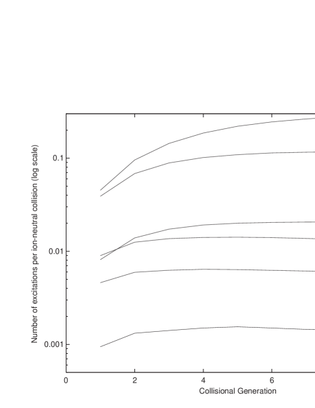
Figure 3: The evolution of population with cascade generation for a selection of internal states for a system with T=500K, $\rho=10^{4}{\rm cm}^{-3}$ and v${}_{\rm in}=15{\rm kms}^{-1}$, typical of the early stages of a MHD shock. There are no excitations in the 0th generation, the ion–neutral collision. Initial collisional excitation of high energy states is followed by collisional and radiative depopulation, though at these densities a large proportion of the excitations are still present after 10 generations.

The most important result of these simulations is the relative populations of the various internal states of H₂ as derived from radiation from the system. Figure 4 shows these populations for a system with parameters typical of the ambipolar region of a MHD shock, relative to the expected populations for a thermal gas at 2000K. This is so that the plot may be directly compared with those in, for example, Brand et al. 1988 and Richter et al. 1995. The population is plotted against the energy of the upper level, in 1000K, and a logarithmic scale is used on the y axis. The absolute scale on the y–axis will vary with the proportion of molecules involved in cascades. This graph assumes that all particles are in cascades, corresponding to an ionisation fraction of roughly 10^-6.

Any straight line on this plot would indicate a gas at a single temperature, so it is clear that no single temperature can explain all these data, in marked contrast with previous magnetic shock models. Instead, the excitation temperature of the internal states shows a strong trend to increase with increasing level energy, agreement with observed H₂ shocks in OMC–1 and IC443, previously explained using complex multi–component shocks or cooling zones following partially–dissociative shocks. The errors shown are $\sqrt{N}$ only. As the absolute relative populations of the higher energy states are very low, albeit much higher than for thermal systems, reducing the errors in these populations is very expensive computationally.

Figure 4: The relative populations of internal states of H₂, as derived from the cascade radiation, for the system in figure 3. The populations are shown relative to those expected for a thermal system at 2000K, following Brand et al. 1988. Different V sequences are differentiated to show that the energy of the level is the main factor determining the relative population, in line with observations. Error bars are formal only.

The shape of the curve in figure 4 is a function of the neutral kinetic temperature, ion–neutral streaming velocity (v_in) and neutral particle density, as described below.

• Neutral Kinetic Temperature: As the initial neutral internal populations are taken to be those for a thermal system the temperature determines the emission from the thermal lines, and has a small effect on those states which are not thermally populated.

• Ion–Neutral Streaming Velocity: As this determines the amount of non–thermal energy available in a given cascade it also governs the number of non–thermal excitations which occur and their energy range. Below v${}_{\rm in}\simeq 10{\rm kms}^{-1}$ there are negligable levels of internal excitation, but above this they increase strongly with v_in.

• Density: At low densities most excitations will lead to radiation whereas collisional deexcitation becomes dominant at higher densities. There appears to be a critical density above which the radiation from a cascade is essentially invariant for a few orders of magnitude in density, as shown in figure 5. This critical density is just below the densities predicted for the H₂ shock in OMC–1 (Brand et al. 1988).

Figure 5: Derived level populations against level energy for a range of densities for a system at 500K with v_in=15kms^-1. The emission appears to be independent of density above $\rho=10^{4}{\rm cm}^{-3}$.

Using these calculations to model an entire shock is not yet possible, chiefly due to computational constraints. The effects of residual enhancements in population levels following cascades can be seen, however, in calculations where these populations are used as the input to subsequent cascades. After a series of such cascades it is clear that this enhancement does occur, even for relatively low densities, as illustrated in figure 6. Due to these increased internal populations later runs also have enhanced radiation from higher energy states. At each stage the kinetic temperature increases as indicated, while the rotational and vibrational populations increase more rapidly. The effect is seen most strongly at higher energies, where the residual populations are several orders of magnitude higher than would be seen in a thermal gas. These states cannot easily be excited from the ground state, and the residual excitation populations enable them to be populated.

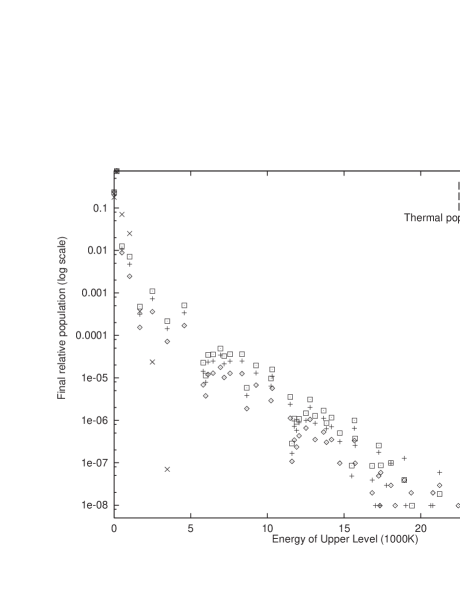
Figure 6: Residual internal states after cascade simulations. Here the final populations and kinetic temperature from iteration 1 are used as the inputs for iteration 2, and so on. v_in=15 kms^-1, $\rho$=10⁴cm^-3 in all runs. There is a definate buildup of populations of higher energy states, well in excess of the corresponding increase in kinetic temperature.

The observed internal populations, which are an unavoidable result of the process of ambipolar diffusion, are strongly reminiscent of those which have been observed in H₂ shocks in OMC–1 and IC443, where the excitation temperature is also an increasing function of level energy and is almost independent of the details of V and J state. There are two major differences between the data sets. The first is the absolute magnitude of the radiation, which is higher for observed systems than in the data presented here. For observations this scale will depend on assumptions about the system density. For this model it will vary with the ratio of ion–neutral collisions to pure neutral ones and, therefore, with the ionisation fraction. The scales shown assume an ionisation fraction of approximately 10^-6. The second major difference is the behaviour of the populations above about 15000K. These have been observed by Brand et al. (1988) and Richter et al. (1995) to rise dramatically whereas these calculations show, at best, a modest increase. This is probably due to the conservative nature of the extrapolations and the arbitrary excitation cutoff at J$\rightarrow$J+6, both of which limit the populations of highly excited states, as well as the differential cross–sections used, which disperse energy extremely efficiently and thus serve to reduce the population of very high velocity particles rapidly.

6 Further Work Needed

The main difficulty with applying these calculations is the uncertain and unreliable nature of both differential and internal excitation rate coefficients. This work shows the importance of high–quality quantum mechanical calculations of these coefficients if H₂ line ratios are to be used as diagnostics in molecular clouds.

A calculation of the integrated emission from a complete shock is needed to test the importance of these results both for the dynamics of shocks and the resulting molecular line ratios. Such a calculation will be computationally expensive. Simple order–of–magnitude calculations show that the line strengths in figure 4 correspond to those which would be observed from a magnetic shock travelling at 25 km s^-1 through a medium with $\rho\sim 10^{4}{\rm cm}^{-3}$ and $10^{-7}\leq{\rm x}_{i}\leq 10^{-4}$, typical conditions in these regions. The first few ($<$1000K) states will also have a significant contribution from thermal emission for ionisation fractions of this order.

7 Conclusions

Non–LTE excitation populations in H₂ are a natural consequence of ambipolar diffusion in molecular shocks, with no need for complex geometrical constructions or multicomponent shock models. Comparison of figure 4 with observations in Brand et al. (1988), for example, show that this mechanism could explain the observed line ratios in OMC–1 and IC443, with the reservation that the poor quality of available cross–sections does not allow firm predictions to be made. The conservative nature of these calculations mean that the upturn in excitation populations which have been seen observationally at higher energies could result from this process also. Full shock models incorporating this theory are possible and should be carried out to determine the integrated emission over whole shock regions.

References

Brand, P.W.J.L., Moorhouse, A., Burton, M.G., Geballe, T.R., Bird, M. and Wade, R., 1988, Ap. J., 334, L103

Buck, U., Huisken, F., Kohlhase, A., Otten, D., 1983a, J. Chem. Phys, 78, 4439

Buck, U., Huisken, F., Maneke, G., 1983b, J. Chem. Phys, 78, 4430

Chang, C.A., Martin, P.G., 1991, Ap. J., 378, 202

Danby, G., Flower, D.R., Montiero, T.S., 1987 M.N.R.A.S., 226,739

de Jong, T., Dalgarno, A., Boland, W., 1980, Astr. Ap.. 91, 68

Dove, J.E. and Teitelbaum, H., 1974, Chem. Phys., 6, 431

Draine, B.T., 1980, Ap. J., 241, 1021

Draine, B.T., McKee, C.F., 1993, Ann. Rev. Astron. Astrophys., 373-432

Draine, B.T., Roberge, W.G., Dalgarno, A., 1983, Ap. J., 264, 485

Lepp, S., Schull, J.M., 1983, Ap. J., 270, 578

McKee, C.F., Chernoff, D.F., Hollenbach, D.J., 1984, in Galactic and Extragalactic Infrared Spectroscopy, ed. Kessler, M.F., Phillips, J.P., 103, Dordrecht: Reidel

Richter, M.J., Graham, J.R., Wright, 1995a, Ap. J., submitted

O’Brien, I.T., 1995, PhD Thesis

Smith, M.D., 1991, M.N.R.A.S., 253, 175