Retention Fractions for Globular Cluster Neutron Stars

Abstract

Fokker-Planck models are used to give estimates for the retention fractions for newly-born neutron stars in globular clusters as a function of kick velocity. These can be used to calculate the present day numbers of neutron stars in globular clusters and in addressing questions such as the origin of millisecond pulsars. As an example, the Population I kick velocity distribution of Lyne & Lorimer [1994] is used to estimate the retained fractions of neutron stars originating as single stars and in binary systems. For plausible initial conditions fewer than 4% of single neutron stars are retained. The retention fractions from binary systems can be 2 to 5 times higher. The dominant source of retained neutron stars is found to be through binary systems which remain bound after the first supernova, ie. high-mass X-ray binaries. The retained fraction decreases with an increasing number of progenitors, but the retention fraction decreases more slowly than the number of progenitors increases. On balance, more progenitors give more neutron stars in the cluster.

1 Introduction

Globular clusters are now known to contain a population of neutron stars. There are 34 pulsars observed in globular clusters, 30 of them of the millisecond variety [1995], and 12 low-mass x-ray binaries (LMXBs) [1993] which probably contain neutron stars.

The generally accepted scenario for neutron star formation and evolution gives their origin in Type II supernovae and for them to slowly spin down. The millisecond pulsars are thought to be the result of recycling by accretion of matter from binary companions. For globular clusters, as well is in the Galaxy at large, this picture has been the matter of some controversy. The presumed progenitors of the millisecond pulsars are the LMXBs, but some (see for example Bailyn & Grindlay 1990) feel that this is inconsistent with the relative numbers of the two objects.Rather than being spun-up neutron stars, the millisecond pulsars would, in this picture, come from the accretion induced collapse of a white dwarf pushed over the Chandrasekhar limit. (See the review of Bhattacharya & van den Heuvel 1991 for a thorough discussion of these issues.) One of the key issues in this debate is the rate at which stellar interactions cause neutron stars to end up in binary systems leading to mass transfer and being spun up. An essential ingredient in estimating this is the total number of neutron stars present in the system.

Lyne & Lorimer [1994] have recently reevaluated the distribution of space velocities of young field pulsars. Based on their sample the mean birth, or “kick”, velocity of neutron stars is 450 km s^-1. The typical escape velocity of a globular cluster is of order 20 km s^-1, so if the globular cluster neutron stars are born with similar velocities, we would expect very few to remain in the clusters.

Verbunt & Hut [1987] attempted to estimate a global retention fraction for globular cluster neutron stars. They assumed a typical escape velocity of 30 km s^-1 and used the lower kick velocity distribution of Lyne, Anderson, & Salter [1982]. They estimated the retention fraction be $\sim 0.15$. This treatment was updated by Hut, Murphy, & Verbunt [1991] who used a collision-weighted average escape velocity of 47.7 km s^-1 and estimated the retention fraction to be 0.3. These estimates are unsatisfactory since they are based on a single escape velocity and do not account properly for the variation in escape velocity within each cluster and between clusters. There is a need for a more realistic treatment of neutron star retention using dynamical models of globular clusters. This is all the more necessary in view of the increase in the mean kick velocity in Lyne & Lorimer [1994].

The aim of this paper is to provide curves giving retention fractions as a function of kick velocity for a series of dynamical Fokker-Planck models. These are presented in the next section. As an example of their use, in §3 I will calculate the overall retention rates for single stars assuming the Lyne & Lorimer [1994] velocity distribution, and the retention rates of binary fragments using the results of Brandt & Podsiadlowski [1995].

2 Retention Fractions

Consider a star with velocity $v$ at a position in the cluster where the escape velocity is $v_{e}$ which receives a velocity kick $v_{k}$. We assume that both velocities are isotropically distributed so that the angle $\theta$ between them is distributed as

$$P(\theta)={1\over 2}\sin\theta.$$ (1)

The resultant velocity, $v_{r}$, is

$$v_{r}=\sqrt{v^{2}+v_{k}^{2}+2vv_{k}\cos\theta}.$$ (2)

The star will remain bound to the cluster provided that $v_{r}<v_{e}$, ie. so long as

$$\cos\theta<\cos\theta_{e}\equiv{v_{e}^{2}-(v^{2}+v_{k}^{2})\over 2vv_{k}}.$$ (3)

The probability that the star will be retained by the cluster is

$$P({\rm ret}|v,v_{k},v_{e}) = \int_{\theta_{e}}^{\pi}P(\theta)d\theta$$ (4)

$$= {\cases{1,&${v_{k}\over v_{e}}-1\leq-{v\over v_{e}}$;\cr{1-({v-v_{k}\over v_{e}})^{2}\over{4vv_{k}\over v_{e}^{2}}},&$\left|{v_{k}\over v_{e}}-1\right|<{v\over v_{e}}$;\cr 0,&${v_{k}\over v_{e}}-1\geq{v\over v_{e}}$.\cr}}$$

Note that $v_{k}$ and $v$ in eq. (4) can be written in terms of $v_{e}$, so let $\hat{v}=v/v_{e}$ and $\hat{v}_{k}=v_{k}/v_{e}$ and then

$$P({\rm ret}|\hat{v},\hat{v}_{k})={\cases{1,&$\hat{v}_{k}-1\leq-\hat{v}$;\cr{1-(\hat{v}-\hat{v}_{k})^{2}\over 4\hat{v}\hat{v}_{k}},&$\left|\hat{v}_{k}-1\right|<\hat{v}$;\cr 0,&$\hat{v}_{k}-1\geq\hat{v}$.\cr}}$$ (5)

If $\hat{v}_{k}>1$, then all stars with $v<v_{k}-v_{e}$ will escape from the cluster, while if $\hat{v}_{k}<1$, then all stars with $v<v_{e}-v_{k}$ are retained. All stars escape if $\hat{v}_{k}>2$.

In order to get the total retention probability as a function of $v_{k}$ for a given star system, we need the number of stars as a function both of position and velocity. For the purposes of this calculation, I assume a spherically symmetric cluster with an isotropic velocity dispersion. The distribution function is then a function of the energy alone. The density and potential can be derived from the distribution function, as can the velocity distribution at each radius.

In general, for a known distribution function, $f(r,v)$, the number of stars retained at radius $r$ as a function of $\hat{v}_{k}$ is

$$N_{\rm ret}(r,\hat{v}_{k})=4\pi\int_{0}^{1}P({\rm ret.}|\hat{v},\hat{v}_{k})\hat{v}^{2}f(r,\hat{v})d\hat{v}.$$ (6)

Using eq.(5),

$$N_{\rm ret}(r,\hat{v}_{k}) = H(1-\hat{v}_{k})4\pi\int_{0}^{1-\hat{v}_{k}}\hat{v}^{2}f(r,\hat{v})d\hat{v}$$ (7)

$$+{\pi\over\hat{v}_{k}}\int_{1-\hat{v}_{k}}^{1}{\hat{v}}(1-(\hat{v}-\hat{v}_{k})^{2})f(r,\hat{v})d\hat{v},$$

where $H(x)$ is the Heaviside unit function. For a distribution function in energy $f(E)$, as is appropriate for the isotropic, spherically symmetric models to be discussed below, we can rewrite the number retained as

$$N_{\rm ret}(r,\hat{v}_{k}) = {4\pi\over\left(2\left|\phi(r)\right|\right)^{3\over 2}}\left[H(1-\hat{v}_{k})\int_{l}^{1\over 2}\left(1-2A\right)^{1\over 2}f\left({A}\right)dA\right.$$ (8)

$$+{1\over 2\hat{v}_{k}}\int_{0}^{l}Af\left({A}\right)dA$$

$$+{1\over 2}\int_{0}^{l}\left(1-2A\right)^{1\over 2}f\left({A}\right)dA$$

$$\left.-{\hat{v}_{k}\over 4}\int_{0}^{l}f\left({A}\right)dA\right].$$

The energy has been normalized by the local escape velocity so $E=2\phi(r)A$, where the potential goes to zero at infinity. The limit on the integration is given by $l=\hat{v}_{k}(2-\hat{v}_{k})/2$ and is a function of radius since $\hat{v}_{k}$ depends on the local escape velocity. Equation (8) can then be integrated over all radii and divided by the total number of stars to give the total fraction of stars retained as a function of $v_{k}$, $f_{\rm ret}(v_{k})$.

The approach taken here was to evaluate the total fraction of stars retained using Monte Carlo techniques. To begin with, I consider the isotropic, single-mass, Michie-King models [1966]. These form a single parameter family in terms of their degree of central concentration. The parameter is often given as the dimensionless central potential $W_{0}$. For a series of models in this family, the density distribution and potential were calculated. For each test value of $\hat{v}_{k}$ (the models are dimensionless and the local escape velocity scales with the central escape velocity $v_{e_{c}}$), stellar positions were drawn at random with a distribution consistent with the radial number density. For each position, the velocity distribution was computed from the lowered-Maxwellian distribution function. The relative angle between the velocity vectors was chosen at random from the distribution in eq. (1) and the $v_{r}$ was computed. The retention fraction for the chosen $\hat{v}_{k}$ is then the ratio of test stars with $v_{r}<v_{e}(r)$ to the total number of test stars. Sufficiently large samples were used to ensure numerical precision.

Figure 1 shows the retention fractions as a function of $v_{k}/v_{e_{c}}$, $v_{e_{c}}$ is the central escape velocity, for a range of Michie-King models. The retention fractions are tabulated in Table 1 Note that the lower concentration models are most able to retain their neutron stars for a given $v_{k}/v_{e_{c}}$ since they have a greater number of stars within their cores. On the other hand, a low concentration model must have a much higher mass than a high concentration model to have the same central escape velocity. This scales as $\sqrt{M/r}$ where $M$ is the total mass of the system and $r$ is some scale radius.

In order to make more realistic estimates of the retention fractions, I have done similar Monte-Carlo integrations of eq. (8) for a series of Fokker-Planck models. These models are as described in Drukier [1995] with the differences discussed here. The models are based on direct numerical integration of the orbit-averaged form of the Fokker-Planck equation following the technique of Cohn [1980]. A mass spectrum is included as are the effects of stellar evolution. Since only the early time evolution of the models is required, the tidal stripping and binary heating as described in Drukier [1995] have been turned off. Stellar evolution has been handled by having each bin evolve over a time interval corresponding to the lifetimes of stars at the bin boundaries. Since even the most massive stars take time to complete their evolution, the earliest stages of the evolution of the models are governed by two-body relaxation alone. Dynamical friction can lead to a large degree of initial mass segregation when stellar mass-loss and neutron star formation commences.

The treatment of stellar evolution has been modified from that described in Drukier [1995] by adding an auxiliary mass species to hold the distribution function for the remnants as they evolve. At each time step an appropriate fraction of the progenitor distribution function is transferred to the remnants. The mean mass of the two bins still changes linearly over the time interval for evolution, but each of the two populations of stars, with their very different masses, are free to evolve separately. At the same time as the transfer is done at each time step, the transferred distribution function and its associated density profile are saved, together with the current potential. These are then used in the integration of eq. (8) at that time step. An appropriately weighted sum is computed to give the overall retention fraction for the model cluster.

The mass range adopted for these models is from 32 $M_{\mathord{\odot}}$to 0.1 $M_{\mathord{\odot}}$. Neutron star progenitors are assumed to have masses above 8 $M_{\mathord{\odot}}$. It is likely that in Population II stars with masses as low as 5 $M_{\mathord{\odot}}$will give rise to supernovae, but whether they leave a remnant or not is unknown [1993]. For such a large mass ratio, dynamical friction can be an important effect. I have used four logarithmically spaced bins for the neutron stars in these models. Tests using only one or two bins gave substantially the same results, as did models with a lower mass limit of 0.15$M_{\mathord{\odot}}$.

The models are assumed to start as Michie-King models with $W_{0}=3$, 5, or 7; initial mass $M=10^{5}$, $5\times 10^{5}$, $10^{6}$, or $5\times 10^{6}$ $M_{\mathord{\odot}}$; and limiting radii $r_{l}$ between 15 and 65 pc with one model at 97 pc. The grid was not fully sampled. The initial mass function (IMF) is assumed to take the form of a power-law

$$N(m)\,dm\propto m^{-(x+1)}\,dm,$$ (9)

with mass-spectral-index $x$; $x=1.35$ for the Salpeter mass function. Models with $x=1$ and $x=2$ were run. For $x>2$ there are very few massive stars in the cluster to begin with.

The initial parameters of the models run are listed in Table 2 and Table 3 sorted by initial half-mass relaxation time. The tables give the run identification number; the model parameters $W_{0}$, $r_{l}$, $x$, and $M$; the half-mass relaxation time [1981]; and the number of neutron-star progenitors. Only the models with relaxation times less than 20 Gyr have been included. For the models listed in Table 2, the retention fractions as a function of $v_{k}$ are listed in Table 4. The table columns are arranged by model number, and give the retention fractions for a range of velocities. The corresponding velocity in km s^-1 is the index number of the retention fraction multiplied by the number under the model number. I have listed the initial parameters of the models in Table 3 for completeness. These models retain none of their neutron stars. Their escape velocities are less than about 8 km s^-1 so that all neutron stars born with velocities greater than about 15 km s^-1 escape.

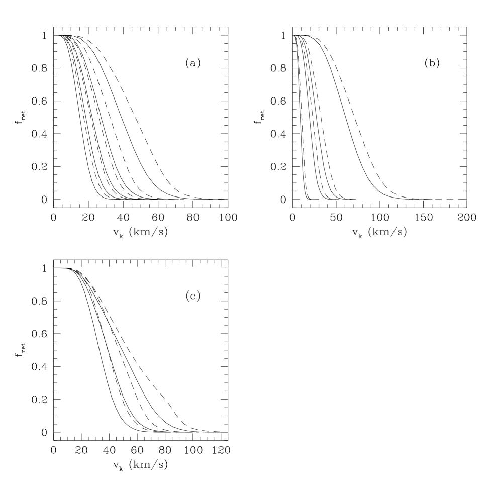
Figure 2: These figures show the effect on the retention fractions of varying the initial model parameters. All the panels show the retention fraction as a function of kick velocity for a range of models differing in only one parameter. Solid lines are for $x=1$ and dotted lines are for $x=2$. Note that at a given $v_{k}$, the $x=2$ models retain a higher fraction than do the $x=1$ models. (a) The models all have $M=10^{6}M_{\mathord{\odot}}$ and $W_{0}=5$. The retention fraction decreases with increasing model size as defined by $r_{l}$. In order of increasing $v_{k}$ at constant $f_{\rm ret}$, $r_{l}=97$, 65, 45, 30, and 15 pc. (b) The models all have $r_{l}=30$ pc and $W_{0}=5$. The retention fraction increases with increasing mass. In order of increasing $v_{k}$ at constant $f_{\rm ret}$, $M=10^{5}$, $5\times 10^{5}$, $10^{6}$, and $5\times 10^{6}$ $M_{\mathord{\odot}}$. (c) The models all have $r_{l}=15$ pc and $M=10^{6}M_{\mathord{\odot}}$. The retention fraction increases with increasing concentration. In order of increasing $v_{k}$ at constant $f_{\rm ret}$, $W_{0}=3$, 5, and 7.

The effects on the retention fraction of varying the model parameters are shown in Fig. 2. At a given value of $v_{k}$ the fraction retained increases with decreasing cluster size, increasing mass and increasing concentration. Models with smaller sizes, larger masses, or higher concentrations have larger escape velocities and can thus retain a higher fraction of stars at a given velocity. The variation with $r_{l}$ and $M$ are comparable, but $M$ has a much larger range in globular clusters. The variation with concentration is much the same as for the Michie-King models in Figure 1 when proper attention is paid to the scaling.

For all values of $v_{k}$, the models with $x=2$ have a higher $f_{ret}$ than the corresponding models with $x=1$. Since the $x=2$ models have fewer massive stars than the $x=1$ models, they lose less mass during the supernovae. Hence, the mean escape velocity over the period of massive star evolution is higher for the $x=2$ models and more neutron stars are retained. The difference with $x$ is fairly small and the additional retention fraction is tightly connected with a lower number of neutron-star progenitors. The net result is that the total number of neutron stars in an $x=2$ cluster will be lower than in an $x=1$ cluster.

Although it is not obvious from Figure 2, apart from a velocity scale factor the retention curves for each $x$ and $W_{0}$ are very similar. Further, they are quite similar to curves for the appropriate $W_{0}$ in Figure 1. To test this, I have compared the retention fraction curves with the curves for the appropriate Michie-King models. I have fit a scale velocity between the two curves and then computed the absolute maximum difference in $f_{ret}$. For $x=1$ the maximum difference is 0.03 for model 1 and for $x=2$ the maximum difference is 0.05 for model 3. The size of the maximum difference generally decreases with increasing $t_{rh}$, but the relationship is a complicated combination of the structural parameters $W_{0}$, $r_{l}$, and $M$.

On the other hand, we can estimate the scaling velocity from the parameters as

$$v_{e_{c}}=v_{e}(W_{0})\sqrt{f_{M}M/r_{l}},$$ (10)

where $f_{M}$ is the fraction of the total mass remaining after the end of neutron star formation and is 0.776 for $x=1$ and 0.991 for $x=2$. Values for $v_{e}(W_{0})$ are given in Table 5 for $M$ in $M_{\mathord{\odot}}$ and $r_{l}$ in pc. (The King [1966] concentration parameter $c=\log(r_{l}/r_{c})$ has also been listed for those unfamiliar with $W_{0}$.) This value of the scale velocity is within a few percent of the best fit estimate, but decreases with respect to the best fit value as the relaxation time decreases. Another way to look at this is that for short relaxation times, retention fractions calculated using the parameter estimate of the scale velocity and the Michie-King retention curves are systematically smaller than the retention fractions from the Fokker-Planck models themselves. This can be attributed to dynamical friction which enhances the number of neutron-star progenitors in regions with large escape velocities. The limited amount of two-body relaxation which takes place before stellar evolution mass loss begins also enhances the central potential and the neutron star retention rate. There is a small difference in the shape of the curves for $x=2$ and $W_{0}=7$ for short relaxation times. This is clearly due to mass segregation from dynamical friction. This limits the accuracy of the approximation. The maximum absolute difference in the retention fractions are 0.12 for $x=2$ and $0.08$ for $x=1$.

Bearing in mind these systematic differences, we can approximate a retention fraction curve for models unlike those given in Table 2 by using the appropriately scaled retention curves from Table 1. The effect of this approximation on the final retention rates will depend on the kick velocity distribution employed. A feeling for the size of the uncertainty can be taken from comparisons of rates based on Table 4 curves with rates based on scaled Table 1 curves.

3 Use of the retention fractions

Once $f_{\rm ret}(v_{k})$ is available, we can calculate the retention fraction of neutron stars in a given model by assuming a distribution of kick velocities. Here, I use the distribution estimated by Lyne & Lorimer [1994] for the Population I pulsars. Note that the correct value of the parameter $m$ is 0.3, not 0.13 as published (D. Lorimer, private communication). The results for a range of models are listed in the column labelled $f^{s}_{r}$ in Table 6. For the most part, less than 1% of the neutron stars are retained by the models. Only models with initial masses of $5\times 10^{6}M_{\mathord{\odot}}$ retain more than 3% of their initial neutron stars. In no case does a model retain more than 10%. I have also tried models with a larger range of neutron star progenitors. This only changes the retention fractions by 10% or so, but such a model would have a larger number of neutron stars to retain.

The number of neutron stars retained for each model, under the assumption that all the progenitors were single stars, is listed in the column labelled $N^{s}_{NS}$ in Table 6. Only models with $x=1$, $M=5\times 10^{6}M_{\mathord{\odot}}$ and either highly concentrated (high $W_{0}$) or compact (small $r_{l}$) retain more than 1000 neutron stars in this scenario. For less massive models, the maximum number of retained neutron stars is of order 100 for $x=1$ and of order 10 for $x=2$. Clearly, under these assumptions, very few neutron stars would be retained in most globular clusters.

Until now, I have assumed that the neutron star progenitors are single stars. Most massive stars, however, are members of multiple star systems, and the effects of multiplicity on the neutron star retention rates must be included. There are three possible outcomes when the primary star in the binary becomes a supernova and receives its kick. The system may become unbound, the system may remain bound with a change in its center-of-mass velocity, or the neutron star may pass close to the companion, or even hit it in the extreme case, triggering mass transfer and probable merger, forming a Thorne-Żytkow object. Brandt and Podsiadlowski [1995] used the same Lyne & Lorimer [1994] velocity spectrum to calculate the relative proportions of each outcome and the velocity distribution of the resulting binaries.

I have used the results for the high-mass x-ray binaries from section 3.2 of Brandt and Podsiadlowski [1995]. This work was meant as an exploratory investigation, so they used only one set of initial masses, but a distribution of initial periods. The calculations were based on a set of plausible, but arbitrary assumptions with regard to mass transfer in the evolving binary. As in Brandt and Podsiadlowski, the estimates given here are intended as suggestive rather than definitive.

Although not explicitly given in Brandt and Podsiadlowski [1995], the same calculation can also give the resulting velocities for each of the components of a disrupted system and for the merged remnant of the TŻO. The velocity distributions for the four types of results, assuming the Lyne & Lorimer [1994] kick distribution, are show in Figure 3. The upper panel shows the distribution of speeds for the low velocity products: the former companion in the unbound systems, the centre-of-mass motion of the bound binaries, and the motion of the merged objects. The bi-modal distribution of speeds for the unbound companion is a result of the two possible masses of the star under the two different regimes of stable or dynamical mass transfer (see Brandt and Podsiadlowski 1995 for details). The velocity distribution for the new-born, unbound neutron stars is given in the lower panel. It has the same peak as the Lyne & Lorimer [1994] velocities, but a longer high-velocity tail. In passing, this may suggest that the high-velocity pulsars in the Lyne & Lorimer sample may have their origin in binaries and that the true kick-velocity distribution truncates at lower velocities. If this were the case, the neutron star retention fraction would be somewhat increased, but since the mode of the distributions remains at around 250 km s^-2, it would not be a large effect.

For each channel of evolution, we can calculate the overall probability of retention using the curves as from Table 4. For a disrupted system, the overall retention fraction is calculated using the velocity distributions for the freed neutron star and its former companion. The companion, if retained by the cluster, is assumed, by two-body interactions, to rejoin the general background distribution of velocities. (Dynamical friction is a quick process.) Its retention probability in its subsequent supernova is given by the single star retention rate. The retention fraction of stars in the TŻO channel is also calculated using their distribution of resultant velocities.

For the systems which remain bound, the distribution of changes in center-of-mass velocity based on Brandt and Podsiadlowski [1995] is used for the distribution of kick velocities. The subsequent evolution of these systems is highly dependent on their new orbital parameters and the environment, but somewhere between 0 and 2 neutron stars remain bound to the cluster from each system. Systems with sufficiently short periods are expected to become high-mass X-ray binaries and experience a spiral-in phase resulting in the formation of a TŻO. The envelope will then be ejected leaving a single neutron star bound to the cluster, no second supernova having occured. Systems with longer periods will probably suffer a common-envelope phase and leave a short-period binary consisting of a helium star and a neutron star. Such systems would have a second supernova [1991]. The critical period is somewhere around 100 days [1978] and the majority of the systems in Brandt & Podsiadlowski [1995] had periods less than 100 days. On the other hand, their Figure 8b shows that there is a correlation between centre-of-mass velocity and period in the sense that the longer period systems had lower centre-of-mass velocities and thus were more likely to be bound to the cluster. Overall, it is plausible that each initial binary results in a single neutron star remaining in the cluster.

Given the fractions from each channel, the total fraction of neutron stars originating in binaries which are retained by the cluster is given by

$$f_{r}^{\rm bin}(a)=(1-f_{b})(f_{r}^{u1}+f_{r}^{s}f_{r}^{u2})+f_{b}(f_{t}f_{r}^{t}+(1-f_{t})af_{r}^{b}),$$ (11)

where $f_{b}$ is the fraction of systems which remain bound, $f_{t}$ is the fraction of the bound systems becoming TŻOs (the fraction of unbound systems which suffer close encounters as the neutron star escapes is very small), and the factors subscripted $r$ are the retention fractions for the various populations: $f_{r}^{u1}$ for the unbound neutron stars, $f_{r}^{u2}$ for their former companions, $f_{r}^{s}$ for the single neutron stars as above, $f_{r}^{t}$ for the TŻOs, and $f_{r}^{b}$ for the systems which remain bound. The factor $a$ deals with the fate of the binary systems. Its value lies between 0 and 2, but is likely to be 1 as discussed above. For the models listed in Table 2, I list in Table 6 the retention fractions for the various processes. I have taken $f_{b}=0.27$ and $f_{t}=0.26$ based on Brandt & Podsiadlowski [1995], but it should be noted that these came from a particular set of assumptions and initial conditions and should be considered as approximate. The first column gives the model number as in Table 2, the next five columns give fraction of neutron stars retained through each individual channel listed above. The next two columns give the combined fraction retained from the binary systems using eq.(11) and assuming that $a=0$ or 2. The next column gives the number of neutron stars retained if they are all single stars and the final three columns give the expected number of retained neutron stars under the assumption that all the neutron star progenitors are in binary systems, but that either the bound binaries leave no neutron stars in the cluster (the $a=0$ case), $N_{NS}^{b}(0)$, that they leave one neutron star (the $a=1$ case), $N_{NS}^{b}(1)$, or that they leave two neutron stars in the cluster (the $a=2$ case), $N_{NS}^{b}(2)$. The $a=1$ case gives the most likely value.

By comparing the $f_{r}^{s}$ column and the two $f_{r}^{\rm bin}$ columns, it is clear that neutron stars originating from binaries are more likely to be retained than neutron stars from single stars. Further, the major mechanism for retaining neutron stars is through the channel of binaries which remain bound and binary after the first supernova. If the fate of these systems is as discussed above, then these binaries will ultimately leave one neutron star without any further violent events to eject it from the cluster. Thus, on the assumptions made here, most globular cluster neutron stars will have passed through a high-mass X-ray binary phase.

Between clusters, it is also clear from Table 6 that the shape of the initial mass function will play a crucial role in determining the number of neutron stars in the cluster. The variation in the retention fractions with the mass function slope is relatively small, so of two clusters with the same structural parameters—initial mass, size, and concentration—the cluster with the larger number of massive stars will retain the larger number of neutron stars. This holds even if this cluster is somewhat less massive, less concentrated, or larger than the other cluster with the steeper initial mass function.

To illustrate this point further, and as an example of the use of the Michie-King model approximation, I estimate the number of retained neutron stars for two globular clusters. The main problem in making such estimates for particular globular clusters is that the initial conditions of the cluster are required, not the present state. Since the initial conditions are unknown, this presents a problem, but estimates can be made. I will consider two globular clusters: NGC 6397 and $\omega$ Cen. For NGC 6397, approximate initial conditions are known from the modelling in Drukier [1995]. The model used is model U30-B. Since the cluster had a fairly low initial mass, it is to be expected that it lost a large majority of its neutron stars. Drukier [1995] showed that some neutron stars had to have been retained, so I have taken the model with the largest initial number of massive stars. The $\omega$ Cen model assumes that the cluster hasn’t evolved very much, which is reasonable enough given its high mass and low concentration, but does include the appropriate change in the total mass. The parameters I adopt for the initial models are listed in Table 7. Table 7 also contains the estimates of the original and retained numbers of neutron stars under the same assumptions as in Table 6, except that for the number originating from binaries, $a=1$ is assumed. NGC 6397’s lower initial mass is balanced by its higher concentration, smaller size and larger number of neutron-star progenitors. $\omega$ Cen retains a much higher fraction of its neutron stars, but the two clusters end up retaining under the various scenarios the same numbers of neutron stars.

4 Conclusions

I have presented tables based on Fokker-Planck models which give the retention fractions of neutron stars as a function of the initial parameters of the models and of the neutron star kick velocity. I have also introduced an approximation technique using Michie-King models. These can be combined with a distribution of kick velocities to estimate the number of neutron stars retained by a globular cluster. One difficulty with this approach, is that the present structure of a globular cluster is not necessarily a good estimate of the state of the cluster when the neutron stars were formed.

These retention fractions have been integrated over the kick velocity distribution of Lyne & Lorimer [1994], and, as expected, very few single neutron stars are retained. The same distribution has been applied to the evolution of a model sample of high-mass binaries and the fraction of neutron stars retained from binaries was similarly estimated. Based on these estimates, the dominant source of globular cluster neutron stars would be via high-mass X-ray binaries. Both for neutron stars originating as single stars and in binaries, the number retained is strongly dependent on the number of neutron-star progenitors. Increasing the number of progenitors increases the total mass loss and reduces the fraction retained, but the larger number of stars more than makes up for this reductions.

The retention fractions given in this paper contribute only to the first stage in estimating the observed population of millisecond pulsars and LMXBs in globular clusters. The details of the rest of the evolution; i.e. how the neutron stars are spun up, is a matter for further study, but this paper should provide the tools to estimate the number of neutron stars the clusters have to work with.

Table 1: Retention fractions as a function of $v_{k}/v_{e_{c}}$ for Michie-King models

$v_{k}/v_{e_{c}}$	$W_{0}=1$	2	3	4	5	6	7	8	9	10	11
0.00	1.000	1.000	1.000	1.000	1.000	1.000	1.000	1.000	1.000	1.000	1.000
0.05	1.000	1.000	1.000	1.000	1.000	1.000	1.000	1.000	1.000	1.000	1.000
0.10	1.000	1.000	1.000	1.000	1.000	1.000	1.000	0.999	0.997	0.997	0.996
0.15	1.000	1.000	1.000	1.000	1.000	0.999	0.996	0.990	0.981	0.978	0.977
0.20	1.000	1.000	0.999	0.998	0.996	0.994	0.984	0.965	0.944	0.931	0.928
0.25	0.998	0.998	0.996	0.993	0.989	0.979	0.959	0.922	0.876	0.851	0.840
0.30	0.991	0.988	0.985	0.980	0.972	0.954	0.919	0.858	0.793	0.747	0.733
0.35	0.976	0.972	0.967	0.959	0.943	0.917	0.869	0.784	0.699	0.645	0.619
0.40	0.953	0.948	0.940	0.926	0.905	0.868	0.807	0.706	0.606	0.542	0.511
0.45	0.919	0.913	0.900	0.881	0.853	0.806	0.732	0.631	0.526	0.452	0.411
0.50	0.872	0.862	0.846	0.825	0.794	0.739	0.660	0.553	0.447	0.368	0.326
0.55	0.810	0.801	0.786	0.761	0.720	0.668	0.590	0.485	0.377	0.302	0.261
0.60	0.744	0.728	0.710	0.683	0.645	0.589	0.512	0.417	0.316	0.241	0.201
0.65	0.665	0.648	0.627	0.606	0.569	0.517	0.445	0.354	0.261	0.197	0.154
0.70	0.578	0.567	0.545	0.523	0.487	0.437	0.377	0.290	0.215	0.157	0.117
0.75	0.491	0.483	0.469	0.440	0.411	0.367	0.311	0.240	0.171	0.122	0.090
0.80	0.410	0.398	0.383	0.360	0.334	0.300	0.252	0.192	0.137	0.093	0.067
0.85	0.331	0.321	0.307	0.289	0.265	0.237	0.196	0.147	0.102	0.070	0.049
0.90	0.263	0.253	0.236	0.224	0.207	0.178	0.148	0.108	0.074	0.048	0.033
0.95	0.201	0.193	0.184	0.170	0.152	0.132	0.107	0.079	0.053	0.034	0.024
1.00	0.155	0.146	0.135	0.123	0.111	0.092	0.074	0.054	0.035	0.022	0.015
1.05	0.111	0.106	0.099	0.091	0.077	0.066	0.051	0.037	0.024	0.014	0.009
1.10	0.082	0.077	0.071	0.063	0.054	0.047	0.033	0.024	0.015	0.009	0.005
1.15	0.059	0.052	0.048	0.043	0.036	0.029	0.022	0.016	0.009	0.006	0.004
1.20	0.041	0.039	0.034	0.029	0.024	0.020	0.014	0.010	0.005	0.003	0.002
1.25	0.029	0.025	0.023	0.019	0.016	0.013	0.008	0.006	0.004	0.002	0.001
1.30	0.019	0.017	0.014	0.013	0.010	0.008	0.006	0.003	0.002	0.001	0.000
1.35	0.011	0.010	0.009	0.007	0.006	0.005	0.003	0.002	0.001	0.000
1.40	0.007	0.006	0.004	0.005	0.004	0.002	0.002	0.001	0.000
1.45	0.004	0.004	0.003	0.002	0.002	0.002	0.001	0.001
1.50	0.002	0.002	0.002	0.001	0.001	0.001	0.001	0.000
1.55	0.001	0.001	0.001	0.001	0.000	0.000	0.000
1.60	0.001	0.000	0.000	0.000
1.65	0.000

Table 2: Initial parameters for Fokker-Planck models

Run	$W_{0}$	$r_{l}$ (pc)	$M$ ($M_{\mathord{\odot}}$)	$x$	$t_{rh}$ (Gyr)	$N_{\hbox{\rm Massive}}$
1	7	15	$1\times 10^{5}$	1	0.26	1710
2	7	15	$5\times 10^{5}$	1	0.50	8550
3	5	15	$1\times 10^{5}$	1	0.53	1710
4	7	15	$1\times 10^{6}$	1	0.66	17100
5	7	15	$1\times 10^{5}$	2	0.68	80
6	5	15	$5\times 10^{5}$	1	1.03	8550
7	7	15	$5\times 10^{6}$	1	1.31	85500
8	7	15	$5\times 10^{5}$	2	1.33	402
9	5	15	$1\times 10^{6}$	1	1.37	17100
10	5	15	$1\times 10^{5}$	2	1.40	80
11	7	30	$5\times 10^{5}$	1	1.41	8550
12	3	15	$5\times 10^{5}$	1	1.76	8550
13	7	15	$1\times 10^{6}$	2	1.78	804
14	7	30	$1\times 10^{6}$	1	1.88	17100
15	7	30	$1\times 10^{5}$	2	1.92	80
16	3	15	$1\times 10^{6}$	1	2.35	17100
17	3	15	$1\times 10^{5}$	2	2.40	80
18	7	45	$5\times 10^{5}$	1	2.59	8550
19	5	15	$5\times 10^{6}$	1	2.71	85500
20	5	15	$5\times 10^{5}$	2	2.74	402
21	5	30	$5\times 10^{5}$	1	2.91	8550
22	7	45	$1\times 10^{6}$	1	3.45	17100
23	7	15	$5\times 10^{6}$	2	3.55	4020
24	5	15	$1\times 10^{6}$	2	3.67	804
25	7	30	$5\times 10^{6}$	1	3.72	85500
26	7	30	$5\times 10^{5}$	2	3.75	402
27	5	30	$1\times 10^{6}$	1	3.88	17100
28	7	60	$5\times 10^{5}$	1	3.98	8550
29	3	15	$5\times 10^{6}$	1	4.64	85500
30	3	15	$5\times 10^{5}$	2	4.69	402
31	3	30	$5\times 10^{5}$	1	4.97	8550
32	7	30	$1\times 10^{6}$	2	5.03	804
33	5	45	$5\times 10^{5}$	1	5.34	8550
34	7	65	$1\times 10^{6}$	1	5.99	17100
35	3	15	$1\times 10^{6}$	2	6.28	804
36	3	30	$1\times 10^{6}$	1	6.64	17100
37	7	45	$5\times 10^{6}$	1	6.83	85500
38	7	45	$5\times 10^{5}$	2	6.89	402
39	5	45	$1\times 10^{6}$	1	7.12	17100
40	5	15	$5\times 10^{6}$	2	7.32	4020
41	5	30	$5\times 10^{6}$	1	7.67	85500
42	5	30	$5\times 10^{5}$	2	7.74	402
43	5	60	$5\times 10^{5}$	1	8.22	8550
44	3	45	$5\times 10^{5}$	1	9.14	8550
45	7	45	$1\times 10^{6}$	2	9.24	804
46	7	30	$5\times 10^{6}$	2	10.04	4020
47	5	30	$1\times 10^{6}$	2	10.38	804
48	7	60	$5\times 10^{6}$	1	10.51	85500
49	7	97	$1\times 10^{6}$	1	10.93	17100
50	3	45	$1\times 10^{6}$	1	12.19	17100
51	5	65	$1\times 10^{6}$	1	12.37	17100
52	3	15	$5\times 10^{6}$	2	12.53	4020
53	3	30	$5\times 10^{6}$	1	13.12	85500
54	3	30	$5\times 10^{5}$	2	13.25	402
55	5	45	$5\times 10^{6}$	1	14.08	85500
56	5	45	$5\times 10^{5}$	2	14.22	402
57	7	65	$1\times 10^{6}$	2	16.05	804
58	3	30	$1\times 10^{6}$	2	17.77	804
59	7	45	$5\times 10^{6}$	2	18.44	4020
60	5	45	$1\times 10^{6}$	2	19.07	804

Table 3: Initial parameters for Fokker-Planck models which retain virtually no neutron stars

Run	$W_{0}$	$r_{l}$ (pc)	$M$ ($M_{\mathord{\odot}}$)	$x$	$t_{rh}$ (Gyr)	$N_{\hbox{\rm Massive}}$
61	7	30	$1\times 10^{5}$	1	0.73	1710
62	3	15	$1\times 10^{5}$	1	0.91	1710
63	7	45	$1\times 10^{5}$	1	1.34	1710
64	5	30	$1\times 10^{5}$	1	1.51	1710
65	3	30	$1\times 10^{5}$	1	2.58	1710
66	5	45	$1\times 10^{5}$	1	2.77	1710
67	7	45	$1\times 10^{5}$	2	3.53	80
68	5	30	$1\times 10^{5}$	2	3.97	80
69	3	45	$1\times 10^{5}$	1	4.75	1710
70	3	30	$1\times 10^{5}$	2	6.79	80
71	5	45	$1\times 10^{5}$	2	7.29	80
72	3	45	$1\times 10^{5}$	2	12.48	80
73	3	60	$5\times 10^{5}$	1	14.07	8550

Table 4: Retention fractions for Fokker-Planck models in Table 2

Model	1	2	3	4	5	6	7	8	9	10	11	12	13	14	15
$v^{a}$	1.52	3.6	1.2	5.04	1.76	2.72	11.44	3.84	3.84	1.28	2.56	2.24	5.52	3.68	1.2
index
0	1.000	1.000	1.000	1.000	1.000	1.000	1.000	1.000	1.000	1.000	1.000	1.000	1.000	1.000	1.000
1	1.000	1.000	1.000	1.000	1.000	1.000	1.000	1.000	1.000	1.000	1.000	1.000	1.000	1.000	1.000
2	0.999	0.998	1.000	0.998	0.998	1.000	0.998	0.998	1.000	1.000	0.998	1.000	0.997	0.998	0.998
3	0.988	0.984	0.996	0.985	0.985	0.996	0.984	0.986	0.996	0.998	0.984	0.999	0.983	0.983	0.987
4	0.962	0.951	0.982	0.953	0.954	0.981	0.949	0.959	0.981	0.989	0.949	0.990	0.947	0.945	0.956
5	0.916	0.894	0.953	0.895	0.900	0.948	0.889	0.905	0.947	0.973	0.889	0.966	0.894	0.881	0.907
6	0.853	0.820	0.905	0.821	0.829	0.893	0.809	0.834	0.893	0.940	0.809	0.923	0.817	0.798	0.836
7	0.781	0.736	0.836	0.738	0.750	0.818	0.721	0.756	0.818	0.894	0.720	0.858	0.733	0.708	0.756
8	0.705	0.650	0.752	0.651	0.667	0.728	0.628	0.672	0.725	0.832	0.628	0.768	0.647	0.613	0.676
9	0.627	0.563	0.656	0.564	0.582	0.627	0.538	0.590	0.624	0.762	0.536	0.662	0.562	0.519	0.593
10	0.546	0.476	0.552	0.477	0.501	0.520	0.448	0.514	0.516	0.683	0.447	0.547	0.482	0.428	0.514
11	0.457	0.387	0.445	0.390	0.424	0.411	0.362	0.439	0.410	0.605	0.360	0.431	0.407	0.340	0.439
12	0.363	0.296	0.337	0.303	0.356	0.309	0.278	0.374	0.309	0.520	0.277	0.323	0.342	0.258	0.374
13	0.269	0.211	0.239	0.221	0.297	0.218	0.201	0.314	0.218	0.435	0.200	0.228	0.282	0.183	0.314
14	0.189	0.141	0.160	0.150	0.245	0.145	0.136	0.261	0.146	0.340	0.136	0.155	0.228	0.122	0.258
15	0.127	0.089	0.100	0.097	0.189	0.091	0.086	0.206	0.093	0.237	0.086	0.100	0.171	0.077	0.203
16	0.082	0.052	0.060	0.058	0.110	0.055	0.052	0.134	0.056	0.137	0.052	0.063	0.101	0.046	0.139
17	0.050	0.029	0.034	0.033	0.049	0.032	0.029	0.065	0.033	0.073	0.030	0.038	0.049	0.026	0.072
18	0.028	0.015	0.019	0.017	0.023	0.018	0.016	0.030	0.019	0.038	0.016	0.022	0.024	0.014	0.035
19	0.015	0.007	0.010	0.009	0.012	0.010	0.009	0.016	0.010	0.019	0.008	0.012	0.013	0.007	0.018
20	0.008	0.004	0.005	0.005	0.007	0.005	0.004	0.009	0.005	0.010	0.004	0.006	0.007	0.004	0.010
21	0.004	0.002	0.002	0.002	0.004	0.002	0.002	0.005	0.003	0.005	0.002	0.003	0.004	0.002	0.005
22	0.002	0.001	0.001	0.001	0.002	0.001	0.001	0.002	0.001	0.002	0.001	0.002	0.002	0.001	0.003
23	0.001	0.000	0.001	0.000	0.001	0.001	0.000	0.001	0.001	0.001	0.000	0.001	0.001	0.000	0.002
24	0.000	0.000	0.000	0.000	0.000	0.000	0.000	0.000	0.000	0.000	0.000	0.000	0.000	0.000	0.001
25	0.000	0.000	0.000	0.000	0.000	0.000	0.000	0.000	0.000	0.000	0.000	0.000	0.000	0.000	0.000
Model	16	17	18	19	20	21	22	23	24	25	26	27	28	29	30
$v^{a}$	3.2	1.04	2.08	8.64	2.88	1.92	2.88	12.32	4	8	2.72	2.76	1.6	7.2	2.4
index
0	1.000	1.000	1.000	1.000	1.000	1.000	1.000	1.000	1.000	1.000	1.000	1.000	1.000	1.000	1.000
1	1.000	1.000	1.000	1.000	1.000	1.000	1.000	1.000	1.000	1.000	1.000	1.000	1.000	1.000	1.000
2	1.000	1.000	0.998	1.000	1.000	1.000	0.998	0.998	1.000	0.998	0.999	0.999	0.999	1.000	1.000
3	0.998	1.000	0.984	0.995	0.998	0.995	0.986	0.985	0.998	0.984	0.989	0.995	0.991	0.998	0.999
4	0.989	0.997	0.949	0.979	0.988	0.980	0.953	0.951	0.990	0.949	0.958	0.979	0.968	0.989	0.995
5	0.964	0.985	0.889	0.944	0.964	0.945	0.896	0.897	0.968	0.891	0.902	0.941	0.925	0.963	0.979
6	0.920	0.964	0.810	0.888	0.932	0.891	0.820	0.823	0.934	0.811	0.834	0.882	0.864	0.917	0.956
7	0.850	0.930	0.721	0.809	0.879	0.812	0.732	0.741	0.882	0.723	0.753	0.801	0.788	0.843	0.903
8	0.758	0.874	0.626	0.714	0.812	0.718	0.640	0.656	0.813	0.629	0.671	0.704	0.708	0.749	0.840
9	0.650	0.805	0.534	0.609	0.736	0.615	0.548	0.574	0.740	0.536	0.585	0.597	0.625	0.639	0.759
10	0.533	0.719	0.443	0.501	0.648	0.507	0.458	0.494	0.656	0.445	0.507	0.488	0.541	0.521	0.660
11	0.417	0.625	0.356	0.394	0.557	0.401	0.372	0.420	0.566	0.359	0.433	0.380	0.459	0.405	0.555
12	0.309	0.521	0.275	0.295	0.468	0.302	0.292	0.352	0.474	0.277	0.367	0.282	0.381	0.299	0.445
13	0.217	0.416	0.201	0.207	0.376	0.214	0.217	0.292	0.382	0.204	0.306	0.197	0.307	0.209	0.345
14	0.146	0.312	0.138	0.139	0.283	0.144	0.153	0.234	0.292	0.142	0.245	0.131	0.237	0.140	0.247
15	0.094	0.220	0.089	0.089	0.193	0.093	0.103	0.170	0.205	0.093	0.186	0.083	0.177	0.090	0.168
16	0.058	0.143	0.055	0.054	0.117	0.057	0.065	0.103	0.132	0.058	0.118	0.050	0.126	0.056	0.106
17	0.035	0.089	0.032	0.032	0.067	0.034	0.040	0.052	0.079	0.035	0.061	0.029	0.086	0.033	0.067
18	0.020	0.053	0.018	0.018	0.037	0.020	0.023	0.027	0.045	0.020	0.032	0.017	0.056	0.019	0.040
19	0.011	0.031	0.010	0.010	0.021	0.011	0.013	0.013	0.026	0.011	0.015	0.009	0.035	0.010	0.023
20	0.006	0.017	0.005	0.005	0.011	0.006	0.007	0.007	0.015	0.006	0.008	0.005	0.022	0.005	0.012
21	0.003	0.009	0.003	0.003	0.005	0.003	0.004	0.004	0.007	0.003	0.004	0.002	0.013	0.003	0.006
22	0.001	0.005	0.001	0.001	0.003	0.001	0.002	0.002	0.004	0.002	0.002	0.001	0.008	0.001	0.003
23	0.001	0.002	0.001	0.001	0.001	0.001	0.001	0.001	0.002	0.001	0.001	0.001	0.004	0.001	0.001
24	0.000	0.001	0.000	0.000	0.000	0.000	0.000	0.000	0.001	0.000	0.001	0.000	0.002	0.000	0.001
25	0.000	0.000	0.000	0.000	0.000	0.000	0.000	0.000	0.000	0.000	0.000	0.000	0.001	0.000	0.000
26	0.000	0.000	0.000	0.000	0.000	0.000	0.000	0.000	0.000	0.000	0.000	0.000	0.001	0.000	0.000

^a Multiply index by this to get the $v_{k}$ in km s^-1 corresponding to the table entry.

Table 4: – continued.

Model	31	32	33	34	35	36	37	38	39	40	41	42	43	44	45
$v^{a}$	1.6	3.84	1.56	2.48	3.36	2.16	6.72	2.16	2.16	9	6.16	2.04	1.36	1.28	3.04
index
0	1.000	1.000	1.000	1.000	1.000	1.000	1.000	1.000	1.000	1.000	1.000	1.000	1.000	1.000	1.000
1	1.000	1.000	1.000	1.000	1.000	1.000	1.000	1.000	1.000	1.000	1.000	1.000	1.000	1.000	1.000
2	1.000	0.999	1.000	0.998	1.000	1.000	0.998	0.999	1.000	1.000	1.000	1.000	1.000	1.000	0.999
3	0.998	0.988	0.995	0.983	1.000	0.999	0.983	0.991	0.996	0.998	0.995	0.998	0.995	0.999	0.993
4	0.989	0.965	0.980	0.946	0.994	0.991	0.945	0.968	0.982	0.988	0.977	0.988	0.980	0.990	0.968
5	0.964	0.913	0.946	0.885	0.979	0.971	0.880	0.931	0.951	0.969	0.942	0.963	0.944	0.967	0.932
6	0.917	0.851	0.890	0.802	0.951	0.932	0.795	0.870	0.898	0.930	0.882	0.927	0.887	0.924	0.879
7	0.847	0.774	0.813	0.710	0.909	0.871	0.702	0.798	0.824	0.877	0.801	0.869	0.808	0.858	0.810
8	0.755	0.691	0.719	0.614	0.844	0.789	0.603	0.719	0.736	0.804	0.702	0.793	0.713	0.769	0.732
9	0.645	0.610	0.616	0.519	0.763	0.690	0.507	0.641	0.635	0.723	0.596	0.712	0.608	0.662	0.655
10	0.527	0.533	0.509	0.426	0.666	0.580	0.415	0.560	0.530	0.631	0.486	0.617	0.499	0.550	0.572
11	0.412	0.457	0.402	0.340	0.559	0.468	0.327	0.487	0.425	0.538	0.379	0.524	0.393	0.436	0.497
12	0.306	0.388	0.304	0.258	0.453	0.361	0.247	0.414	0.326	0.444	0.280	0.427	0.295	0.330	0.422
13	0.216	0.325	0.217	0.187	0.349	0.266	0.176	0.346	0.239	0.353	0.197	0.334	0.210	0.236	0.347
14	0.145	0.257	0.148	0.128	0.254	0.187	0.119	0.280	0.166	0.263	0.131	0.246	0.142	0.162	0.282
15	0.094	0.193	0.096	0.083	0.174	0.127	0.076	0.215	0.110	0.182	0.084	0.168	0.092	0.108	0.214
16	0.059	0.125	0.060	0.051	0.114	0.083	0.046	0.150	0.071	0.117	0.051	0.106	0.057	0.069	0.152
17	0.035	0.066	0.036	0.030	0.072	0.053	0.027	0.088	0.044	0.070	0.030	0.064	0.034	0.042	0.092
18	0.020	0.033	0.021	0.017	0.044	0.032	0.016	0.048	0.026	0.043	0.017	0.038	0.020	0.025	0.050
19	0.011	0.017	0.012	0.010	0.025	0.019	0.008	0.025	0.015	0.024	0.010	0.022	0.011	0.014	0.028
20	0.006	0.009	0.006	0.005	0.014	0.011	0.005	0.014	0.008	0.014	0.005	0.011	0.006	0.008	0.015
21	0.003	0.005	0.003	0.003	0.008	0.006	0.002	0.007	0.005	0.007	0.002	0.006	0.003	0.004	0.008
22	0.001	0.002	0.002	0.001	0.004	0.003	0.001	0.004	0.002	0.004	0.001	0.003	0.001	0.002	0.004
23	0.001	0.001	0.001	0.001	0.002	0.002	0.001	0.002	0.001	0.002	0.001	0.001	0.001	0.001	0.002
24	0.000	0.001	0.000	0.000	0.001	0.001	0.000	0.001	0.000	0.001	0.000	0.001	0.000	0.000	0.001
25	0.000	0.000	0.000	0.000	0.000	0.000	0.000	0.000	0.000	0.000	0.000	0.000	0.000	0.000	0.000
Model	46	47	48	49	50	51	52	53	54	55	56	57	58	59	60
$v^{a}$	8.64	2.88	5.76	2	1.84	1.68	7.44	5	1.6	4.96	1.6	2.64	2.4	6.96	2.28
index
0	1.000	1.000	1.000	1.000	1.000	1.000	1.000	1.000	1.000	1.000	1.000	1.000	1.000	1.000	1.000
1	1.000	1.000	1.000	1.000	1.000	1.000	1.000	1.000	1.000	1.000	1.000	1.000	1.000	1.000	1.000
2	0.999	1.000	0.998	0.998	1.000	1.000	1.000	1.000	1.000	1.000	1.000	0.999	1.000	0.999	1.000
3	0.990	0.998	0.984	0.984	0.998	0.997	0.999	0.998	1.000	0.995	0.998	0.992	1.000	0.990	0.998
4	0.969	0.986	0.945	0.949	0.989	0.987	0.995	0.990	0.994	0.980	0.990	0.963	0.994	0.970	0.987
5	0.927	0.963	0.884	0.887	0.963	0.963	0.980	0.965	0.983	0.945	0.968	0.921	0.978	0.923	0.965
6	0.860	0.931	0.800	0.807	0.919	0.922	0.954	0.923	0.957	0.887	0.935	0.858	0.944	0.861	0.932
7	0.788	0.868	0.708	0.718	0.846	0.861	0.912	0.851	0.920	0.809	0.882	0.778	0.887	0.788	0.876
8	0.709	0.790	0.611	0.622	0.755	0.785	0.842	0.761	0.861	0.712	0.813	0.697	0.821	0.709	0.804
9	0.628	0.708	0.515	0.527	0.647	0.696	0.761	0.654	0.783	0.607	0.729	0.616	0.734	0.626	0.719
10	0.544	0.617	0.423	0.434	0.531	0.600	0.665	0.539	0.695	0.500	0.639	0.529	0.631	0.540	0.632
11	0.463	0.524	0.335	0.347	0.415	0.502	0.557	0.425	0.597	0.392	0.551	0.451	0.526	0.458	0.535
12	0.387	0.429	0.254	0.267	0.310	0.405	0.451	0.319	0.496	0.295	0.457	0.374	0.417	0.378	0.442
13	0.314	0.335	0.183	0.195	0.219	0.314	0.350	0.228	0.398	0.210	0.368	0.301	0.317	0.307	0.350
14	0.245	0.246	0.126	0.136	0.148	0.234	0.259	0.155	0.304	0.142	0.280	0.231	0.228	0.236	0.266
15	0.179	0.168	0.082	0.089	0.097	0.167	0.180	0.102	0.221	0.092	0.202	0.165	0.155	0.173	0.190
16	0.113	0.107	0.051	0.056	0.061	0.114	0.117	0.065	0.151	0.058	0.136	0.105	0.101	0.114	0.127
17	0.061	0.064	0.030	0.034	0.037	0.076	0.076	0.040	0.101	0.035	0.086	0.059	0.065	0.069	0.082
18	0.033	0.037	0.018	0.020	0.022	0.049	0.047	0.023	0.065	0.020	0.054	0.033	0.039	0.039	0.050
19	0.017	0.022	0.010	0.011	0.012	0.031	0.028	0.013	0.041	0.011	0.033	0.017	0.023	0.021	0.030
20	0.009	0.011	0.005	0.006	0.006	0.018	0.016	0.007	0.025	0.006	0.018	0.009	0.013	0.011	0.018
21	0.005	0.006	0.003	0.003	0.003	0.011	0.009	0.004	0.014	0.003	0.010	0.005	0.006	0.006	0.009
22	0.002	0.003	0.001	0.002	0.002	0.006	0.004	0.002	0.008	0.001	0.005	0.002	0.003	0.003	0.005
23	0.001	0.002	0.001	0.001	0.001	0.003	0.002	0.001	0.004	0.001	0.003	0.001	0.001	0.002	0.003
24	0.001	0.001	0.000	0.000	0.000	0.002	0.001	0.000	0.002	0.000	0.001	0.000	0.000	0.001	0.001
25	0.000	0.000	0.000	0.000	0.000	0.001	0.000	0.000	0.001	0.000	0.001	0.000	0.000	0.000	0.001
26	0.000	0.000	0.000	0.000	0.000	0.000	0.000	0.000	0.000	0.000	0.000	0.000	0.000	0.000	0.000

^a Multiply index by this to get the $v_{k}$ in km s^-1 corresponding to the table entry.

Table 5: Central escape velocity as a function of $W_{0}$

$W_{0}$	$v_{e}$ (km s-1)	$c$
1	0.18	0.65
2	0.19	0.72
3	0.20	0.81
4	0.22	0.93
5	0.25	1.09
6	0.29	1.29
7	0.35	1.55
8	0.41	1.85
9	0.46	2.12
10	0.47	2.36
11	0.47	2.55

Table 6: Retention fractions and retained numbers of neutron stars for the models in Table 2.

Run	$f_{r}^{s}$	$f_{r}^{b}$	$f_{r}^{t}$	$f_{r}^{u1}$	$f_{r}^{u2}$	$f_{r}^{\rm bin}(0)$	$f_{r}^{\rm bin}(2)$	$N_{NS}^{s}$	$N_{NS}^{b}(0)$	$N_{NS}^{b}(1)$	$N_{NS}^{b}(2)$
1	0.002	0.041	0.002	0.001	0.048	0.001	0.009	3	2	9	15
2	0.009	0.306	0.057	0.006	0.357	0.010	0.072	77	86	350	620
3	0.001	0.014	0.000	0.000	0.010	0.000	0.003	2	0	3	5
4	0.017	0.532	0.187	0.013	0.555	0.029	0.135	290	500	1400	2300
5	0.003	0.066	0.005	0.001	0.089	0.001	0.015	0	0	1	1
6	0.006	0.183	0.023	0.003	0.244	0.005	0.041	51	43	200	350
7	0.078	0.914	0.754	0.061	0.905	0.149	0.332	6700	13000	21000	28000
8	0.012	0.395	0.099	0.008	0.433	0.016	0.095	5	6	23	38
9	0.011	0.372	0.078	0.007	0.425	0.014	0.088	190	240	870	1500
10	0.002	0.032	0.001	0.001	0.031	0.001	0.007	0	0	0	1
11	0.005	0.141	0.017	0.002	0.189	0.004	0.032	43	34	150	270
12	0.004	0.121	0.012	0.002	0.167	0.003	0.027	34	26	130	230
13	0.022	0.606	0.282	0.017	0.620	0.042	0.163	18	34	82	130
14	0.009	0.298	0.056	0.005	0.349	0.010	0.070	150	170	680	1200
15	0.001	0.019	0.001	0.000	0.018	0.000	0.004	0	0	0	0
16	0.008	0.267	0.042	0.005	0.335	0.008	0.062	140	140	600	1100
17	0.001	0.013	0.000	0.000	0.008	0.000	0.003	0	0	0	0
18	0.003	0.084	0.007	0.001	0.113	0.002	0.019	26	17	86	160
19	0.049	0.876	0.633	0.040	0.862	0.104	0.279	4200	8900	16000	24000
20	0.008	0.267	0.041	0.005	0.333	0.008	0.062	3	3	14	25
21	0.003	0.075	0.006	0.001	0.099	0.002	0.017	26	17	77	150
22	0.006	0.194	0.027	0.003	0.247	0.005	0.044	100	86	430	750
23	0.102	0.936	0.807	0.079	0.928	0.183	0.370	410	740	1100	1500
24	0.014	0.496	0.136	0.010	0.529	0.023	0.122	11	18	58	98
25	0.040	0.789	0.514	0.032	0.785	0.082	0.240	3400	7000	14000	21000
26	0.006	0.199	0.028	0.003	0.250	0.006	0.045	2	2	10	18
27	0.006	0.180	0.023	0.003	0.239	0.005	0.041	100	86	390	700
28	0.002	0.055	0.004	0.001	0.071	0.001	0.012	17	9	60	100
29	0.035	0.815	0.490	0.029	0.802	0.076	0.239	3000	6500	13000	20000
30	0.005	0.177	0.021	0.003	0.242	0.005	0.040	2	2	9	16
31	0.002	0.044	0.002	0.001	0.050	0.001	0.010	17	9	43	86
32	0.012	0.404	0.101	0.008	0.441	0.017	0.098	10	14	46	79
33	0.002	0.039	0.002	0.001	0.044	0.001	0.009	17	9	43	77
34	0.004	0.127	0.014	0.002	0.170	0.003	0.028	68	51	270	480
35	0.010	0.364	0.071	0.007	0.423	0.013	0.086	8	10	39	69
36	0.004	0.121	0.012	0.002	0.165	0.003	0.027	68	51	260	460
37	0.027	0.679	0.352	0.021	0.685	0.053	0.189	2300	4500	10000	16000
38	0.004	0.130	0.014	0.002	0.177	0.003	0.029	2	1	6	12
39	0.004	0.110	0.011	0.002	0.150	0.002	0.024	68	34	220	410
40	0.067	0.928	0.759	0.053	0.914	0.137	0.322	270	550	920	1300
41	0.025	0.692	0.326	0.020	0.694	0.050	0.188	2100	4300	10000	16000
42	0.004	0.115	0.011	0.002	0.159	0.003	0.025	2	1	6	10
43	0.002	0.023	0.001	0.000	0.021	0.000	0.005	17	0	26	43
44	0.002	0.020	0.001	0.000	0.017	0.000	0.004	17	0	17	34
45	0.008	0.284	0.049	0.005	0.337	0.009	0.066	6	7	31	53
46	0.056	0.866	0.653	0.045	0.858	0.113	0.286	230	450	800	1100
47	0.007	0.254	0.039	0.004	0.319	0.008	0.058	6	6	27	47
48	0.020	0.588	0.247	0.015	0.605	0.038	0.155	1700	3200	8200	13000
49	0.003	0.075	0.006	0.001	0.099	0.002	0.016	51	34	150	270
50	0.003	0.069	0.005	0.001	0.089	0.001	0.015	51	17	140	260
51	0.003	0.067	0.005	0.001	0.086	0.001	0.015	51	17	140	260
52	0.047	0.888	0.637	0.038	0.871	0.103	0.280	190	410	770	1100
53	0.018	0.582	0.201	0.014	0.603	0.032	0.148	1500	2700	7700	13000
54	0.003	0.070	0.005	0.001	0.090	0.001	0.015	1	0	3	6
55	0.017	0.547	0.182	0.013	0.573	0.029	0.138	1500	2500	7200	12000
56	0.003	0.064	0.004	0.001	0.082	0.001	0.014	1	0	3	6
57	0.006	0.189	0.025	0.003	0.243	0.005	0.043	5	4	19	35
58	0.005	0.170	0.020	0.003	0.232	0.004	0.038	4	3	17	31
59	0.037	0.775	0.491	0.029	0.772	0.077	0.231	150	310	620	930
60	0.005	0.157	0.018	0.003	0.213	0.004	0.035	4	3	16	28

Table 7: Parameters and results for models of two clusters

Cluster	$W_{0}$	$r_{l}(pc)$	$x$	$M$ ($M_{\mathord{\odot}}$)	$f_{M}$	$N_{\hbox{\rm Massive}}$	$f_{r}^{s}$	$f_{r}^{\rm bin}(0)$	$f_{r}^{\rm bin}(2)$	$N_{NS}^{s}$	$N_{NS}^{b}(1)$
NGC 6397	6	22	0.9	$5.5\times 10^{5}$	0.77	9700	0.005	0.005	0.074	52	380
$\omega$ Cen	5	67	2.	$4.3\times 10^{6}$	0.99	3500	0.012	0.018	0.193	42	370

Figure 1: Fraction of neutron stars retained as a function of relative kick velocity for a range of Michie-King models. From right to left the dimensionless central potentials are from $W_{0}=1$ to $W_{0}=11$ in unit increments.

Figure 3: Distribution of final speeds for the post-supernova products of binary systems. Top: (dashed) Ex-companions from unbound systems, (dotted) Centre-of-mass motion of bound binaries, (solid) merged stars (Thorne-Żytkow objects). Bottom: Neutron stars from unbound systems. The dotted line is the 3D velocity distribution from Lyne & Lorimer (1994).

References

- [1990] Bailyn, C. D., Grindlay J. E. 1990, ApJ, 353, 159
- [1991] Bhattacharya, D., van den Heuvel, E. P. J. 1991, Phys Rep, 203, 1
- [1995] Brandt N., Podsiadlowski P. 1995, MNRAS, 274, 461 (astro-ph/9412023)
- [1980] Cohn H. 1980, ApJ, 242, 765
- [1995] Drukier G. A. 1995, ApJS, 100, 347
- [1987] Grindlay J. E. 1987, in Helfand D. J., Huang J. H., eds, IAU Symposium 125: The Origin and Evolution of Neutron Stars, D. Reidel, Drodrecht, p. 173
- [1993] Grindlay J. E. 1993, in Smith G. H., Brodie J. P., eds, The Globular Cluster-Galaxy Connection, ASP Conf. Ser. 48, p. 156
- [1991] Hut P., Murphy B. W., & Verbunt F. 1991, A&A, 241, 137
- [1966] King I. 1966, AJ, 71, 64
- [ 1995] Lyne A. 1995, in Fruchter A. S., Tavani M., Backer D. C., eds, Millisecond Pulsars: A Decade of Surprises, ASP Conf. Ser. 72, p. 35
- [1982] Lyne A. G., Anderson B., Salter M. J. 1982, MNRAS, 201, 503
- [1994] Lyne A. G., Lorimer D. R. 1994, Nature, 369, 127
- [1981] Spitzer, L., Hart, M. H. 1971, ApJ, 91, 312
- [1978] Taam, R. E., Bodenheimer, P., Ostriker J. P. 1978, ApJ, 222, 269
- [1987] Verbunt F., Hut P. 1987, in Helfand D. J., Huang J. H., eds, IAU Symposium 125: The Origin and Evolution of Neutron Stars, D. Reidel, Drodrecht, p. 187
- [1993] Weidemann V. 1993, in Schwarz H. E. ed, Mass loss on the AGB and Beyond, ESO conference and workshop proceedings 46, p. 55.