TO DENISE

Abstract

In this thesis I present recent work aimed at showing how currently competing theories of the early universe leave their imprint on the temperature anisotropies of the cosmic microwave background (CMB) radiation.

After some preliminaries, where we review the current status of the field, we consider the three–point correlation function of the temperature anisotropies, as well as the inherent theoretical uncertainties associated with it, for which we derive explicit analytic formulae.

These tools are of general validity and we apply them in the study of possible non–Gaussian features that may arise on large angular scales in the framework of both inflationary and topological defects models.

In the case where we consider possible deviations of the CMB from Gaussian statistics within inflation, we develop a perturbative analysis for the study of spatial correlations in the inflaton field in the context of the stochastic approach to inflation.

We also include an analysis of a particular geometry of the CMB three–point function (the so–called ‘collapsed’ three–point function) in the case of post–recombination integrated effects, which arises generically whenever the mildly non–linear growth of perturbations is taken into account.

We also devote a part of the thesis to the study of recently proposed analytic models for topological defects, and implement them in the analysis of both the CMB excess kurtosis (in the case of cosmic strings) and the CMB collapsed three–point function and skewness (in the case of textures).

Lastly, we present a study of the CMB anisotropies on the degree angular scale in the framework of the global texture scenario, and show the relevant features that arise; among these, the Doppler peaks.

Acknowledgements

First and foremost I would like to thank my supervisor Dennis Sciama for his constant support and encouragement. He gave me complete freedom to chose the topics of my research as well as my collaborators, and he always followed my work with enthusiasm.

I would also like to thank the whole group of astrophysics for creating a nice environment suited for pursuing my studies; among them I warmly thank Antonio Lanza for being always so kind and ready–to–help us in any respect.

For the many interactions we had and specially for the fact that working with them was lots of fun, I want to express my acknowledgement to Ruth Durrer, Francesco Lucchin, Sabino Matarrese, Silvia Mollerach, Leandros Perivolaropoulos, and Mairi Sakellariadou. Our fruitful collaboration form the basis of much of the work presented here.

My officemates, Mar Bastero, Marco Cavaglià, Luciano Rezzolla, and Luca Zampieri $+$ ‘Pigi’ Monaco also deserve some credits for helping me to improve on my italian and better appreciate the local caffè, $\ldots$ and specially for putting up with me during our many hours together.

I am also grateful to my colleagues in Buenos Aires for their encouragement to pursue graduate studies abroad, and for their being always in contact with me.

Richard Stark patiently devoted many 5–minuteses to listen to my often directionless questions, and also helped me sometimes as an online English grammar.

I also thank the computer staff@sissa: Marina Picek, Luisa Urgias and Roberto Innocente for all their help during these years, and for making computers friendly to me.

Finally, I want to express my gratitude to my wife, for all her love and patience; I am happy to dedicate this thesis to her. And last but not least, I would like to say thanks to our families and friends; they always kept close to us and helped us better enjoy our stay in Trieste.

In this thesis we are concerned with the study of specific predictions for the cosmic microwave background (CMB) anisotropies as given by different early universe models. Thus, discussions will span a wide variety of length scales, ranging from the Planck length, passing through the grand unification scale (e.g., when inflation is supposed to have occurred and cosmological phase transitions might have led to the existence of topological defects), up to the size of the universe as a whole (as is the case when probing horizon–size perturbation scales, e.g., from the COBE–DMR maps).

As in any branch of physics, it so happens that the chosen units and conventions are almost always dictated by the problem at hand (whether we are considering the microphysics of a cosmic string or the characteristic thickness of the wake of accreted matter that the string leaves behind due to its motion). It is not hard to imagine then that also here disparate units come into the game. Astronomers will not always feel comfortable with those units employed by particle physicists, and vice versa, and so it is worthwhile to spend some words in order to fix notation.

The so–called natural units, namely $\hbar=c=k_{B}=1$, will be employed, unless otherwise indicated. $\hbar$ is Planck’s constant divided by $2\pi$, $c$ is the speed of light, and $k_{B}$ is Boltzmann’s constant. Thus, all dimensions can be expressed in terms of one energy–unit which is usually chosen as GeV $=10^{9}$eV, and so

$$[{\rm Energy}]=[{\rm Mass}]=[{\rm Temperature}]=[{\rm Length}]^{-1}=[{\rm Time}]^{-1}~{}.$$

Some conversion factors that will be useful in what follows are

1 GeV	= 1.60$\times 10^{-3}$ erg	(Energy)
1 GeV	= 1.16$\times 10^{13}$ K	(Temperature)
1 GeV	= 1.78$\times 10^{-24}$ g	(Mass)
1 GeV-1	= 1.97$\times 10^{-14}$ cm	(Length)
1 GeV-1	= 6.58$\times 10^{-25}$ sec	(Time)

$m_{P}$ stands for the Planck mass, and associated quantities are given (both in natural and cgs units) by $m_{P}=1.22\times 10^{19}$GeV $=2.18\times 10^{-5}$g, $l_{P}=8.2\times 10^{-20}$GeV^-1 $=1.62\times 10^{-33}$cm, and $t_{P}=5.39\times 10^{-44}$sec. In these units Newton’s constant is given by $G=6.67\times 10^{-8}{\rm cm}^{3}{\rm g}^{-1}{\rm sec}^{-2}=m_{P}^{-2}$.

These fundamental units will be replaced by other, more suitable, ones when studying issues on large–scale structure formation. In that case it is better to employ astronomical units, which for historical reasons are based on solar system quantities. Thus, the parsec (the distance at which the Earth–Sun mean distance (1 a.u.) subtends one second of arc) is given by 1 pc = 3.26 light years. Of course, even this is much too small for describing the typical distances an astronomer has to deal with and thus many times distances are quoted in megaparsecs, 1 Mpc = 3.1 $\times 10^{24}$cm. Regarding masses, the standard unit is given by the solar mass, $M_{\odot}=1.99\times 10^{33}$g.

It is worthwhile also recalling some cosmological parameters that will be used extensively in this thesis, like for example the present Hubble time $H_{0}^{-1}=3.09\times 10^{17}h^{-1}$ sec $=9.78h^{-1}$ Gyr, where $h$ (little $H$) parameterises the uncertainty in the present value of the Hubble parameter $H_{0}=100~{}h~{}{\rm km}~{}{\rm sec}^{-1}{\rm Mpc}^{-1}$. Agreement with the predictions of the hot big bang model plus direct observations yield the (conservative) constraint $0.4\mathrel{\raise 1.29167pt\hbox{$<$\kern-7.5pt\lower 4.30554pt\hbox{$\sim$}}}h\mathrel{\raise 1.29167pt\hbox{$<$\kern-7.5pt\lower 4.30554pt\hbox{$\sim$}}}1$. The Hubble distance is $cH_{0}^{-1}=2997.9h^{-1}$ Mpc, and the critical density $\rho_{c}=3H_{0}^{2}/(8\pi G)=1.88h^{2}\times 10^{-29}$ g cm^-3. Lastly, the mean value (the monopole) of the CMB radiation temperature today is 2.726 K.

Throughout we adopt the following conventions: Greek letters denote spacetime indices and run from 0 to 3; spatial indices run from 1 to 3 and are given by Latin letters from the middle of the alphabet, while those from the beginning of the alphabet stand for group indices (unless stated otherwise). The metric signature is taken to be ($+,-,-,-$).

Many more conversion factors, as well as the values of fundamental constants and physical parameters (both astrophysical and cosmological) can be found in the appendices of the monograph by Kolb & Turner [1990].

Some abbreviations used in this thesis are the following.

CMB	= cosmic microwave background	CDM	= cold dark matter
FRW	= Friedmann–Robertson–Walker	HDM	= hot dark matter
GUT	= grand unified theory

and, lastly, COBE and DMR that we mentioned before.

Introduction

In 1964 Penzias and Wilson discovered the Cosmic Microwave Background (CMB) radiation. Since then researchers have been studying the radiation background by all possible means, using ground, balloon, rocket, and satellite based experiments [Readhead & Lawrence, 1992]. This relic radiation is a remnant of an early hot phase of the universe, emitted when ionised hydrogen and electrons combined at a temperature of about 3000 K. Within the simplest models this occurs at a redshift $z\approx 1100-1300$, although it is also possible that the hydrogen was reionised as recently as redshift $z\approx 100$ [Jones & Wyse, 1985]. The CMB radiation is a picture of our universe when it was much smaller and hotter than it is today.

It is well known that the CMB has a thermal (blackbody) spectrum, and is remarkably isotropic and uniform; in fact, after spurious effects are removed from the maps, the level of anisotropies is smaller than a part in $10^{4}$. Only recently have experiments reliably detected such perturbations away from perfect isotropy. These perturbations were expected: a couple of years after the discovery of the CMB, Sachs & Wolfe [1967] showed how variations in the density of the cosmological fluid and gravitational wave perturbations result in CMB temperature fluctuations, even if the surface of last scattering was perfectly uniform in temperature. In the following years several other mechanisms for the generation of anisotropies, ranging all angular scales, were unveiled.

Our aim in this thesis is to report a study of the structure of the CMB anisotropies and of the possible early universe models behind it. In this Introduction we briefly review the research done and we cite the references where the original parts of the thesis are published. More detailed accounts of the different topics treated here are given in the various Chapters below.

In the first Chapter we include a brief account of the basics of what is considered to be the ‘standard cosmology’, the why’s and how’s of its success as well as of its pressing problems.

The second (rather lengthy) Chapter is devoted to an overview of the salient features of the two presently favourite theories of the early universe (or should we call them (just) ‘ideas’ or (pompously) ‘scenarios’?), which were devised to complement the standard cosmology and render it more satisfactory, both from the theoretical and observational viewpoint. Inflationary models and ‘seed’ models with topological defects have been widely studied both in the past and recently, specially after the detection of the large–scale CMB anisotropies of cosmological origin that we call ${\Delta T\over T}$. Their predictions have been confronted against a large bulk of observations and their performance is satisfactory, albeit not perfect. Both classes of models have their strong and weak points and we hope to have given a general flavour of them in Chapter 2 (you can always consult [Linde, 1990] and [Vilenkin & Shellard, 1994] if not satisfied).

The different sources of CMB anisotropies are then explained in detail in Chapter 3, both on large as well as on small angular scales. We also give here a brief overview of the predictions from standard cold dark matter (CDM) plus inflationary scenarios and confront them with the present status of the observations on various scales.

A quantitative account of the spectrum and the higher–order correlation functions of the CMB temperature anisotropies, together with the necessary introductory formulae is given in Chapter 4. Part of it, specially the analysis in §4.3, has been published in [Gangui, Lucchin, Matarrese & Mollerach, 1994].

Having given the general expressions for the spatial correlations of the anisotropies, we apply them in Chapter 5 to the study of the predictions from generalised models of inflation (i.e., a period of quasi–exponential expansion in the early universe). We use the stochastic approach to inflation [e.g., Starobinskii, 1986; Goncharov, Linde & Mukhanov, 1987], as the natural framework to self–consistently account for all second–order effects in the generation of scalar field fluctuations during inflation and their giving rise to curvature perturbations. We then account for the non–linear relation between the inflaton fluctuation and the peculiar gravitational potential $\Phi$, ending §5.1 with the computation of the three–point correlation function for $\Phi$. We then concentrate on large angular scales, where the Sachs–Wolfe effect dominates the anisotropies, and compute (§5.2) the CMB temperature anisotropy bispectrum. From this, we calculate the collapsed three–point function (a particular geometry of the three–point function defined in Chapter 4), and show its behaviour with the varying angle lag (§5.2). We specialise these results in §5.3 to a long list of interesting inflaton potentials. We confront these primordial predictions (coming from the non–linearities in the dynamics of the inflaton field) with the theoretical uncertainties in §5.4. These are given by the cosmic variance for the skewness, for which we show the dependence for a wide range of the primordial spectral index of density fluctuations. We end Chapter 5 with a discussion of our results; what we report in this Chapter has been published in [Gangui, Lucchin, Matarrese & Mollerach, 1994] and [Gangui, 1994].

Even for the case of primordial Gaussian curvature fluctuations, the non–linear gravitational evolution gives rise to a non–vanishing three–point correlation function of the CMB. In Chapter 6 we calculate this contribution from the non–linear evolution of Gaussian initial perturbations, as described by the Rees–Sciama (or integrated Sachs–Wolfe) effect. In §6.2 we express the collapsed three–point function in terms of multipole amplitudes and we are then able to calculate its expectation value for any power spectrum and for any experimental setting on large angular scales. We also give an analytic expression for the rms collapsed three–point function (§6.3) arising from the cosmic variance of a Gaussian fluctuation field. We apply our analysis to the case of COBE–DMR in §6.4, where we also briefly discuss our results. The contents of this Chapter correspond to the study performed in [Mollerach, Gangui, Lucchin, & Matarrese, 1995].

The rest of the thesis is devoted to the study of possible signatures that topological defects may leave in the CMB radiation anisotropies. In Chapter 7 we introduce an analytic model for cosmic strings and calculate the excess CMB kurtosis that the network of strings produce on the relic photons after the era of recombination though the Kaiser–Stebbins effect (§7.2). As we did in previous Chapters, here also we quantify a measure of the uncertainties inherent in large angular–scale analyses by computing the rms excess kurtosis as predicted by a Gaussian fluctuation field; we confront it with the mean value predicted from cosmic strings in §7.3. This Chapter contains essentially what was published in [Gangui & Perivolaropoulos, 1995].

In Chapter 8 we introduce another recently proposed analytic model for defects, but this time devised for treating textures. After a brief overview of the basic features of the model (§8.1) we calculate the multipole coefficients for the expansion of the CMB temperature anisotropies in spherical harmonics on the microwave sky (§8.2). At this point one may make use of the whole machinery developed in previous Chapters to compute texture–spot correlations (§8.3) as well as the angular bispectrum and, from this, also the collapsed three–point correlation function. We also estimate the theoretical uncertainties through the computation of the cosmic variance for the collapsed three–point function, for which we present an explicit analytic expression (§8.4). The main aim of this study is to find out whether the predicted CMB non–Gaussian features may provide a useful tool to constrain the analytic texture model. The work presented in this Chapter is in progress. We provide, however, a preliminary discussion of the expected results in §8.5.

The last Chapter is devoted to the study of CMB anisotropies from textures, this time on small angular scales ($\sim 1^{\circ}$). As is well known, both inflation and defect models provide us with adequate mechanisms for the generation of large–scale structure and for producing the level of anisotropies that have been detected by COBE and other experimental settings on smaller scales. The small–scale angular power spectrum is most probably the first handle on the problem of discriminating between models, and this will be the focus of our study in Chapter 9. We first discuss (§9.1) which contributions to the anisotropy effectively probe those perturbations with characteristic scale of order of the horizon distance at the era of recombination. In §9.2 we set up the basic system of linearised perturbation equations describing the physics of our problem, as well as the global scalar (texture) field source terms. In §9.3 we discuss the issue of initial conditions based on the causal nature of defects; we then compute the angular power spectrum and show the existence of the Doppler peaks (§9.4). Finally, we comment on the implications of our analysis in §9.5. This Chapter is a somewhat slightly inflated version of what was reported in [Durrer, Gangui & Sakellariadou, 1995], and recently submitted for publication.

During my graduate studies here at SISSA I also did some work not directly related to the CMB radiation anisotropies [Castagnino, Gangui, Mazzitelli & Tkachev, 1993], a natural continuation of [Gangui, Mazzitelli & Castagnino, 1991] on the semiclassical limit of quantum cosmology; this research, however, will not be reported in this thesis.

Chapter 1 Standard cosmology: Overview

1.1 The expanding universe

One of the cornerstones of the standard cosmology is given by the large–scale homogeneity and isotropy of our universe. This is based in the cosmological principle, a simple assumption requiring that the universe should look the same in every direction from every point in space, namely that our position is not preferred.

The metric for a space with homogeneous and isotropic spatial sections is of the Friedmann–Robertson–Walker (FRW) form

$$ds^{2}=dt^{2}-a^{2}(t)\left[{dr^{2}\over 1-kr^{2}}+r^{2}d\theta^{2}+r^{2}\sin^{2}\theta~{}d\phi^{2}\right]~{},$$ (1.1)

where $r$, $\theta$ and $\phi$ are spatial comoving coordinates, $t$ is physical time measured by an observer at rest in the comoving frame $(r,\theta,\phi)=$ const, and $a(t)$ is the scale factor. After appropriate rescaling of the coordinates, $k$ takes the values 1, $-1$ or 0 for respectively constant positive, negative or zero three–space curvature.

In 1929 Hubble announced a linear relation between the recessional velocities of nebulae and their distances from us. This is just one of the many kinematic effects that we may ‘derive’ from the metric (1.1). If we take two comoving observers (or particles, if you want) separated by a distance $d$, the FRW metric tells us that this distance will grow in proportion to the scale factor, the recessional velocity given by $v=Hd$, where $H\equiv\dot{a}/a$ is the Hubble parameter (dots stand for $t$–derivatives). Given the present uncertainties on its value, $H$ is usually written as $H=100h$ km sec^-1Mpc^-1, with $0.4\mathrel{\raise 1.29167pt\hbox{$<$\kern-7.5pt\lower 4.30554pt\hbox{$\sim$}}}h\mathrel{\raise 1.29167pt\hbox{$<$\kern-7.5pt\lower 4.30554pt\hbox{$\sim$}}}1$. In addition to this, the expansion will make the measured wavelengths, $\lambda_{obs}$, of the light emitted by stars, $\lambda_{em}$, to redshift to lower frequencies by the usual Doppler effect: $1+z=a(t_{obs})/a(t_{em})=\lambda_{obs}/\lambda_{em}$. This expression defines the redshift $z$, which according to observations is $z\geq 0$ in the expanding universe. For objects with receding velocities much smaller than the velocity of light we have $z\sim v/c$ and thus we can estimate their distances from us as $d\sim cz/H$ (assuming negligible peculiar velocities).

Hence, we may calculate how far away nearby objects are (say, within our local group of galaxies). For instance , the Virgo cluster has a redshift $z\sim 0.004$ which means a distance $d\sim 12h^{-1}$ Mpc from us and a receding velocity $v\sim 1150$ km sec^-1. Clearly distances as calculated above are valid for $z<<1$. When $z\to 1$ Hubble’s law is given by a somewhat more complicated formula [see, e.g., Kolb, 1994].

1.2 The Einstein field equations

So far we have dealt just with the the properties of the FRW metric. For it to be an adequate representation of the line element, the Einstein field equations should be satisfied. These are

$$R_{\mu\nu}-{1\over 2}Rg_{\mu\nu}=8\pi GT_{\mu\nu}~{},$$ (1.2)

where $R_{\mu\nu}$, $R$, $g_{\mu\nu}$ and $T_{\mu\nu}$ are the Riemann tensor, the Ricci scalar, the metric and the stress–energy–momentum tensor (for all the fields present), respectively.

In order to derive the dynamical evolution of the scale factor $a(t)$, the form of $T_{\mu\nu}$ must be specified. Consistent with the symmetries of the metric, the energy–momentum tensor must be diagonal with equal spatial components (isotropy). Thus $T_{\mu\nu}$ takes the perfect fluid form, characterised by a time–dependent energy density $\rho(t)$ and pressure $p(t)$

$$T_{\mu\nu}=(\rho+p)u_{\mu}u_{\nu}-pg_{\mu\nu}~{}.$$ (1.3)

Here, $u^{\mu}$ is the four–velocity of the comoving matter, with $u^{0}=1$ and $u^{i}=0$. The local conservation equation for the energy–momentum tensor, $T^{\mu\nu}_{~{}~{};\nu}=0$ yields

$$\dot{\rho}+3H(\rho+p)=0~{},$$ (1.4)

where the second term corresponds to the dilution of $\rho$ due to the expansion ($H=\dot{a}/a$) and the third stands for the work done by the pressure of the fluid (first law).

With regard to the equation of state for the fluid, we need to specify $p=p(\rho)$. It is standard to assume the form $p=w\rho$ and consider different types of components by choosing different values for $w$. In the case $w=$ const we get $\rho\propto a^{-3(1+w)}$ (use Eq. (1.4)). If the universe is filled with pressureless non–relativistic matter (‘dust’) we are in the case where $p<<\rho$ and thus $\rho\propto a^{-3}$. Instead, for radiation, the ideal relativistic gas equation of state $p=\rho/3$ is the most adapt, and therefore $\rho\propto a^{-4}$. Another interesting equation of state is $p=-\rho$ corresponding to $\rho=$ const. This is the case of ‘vacuum energy’ and will be the relevant form of energy during the so–called inflationary epoch; we will give a brief review of inflation in §2.1 below. Note from the different ways in which dust and radiation scale with $a(t)$ that there will be a moment in the history of the expanding universe when pressureless matter will dominate (if very early on it was radiation the dominant component – as is thought to be the case within the hot big bang). In fact, $\rho_{mat}/\rho_{rad}\propto a(t)$. This moment is known as the time of ‘equality’ between matter and radiation, and is usually denoted as $t_{eq}$.

The main field equations for the FRW model with arbitrary equation of state (arbitrary matter content) are given by

$$3\dot{H}+3H^{2}=-{1\over 2}8\pi G(\rho+3p)~{},$$ (1.5)

namely, the Raychaudhuri equation for a perfect fluid (with vanishing shear and vorticity, no cosmological constant and where the fluid elements have geodesic motion), and the Friedmann equation

$$3H^{2}+3K=8\pi G\rho~{}.$$ (1.6)

This last can be seen as the equation satisfied by the Ricci scalar ${}^{3}R=6K$ of the three–dimensional space slices (again for vanishing shear and cosmological constant). The spatial curvature is written as $K=k/a^{2}(t)$, with $k$ constant (cf. Eq. (1.1)), and has time evolution given by $\dot{K}=-2HK$.

It is convenient at this point to define the density parameter $\Omega\equiv\rho/\rho_{c}$, where $\rho_{c}=3H^{2}/(8\pi G)$ is the (critical) density necessary for ‘closing’ the universe. In fact, from Eq. (1.6) we get the relation to be satisfied by $\Omega$,

$$\Omega=1+{k\over a^{2}H^{2}}~{},$$ (1.7)

and so, for $k=-1$ (open three–hypersurfaces) we have $\Omega<1$, while $k=1$ (closed three–hypersurfaces) corresponds to $\Omega>1$ with the flat $k=0$ case given by $\Omega=1$ (transition between open and closed $t=$ const slices).

From (1.7) we see that, when values other than the critical one $\Omega=1$ are considered, we may write $H^{2}=K/(\Omega-1)$, and from this $\dot{a}^{2}=k/(\Omega-1)$, for $k\not=0$. These relations apply for all times and all equations of state (including an eventual inflationary era) provided $\Omega$ includes the energy density of all sources. We take $\rho>0$, which is the case for ordinary matter and scalar fields. From the Raychaudhuri equation we may express the deceleration parameter $q\equiv-\ddot{a}/(aH^{2})$ as follows

$$q={3\over 2}({1\over 3}+w)\Omega~{},$$ (1.8)

where we recall $w=p/\rho$. This shows that $w=-{1\over 3}$ is a critical value, separating qualitatively different models. A period of evolution such that $w<-{1\over 3}$ ($q<0$), and hence when the usual energy inequalities are violated, is called ‘inflationary’.

From (1.5) and the conservation equation (1.4) we get the evolution of the density parameter [Madsen & Ellis, 1988]

$${d\Omega\over da}={3\over a}(w+{1\over 3})\Omega(\Omega-1)~{}.$$ (1.9)

Note that $\Omega=1$ and $\Omega=0$ are solutions regardless of the value of $w$. This and the previous equations imply that if $\Omega>1$ at any time, then it will remain so for all times. The same applies for the open case: if $0<\Omega<1$ at any given time, this will be true for all times. We will make use of Eq. (1.9) below, when we will come to consider the drawbacks of the standard cosmology in §1.6.

1.3 Thermal evolution and nucleosynthesis

According to the standard hot big bang model, the early universe was well described by a state of thermal equilibrium. In fact, the interactions amongst the constituents of the primordial plasma should have been so effective that nuclear statistical equilibrium was established. This makes the study simple, mainly because the system may be fully described (neglecting chemical potentials for the time being) in terms of its temperature $T$. In a radiation dominated era the energy density and pressure are given by $\rho=3p=\pi^{2}g_{*}T^{4}/30$, where the $T$–dependent $g_{*}$ gives the effective number of distinct helicity states of bosons plus fermions with masses $<<T$. For particles with masses much larger than $T$ (in natural units) the density in equilibrium is suppressed exponentially [see, e.g., Weinberg, 1972; the notation however is borrowed from Kolb & Turner, 1990].

With the expansion the density in each component diminishes and so it gets more difficult for the above mentioned effective interactions to keep ‘working’ as before. It is clear that there will be a point at which the interaction rate $\Gamma$ of a certain species with other particles will fall below the characteristic expansion rate, given by $H$. Approximately at that moment that species is said to ‘decouple’ from the thermal fluid, and the temperature $T_{dec}$ at which this happens is called the decoupling temperature.

Let us follow the history of the universe backwards in time. Very early on all the matter in the universe was ionised and radiation was the dominant component. With the expansion, the ambient temperature cools down below $\sim 13.6$ eV and the recombination of electrons and protons to form hydrogen takes place, which diminishes the abundance of free electrons, making Compton scattering not so effective. This produces the decoupling of CMB radiation from matter and, assuming the universe is matter–dominated at this time, this occurs at about $t_{dec}\sim 5.6\times 10^{12}(\Omega h^{2})^{-1/2}$ sec. The corresponding redshift is about $z_{dec}\simeq 1100$ and the temperature $T_{dec}\simeq 3000$ K $=0.3$ eV.

Going still backwards in time we reach the redshift $z_{eq}\simeq 2\times 10^{4}\Omega h^{2}$ when matter and radiation (i.e., very light particles) densities are comparable. By this time the universe was $t_{eq}\simeq 1.4\times 10^{3}(\Omega h^{2})^{-2}$ years old, with a temperature $T_{eq}\simeq 5.5\Omega h^{2}$ eV and a density $\rho_{eq}\simeq 3.2\times 10^{-16}(\Omega h^{2})^{4}$ g$/$cm³.

At even earlier times we reach densities and temperatures high enough for the synthesis of the lightest elements: when the age of universe was between 0.01 sec and 3 minutes and its temperature was around 10 – 0.1 MeV the synthesis of D, ³He, ⁴He, ⁷Li took place. The calculation of the abundance of these elements from cosmological origin is one of the most useful probes of the standard hot big bang model (and certainly the earliest probe we can attain) [refer to Malaney & Mathews, 1993 for a recent review].

The outcome of primordial nucleosynthesis is very sensitive to the baryon to photon ratio $\eta=n_{bar}/n_{photon}$, and agreement with all four observed abundances limit it in the range $\eta\simeq(3-5)\times 10^{-10}$. Given the present value $\eta\simeq 2.68\times 10^{-8}\Omega_{B}h^{2}$, this implies the important constraint $0.011\leq\Omega_{B}h^{2}\leq 0.019$ [Walker et al., 1991; Smith et al., 1993]. The consequences of this are well–known. Given the uncertainties on the Hubble parameter (buried in $h$) we derive $0.011\leq\Omega_{B}\leq 0.119$. Recall that luminous matter contribute less than about 0.01 of critical density, hence there should be ‘dark’ matter (in particular, dark baryons). On the other hand, dynamical determinations of $\Omega$ point towards $\Omega\simeq 0.15-0.2$. This implies there should also exist ‘non–baryonic’ dark matter.

The compatibility between nucleosynthesis predictions and the observed abundances is one of the successes of the hot big bang model and gives confidence that the standard cosmology provides an accurate accounting of the universe at least as early as 0.01 sec after the bang.

1.4 The CMB radiation and gravitational instability

The CMB radiation provides another fundamental piece of evidence in favour of the hot beginning of our universe. After its discovery in 1965, the next feature that surprised people was its near–perfect black–body distribution (over more than three decades in wavelength $\lambda\sim 0.03-100$ cm) with temperature $\sim$ 2.7 K. Recently the COBE–FIRAS detector measured it to be $2.726\pm 0.01$ K [Mather et al., 1994].

Once decoupled, the background radiation propagates freely, keeping its Planck spectrum and redshifting as $T\propto(1+z)$. If the universe became reionised at a lower redshift (e.g., due to early star or quasar formation) then the ‘last scattering surface’ may be closer to us. Once that we know the temperature of the relic radiation we may easily compute its number density and energy density [e.g., Kolb, 1994]

$$n_{\gamma}\simeq 411~{}{\rm cm}^{-3}~{}~{};~{}~{}\rho_{\gamma}\simeq 4.71\times 10^{-34}{\rm g}~{}{\rm cm}^{-3}~{}.$$ (1.10)

In 1992 the COBE collaboration announced the discovery of the long sought–after anisotropies on angular scales ranging from about $7^{\circ}$ through to $90^{\circ}$, at a magnitude of about 1 part in $10^{5}$ [Smoot et al., 1992]. One way of characterising the level of anisotropies is by the rms temperature variation, which the COBE team found to be $30\pm 5\mu$K on a sky averaged with a $10^{\circ}$ FWHM beam. The anisotropy of the CMB radiation will be the topic of Chapter 3 below.

Let us move on now to the issue of large–scale structure formation. The favourite picture today is that of structures developing by gravitational instability from an initial spectrum of primordial density perturbations. One usually expands all quantities (like the density perturbation) in Fourier modes (we are working in flat space). Once a particular mode becomes smaller than the horizon two competing effects will determine the future of the fluctuation. The dynamical time scale for gravitational collapse is $\tau_{grav}\sim(G\rho)^{-1/2}$ and, unless we consider effectively pressureless fluids, there will be an analogue characteristic time of pressure response given by $\tau_{press}\sim\lambda/v_{s}$, where $\lambda$ is the physical wavelength of the perturbation and $v_{s}$ is the sound speed of the fluid. If $\tau_{grav}\mathrel{\raise 1.29167pt\hbox{$<$\kern-7.5pt\lower 4.30554pt\hbox{$\sim$}}}\tau_{press}$ then pressure forces cannot overcome the gravitational attraction and the collapse is inevitable. This occurs for $\lambda\mathrel{\raise 1.29167pt\hbox{$>$\kern-7.5pt\lower 4.30554pt\hbox{$\sim$}}}\lambda_{J}\sim v_{s}/(G\rho)^{1/2}$. Hence, the Jeans length, $\lambda_{J}$, and associated mass, $M_{J}\sim\pi\rho\lambda_{J}^{3}/6$, define the scales above which structures become unstable to collapse.

The subsequent evolution of fluctuations depend very much on the kind of matter that dominates after $t_{eq}$. The first type of matter we may think of is, of course, baryonic dark matter. Photon difussion [Silk, 1968] plays a relevant rôle in this scenario, since it will dissipate small–scale fluctuations. Hence, large structures (in the form of pancakes) will form first; galaxies and smaller structure will be formed from fragmentation of these pancakes afterwards. This model, however, runs into problems since it cannot get the structure we now observe formed without generating too much anisotropies in the CMB radiation. This is mainly due to the fact that initial perturbations in the baryon component can only begin to grow after the era of recombination. Before that, baryons are not free to move through the radiation plasma to collapse. Hence, having ‘less’ time to grow to a certain ‘fixed’ level, the amplitude of fluctuations at horizon crossing have to be much larger. As we said, this generates too much anisotropies [Primack, 1987].

If baryons will not help, cold dark matter (CDM) particles may be possible candidates; roughly, these are relics with very small internal velocity dispersion, namely, heavy particles that decouple early in the history of the universe and are non–relativistic by now. Other candidates are hot dark matter (HDM) particles: these are light particles ($m\mathrel{\raise 1.29167pt\hbox{$<$\kern-7.5pt\lower 4.30554pt\hbox{$\sim$}}}$ 100 eV) that decouple late and are still relativistic when galactic scales cross the horizon. Example of this are massive neutrinos with $m_{\nu}$ a few tens of eV.

In a CDM universe and due to the small growth of the perturbations that takes place between horizon crossing and the time of equality (for scales less than $\lambda_{eq}\simeq 13(\Omega h^{2})^{-1}$ Mpc) the density contrast $\delta\rho/\rho$ increases going to smaller scales. Then the first objects to form are of sub–galactic size leading to the ‘botton–up’ hierarchical scenario. These small–mass systems are subsequently clustered into larger systems that become non–linear afterwards. The hierarchical clustering begins with masses of order the baryon Jeans mass at recombination ($M_{J}(t_{rec})\sim 10^{5}M_{\odot}$) and continues until the present.

The situation is very different in the case of HDM. As we mentioned before, imagine we have neutrinos of mass $m_{\nu}\sim$ a few tens of eV. They become non–relativistic approximately at $t_{eq}$. However, small–scale fluctuations are prevented from growing due to ‘free–streaming’, namely, the high thermal velocities endowed by neutrinos make them simply stream away from the overdense regions; in so doing they erase the fluctuations. We can define an ‘effective’ Jeans length to this effect, which we will call the free–streaming length, $\lambda_{fs}$; the corresponding mass is given by $M_{fs}\simeq 10^{15}M_{\odot}$. Hence, in order for perturbations (in a HDM scenario) to survive free–streaming and collapse to form a bound structure, the scale has to be that corresponding to superclusters. Galaxies and smaller structure form by fragmentation in this ‘top–down’ picture.

1.5 The perturbation spectrum at horizon crossing

It is standard in any treatment of the evolution of cosmic structures to assume a statistically homogeneous and isotropic density field $\rho(\vec{x})$, and its fluctuations to be the seed needed by gravity for the subsequent clumping of matter.

These fluctuations are given by the density contrast $\delta(\vec{x})=(\rho(\vec{x})-\bigl{\langle}\rho\bigr{\rangle})/\bigl{\langle}\rho\bigr{\rangle}$, and are calculated as the departures of the density from the mean value $\bigl{\langle}\rho\bigr{\rangle}$. By definition the mean value of $\delta$ over the statistical ensemble is zero. However, its mean squared value is not, and it is called the variance $\sigma^{2}$, representing a key quantity in the analysis.

It is straightforward to give an expression for $\sigma^{2}$ in terms of the power spectral density function of the field $\delta$ (or, more friendly, power spectrum) $P(k)$,

$$\sigma^{2}={1\over 2\pi^{2}}\int_{0}^{\infty}P(k)k^{2}dk=\int_{-\infty}^{+\infty}{\cal P}(k)d(\ln k).$$ (1.11)

The variance gives no information of the spatial structure of the density field. It however depends on time due to the evolution of the Fourier modes $\delta_{k}\propto P^{1/2}(k)$, and therefore encodes useful information on the amplitude of the perturbations.

The second equality of Eq. (1.11) defines ${\cal P}(k)=P(k)k^{3}/(2\pi^{2})$, representing the contribution to the variance per unit logarithmic interval in $k$: this quantity lends itself well for comparison of large–scale galaxy clustering [Coles & Lucchin, 1995].

The variance as given above suffers one main drawback: it contains no information on the relative contribution of the different modes. It may even yield infrared or ultraviolet divergencies, depending on the form of $P(k)$. In practice what people do is to introduce some kind of resolution scale, say $r$, in the form of a window function, which acts as a filter smearing information on the modes smaller than $r$. The mean mass contained inside a spherical volume $\sim r^{3}$ is $\bigl{\langle}M\bigr{\rangle}\sim\bigl{\langle}\rho\bigr{\rangle}r^{3}$. One can then define the mass variance in this volume as

$$\sigma_{M}^{2}=\bigl{\langle}\left({\delta M\over M}\right)^{\!2}\bigr{\rangle}={1\over 2\pi^{2}}\int_{0}^{\infty}P(k)W^{2}(kr)k^{2}dk.$$ (1.12)

The second equality follows after some straightforward steps [Kolb & Turner, 1990]. $\sigma_{M}$ is the rms mass fluctuation on the given scale $r$ and thus depends on this scale, and through it on the mass $M$. As already mentioned, the window function $W^{2}(kr)$ makes the dominant contribution to $\sigma_{M}$ to come from wavelengths greater than $r$.

Spurious effects (leading to incorrect results for $\sigma_{M}$) due to boundaries in the window function may be prevented by taking a Gaussian ansatz $W^{2}(kr)\sim\exp(-k^{2}r^{2})$. If we also consider a featureless power spectrum $P(k)\propto k^{n}$, with $n$ the so–called spectral index of density perturbations, we easily get $\sigma_{M}\propto r^{-(n+3)/2}$, with the amplitude of $\sigma_{M}$ posing no problems provided we take $n>-3$.

Let us write this result for the rms mass fluctuation as $\sigma_{M}(t)\propto M^{-(n+3)/6}$, where the $t$–dependence is to emphasize the fact that we are computing the fluctuation at a particular time $t$, in contrast to the one at horizon crossing time, as we will see below. Of particular importance is the choice $n=1$, and we can see heuristically why this is so: The perturbation in the metric, as given by the gravitational potential $\Phi$, may be expressed as $\Phi(r)\simeq G~{}\delta M/r\simeq G~{}\delta\rho(r)~{}r^{2}\simeq G\rho\sigma_{M}r^{2}\propto M^{-(n+3)/6}M^{2/3}$, and for $n=1$ this result is independent of the mass scale $M$, hence the name scale invariant spectrum [Peebles & Yu, 1970; Harrison, 1970; Zel’dovich, 1972].

It is useful to define the mass associated to a given perturbation $\lambda$ as the total mass contained within a sphere of radius $\lambda/2$, i.e., $M={\textstyle{\pi\over 6}}\rho\lambda^{3}$. According to this, we may write the horizon mass in cold particles as $M_{H}={\textstyle{\pi\over 6}}\rho_{cdm}H^{-3}$, and given that the density in the cold component scales as $\rho_{cdm}\propto(1+z)^{3}$ and that $H^{-1}\propto a^{2}(t)\propto(1+z)^{-2}$ ($H^{-1}\propto a^{3/2}(t)\propto(1+z)^{-3/2}$ ) during radiation (matter) domination, we get $M_{H}\propto(1+z)^{-3}$ ($M_{H}\propto(1+z)^{-3/2}$ ) for $z>z_{eq}$ ($z<z_{eq}$ and $z>>\Omega^{-1}$).

The horizon crossing time (or redshift $z_{H}(M)$) of a mass scale $M$ is commonly defined as that time or redshift at which $M$ coincides with the mass inside the horizon, $M_{H}$. Thus we have $M_{H}(z_{H}(M))=M$. From our discussion of the last paragraph we easily find the dependence on the scale $M$ of the horizon crossing redshift, namely $z_{H}(M)\propto M^{-1/3}$ ($z_{H}(M)\propto M^{-2/3}$) for $z_{H}(M)>z_{eq}$ ($z_{H}(M)<z_{eq}$ and $z_{H}(M)>>\Omega^{-1}$).

Let us turn back now to the rms mass fluctuation $\sigma_{M}$. Any perturbation on super–horizon scales grows purely kinematically from the time $t$ of its generation until the time it enters the particle horizon, and its mass fluctuation is given (at least in the liner regime) by $\sigma_{M}\propto t\propto(1+z)^{-2}$ ($\sigma_{M}\propto t^{2/3}\propto(1+z)^{-1}$) before (after) the time of equivalence. Then, we have (for $z_{H}(M)>z_{eq}$)

$$\sigma_{M}(z_{H}(M))\simeq\sigma_{M}(t)\left({1+z_{H}(M)\over 1+z(t)}\right)^{-2}\simeq\sigma_{M}(t)\left({M_{H}(z(t))\over M}\right)^{-2/3},$$ (1.13)

while for $z_{H}(M)<z_{eq}$ we have

$$\sigma_{M}(z_{H}(M))\simeq\sigma_{M}(t)\left({1+z_{eq}\over 1+z(t)}\right)^{-2}\left({1+z_{H}(M)\over 1+z_{eq}}\right)^{-1}$$ (1.14)

$$\simeq\sigma_{M}(t)\left({1+z_{eq}\over 1+z(t)}\right)^{-2}\left({M_{H}(z(t))\over M}\right)^{-2/3}.$$

Recalling now that the fluctuation at its origin $t$ was given by $\sigma_{M}(t)\propto M^{-(n+3)/6}$ we find in both cases that the rms mass fluctuation at the time of horizon crossing is given by $\sigma_{M}(z_{H}(M))\propto M^{(1-n)/6}$. This shows that mass fluctuations with the Harrison–Zel’dovich spectrum ($n=1$) cross the horizon with amplitudes independent of the particular scale.

1.6 Drawbacks of the standard model

In previous sections we have briefly reviewed the standard hot big bang cosmology and emphasised its remarkable successes in explaining a host of observational facts: among these, the dynamical nature (the expansion) of our universe, the origin of the cosmic microwave background from the decoupling between matter and radiation as a relic of the initial hot thermal phase. It also provides a natural framework for understanding how the large–scale structure developed, and for the accurate prediction of light elements abundance produced during cosmological nucleosynthesis.

In this section we will focus, instead, on its shortcomings (or at least, some of them). These are seen not as inconsistencies of the model but just issues that the model cannot explain, when we extrapolate its highly accurate predictions back in time, beyond, say, the era of nucleosynthesis and before. We leave for §2.1.3 the discussion on how the inflationary scenario yields a well–defined, albeit somewhat speculative, solution to these drawbacks, based on early universe microphysics. We are not discussing here the ‘cosmological constant’ problem, namely, why the present value of $\Lambda$ (or equivalently, the present energy of the vacuum) is so small compared to any other physical scale; this mainly because it keeps on being a problem even after the advent of inflation: in fact inflation makes use of the virtues of a vacuum dominated period in the early universe. While offering solutions to the problems listed below, inflation sheds no light on the problem of the cosmological constant [see Weinberg, 1989 for an authoritative review; also Carrol et al., 1992 and Ng, 1992 for more recent accounts].

The horizon (or large–scale smoothness) problem

The relic CMB radiation we detect today was emitted at the time of recombination. It is uniform to better than a part in $10^{4}$, which implies that the universe on the largest scales (greater than, say, 100 $h^{-1}$ Mpc) must have been very smooth, since otherwise larger density inhomogeneities would have produced a higher level of anisotropies, which is not observed. The existence of particle horizons in standard cosmology precludes microphysic events from explaining this observed smoothness. The causal horizon at the time of the last scattering subtends an apparent angle of order 2 degrees today, and yet the radiation we receive from all directions of the sky have the same features. If there was no correlation between distant regions, how then very distant (causally disconnected) spots of the sky got in agreement to produce the same radiation features, e.g., the same level of anisotropies and temperature? This is just one way of formulating the horizon problem.

 

The flatness/oldness problem

We saw in §1.2 how Eq. (1.9) implies that the density parameter $\Omega$ does not remain constant while the universe expands, but instead evolves away from 1. Assuming the standard evolution according to the big bang model extrapolated to very early times and given that observations indicate that $\Omega$ is very close to 1 today, we conclude that it should have been much closer to 1 in the past. Going to the Planck time we get $|\Omega(10^{-43}{\rm sec})-1|\sim{\cal O}(10^{-60})$, and even at the time of nucleosynthesis we get $|\Omega(1{\rm sec})-1|\sim{\cal O}(10^{-16})$. These very small numbers are but one aspect of the flatness problem.

This implies that the universe was very close to critical in the past and that the radius of curvature of the universe $a_{curv}=H^{-1}/|\Omega-1|^{1/2}=a/\sqrt{k}$ was much much greater than the Hubble radius $H^{-1}$. Were this not the case, i.e., suppose $(H^{-1}/a_{curv})^{2}=(|k|/a^{2})/(8\pi G\rho/3)\sim{\cal O}(1)$ at the Planck time, then, if closed ($k>0$) the universe would have collapsed after a few Planck times (clearly not verified – our universe is older than this), while if open ($k<0$) it would have become curvature dominated, with the scale factor going like $a\propto t$ (coasting), and cooling down so quickly that it would have acquired the present CMB radiation temperature of $\sim$ 3 K at the age of $10^{-11}$ sec, which clearly is at variance with the age of the universe inferred from observations [Kolb & Turner, 1990]. This is just another face of the same problem, namely the difficulty in answering the question of ‘why’ the universe is so old.

The unwanted relics problem

Baryogenesis is an example of the virtues of getting together cosmology and grand unified theories (GUTs). However, the overproduction of unwanted relics, arising from phase transitions in the early universe, destroys this ‘friendship’. The overproduction traces to the smallness of the horizon at very early times. Defects (e.g., magnetic monopoles) are produced at an abundance of about 1 per horizon volume (cf. the Kibble mechanism, see §2.2.2). This yields a monopole to photon ration of order $(T_{GUT}/m_{P})^{3}$ and a present $\Omega_{monop}$ far in excess of 1, clearly intolerable cosmologically speaking; see §2.2.4 for details.

We will see in §2.2 below that the simplest GUTs generically predict the formation of topological defects, and why many of these defects are a disaster to cosmology; in particular the low–energy standard model of particle physics cannot be reached (as the last step of a chain of phase transitions from a larger symmetry group) without producing local monopoles [Preskil, 1979]. The standard cosmology has no means of ridding the universe of these overproduced relics; hence the problem.

Chapter 2 Theories of the early universe

A particularly interesting cosmological issue is the origin of structure in the universe. This structure is believed to have emerged from the growth of primordial matter–density fluctuations amplified by gravity. The link of cosmology to particle physics theories has led to the generation of two classes of theories which attempt to provide physically motivated solutions to this problem of the origin of structure in the universe.

The first class of theories are those based on a mechanism called inflation; according to it, the very early universe underwent a brief epoch of extraordinarily rapid expansion. Primordial ripples in all forms of matter–energy perturbations at that time were enormously amplified and stretched to cosmological sizes and, after the action of gravity, became the large–scale structure that we see today. The initial idea that an early epoch of accelerated expansion would have interesting implications for cosmology is due to Guth [1981].

According to the second class of theories, those based on topological defects, primordial fluctuations were produced by a superposition of seeds made of localised distributions of energy density trapped during a symmetry breaking phase transition in the early universe. This idea was first proposed by Kibble [1976], and has been fully worked out since then by many authors.

This Chapter is devoted to a general review of these two competing models of large–scale structure formation and CMB anisotropy generation. The Chapter is divided into two ‘big’ sections, each of which deals with one of these scenarios. Let us begin first (in alphabetical order) with inflationary models.

2.1 Inflation

As we have discussed in Chapter 1 the standard big bang cosmology is remarkably successful. It explains the expansion of the universe, the origin of the CMB radiation and it allows us to follow with good accuracy the development of our universe from the time of nucleosynthesis (around 1 sec after the bang) up to the present time ($\sim$ 15 Gyr). However, it also presents some shortcomings, namely, the flatness/oldness, the horizon/large–scale smoothness, the cosmological constant, and the unwanted relics problems.

Until the 1980’s the was seemingly no foreseeable solution to these problems. With the advent of the inflationary scenario the way of thinking the early universe changed drastically. The scenario, which is based on causal microphysical events that might have occurred at times $\sim 10^{-34}$ sec in the history of the universe (and well after the Planck era $\sim 10^{-43}$ sec), offers a framework within which it is possible to explain some of the above mentioned problems.

In the following sections we give a brief account of inflation. First we review a bit of the history leading to the inflationary idea, namely that it was worthwhile to study a period of exponential expansion in the early evolution of our universe. Then we concentrate in the basic facts related to the dynamics of the inflaton field, responsible for driving the quasi–exponential expansion. We then show how inflation explains the handful of cosmological facts with which the standard model alone cannot cope. From this we go on to one of the nicest features that inflation predicts, namely, the origin of density and metric perturbations, whose consequences for structure formation and gravitational wave generation the reader may already appreciate. After a succinct explanation on how these perturbations evolve, we move on to a brief survey of inflationary models, trying to put them in perspective and explaining what features make them attractive (or why they proved unsuitable) as a realisation of the scenario. We finish the section with a short account of the stochastic approach to inflation. The results of this will be helpful in understanding the generation of space correlations in the primordial inflaton field that, on horizon entry, will lead to non–Gaussian features in the CMB radiation on large angular scales (cf. Chapter 5 below).

2.1.1 The paradigm: some history

Soon after entering the subject one realises that currently there are many inflationary universe models, and some of them involve very different underlying high energy physics. Of course, something in common among them all is the existence of an early stage of exponential (or quasi–exponential) expansion while the universe was dominated by vacuum energy and filled just by almost homogeneous fields and nearly no other form of energy. This feature, shared by all simple models, is what sometimes goes under the name of the inflationary paradigm. The end of inflation is signaled by the decay of the vacuum energy into lighter particles, the interaction of which with one another leads to a state of hot thermal equilibrium. From that point onwards the universe is well described by the hot big bang model.

The inflationary models (while not yet carrying this name) have a long history that traces back to the papers by Hoyle, Gold, Bondi, Sato and others [Lindley, 1985, cited in Ref. [112], see also Gliner, 1965, 1970], where the possible existence of an accelerated expansion stage was first envisaged. A few years later Linde [1974, 1979] came up with the idea that homogeneous classical scalar fields (which appear in virtually all GUTs) could play the rôle of an unstable vacuum state, whose decay may give rise to enormous entropy production and heat the universe. Soon afterwards it was realised that quantum corrections in the theory of gravity also led to an exponential expansion: the Starobinskii model [Starobinskii, 1979].

But the major breakthrough came with Guth [1981] paper, where the real power of inflation for resolving the shortcomings of the standard model was spelled out. In spite of the fact that his original model did not succeed (essentially due to the extremely inhomogeneous universe that was produced after the transition – see §2.1.6 below) it laid down the main idea and it took just months for people to propose the ‘new’ (or ‘slow–rollover’) scenario where the drawbacks of Guth’s model were solved [Linde, 1982a; Albrech & Steinhardt, 1982]. However, in the search for simple and powerful models, there is little doubt that the first prize goes to Linde’s chaotic models [Linde, 1983a]. In these models the inflaton is there just to implement inflation, not being part of any unified theory. Moreover, no special potential is required: an ordinary $\lambda\phi^{4}$ or even a mass autointeraction term will do the job. There is neither phase transition nor spontaneous symmetry breaking process involved, and the only requirement is that the inflaton field be displaced from the minimum of its potential initially. Different regions of the universe have arbitrarily different (‘chaotically’ distributed) initial values for $\phi$.

2.1.2 Scalar field dynamics

The basic idea of inflation is that there was an epoch early in the history of the universe when potential, or vacuum, energy was the dominant component of the energy density. The usual way to realise an accelerated expansion is by means of forms of energy other than ordinary matter or radiation. Early enough energy cannot be described in term of an ideal gas but it should be described in terms of quantum fields. Usually a scalar field is implemented to drive this inflationary era and in the present section we will consider its dynamics in detail.

Let us study now the relevant equations for a homogeneous scalar field $\phi(t)$ with effective potential $V(\phi)$ in the framework of a FRW model, in presence of radiation, $\rho_{r}(t)$. The classical equations of motion [Ellis, 1991] are given by the Friedmann equation

$$H^{2}+K={1\over 3}8\pi G[V(\phi)+{1\over 2}\dot{\phi}^{2}+\rho_{r}]~{},$$ (2.1)

the Raychaudhuri equation

$$\dot{H}+H^{2}={1\over 3}8\pi G[V(\phi)-\dot{\phi}^{2}-\rho_{r}]~{},$$ (2.2)

the energy conservation equation for $\phi$

$${d\over dt}[{1\over 2}\dot{\phi}^{2}+V(\phi)]=-3H\dot{\phi}^{2}-\delta~{},$$ (2.3)

which is equivalent to the equation of motion for $\phi$, and the energy conservation for radiation

$${d\over dt}\rho_{r}=-4H\rho_{r}+\delta~{},$$ (2.4)

where $\delta$ accounts for the creation of ultra–relativistic particles (radiation) due to the time variation of the scalar field. $\delta$ may be expressed as [Kolb & Turner, 1990]

$$\delta=\Gamma\dot{\phi}~{},$$ (2.5)

where the characteristic time $\Gamma^{-1}$ for particle creation depends upon the interactions of $\phi$ with other fields. As we are mainly interested in the phase of adiabatic evolution of the scalar field, where $\Gamma<<3H$ and thus particle creation processes are not operative, we will neglect the $\delta$ term in what follows. When arriving at the reheating phase (at the very end of inflation) the damping of the coherent oscillations of the scalar field will lead to the creation of light particles, which, after thermalisation, will heat the universe to a temperature appropriate for continuing its evolution in the radiation era.

It is a common practice, when dealing with the above equations, to assume a particular kind of rolling condition for the scalar field. The slow–rolling approximation $|\ddot{\phi}|<<3H\dot{\phi}$ yields $3H\dot{\phi}+\partial V/\partial\phi=0$ and this describes the evolution of $\phi$ during inflation. On the other hand at the end of inflation the situation reverts itself and we have $\ddot{\phi}+\partial V/\partial\phi+\Gamma\dot{\phi}^{2}\simeq 0$. This signals the fast–rolling evolution during reheating.

Although these are the approximations that one commonly finds in the literature, we will here follow the analysis of Ellis [1991] and study the dynamics of the field exactly. Combining Eqs. (2.1), (2.2) (now without radiation density contribution) and assuming $\dot{\phi}\not=0$ we have

$$V(\phi)=(8\pi G)^{-1}[\dot{H}+3H^{2}+2K]~{},$$ (2.6)

and

$$\dot{\phi}^{2}(t)=(4\pi G)^{-1}[-\dot{H}+K]~{}.$$ (2.7)

To specify a model we need only proceed as follows. First, choose a value for $k$ (cf. Eq. (1.7)) and the initial value for $\phi$. Secondly we specify the time–dependent scale factor $a(t)$ (such that the right–hand side of Eq. (2.7) is positive) and compute from this the Hubble parameter and its derivative. Use then (2.7) to get $\dot{\phi}(t)$, integrate it to find $\phi(t)$ and finally invert it to get $t(\phi)$. Finally, plug this into (2.6) to get $V(\phi)$. On the other hand, if $\dot{\phi}=0$, equation (2.3) tells us that $\partial V/\partial\phi\simeq 0$ and thus the potential is flat. In summary, in all cases it is possible to find (in principle) the form of the inflationary effective potential satisfying the classical inflationary equations (without any assumption on the way $\phi$ ‘rolls’) with the desired functional form for the scale factor $a(t)$, the chosen curvature $k$ and initial condition for the scalar field.

A specific example was given by Lucchin & Matarrese [1985]. Taking flat spatial sections $k=0$ they chose a power–law behaviour for the scale factor $a(t)\propto t^{p}$, with constant $p>1$ [Abbott & Wise, 1984b]. They studied the evolution of the system of classical equations from an initial time $t_{i}$ with $\phi(t_{i})\equiv\phi_{i}\not=0$ and assumed (as it is usually done) that after a brief period of inflation the radiation contribution to the total kinetic and potential energy is depressed, and so we may neglect the contribution of $\rho_{r}$ to the relevant equations. With this ansatz for the scale factor we readily get

$$\dot{\phi}^{2}\simeq{p\over 4\pi G}t^{-2}~{},$$ (2.8)

which gives

$$\phi(t)\simeq\phi_{i}\pm\sqrt{p\over 4\pi G}\ln(t/t_{i})~{}.$$ (2.9)

Inserting the solution with the plus sign into (2.1) with $K=0$, and making use of (2.8) we get

$$V(\phi)\simeq{3p-1\over 2}{p\over 4\pi Gt_{i}^{2}}\exp\left(-2\sqrt{4\pi G\over p}(\phi-\phi_{i})\right)~{}.$$ (2.10)

It should be said that this potential is to be considered as an approximation (for the evolution of the inflaton until before the time of reheating) of a more complex potential. In particular the featureless exponential potential cannot provide an oscillatory end to inflation. Power–law inflation, however, is of particular interest because exact analytic solutions exist both for the dynamics of inflation and for the density perturbations generated.

Slow–rolling

As we mentioned above, in a universe dominated by a homogeneous scalar field $\phi$, minimally coupled to gravity, the equation of motion is given by (2.3), which we may write

$$\ddot{\phi}+3H\dot{\phi}+\partial V/\partial\phi=0~{}.$$ (2.11)

The energy density and pressure (neglecting radiation or other matter–energy components) are given by

$$\rho\simeq V(\phi)+{1\over 2}\dot{\phi}^{2}~{}~{};~{}~{}p\simeq-V(\phi)+{1\over 2}\dot{\phi}^{2}~{}.$$ (2.12)

We then see that provided the field rolls slowly, i.e., $\dot{\phi}^{2}<V$, we will have $3p<-\rho$ and, from equation (2.2) or equivalently $\ddot{a}=-4\pi G(\rho+3p)a/3$, we have $\ddot{a}>0$, namely, an accelerated expansion.

In most of the usually considered models of inflation there are three conditions that are satisfied. The first is a statement about the solution of the field equation, and says that the motion of the field in overdamped, namely that the force term $\partial V/\partial\phi$ balances the friction term $3H\dot{\phi}$, and so

$$\dot{\phi}\simeq-{1\over 3H}{\partial V\over\partial\phi}~{}.$$ (2.13)

The following two conditions are statements about the form of the potential. The first one constrains the steepness of the potential (or better, its squared)

$$\epsilon\equiv{m_{P}^{2}\over 16\pi}\left({V^{\prime}\over V}\right)^{2}<<1~{},$$ (2.14)

where ${}^{\prime}\equiv\partial/\partial\phi$. This implies that the condition $\dot{\phi}^{2}<V$ is well satisfied, and $H^{2}\simeq 8\pi GV(\phi)/3$ which implies that the Hubble parameter is slowly varying. The third condition that is usually satisfied is

$$\chi\equiv{m_{P}^{2}\over 8\pi}{V^{\prime\prime}\over V}{}~{}~{};~{}~{}|\chi|<<1~{},$$ (2.15)

and is independent of the other two conditions [Liddle & Lyth, 1993].

2.1.3 Problems inflation can solve

We have seen before that the standard model, although extremely successful in its predictions, left some open questions (cf. §1.6). In this section we review some common features of inflationary cosmologies and make the way to understand how these problems may be solved.

Let us first consider the horizon problem. We saw in the previous section that we may define the accelerated expansion of the universe by the condition $\ddot{a}>0$. We may calculate now

$${d(H^{-1}/a)\over dt}=-{1\over aH^{2}}\left(H^{2}+\dot{H}\right)=-{1\over aH^{2}}{\ddot{a}\over a}~{},$$ (2.16)

which, together with $\ddot{a}>0$ implies $d(H^{-1}/a)/dt<0$, namely that the comoving Hubble length $r_{H}\equiv H^{-1}/a$ is decreasing during any accelerated expansion period. This is the basic mechanism through which inflation solves the horizon problem.

At the beginning of the inflationary period the comoving Hubble length is large and therefore perturbations on very large scales (like our present horizon scale, and beyond) are generated causally within $r_{H}$. With the accelerated expansion $r_{H}$ decreases to such an extent that its subsequent increase during the radiation and matter eras following inflation is not enough to give it back to the length it had before the inflationary epoch.

While $r_{H}$ decreases during inflation all those perturbation scales that are fixed (in comoving coordinates) are effectively seen as ‘exiting’ the Hubble radius. After inflation ends, during the radiation and matter eras, $r_{H}$ grows again and the Hubble radius stretches beyond some of these perturbation scales: they are ‘entering’ the Hubble radius. However, by that time these scales have already had time to get causally connected before exiting $H^{-1}$ and, e.g., produce the same level of CMB anisotropies in the sky.

With regards to the flatness problem, we have seen in §1.6 that the evolution equation satisfied by $\Omega$ makes it evolve away from unity (cf. Eq. (1.9)). However this happens for a standard perfect fluid equation of state, with $p/\rho=w>-1/3$ (thus, satisfying the strong energy condition). During inflation the expansion is in general driven by a slow–rolling scalar field, and in this case the previous condition on $w$ does not apply. As we can see from Eqs. (2.12), during a scalar field dominated universe we have $w\simeq-1$ and for this value of $w$ equation (1.9) tells us that $\Omega$ will rapidly approach unity. Provided sufficient inflation is achieved (necessary for solving the horizon problem, for example), $|\Omega-1|$ at the end of inflation is dynamically driven to a value small enough to render $\Omega\sim 0.2$ today, as it is indeed estimated from, e.g., rotation–curve measurements in spiral galaxies, and other dynamical determinations of $\Omega$.

Finally, inflation solves the unwanted relics problem, the essential reason being the following: since the patch of the universe that we observe today was once inside a causally connected region, presumably of the order of the correlation length $\xi$ (see §2.2.2 below), the Higgs field could have been aligned throughout the patch (as this is, in fact, the lowest energy configuration). Thus, being no domains with conflicting Higgs orientations, the production of defects is grossly suppressed, and we expect of order 1 or less topological defects in our present Hubble radius. In other words, the huge expansion produced by an early inflationary era in the history of the universe dilutes the abundance of (the otherwise overproduced) magnetic monopoles or any other cosmological ‘pollutant’ relic.

2.1.4 Generation of density perturbations

One of the most important problems of cosmology is the problem of the origin of the primordial density inhomogeneities that gave rise to the clumpy universe where we live. This is closely connected with the issue of initial conditions. Before the advent of the inflationary scenario there was virtually no idea of which processes were the responsible for the formation of the large–scale structure we see today. It was possible that galaxies were originated by vortex perturbations of the metric [Ozernoi & Chernin, 1967], from sudden events like the explosion of stars [Ostriker & Cowie, 1980], or even from the formation of black holes [Carr & Rees, 1984].

In the inflationary cosmology this situation changed. First of all, it was understood that all those perturbations present before inflation were rendered irrelevant for galaxy formation, since inflation washes out all initial inhomogeneities. Further, a finite period of accelerated expansion of the universe naturally explains that perturbations on cosmologically interesting scales had their origin inside the Hubble radius at some point in the inflationary phase.

The analysis of the linear evolution of density perturbations is normally performed by means of a Fourier expansion in modes. Depending on the physical wavelength of the modes, relative to the Hubble radius, the evolution splits into two qualitatively different regimes: for perturbations of size smaller than $H^{-1}$, microphysical processes (such as pressure support, quantum mechanical effects, etc) can act and alter their evolution. On the contrary, when the typical size of the perturbation is beyond the Hubble radius, their amplitude remains essentially constant (due to the large friction term $3H\dot{\phi}$ in the equation of motion) and the only effect upon them is a conformal stretching in their wavelength due to the expansion of the universe.

Inflation has the means to produce scalar (density) and tensor (gravitational waves) perturbations on cosmologically interesting scales. The dynamics of producing density perturbations involves the quantum mechanical fluctuations of a scalar field in a nearly de Sitter space. Since the couplings of the inflaton are necessarily weak, e.g., in order not to generate too much CMB anisotropies, its quantum fluctuations can be estimated by the vacuum fluctuations of a free field in a de Sitter space [see Gibbons & Hawking, 1977; Bunch & Davies, 1978]. In what follows we consider the Lagrangian

$${\cal L}={1\over 2}\dot{\phi}^{2}-{1\over 2}e^{-2Ht}(\nabla\phi)^{2}-V(\phi){}~{},$$ (2.17)

in the background metric $ds^{2}=dt^{2}-\exp(2Ht)[dx^{2}+dy^{2}+dz^{2}]$. To keep things simple we consider a massive free field, $V(\phi)=m^{2}\phi^{2}/2$. From (2.17) we may derive the equation of motion, and then quantise the system using the usual equal time commutation relations. After Fourier decomposing the field $\phi(\vec{x},t)$ we get the equation of motion for a particular mode as follows

$$[\partial^{2}_{t}+3H\partial_{t}+k^{2}\exp(-2H(t-t_{*}))-m^{2}]\phi_{k}(t)=0~{},$$ (2.18)

where $t_{*}$ is the time at which inflation began. Upon defining $z\equiv kH^{-1}\exp(-H(t-t_{*}))$ and $\nu\equiv\left({\textstyle{9\over 4}}-m^{2}H^{-2}\right)^{1/2}$, equation (2.18) may be written

$$\left(z^{2}{\partial^{2}\over\partial z^{2}}-2z{\partial\over\partial z}+z^{2}-\nu^{2}+{9\over 4}\right)\phi_{k}(t)=0~{}.$$ (2.19)

This has the form of a Bessel equation and the solutions are

$$\phi_{k}(t)\propto z^{3/2}H_{\nu}^{(1,2)}(z)~{},$$ (2.20)

where $H_{\nu}^{(1)}$, $H_{\nu}^{(2)}$ stand for Hankel functions [Bunch & Davies, 1978]. The most general solution is a linear combination with coefficients $c_{1}$, $c_{2}$ satisfying $|c_{1}|^{2}-|c_{2}|^{2}=1$. Different values for these constants lead to different vacuum states for the quantum theory. The mode $\phi_{k}(t)$ describes the evolution of a perturbation of wavelength $\sim k^{-1}\exp(Ht)$. For very early times this wavelength is much smaller than $H^{-1}$ and at such short distances de Sitter and Minkowski spaces are indistinguishable. The short wavelength limit corresponds to large $z$’s and, given that in this limit we have $H_{\nu}^{1(2)}\propto\exp(-(+)ik\Delta t)$, we see that the choice which corresponds to positive frequency modes in the flat space limit is given by $(c_{1},c_{2})=(1,0)$. Upon normalisation one gets

$$\phi_{k}(t)={1\over 2}\sqrt{\pi\over H}\exp(-{3\over 2}H(t-t_{*}))H_{\nu}^{(1)}(z)~{}.$$ (2.21)

The spectrum of fluctuations of the scalar field is $|\delta\phi|^{2}\simeq\bigl{\langle}|\phi^{2}(t)|\bigr{\rangle}$. Using the solution (2.21) and taking the limit of large time ($z<<1$) and $m^{2}<<H^{2}$ (and thus we have $\nu\simeq{\textstyle{3\over 2}}-{\textstyle{1\over 3}}(m/H)^{2}$) we get the variance of the scalar field perturbation given by

$$|\delta\phi|^{2}={H^{2}\over 4\pi^{2}}\exp\left(-{2m^{2}\over 3H}(t-t_{*})\right)\int_{H}^{H\exp(H(t-t_{*}))}d(\ln k)\left({k\over H}\right)^{2m^{2}/(3H^{2})}~{}.$$ (2.22)

The upper limit of the integral is fixed by the last (the smallest) wavelength that crosses the horizon at time $t$ during the inflationary expansion. The lower limit takes into account that inflation starts at time $t_{*}$ and therefore there is a first (maximum) wavelength that crosses the horizon when inflation began. From Eq. (2.22) we easily see that the contribution to $|\delta\phi|$ per logarithmic interval of $k$ is given by

$${\cal P}_{\phi}^{1/2}(k)={H\over 2\pi}\left({k\over H}\right)^{m^{2}/(3H^{2})}\exp\left(-{m^{2}\over 3H}(t-t_{*})\right)~{},$$ (2.23)

and, in the limit $m^{2}<<H^{2}$ it reduces to well–known result ${\cal P}_{\phi}^{1/2}(k)\simeq H/2\pi$. A measurement of the $\phi_{k}$’s will yield random phases, and the distribution of the moduli will have a dispersion $\sim\bigl{\langle}|\delta\phi_{k}|^{2}\bigr{\rangle}=H^{2}/(2k^{3})$. Accordingly, the spectrum of the inflaton (cf. Eq. (2.23)) a few times after the horizon exit is given by ${\cal P}_{\phi}^{1/2}(k)\simeq H_{ex}/2\pi$ [Vilenkin & Ford, 1982; Linde, 1982b; Starobinskii, 1982], where $H_{ex}$ stands for the (slowly varying) Hubble parameter at horizon exit.

2.1.5 Evolution of fluctuations

In this section we follow the recent review by Liddle & Lyth [1993]. The spectrum of the density contrast after matter domination may be written

$${\cal P}_{\delta}=\left({k\over aH}\right)^{4}T^{2}(k)\delta_{H}^{2}(k)~{},$$ (2.24)

where $T(k)$ is the linear transfer function which becomes equal to 1 on very large scales, meaning that very little evolution is suffered by those large scales that entered the horizon recently, during the matter dominated era. The quantity $\delta_{H}^{2}(k)$ specifies the initial spectrum of density perturbations at horizon entry (hence the subindex _H) and is related to the spectrum of the initial curvature perturbations ${\cal R}$ by

$$\delta_{H}^{2}(k)={4\over 25}{\cal P}_{\cal R}(k)~{}.$$ (2.25)

$\delta_{H}^{2}$ is exactly equal to the value of ${\cal P}_{\delta}$ on horizon entry on scales much larger than 100 $h^{-1}$ Mpc, roughly the size of the horizon at the time of equality between matter and radiation, and is approximately equal to it on smaller scales.

The standard assumption is that $\delta_{H}^{2}\propto k^{n-1}$, corresponding to a density spectrum $P\propto k^{n}$ with spectral index $n$. The standard choice $n=1$ yields the ‘flat’ spectrum, proposed by Peebles & Yu [1970], Harrison [1970] and Zel’dovich [1970] as being the only one leading to small perturbations on all scales.

The curvature perturbation ${\cal R}$ of comoving hypersurfaces is given in term of the perturbations of the inflaton field by [Lyth, 1985; Sasaki, 1986]

$${\cal R}={H\over\dot{\phi}}\delta\phi~{}.$$ (2.26)

The spectrum of ${\cal R}$ is then given by

$${\cal P}_{\cal R}^{1/2}={H\over\dot{\phi}}{\cal P}_{\phi}^{1/2}~{}.$$ (2.27)

Now, given that the curvature perturbation ${\cal R}$ is constant after horizon exit [Liddle & Lyth, 1993], thus ${\cal P}_{\cal R}^{1/2}$ remains constant even though $H/\dot{\phi}$ and ${\cal P}_{\phi}^{1/2}$ may vary separately. As long as the scale is far outside the horizon we have

$${\cal P}_{\cal R}^{1/2}={H_{ex}^{2}\over 2\pi\dot{\phi}_{ex}}~{},$$ (2.28)

where _ex subindex stands for quantities evaluated at horizon exit (cf. the last paragraph of §2.1.4). Using Eqs. (2.25) and (2.13) we find the amplitude of the adiabatic density perturbation at horizon crossing [Lyth, 1985]

$$\delta_{H}^{2}(k)={32\over 75}{V_{ex}\over m_{P}^{4}}\epsilon_{ex}^{-1}~{},$$ (2.29)

where $\epsilon_{ex}$ is the small parameter given by (2.14) at horizon exit. One therefore has a perturbation amplitude on re–entry that is determined by the conditions just as it left the horizon, which is physically reasonable. In general one does not know the values of $V_{ex}$ and $\epsilon_{ex}$ so one cannot use them to predict the spectral form of the perturbations; in fact, within generic inflationary models, these values depend on the particular length–scale of the perturbation. In an exactly exponential inflation these two parameters are constant (independent of the particular scale exiting the horizon during the inflationary era) and therefore the perturbation amplitude on horizon entry is constant and independent of the scale, leading to the ‘flat’ spectrum we mentioned above.

In general the spectral index of density perturbations depends on the considered scale. However, if this dependence is weak (at least within a cosmologically interesting range of scales) we may define $n-1\equiv d\ln\delta_{H}^{2}/d(\ln k)$, which is implicitly based in the power–law dependence of $\delta_{H}^{2}$. Differentiating equation (2.29), and using the slow–rolling conditions on $\chi$ and $\epsilon$, Liddle & Lyth [1992] derive the result

$$n=1+2\chi_{ex}-6\epsilon_{ex}$$ (2.30)

where now the _ex subindex refers, for definiteness, to the moment when the observable universe leaves the horizon.

Analogously, for tensor perturbations (gravitational waves) we can define $n_{T}\equiv d\ln{\cal P}_{GW}/d(\ln k)$ and, following a similar analysis, we get

$$n_{T}=-2\epsilon_{ex}~{}.$$ (2.31)

We thus see that in order to have significant deviation from the flat $n=1$ and $n_{T}=0$ spectra we necessarily need to violate the slow–rolling conditions $\epsilon<<1$ and $|\chi|<<1$. Nevertheless, we will see below that within many of the currently used inflationary models, values for $n$ below 1 can be achieved. Models leading to $n>1$ have recently been studied by Mollerach, Matarrese & Lucchin [1994].

2.1.6 An overview of models

We here briefly review a few inflationary models; the list is by no means exhaustive. We will say more about some of them, as well as introduce a couple of other popular models, in Chapter 5, when we will study non–Gaussian features (e.g., the CMB skewness) predicted by primordial non–linearities in the evolution of the inflaton in the framework of these models. We want to emphasise that although these models solve the cosmological problems outlined in §2.1.3 there is as of 1995 no convincing way to realise the scenario [see Brandenberger, 1995; Turner, 1995 for recent reviews].

‘Old’ inflation

The ‘old’ inflationary model [Guth, 1981; Guth & Tye, 1980] is based on a scalar field theory undergoing a first–order phase transition [Kirzhnits & Linde, 1976]. In this model the universe has an initial expansion state with very high temperature, leading to a symmetry restoration in the early universe. The effective potential $V_{T}(\phi)$ has a local (metastable) minimum at $\phi=0$ even at a very low temperature. The potential also has a global (true) minimum at some other value, say, $\phi=\sigma$ where the potential vanishes (in order to avoid a large cosmological constant at present time). In old inflation the crucial feature is a barrier in the potential separating the symmetric high–temperature minimum from the low–temperature true vacuum. As a result of the presence of the barrier the universe remains in a supercooled vacuum state $\phi=0$ for a long time. The energy–momentum tensor of such a state rapidly becomes equal to $T_{\mu\nu}=g_{\mu\nu}V(0)$ (all other form of matter–energy rapidly redshift) and the universe expands exponentially (inflates) until the moment when the false vacuum decays. As the temperature decreases with the expansion the scalar field configuration, trapped in the false vacuum, becomes metastable and eventually decays to the global minimum by quantum tunnelling through the barrier. This process leads to the nucleation of bubbles of true vacuum, and these bubbles expand at the velocity of light converting false vacuum to true.

Reheating of the universe occurs due to bubble–wall collisions. Sufficient inflation was never a real concern; the problem with this classical picture is in the termination of the false–vacuum phase, usually referred to as the ‘graceful exit’ problem. For successful inflation it is necessary to convert the vacuum energy to radiation. This is accomplished through the collision of the bubbles.

Guth himself [Guth, 1981; see also Guth & Weinberg, 1983] realised that the scenario had a serious problem, in that the typical radius of a bubble today would be much smaller than our observable horizon. Thus the model predicted extremely large inhomogeneities inside the Hubble radius, in contradiction with the observed CMB radiation isotropy. The way out was thought to be in the percolation of the generated bubbles, which would then homogenise in a region larger than our present horizon. In these collisions the energy density tied up in the bubble–walls may be converted to entropy, and in order to have a graceful exit there must be many collisions. But, it so happens that the exponential expansion of the background space overwhelms the bubble growth (the volume inside the bubbles expands only with a power–law). This prevents percolation and the ‘graceful exit’ problem from being solved.

‘New’ inflation

Soon after the original (and unsuccessful) model laid down the main idea of the convenience of an early era of accelerated expansion, inflation was revived by the realisation that it was possible to have an inflationary scenario without recourse to a strongly first–order phase transition. Linde [1982a] and independently Albrecht & Steinhardt [1982] put forwards a modified scenario, the ‘new’ inflationary model. The starting point is a scalar field theory with a double well ‘mexican hat’ potential which undergoes a second–order phase transition. $V(\phi)$ is symmetric and $\phi=0$ is a local maximum of the zero temperature potential. As in old inflation, here also, finite temperature effects are the responsible for confining $\phi$ to lay near the maximum at temperatures greater than the critical one, $T_{c}$. For temperatures below $T_{c}$ thermal fluctuations make $\phi=0$ unstable and the field evolves towards one of the global minima, $\phi=\pm\sigma$, ruled by the equation of motion (cf. (2.11))

$$\ddot{\phi}+3H\dot{\phi}+\partial V/\partial\phi=0~{}.$$ (2.32)

The transition proceeds now by spinoidal decomposition and hence $\phi(\vec{x},t)$ will be homogeneous within one correlation length.

If the potential near the maximum is flat enough the $\ddot{\phi}$ term can be neglected and the scalar field will undergo a period of slow–rolling. The field has both ‘kinetic’ and ‘potential’ energy; however, under the slow–roll hypothesis the velocity of the Higgs field will be slow and the potential energy will dominate, driving the accelerated expansion of the universe. The phase transition occurs gradually and if significant inflation takes place huge regions of homogeneous space will be produced; we would be living today deep inside one of these regions.

There is no graceful exit problem in the new inflationary model. Since the spinoidal decomposition domains are established before the onset of inflation, any boundary walls will be inflated away outside our present Hubble radius. Thus, our observable universe should contain less than one topological defect produced in the transition. This is good news for the gauge monopole problem, but also bad news for global defects and local cosmic strings.

Reheating occurs in this model as soon as the slow–roll evolution of the $\phi$ breaks down. The scalar field will begin its accelerated motion towards one of the absolute minima of the potential. In so doing it overshoots and then starts oscillating about it. The amplitude of this oscillation is damped by the expansion of the universe and predominantly by the couplings that $\phi$ has with other fields. These couplings lead to the decay of $\phi$ into lighter relativistic particles that after thermalisation reheat the universe. However, constraints from the level of density perturbations and CMB anisotropies generated by this model force the couplings between $\phi$ and other fields to be extremely small. This is not only viewed as a ‘fine tuning’ problem difficult to explain by any underlying particle theory, but also leads to a low reheat temperature, which may make baryogenesis problematical. This is why the scalar field responsible for the spontaneous symmetry breaking in the minimal $SU(5)$ grand unified theory with a Coleman–Weinberg potential was discarded as a possible candidate for the inflaton [Bardeen, Steinhardt & Turner 1983; Brandenberger & Kahn, 1984].

Chaotic inflation with a polynomial potential

A model that successfully implements inflation and that can occur for very general types of scalar field potentials was proposed in [Linde, 1983a]. Here the scalar field is not part of any grand unified theory, and its presence is just to drive an era of inflation. No specific thermal equilibrium state previous to inflation is required, unlike what happened in ‘new’ inflation; in fact this was considered as a weak point, since very small coupling constants were required in order that the generated density and CMB perturbations be in agreement with observations, and thus the achievement of thermal equilibrium which would drive the inflaton to the minimum of its potential was hard to justify as a generic initial condition.

Linde’s idea solves this problem by envisioning that different initial values for the inflaton field will be attained in different regions of the universe (these initial values being ‘chaotically’ distributed). In those Hubble volumes where the conditions for an adequate period of inflation are satisfied the problems of the standard big bang cosmology might be solved, and they yield a universe like ours. This view leads to a very inhomogeneous universe, albeit on scales much larger than our present horizon.

Let us now explain the basic features of the model and see how the field $\phi(\vec{x},t)$ could be distributed in the early universe. We know that the upper limit for an accurate classical description of spacetime is given by the Planck scale (times near to $t_{P}\sim 10^{-44}$ sec). At that epoch the effective potential is given with an accuracy of ${\cal O}(m_{P}^{4})$, due to the uncertainty principle. Thus a typical distribution of the field in a classical universe, which emerges from the spacetime ‘foam’ at that time, is given by [Linde, 1990] $V(\phi)\mathrel{\raise 1.29167pt\hbox{$<$\kern-7.5pt\lower 4.30554pt\hbox{$\sim$}}}m_{P}^{4}$ and $(\partial_{\nu}\phi)^{2}\mathrel{\raise 1.29167pt\hbox{$<$\kern-7.5pt\lower 4.30554pt\hbox{$\sim$}}}m_{P}^{4}$.

Consider, for simplicity, the $V(\phi)=\lambda\phi^{4}/4$ model, with $\lambda<<1$. Let us focus on those domains of the universe where the field was initially homogeneous (on a scale larger than $H^{-1}$) in the sense that $(\partial_{\nu}\phi)^{2}\mathrel{\raise 1.29167pt\hbox{$<$\kern-7.5pt\lower 4.30554pt\hbox{$\sim$}}}V(\phi)$, and sufficiently large, $\phi\mathrel{\raise 1.29167pt\hbox{$>$\kern-7.5pt\lower 4.30554pt\hbox{$\sim$}}}m_{P}$. The equation of motion in such a domain is $\ddot{\phi}+3H\dot{\phi}=-\lambda\phi^{3}$. The energy density is $\rho\simeq V(\phi)$ and the Hubble parameter $H\simeq\left(8\pi V(\phi)/3\right)^{1/2}/m_{P}\sim\lambda^{1/2}\phi^{2}/m_{P}$ is slowly varying. The equation of motion can be expressed as

$$\ddot{\phi}+\sqrt{6\pi\lambda}{\phi^{2}\over m_{P}}\dot{\phi}=-\lambda\phi^{3}~{}.$$ (2.33)

Assuming slow–rolling (condition valid for $\phi^{2}>>m_{P}^{2}/(6\pi)$) we get $\phi(t)=\phi_{in}\exp\left(-\sqrt{\lambda\over 6\pi}m_{P}~{}t\right)$, with $\phi_{in}$ the initial value. Furthermore, this domain expands with a scale factor

$$a(t)=a_{in}\exp\left[\int_{t_{in}}^{t}H(t)dt\right]\simeq a_{in}\exp\left[{\pi\over m_{P}^{2}}(\phi_{in}^{2}-\phi^{2}(t))\right]{}~{}.$$ (2.34)

This is a quasi–exponential expansion for $\phi>>m_{P}$ and by the time the slow–rolling condition breaks down the domain will have expanded by a factor $\sim\exp\left(\pi\phi_{in}^{2}/m_{P}^{2}\right)$. For $\phi_{in}\mathrel{\raise 1.29167pt\hbox{$>$\kern-7.5pt\lower 4.30554pt\hbox{$\sim$}}}4.4m_{P}$ the universe expands more than $e^{60}$ times, enough for solving the horizon and flatness problems. The reheating picture is similar to the previous models of inflation: for $\phi\mathrel{\raise 1.29167pt\hbox{$<$\kern-7.5pt\lower 4.30554pt\hbox{$\sim$}}}m_{P}/3$ the scalar field oscillates about the minimum of the potential, and the vacuum energy stored is converted into radiation. However, there is still ‘fine tuning’ in the sense that, e.g., an adequate level of CMB anisotropies constrains $\lambda$ to take a very small value.

$R^{2}$ inflation

We have seen that within chaotic models of inflation the scalar field associated to the inflaton had not a direct connection with a grand unified theory. Its presence was justified just by the ‘need’ to have an accelerated era in the early universe. Here instead we will see how an inflaton field naturally arises in the case when we minimally extend General Relativity. We will concentrate in an inflationary model motivated by a modification of Einstein gravity. The Lagrangian for gravity is

$${\cal L}=-(16\pi G)^{-1}[R+R^{2}/(6M^{2})]~{}.$$ (2.35)

The second ($\propto R^{2}$) part is what modifies the usual Einstein–Hilbert first term. The justification of the ansatz (2.35) can be found in [Cardoso & Ovrut, 1993] in the framework of supergravity theories. After a conformal transformation [Whitt, 1984] the $R^{2}$ term may be eliminated and we are left with the standard–gravity Lagrangian, but interacting with an additional scalar field (identified with $R$) given by

$$\phi=\left(3/(16\pi G)\right)^{1/2}\ln\left(1+R/(3M^{2})\right)~{},$$ (2.36)

where the new scalar field $\phi$ must satisfy the potential [see, e.g., Liddle & Lyth, 1993 for a review, and Salopek, Bond & Bardeen, 1989 for an analysis of the fluctuation spectrum]

$$V(\phi)={3M^{2}\over 32\pi G}\left[1-\exp\left(-(16\pi G/3)^{1/2}\phi\right)\right]^{2}~{}.$$ (2.37)

In the regime $\phi\mathrel{\raise 1.29167pt\hbox{$>$\kern-7.5pt\lower 4.30554pt\hbox{$\sim$}}}m_{P}$ this potential produces the slow–rollover evolution of the scalar field, and thus inflation is achieved. Approximately when the field reaches the value $\phi_{end}\sim(8\pi G)^{-1/2}$ inflation ends and the field oscillates. For a scale of the order of our present horizon the small parameters of Eqs. (2.14) and (2.15) can be calculated yielding $\epsilon\sim 10^{-4}$ and $\chi\sim-0.02$, and thus a spectral index of density perturbations $n\simeq 0.96$. The tensor mode contribution to the anisotropies is negligible in this model.

Power–law inflation with an exponential potential

Exponential inflation is by no means a necessary condition to solve the problems of the standard big bang cosmology. In principle any type of accelerated expansion may solve, say, the horizon and flatness problems, and we will here consider the case in which the scale factor is given by $a(t)\propto t^{p}$, with $p>1$ [Abbott & Wise, 1984b]. Lucchin & Matarrese [1985] were the first to study the cosmological–background equations with a scale factor of this form, and found exact solutions yielding an inflaton potential of the form (cf. §2.1.2)

$$V(\phi)=V_{i}\exp\left(-2\sqrt{4\pi\over p}{\phi\over m_{P}}\right)~{}.$$ (2.38)

This potential may also find a motivation in the context of extended inflation [see, e.g., La & Steinhardt, 1989]. Furthermore, the featureless exponential potential does not provide a way to end the inflationary stage, say, by oscillations of the field, and so suitable modifications or even bubble nucleation mechanisms (e.g., in extended inflation) should be invoked. Nevertheless, the slow–roll conditions are satisfied if $p>>1$ and we get $\epsilon=\chi/2=1/p$ independent of the scale. The spectral indices are $n_{T}\simeq-2/p$ and $n\simeq 1-2/p$. The tensor–to–scalar ratio, $R$, of the contributions to the variance of the CMB anisotropies is $R\simeq 12/p$.

It is beyond the scope of the present thesis to give a detailed account of all the existent models that have been proposed in the literature in the recent past. A few more of them we will discuss in §§5.3.1–5.3.2 in connection with the CMB skewness they predict. Some of these models have been strongly constrained by observations and only by contorting somewhat unnaturally can they still be alive. However, ‘many’ others resist and this is seen by many authors as a weakness of the whole idea. It would be desirable to clean up a bit the ‘closet of models’ and leave there just the best candidates we have.

2.1.7 Stochastic approach to inflation

In §2.1.2 we have studied the dynamics of the inflaton field assuming it homogeneous and obeying a classical Klein–Gordon equation. Quantum fluctuations in the field are stretched to super–horizon scales and behave very much like classical perturbations. However, the quantum nature of the scalar field leads to very interesting physics as well, and the stochastic approach is the natural framework to study it. The basic idea is due to Vilenkin [1983] and Starobinskii [1986]. The approach consists in splitting the scalar field in momentum space into long and short wavelength modes.

Starting from the Heisenberg operator equation of motion for the scalar field, the evolution of the long wavelength part satisfies a classical, but stochastic, equation of motion. The quantum effects, in the form of short wavelength modes, build up a noise term, as we will explain below. The field satisfies $\nabla_{\nu}\nabla^{\nu}\phi+\partial V/\partial\phi=0$. The scalar field may be written $\phi=\phi_{{\rm long}}+\phi_{{\rm short}}$, or more explicitly

$$\phi=\phi_{{\rm long}}(\vec{x},t)+{1\over(2\pi)^{3/2}}\int d^{3}k~{}\Theta(k-\epsilon aH)\left(a_{k}\phi_{k}(t)e^{-i\vec{k}\cdot\vec{x}}+a^{\dagger}_{k}\phi^{*}_{k}(t)e^{i\vec{k}\cdot\vec{x}}\right)~{},$$ (2.39)

where $\phi_{{\rm long}}(\vec{x},t)$ contains only modes such that $k<<aH$; $a^{\dagger}_{k}$, $a_{k}$ are the usual creation and annihilation operators, $\epsilon$ is a constant much smaller than 1, and $\Theta$ stands for the step function. Usually inflation takes place in regions where the scalar field potential is not very steep and thus the short wavelength part satisfies the massless equation $\nabla_{\nu}\nabla^{\nu}\phi_{{\rm short}}=0$. Thus the short wavelength modes can be taken as

$$\phi_{k}={H\over\sqrt{2k}}\left({1\over aH}+{i\over k}\right)\exp(ik/aH)~{}.$$ (2.40)

From this Starobinskii [1986] derives the equation of motion for the long wavelength ‘coarse–grained’ part which, in the slow–rolling approximation, reads

$$\dot{\phi}_{{\rm long}}(\vec{x},t)=-{1\over 3H}{\partial V\over\partial\phi_{{\rm long}}}+f(\vec{x},t)~{},$$ (2.41)

where the spatial gradient of $\phi_{{\rm long}}$ has been neglected since it is subdominant for modes $k<<aH$ (and hence the evolution of the coarse–grained field can be followed in each domain independently), and where

$$f(\vec{x},t)={1\over(2\pi)^{3/2}}\int d^{3}k~{}\delta(k-k_{s})\dot{k}_{s}\left(a_{k}\phi_{k}e^{-i\vec{k}\cdot\vec{x}}+a^{\dagger}_{k}\phi^{*}_{k}e^{i\vec{k}\cdot\vec{x}}\right)~{},$$ (2.42)

where $k_{s}=\epsilon aH$ stands for the inverse of the coarse–grained domain radius. The correlation function for $f$, built up by all high frequency modes, may be computed from this last equation and is given by

$$\bigl{\langle}f(\vec{x},t)f(\vec{x},t^{\prime})\bigr{\rangle}={H^{3}\over 4\pi^{2}}\delta(t-t^{\prime})~{},$$ (2.43)

and has a white noise spectrum in time.

According to this picture the universe is described by the value of the field in different coarse–grained domains of comoving size $k_{s}^{-1}\simeq(\epsilon aH)^{-1}$. With the inflationary expansion (whereby the comoving radius of these domains decrease) an initial domain of radius $(\epsilon a_{1}H_{1})^{-1}$ gets divided into ${\cal O}(e^{3})$ subdomains of size $\sim(\epsilon a_{2}H_{2})^{-1}$, after one Hubble time–step such that $t_{2}\simeq t_{1}+H_{1}^{-1}$ (since the temporal rate of change of $\phi$ is smaller than $H$). The magnitude of the coarse–grained field $\phi$ in these smaller domains in determined by both the classical (convective) and the noise (stochastic) parts appearing in the right–hand side of Eq. (2.41). The classical force ‘pushes’ the field down the potential in all the subdomains, whereas the stochastic force acts with different strengths and arbitrary direction in different subdomains. This process repeats itself in all subsequent Hubble time–steps.

The result of this process is that in the new subdomains the field takes on different (uncorrelated) values: in those where the classical ‘drag’ overwhelms the stochastic ‘push’ the field goes down the potential and inflation will eventually end, yielding a domain like our present universe. The fact that our present causal region was, at the time of inflation, divided into many coarse–grained subdomains with slightly different values for $\phi$ explains the existence of energy–density perturbations (and eventually also the structure originated from them). However, in those domains where the opposite happens (namely, where $(3H^{2})^{-1}\partial V/\partial\phi\mathrel{\raise 1.29167pt\hbox{$<$\kern-7.5pt\lower 4.30554pt\hbox{$\sim$}}}H/2\pi$) there will be regions where the stochastic force is greater than the classical one and points upwards the potential. These domains will keep on inflating and, as they expand much faster than their non–inflating counterparts, they fill the majority of the universe (even if at each time more and more regions end their accelerated expansion). This picture leads to a ‘stationary’ universe, where there could have been no beginning and would be no end, with some domains inflating and others ending inflation all the time, forever: Linde’s eternal inflation picture [Linde, 1990].

At this point one could attempt to study the probability distribution $P(\phi,t)$ for the coarse–grained field $\phi$ by means of the Fokker–Planck equation. By doing this we are concentrating on one particular domain, say with comoving coordinate $\vec{x}$. Let us consider, for definiteness, chaotic power–law inflation with an exponential potential. By suitably redefining a new coarse–grained field $\phi^{\prime}\equiv\phi^{\prime}(\phi-\phi_{cl})$, as a non–linear function of the difference between the old $\phi$ and its classical value, the analysis allows one to derive the dispersion of $\phi^{\prime}$ around its mean value $\bigl{\langle}\phi^{\prime}\bigr{\rangle}$. This dispersion depends on the scale in question, namely, on the time a particular scale left the horizon during the inflationary expansion. It turns out that for scales smaller than our present horizon (relevant for structure formation) the actual value of $\phi^{\prime}$ is very close to $\bigl{\langle}\phi^{\prime}\bigr{\rangle}$, and consequently the distribution of the field $\phi$ is a narrow Gaussian to a very good approximation and is peaked at the classical trajectory $\phi_{cl}$. Instead, if we look at scales much larger than our horizon, the dispersion of $\phi^{\prime}$, non–linearly related to the coarse–grained field $\phi$, can be of the same order as its mean value. Therefore, the linearisation of this non–linear $\phi^{\prime}\equiv\phi^{\prime}(\phi-\phi_{cl})$ relation does not apply anymore and, as a consequence of this, a highly non–Gaussian distribution for $\phi$ is predicted on very large scales [see Mollerach et al., 1991 for details].

In the previous paragraph we considered correlations of the coarse–grained field at different times but at the same point. Now we will concentrate also on spatial correlations which could be derived from the Langevin–type equation (2.41). Because of the time dependence of the Hubble parameter it has been proposed that a more fundamental time variable is given by $\alpha\propto\ln(a)=\int H(t)dt$ [Starobinskii, 1986; see also Chapter 5]. From the definition of the noise (cf. Eq. (2.42)) we can compute

$$\bigl{\langle}f(\vec{x}_{1},\alpha_{1})f(\vec{x}_{2},\alpha_{2})\bigr{\rangle}={1\over 2\pi^{2}}\int_{0}^{\infty}dkk^{2}~{}\delta\left(k-k_{s}(\vec{x}_{1},\alpha_{1})\right)~{}\delta\left(k-k_{s}(\vec{x}_{2},\alpha_{2})\right)$$ (2.44)

$$\times{dk_{s}\over d\alpha}(\vec{x}_{1},\alpha_{1}){dk_{s}\over d\alpha}(\vec{x}_{2},\alpha_{2})\phi_{k}(\alpha_{1})\phi^{*}_{k}(\alpha_{2})j_{0}(k|\vec{x}_{1}-\vec{x}_{2}|)~{},$$

which yields the correlation in the noise for spatially separated points. Now we may compute the spatial correlation for the fluctuations in the field, defined as $\delta\phi(\vec{x},\alpha)=\phi(\vec{x},\alpha)-\phi_{cl}(\alpha)$. Given that $\phi_{cl}$ is solution of equation (2.41) (now written down in terms of the new time variable $\alpha$) without noise term, we have

$$\delta\phi(\vec{x},\alpha)=\int_{0}^{\alpha}f(\vec{x},\alpha^{\prime})d\alpha^{\prime}~{},$$ (2.45)

and from this

$$\bigl{\langle}\delta\phi(\vec{x}_{1},\alpha)\delta\phi(\vec{x}_{2},\alpha^{\prime})\bigr{\rangle}=\int_{0}^{\alpha}d\alpha_{1}\int_{0}^{\alpha^{\prime}}d\alpha_{2}\bigl{\langle}f(\vec{x}_{1},\alpha_{1})f(\vec{x}_{2},\alpha_{2})\bigr{\rangle}~{}.$$ (2.46)

Using (2.44), (2.46) may be cast as

$$\bigl{\langle}\delta\phi(\vec{x}_{1},\alpha)\delta\phi(\vec{x}_{2},\alpha^{\prime})\bigr{\rangle}={1\over 2\pi^{2}}\int_{k_{s}(0)}^{{\rm min}(k_{s}(\alpha),k_{s}(\alpha^{\prime}))}dkk^{2}\phi_{k}(\alpha_{k})\phi^{*}_{k}(\alpha^{\prime}_{k})j_{0}(k|\vec{x}_{1}-\vec{x}_{2}|)~{},$$ (2.47)

where $\alpha_{k}$ corresponds to the time when $k=\epsilon aH$. From Eq. (2.40), in the case of short wavelength modes, we have $\phi_{k}(\alpha_{k})\simeq iH\left(\phi(\alpha_{k})\right)\exp(i\epsilon)/(\sqrt{2}k^{3/2})$, and Eq. (2.47) may be cast as

$$\bigl{\langle}\delta\phi(\vec{x}_{1},\alpha)\delta\phi(\vec{x}_{2},\alpha^{\prime})\bigr{\rangle}={1\over(2\pi)^{2}}\int_{k_{s}(0)}^{k_{s}({\rm min}(\alpha,\alpha^{\prime}))}{dk\over k}H(\phi(\vec{x}_{1},\alpha_{k}))H(\phi(\vec{x}_{2},\alpha^{\prime}_{k}))j_{0}(k|\vec{x}_{1}-\vec{x}_{2}|)~{}.$$ (2.48)

This is a function of the value the Hubble parameter takes on when the scale $k^{-1}$ is equal to the coarse–grained radius at each of the points.

We saw before that if we want to concentrate on scales of the order of, and smaller than, our present horizon the distribution of values of the coarse–grained field $\phi$ turns out to be highly peaked around the classical trajectory $\phi_{cl}$. Then, for these scales it is a good approximation to take for $H$ the value it would have were the field just described by $\phi_{cl}$. To be specific, let us consider again the case of an exponential potential $V(\phi)\propto\exp(-\lambda\sqrt{8\pi G}\phi)$, where $\lambda^{2}=2/p$ (cf. Eq. (2.10)). In this case the classical solution of Eq. (2.41) is $\phi_{cl}(\alpha)=\phi_{0}-\lambda(8\pi G)^{-1/2}\alpha$, and so we have $H(\phi_{cl}(\alpha))\propto\exp(-\lambda^{2}\alpha/2)$ and also $k=\epsilon a_{0}H_{0}\exp[(1-\lambda^{2}/2)\alpha_{k}]$, where $H_{0}=H(\alpha=0)$, etc. We finally get [Mollerach et al., 1991]

$$\bigl{\langle}\delta\phi(\vec{x}_{1},\alpha)\delta\phi(\vec{x}_{2},\alpha^{\prime})\bigr{\rangle}={H_{0}^{2}\over(2\pi)^{2}}\int_{k_{s}(0)}^{k_{s}({\rm min}(\alpha,\alpha^{\prime}))}{dk\over k}\left({k\over k_{s}(0)}\right)^{-\lambda^{2}/(1-\lambda^{2}/2)}j_{0}(k|\vec{x}_{1}-\vec{x}_{2}|)~{}.$$ (2.49)

We see from this that in the case $p>>1$, namely when $\lambda\to 0$ (when power–law inflation approaches de Sitter inflation) we recover the scale invariant spectrum of fluctuations with amplitude $H_{0}/2\pi$. However, for an arbitrary value of $\lambda$ in the range $0<\lambda<\sqrt{2}$ we have a spectral index of density fluctuations $n=1-2\lambda^{2}/(2-\lambda^{2})<1$. This spectral index ‘tilts’ the spectrum, with the net effect of transferring more power on large scales, as is the benchmark of power–law inflation [Lucchin & Matarrese, 1985].

We will come to use extensively the stochastic approach to inflation reviewed in this section again in Chapter 5. Then we will perform a second–order perturbative expansion around the classical solution to the Langevin–type equation for the coarse–grained scalar field, the ultimate aim being the computation of higher–order correlation functions for the perturbations in the inflaton. Upon horizon re–entry of the relevant perturbation scales, these correlations will be passed on to the peculiar gravitational potential and, via the Sachs–Wolfe effect, to the CMB temperature anisotropies.

2.2 Topological defects

A central concept of particle physics theories attempting to unify all the fundamental interactions is the concept of symmetry breaking. As the universe expanded and cooled down, first the gravitational interaction, and subsequently all other known forces: the strong, the weak and the electromagnetic force, would have begun adopting their own identities. In the context of the standard hot big bang theory the spontaneous breaking of fundamental symmetries is realised as a phase transition in the early universe. Such phase transitions have several exciting cosmological consequences and thus provide an important link between particle physics and cosmology.

There are several symmetries which are expected to break down in the course of time. In each of these transitions the space–time gets ‘oriented’ by the presence of a hypothetical force field called the ‘Higgs field’, pervading all the space. This field orientation signals the transition from a state of higher symmetry to a final state where the system under consideration obeys a smaller group of symmetry rules. As an every–day analogy we may consider the transition from liquid water to ice; the formation of the crystal structure ice (where water molecules are arranged in a well defined lattice), breaks the symmetry possessed when the system was in the higher temperature liquid phase, when every direction in the system was equivalent. In the same way, it is precisely the orientation in the Higgs field which breaks the highly symmetric state between particles and forces.

Kibble [1976] made use of a model in which the phase transition proceeds by the formation of uncorrelated domains that subsequently coalesce, leaving behind relics in the form of defects. Such relic ‘flaws’ are unique examples of incredible amounts of energy and this feature attracted the minds of many cosmologists. In the expanding universe, widely separated regions in space have not had enough time to ‘communicate’ amongst themselves and are therefore not correlated, due to a lack of causal contact. It is therefore natural to suppose that different regions ended up having arbitrary orientations of the Higgs field and that, when they merged together, it was hard for domains with very different preferred directions to adjust themselves and fit smoothly.

Most interestingly, unlike other proposed mechanism for the generation of cosmological observable features, topological defects can be reproduced in the laboratory! This is possible thanks to ‘scaling’ properties with which these defects are endowed. In fact, when all relevant lengths are uniformly scaled down, experimentalist have within their reach a physically equivalent situation as that in the early universe but with all the advantages of a manageable laboratory experiment. In 1985, Zurek [1985] proposed using the transition from normal to superfluid ⁴He to test the Kibble mechanism. His idea was that after a rapid quench, defects would form throughout the system. By studying their formation, interesting hints for cosmology could be discovered. Initially the superfluid transition of helium turned out to be hard to deal with; temperatures of order $\sim$2K were necessary and very extreme laboratory conditions were required. However, people managed to perform similar experimental tests by resorting to particular organic compounds called ‘liquid crystals’ [de Gennes, 1974]. These substances undergo transitions at temperatures ranging from 10^∘ to 200^∘ centigrade and generate structure easily detectable with the naked eye or with a microscope [Chuang et al., 1991; Bowick et al., 1994]. After an initial transient, the created network of defects evolves in a self–similar manner and, although dynamically changing sizes, always looks the same (in a statistical sense).

Recently McClintock and co–workers [Hendry et al., 1994; see also Yurke, 1994] have succeeded in carrying out Zurek’s original idea. By making a fast adiabatic expansion through the critical density in ⁴He they were able to observe copious production of quantised vortices (the condensed–matter analogue of cosmic strings). These different tests (both with liquid crystals and helium) provide a kind of ‘experimental confirmation’ of cosmological topological defect theory, increasing the credibility in these ideas.

These ‘non–conventional’ theoretical models for generating large–scale structure have been very well studied and highly detailed simulations have been performed to test and confront their predictions against a large bulk of observational material [see Vilenkin & Shellard, 1994 for an updated review]. Not only can they account for a host of astrophysical data, but they also do it in a way so transparent and economical that they seriously challenge the so far ‘standard’ inflationary model. One severe testing ground for these models is given by the cosmic microwave background anisotropy test. According to the big bang theory, the extremely high energies reigning during the first instants of time in the early universe favoured the close interaction between matter and radiation. Perturbations in this primordial plasma remained imprinted in the radiation that decoupled from matter around a hundred thousand years after the bang. These signatures in the relic radiation are of key importance in trying to unveil the actual mechanism behind the origin of the large–scale structure surrounding us today. Any proposed ‘seed’ for structure formation should not produce too much anisotropy in the CMB radiation in order to be consistent with current experiments. This turns out to be one of the most stringent tests on the models.

Cosmic strings can account for the formation of large–scale filaments and sheets, observed galaxy formation rates and galactic magnetic fields. They also generate peculiar velocities on large scales, and are consistent with the statistical properties of the CMB anisotropies measured by COBE–DMR on large angular scales. Texture simulations are able to reproduce galaxy–galaxy correlation functions, get clusters of galaxies significantly clustered on the correct scales and reproduce large–scale streaming motions as observed. Moreover, this scenario predicts the existence of density peaks that are much more numerous than expected from the standard inflationary mechanism of generation of structure. This in turn leads to earlier galaxy formation and could help in explaining the existence of very old objects, like quasars.

2.2.1 Phase transitions and finite temperature field theory

Phase transitions are known to occur in the early universe. Examples are the quark to hadron (confinement) transition, which QCD predicts at an energy around 1 GeV, and the electroweak phase transition at about 250 GeV. Within grand unified theories, aiming to describe the physics beyond the standard model, other phase transitions are predicted to occur at energies of order $10^{15}$ GeV; during these, the Higgs field tends to fall towards the minima of its potential while the overall temperature of the universe decreases as a consequence of the expansion.

A familiar theory to make a bit more quantitative the above considerations is the $\lambda|\phi|^{4}$ theory,

$${\cal L}={1\over 2}|\partial_{\mu}\phi|^{2}+{1\over 2}m_{0}^{2}|\phi|^{2}-{\lambda\over 4!}|\phi|^{4}~{},$$ (2.50)

with $m^{2}_{0}>0$. The second and third terms on the right hand side yield the usual ‘mexican hat’ potential for the complex scalar field. For energies much larger than the critical temperature, $T_{c}$, the fields are in the so–called ‘false’ vacuum: a highly symmetric state characterised by a vacuum expectation value $\bigl{\langle}|\phi|\bigr{\rangle}=0$. But when energies decrease the symmetry is spontaneously broken: a new ‘true’ vacuum develops and the scalar field rolls down the potential and sits onto one of the degenerate new minima. In this situation the vacuum expectation value becomes $\bigl{\langle}|\phi|\bigr{\rangle}^{2}=6m_{0}^{2}/\lambda$.

Research done in the 1970’s in finite–temperature field theory [Weinberg, 1974; Dolan & Jackiw, 1974; Kirzhnits & Linde, 1974] has led to the result that the temperature–dependent effective potential can be written down as

$$V_{T}(|\phi|)=-{1\over 2}m^{2}(T)|\phi|^{2}+{\lambda\over 4!}|\phi|^{4}$$ (2.51)

with $T_{c}^{2}=24m_{0}^{2}/\lambda$, $m^{2}(T)=m_{0}^{2}(1-T^{2}/T_{c}^{2})$, and $\bigl{\langle}|\phi|\bigr{\rangle}^{2}=6m^{2}(T)/\lambda$. We easily see that when $T$ approaches $T_{c}$ from below the symmetry is restored, and again we have $\bigl{\langle}|\phi|\bigr{\rangle}=0$. In condensed–matter jargon, the transition described above is second–order, or also first–order proceeding by spinoidal decomposition (caused by a rapid quench in the system) [Mermin, 1979].

2.2.2 The Kibble mechanism

The model described in the last subsection is an example in which the transition may be second–order. As we saw, for temperatures much larger than the critical one the vacuum expectation value of the scalar field vanishes at all points of space, whereas for $T<T_{c}$ it evolves smoothly in time towards a non vanishing $\bigl{\langle}|\phi|\bigr{\rangle}$. Both thermal and quantum fluctuations influence the new value taken by $\bigl{\langle}|\phi|\bigr{\rangle}$ and therefore it has no reasons to be uniform in space. This leads to the existence of domains wherein the $\bigl{\langle}|\phi(\vec{x})|\bigr{\rangle}$ is coherent and regions where it is not. The consequences of this fact are the subject of this section.

Phase transitions can also be first–order proceeding via bubble nucleation. At very high energies the symmetry breaking potential has $\bigl{\langle}|\phi|\bigr{\rangle}=0$ as the only vacuum state. When the temperature goes down to $T_{c}$ a set of vacua, degenerate to the previous one, develops. However this time the transition is not smooth as before, for a potential barrier separates the old (false) and the new (true) vacua. Provided the barrier at this small temperature is high enough, compared to the thermal energy present in the system, the field $\phi$ will remain trapped in the false vacuum state even for small ($<T_{c}$) temperatures. Classically, this is the complete picture. However, quantum tunnelling effects can liberate the field from the old vacuum state, at least in some regions of space: there is a probability per unit time and volume in space that at a point $\vec{x}$ a bubble of true vacuum will nucleate. The result is thus the formation of bubbles of true vacuum with the value of the field in each bubble being independent of the value of the field in all other bubbles. This leads again to the formation of domains where the fields are correlated, whereas no correlation exits between fields belonging to different domains. Then, after creation the bubble will expand at the speed of light surrounded by a ‘sea’ of false vacuum domains. As opposed to second–order phase transitions, here the nucleation process is extremely inhomogeneous and $\bigl{\langle}|\phi(\vec{x})|\bigr{\rangle}$ is not a continuous function of time.

Let us turn now to the study of correlation lengths and their rôle in the formation of topological defects. One important feature in determining the size of the domains where $\bigl{\langle}|\phi(\vec{x})|\bigr{\rangle}$ is coherent is given by the spatial correlation of the field $\phi$. Simple field theoretic considerations [see, e.g., Ref. [45]] for long wavelength fluctuations of $\phi$ lead to different functional behaviours for the correlation function $G(r)\equiv\bigl{\langle}\phi(r_{1})\phi(r_{2})\bigr{\rangle}$, where we noted $r=|r_{1}-r_{2}|$. What is found depends radically on the whether the wanted correlation is computed between points in space separated by a distance $r$ much smaller or much larger than a characteristic length $\xi^{-1}=m(T)\simeq\sqrt{\lambda}~{}|\bigl{\langle}\phi\bigr{\rangle}|$, known as the correlation length. We have

$$G(r)\simeq\cases{{T_{c}\over 4\pi r}\exp(-{r\over\xi})~{}~{}~{}~{}~{}~{}~{}~{}r>>\xi\cr{}~{}~{}~{}\cr{T^{2}\over 2r^{2}}~{}~{}~{}~{}~{}~{}~{}~{}~{}~{}~{}~{}~{}~{}~{}~{}~{}~{}~{}r<<\xi~{}.}$$ (2.52)

This tells us that domains of size $\xi\sim m^{-1}$ arise where the field $\phi$ is correlated. On the other hand, well beyond $\xi$ no correlations exist and thus points separated apart by $r>>\xi$ will belong to domains with in principle arbitrarily different orientations of the Higgs field. This in turn leads, after the merging of these domains in a cosmological setting, to the existence of defects, where field configurations fail to match smoothly.

However, when $T\to T_{c}$ we have $m\to 0$ and so $\xi\to\infty$, suggesting perhaps that for all points of space the field $\phi$ becomes correlated. This fact clearly violates causality. The existence of particle horizons $H^{-1}$ in cosmological models constrains microphysical interactions over distances beyond this causal domain. Therefore we get an upper bound to the correlation length as $\xi<H^{-1}\sim t$.

The general feature of the existence of uncorrelated domains has become known as the Kibble mechanism [Kibble, 1976] and it seems to be generic to most types of phase transitions.

2.2.3 A survey of topological defects

Different models for the Higgs field lead to the formation of a whole variety of topological defects, with very different characteristics and dimensions. Some of the proposed theories have symmetry breaking patterns leading to the formation of ‘domain walls’ (mirror reflection discrete symmetry): incredibly thin planar surfaces trapping enormous concentrations of mass–energy which separate domains of conflicting field orientations, similar to two–dimensional sheet–like structures found in ferromagnets. Within other theories, cosmological fields get distributed in such a way that the old (symmetric) phase gets confined into a finite region of space surrounded completely by the new (non–symmetric) phase. This situation leads to the generation of defects with linear geometry called ‘cosmic strings’. Theoretical reasons suggest these strings (vortex lines) do not have any loose ends in order that the two phases not get mixed up. This leaves infinite strings and closed loops as the only possible alternatives for these defects to manifest themselves in the early universe.

With a bit more abstraction scientists have even conceived other (semi) topological defects, called ‘textures’. These are conceptually simple objects, yet, it is not so easy to imagine them for they are just global field configurations living on a three–sphere vacuum manifold (the minima of the effective potential energy), whose non linear evolution perturbs spacetime. Turok [1989] was the first to realise that many unified theories predicted the existence of peculiar Higgs field configurations known as (texture) knots, and that these could be of potential interest for cosmology. Several features make these defects interesting. In contrast to domain walls and cosmic strings, textures have no core and thus the energy is more evenly distributed over space. Secondly, they are unstable to collapse and it is precisely this last feature which makes these objects cosmologically relevant, for this instability makes texture knots shrink to a microscopic size, unwind and radiate away all their energy. In so doing, they generate a gravitational field that perturbs the surrounding matter in a way which can seed structure formation.

Let us now explore the conditions for the existence of topological defects. It is widely accepted that the final goal of particle physics is to provide a unified gauge theory comprising strong, weak and electromagnetic interactions (and some day may be also gravitation, if we really want to go beyond the Planck scale). This unified theory is to describe the physics at very high temperatures, when the age of the universe was slightly bigger than the Planck time. At this stage, the universe was in a state with the highest possible symmetry, described by a symmetry group G, and the Lagrangian modeling the system of all possible particles present should be invariant under the action of the elements of G.

As we explained before, the form of the finite temperature effective potential of the system is subject to variations during the cooling down evolution of the universe. This leads to a chain of phase transitions whereby some of the symmetries present in the beginning are not present anymore at lower temperatures. The first of these transitions may be described as G$\to$H, where now H stands for the new (smaller) unbroken symmetry group ruling the system. This chain of symmetry breakdowns eventually ends up with $SU(3)\times SU(2)\times U(1)$, the symmetry group underlying the ‘standard model’ of particle physics, as it should be.

The smaller group H contains elements g of the original group that, when acting on the field $\phi$, they leave it with its expectation value, roughly, g$\phi=\phi$. However, we are interested in the vacuum manifold, as it is this the one that tells us something about the state of minimum energy, where the fields most probably sit down. In topology theory the manifold of degenerate vacuum states is identified with the coset space ${\cal M}=$ G$/$H. Field configurations that are left invariant when acted upon by the elements of ${\cal M}$ are precisely those that minimise the free energy.

The importance of the study of the vacuum manifold lies in the fact that it is precisely the topology of ${\cal M}$ what determines the type of defect that will arise. Homotopy theory tells us how to map ${\cal M}$ into physical space in a non–trivial way, and what ensuing defect will be produced. For instance, the existence of non contractable loops in ${\cal M}$ is the requisite for the formation of cosmic strings. In formal language this comes about whenever we have the first homotopy group $\pi_{1}({\cal M})\neq$ 1, where 1 corresponds to the trivial group. If the vacuum manifold is disconnected we then have $\pi_{0}({\cal M})\neq$ 1, and domain walls are predicted to form in the boundary of these regions where the field $\phi$ is away from the minimum of the potential. Analogously, if $\pi_{2}({\cal M})\neq$ 1 it follows that the vacuum manifold contains non contractable two–spheres, and the ensuing defect is a monopole. Textures arise when ${\cal M}$ contains non contractable three–spheres and in this case it is the third homotopy group, $\pi_{3}({\cal M})$, the one that is non trivial.

2.2.4 Local and global monopoles and domain walls

Generically topological defects will be produced if the conditions for their existence are met. Then for example if the unbroken group H contains a disconnected part, like an explicit $U(1)$ factor (something that is quite common in many phase transition schemes discussed in the literature), monopoles will be left as relics of the transition. This is due to the fundamental theorem on the second homotopy group of coset spaces [Mermin, 1979], which states that for a simply–connected covering group G we have

$$\pi_{2}({\bf G}/{\bf H})\cong\pi_{1}({\bf H}_{0})~{},$$ (2.53)

with ${\bf H}_{0}$ being the component of the unbroken group connected to the identity. Then we see that since monopoles are associated with unshrinkable surfaces in G$/$H, the previous equation implies their existence if H is multiply–connected. The reader may guess what the consequences are for GUT phase transitions: in grand unified theories a semi–simple gauge group G is broken in several stages down to H $=SU(3)\times SU(1)$. Since in this case $\pi_{1}({\bf H})\cong{\cal Z}$, the integers, we have $\pi_{2}({\bf G}/{\bf H})\neq$ 1 and therefore gauge monopole solutions exist [Preskill, 1979].

Monopoles are yet another example of stable topological defects. Their formation stems from the fact that the vacuum expectation value of the symmetry breaking Higgs field has random orientations ($\bigl{\langle}\phi^{a}\bigr{\rangle}$ pointing in different directions in group space) on scales greater than the horizon. One expects therefore to have a probability of order unity that a monopole configuration will result after the phase transition (cf. the Kibble mechanism). Thus, about one monopole per Hubble volume should arise and we have for the number density $n_{monop}\sim 1/H^{-3}\sim T_{c}^{6}/m_{P}^{3}$, where $T_{c}$ is the critical temperature, when the transition occurs. We also know the entropy density at this temperature, $s\sim T_{c}^{3}$, and so the monopole to entropy ratio is $n_{monop}/s\simeq 100(T_{c}/m_{P})^{3}$. In the absence of non–adiabatic processes after monopole creation this constant ratio determines their present abundance. For the typical value $T_{c}\sim 10^{14}$ GeV we have $n_{monop}/s\sim 10^{-13}$. This estimate leads to a present $\Omega_{monop}h^{2}\simeq 10^{11}$, for the superheavy monopoles $m_{monop}\simeq 10^{16}$ GeV that are created. This value contradicts standard cosmology and the presently most attractive way out seems to be to allow for an early period of inflation: the massive entropy production will hence lead to an exponential decrease of the initial $n_{monop}/s$ ratio, yielding $\Omega_{monop}$ consistent with observations. In summary, the broad–brush picture one has in mind is that of a mechanism that could solve the monopole problem by ‘weeping’ these unwanted relics out of our sight, to scales much bigger than the one that will eventually become our present horizon today.

Note that these arguments do not apply for global monopoles as these (in the absence of gauge fields) possess long–range forces that lead to a decrease of their number in comoving coordinates. The large attractive force between global monopoles and antimonopoles leads to a high annihilation probability and hence monopole over–production does not take place. Simulations performed by Bennett & Rhie [1990] showed that global monopole evolution rapidly settles into a scale invariant regime with only a few monopoles per horizon volume at all times.

Given that global monopoles do not represent a danger for cosmology one may proceed in studying their observable consequences. The gravitational fields of global monopoles may lead to matter clustering and CMB anisotropies. Given an average number of monopoles per horizon of $\sim 4$, Bennett & Rhie [1990] estimate a scale invariant spectrum of fluctuations $(\delta\rho/\rho)_{H}\sim 30G\tilde{\eta}^{2}$ at horizon crossing. In a subsequent paper they simulate the large–scale CMB anisotropies and, upon normalisation with COBE–DMR, they get roughly $G\tilde{\eta}^{2}\sim 6\times 10^{-7}$ in agreement with a GUT energy scale $\tilde{\eta}$ [Bennett & Rhie, 1993].

Let us concentrate now on domain walls, and briefly try to show why they are not welcome in any cosmological context (at least in the simple version we here consider – there is always room for more complicated (and contrived) models). If the symmetry breaking pattern is appropriate at least one domain wall per horizon volume will be formed. The mass per unit surface of these two-dimensional objects is given by $\sim\lambda^{1/2}\tilde{\eta}^{3}$, where $\lambda$ as usual is the coupling constant in the symmetry breaking potential for the Higgs field. Domain walls are generally horizon–sized and therefore their mass is given by $\sim\lambda^{1/2}\tilde{\eta}^{3}H^{-2}$. This implies a mass energy density roughly given by $\rho_{DW}\sim\tilde{\eta}^{3}t^{-1}$ and we may readily see now how the problem arises: the critical density goes as $\rho_{crit}\sim t^{-2}$ which implies $\Omega_{DW}(t)\sim(\tilde{\eta}/m_{P})^{2}\tilde{\eta}t$. Taking a typical GUT value for $\tilde{\eta}$ we get $\Omega_{DW}(t\sim 10^{-35}{\rm sec})\sim 1$ already at the time of the phase transition. It is not hard to imagine that today this will be at variance with observations; in fact we get $\Omega_{DW}(t\sim 10^{18}{\rm sec})\sim 10^{52}$. This indicates that models where domain walls are produced are tightly constrained, and the general feeling is that it is best to avoid them altogether [see Kolb & Turner, 1990 for further details].

2.2.5 Are defects inflated away?

It is important to realise the relevance that the Kibble’s mechanism has for cosmology; nearly every sensible grand unified theory (with its own symmetry breaking pattern) predicts the existence of defects. We have seen in §2.1.3 how an early era of inflation helped in getting rid of the unwanted relics. One could well wonder if the very same Higgs field responsible for breaking the symmetry would not be the same one responsible for driving an era of inflation, thereby diluting the density of the relic defects. This would get rid not only of (the unwanted) monopoles and domain walls but also of any other (cosmologically appealing) defect. Let us sketch why this actually does not occur (cf. [32]). Take first the symmetry breaking potential of Eq. (2.51) at zero temperature and add to it a harmless $\phi$–independent term $3m^{4}/(2\lambda)$. This will not affect the dynamics at all. Then we are led to

$$V(\phi)={\lambda\over 4!}\left(\phi^{2}-{\tilde{\eta}}^{2}\right)^{2}~{},$$ (2.54)

with $\tilde{\eta}=(6m^{2}/\lambda)^{1/2}$ the symmetry breaking energy scale, and where for the present heuristic digression we just took a real Higgs field. Consider now the equation of motion for $\phi$,

$$\ddot{\phi}\simeq-{\partial V\over\partial\phi}={\lambda\over 3!}\phi^{3}-m^{2}\phi\approx-m^{2}\phi~{},$$ (2.55)

for $\phi<<\tilde{\eta}$ very near the false vacuum of the effective mexican hat potential and where, for simplicity, the expansion of the universe and possible interactions of $\phi$ with other fields were neglected. The typical time scale of the solution is $\tau\simeq m^{-1}$. For an inflationary epoch to be effective we need $\tau>>H^{-1}$, i.e., a sufficiently large number of e–folds of slow–rolling solution. Note, however, that after some e–folds of exponential expansion the curvature term in the Friedmann equation becomes subdominant and we have $H^{2}\simeq 8\pi G~{}V(0)/3\simeq(2\pi m^{2}/3)(\tilde{\eta}/m_{P})^{2}$. So, unless $\tilde{\eta}>m_{P}$, which seems unlikely for a GUT phase transition, we are led to $\tau<<H^{-1}$ and therefore the amount of inflation is not enough for getting rid of the defects generated during the transition by hiding them well beyond our present horizon.

2.2.6 Cosmic strings

Cosmic strings are without any doubt the topological defect most thoroughly studied, both in cosmology and solid–state physics (vortices). The canonical example, describing flux tubes in superconductors, is given by the Lagrangian

$${\cal L}=-{1\over 4}F_{\mu\nu}F^{\mu\nu}+{1\over 2}|D_{\mu}\phi|^{2}-{\lambda\over 4!}\left(|\phi|^{2}-{\tilde{\eta}}^{2}\right)^{2}~{},$$ (2.56)

with $F_{\mu\nu}=\partial_{[\mu}A_{\nu]}$, where $A_{\nu}$ is the gauge field and the covariant derivative is $D_{\mu}=\partial_{\mu}+ieA_{\mu}$, with $e$ the gauge coupling constant. This Lagrangian is invariant under the action of the Abelian group ${\bf G}=U(1)$, and the spontaneous breakdown of the symmetry leads to a vacuum manifold ${\cal M}$ that is a circle, $S^{1}$, i.e., the potential is minimised for $\phi=\tilde{\eta}\exp(i\theta)$, with arbitrary $0\leq\theta\leq 2\pi$. Each possible value of $\theta$ corresponds to a particular ‘direction’ in the field space.

Now, as we have seen earlier, due to the overall cooling down of the universe, there will be regions where the scalar field rolls down to different vacuum states. The choice of vacuum is totally independent for regions separated apart by one correlation length or more, thus leading to the formation of domains of size $\xi\sim\tilde{\eta}^{-1}$. When these domains coalesce they give rise to edges in the interface. If we now draw a imaginary circle around one of these edges and the angle $\theta$ varies by $2\pi$ then by contracting this loop we reach a point where we cannot go any further without leaving the manifold ${\cal M}$. This is a small region where the variable $\theta$ is not defined and, by continuity, the field should be $\phi=0$. In order to minimise the spatial gradient energy these small regions line up and form a line–like defect called cosmic string.

The width of the string is roughly $m_{\phi}^{-1}\sim(\sqrt{\lambda}\tilde{\eta})^{-1}$, $m_{\phi}$ being the Higgs mass. The string mass per unit length, or tension, is $\mu\sim\tilde{\eta}^{2}$. This means that for GUT cosmic strings, where $\tilde{\eta}\sim 10^{16}$ GeV, we have $G\mu\sim 10^{-6}$. We will see below that the dimensionless combination $G\mu$, present in all signatures due to strings, is of the right order of magnitude for rendering these defects cosmologically interesting.

There is an important difference between global and gauge (or local) cosmic strings: local strings have their energy confined mainly in a thin core, due to the presence of gauge fields $A_{\mu}$ that cancel the gradients of the field outside it. Also these gauge fields make it possible for the string to have a quantised magnetic flux along the core. On the other hand, if the string was generated from the breakdown of a global symmetry there are no gauge fields, just Goldstone bosons, which, being massless, give rise to long–range forces. No gauge fields can compensate the gradients of $\phi$ this time and therefore there is an infinite string mass per unit length.

Just to get a rough idea of the kind of models studied in the literature, consider the case ${\bf G}=SO(10)$ that is broken to ${\bf H}=SU(5)\times{\cal Z}_{2}$. For this pattern we have $\Pi_{1}({\cal M})={\cal Z}_{2}$, which is clearly non trivial and therefore cosmic strings are formed [Kibble et al., 1982].

2.2.7 Observational features from cosmic strings

Let us finish this brief account of cosmic strings by providing just a quick description of their remarkable cosmological features.

Many of the proposed observational tests for the existence of cosmic strings are based on their gravitational interactions. In fact, the gravitational field around a straight static string is very unusual [Vilenkin, 1981]. A test particle in its vicinity feels no Newtonian attraction; however the existence of a deficit angle $\Delta=8\pi G\mu$ makes the topology of space around the string that of a cone. Two particles initially at rest while the string is far away, will suddenly begin moving towards each other after the string has passed between them. Their head–on velocities will be proportional to $\Delta$. Hence, the moving string will built up a wake of particles behind it that may eventually form the ‘seed’ for accreting more matter into sheet–like structures.

Also, the peculiar topology around the string makes it act as a cylindric gravitational lens that may produce double images of distant light sources, e.g., quasars. The angle between the two images produced by a typical GUT string would be $\propto G\mu$ and of order of a few seconds of arc, independent of the impact parameter and with no relative magnification between the images.

The situation gets even more interesting when we allow the string to have small–scale structure, called wiggles, as in fact simulations indicate. The wiggles modify its effective mass per unit length, $\tilde{\mu}$, and also built up a Newtonian attractive term in the velocity boost inflicted on nearby test particles. These wiggles also produce inhomogeneities in the wake of accreting matter and may lead to the fragmentation of the structure. The ‘top–down’ scenario of structure formation thus follows naturally in a universe with strings.

If cosmic strings really exist, the anisotropies in the CMB they produce would have a characteristic signature. One such effect comes about due to the Doppler shift that background radiation suffers when a string intersects the line of sight. The conical topology around the string will produce a differential redshift of photons passing on different sides of it, ${\Delta T\over T}\approx 8\pi G\tilde{\mu}v\gamma$, with $\gamma=(1-v^{2})^{-1/2}$ the Lorentz factor and $v$ the velocity of the moving string. This ‘stringy’ signature was first studied by Kaiser & Stebbins [1984] and Gott [1985]. We will return to it in Chapter 7 where we will also give a more detailed description of this effect, and implement it within an analytic model for the study on the CMB excess kurtosis parameter.

2.2.8 Global textures

Whenever a global non–Abelian symmetry is spontaneously and completely broken (hopefully at a grand unification scale), global defects called textures are generated. Theories where this global symmetry is only partially broken do not lead to global textures, but instead to global monopoles and non–topological textures. As we already mentioned global monopoles do not suffer the same constraints as their gauge counterparts (cf. §2.2.4): essentially, having no associated gauge fields they do not possess magnetic charge and therefore cannot be accelerated by the magnetic field in our galaxy, unlike the gauge monopoles. Thus there will be no ‘evaporation’ flux of monopoles from the halo of the galaxy and the Parker limit [Parker, 1970] does not apply. On the other hand, non–topological textures are a generalisation that allows the broken subgroup H to contain non–Abelian factors. It is then possible to have $\pi_{3}$ trivial as in, e.g., $SO(5)\to SO(4)$ broken by a vector, for which case we have ${\cal M}=S^{4}$, the four–sphere [Turok, 1989]. Having explained this, let us concentrate in global topological textures from now on.

Textures, unlike monopoles or cosmic strings, are not well localised in space. This is due to the fact that the field remains in the vacuum everywhere, in contrast to what happens for other defects, where the field leaves the vacuum manifold precisely where the defect core is. Since textures do not possess a core, all the energy of the field configuration is in the form of field gradients. This fact is what makes them interesting objects only when coming from global theories: the presence of gauge fields $A_{\mu}$ could (by a suitable reorientation) compensate the gradients of $\phi$ and yield $D_{\mu}\phi=0$, hence canceling out (gauging away) the energy of the configuration.

One feature endowed by textures that really makes these defects peculiar is their being unstable to collapse. The initial field configuration is set at the phase transition, when $\phi$ develops a nonzero vacuum expectation value. $\phi$ lives in the vacuum manifold ${\cal M}$ and winds around ${\cal M}$ in a non–trivial way on scales greater than the correlation length, $\xi\mathrel{\raise 1.29167pt\hbox{$<$\kern-7.5pt\lower 4.30554pt\hbox{$\sim$}}}t$. The evolution is determined by the nonlinear dynamics of $\phi$. When the typical size of the defect becomes of the order of the horizon, it collapses on itself. The collapse continues until eventually the size of the defect becomes of the order of $\tilde{\eta}^{-1}$, and at that point the energy in gradients is large enough to raise the field from its vacuum state. This makes the defect unwind, leaving behind a trivial field configuration. As a result $\xi$ grows to about the horizon scale, and then keeps growing with it. As still larger scales come across the horizon knots are constantly formed, since the field $\phi$ points in different directions on ${\cal M}$ in different Hubble volumes. This is the scaling regime for textures, and when it holds simulations show that one should expect to find of order 0.04 unwinding collapses per horizon volume per Hubble time [Turok, 1989]. However, unwinding events are not the most frequent feature [Borrill et al., 1994], and when one considers random field configurations without an unwinding event the number raises to about 1 collapse per horizon volume per Hubble time. We will be using these results from the simulations in Chapter 8 when we will consider an analytic texture model.

During the radiation era, and when the correlation length is already growing with the Hubble radius, the texture field has energy density $\rho_{texture}\sim(\nabla\phi)^{2}\sim\tilde{\eta}^{2}/H^{-2}$, and remains a fixed fraction of the total density $\rho_{c}\sim t^{-2}$ yielding $\Omega_{texture}\sim 8G\tilde{\eta}^{2}$. Thus we do not need to worry about textures dominating the universe.

Needless to say, the texture collapse generates perturbations in the metric of spacetime. These in turn will affect the photon geodesics leading to CMB anisotropies, the clearest possible signature to probe the existence of these exotic objects being the appearance of hot and cold spots in the microwave maps. Due to the scaling behaviour mentioned above, the density fluctuations induced by textures on any scale at horizon crossing are given by $(\delta\rho/\rho)_{H}\sim 8G\tilde{\eta}^{2}$. CMB temperature anisotropies will be of the same amplitude. Numerically–simulated maps, with patterns smoothed over $10^{\circ}$ angular scales, by Bennett & Rhie [1993] yield, upon normalisation to the COBE–DMR data, a dimensionless value $G\tilde{\eta}^{2}\sim 10^{-6}$, in good agreement with a GUT phase transition energy scale.

2.2.9 Evolution of global textures

We mentioned earlier that the breakdown of any non–Abelian global symmetry led to the formation of textures. The simplest possible example involves the breakdown of a global $SU(2)$ by a complex doublet $\phi^{a}$, where the latter may be expressed as a four–component scalar field, i.e., $a=1\ldots 4$. We may write the Lagrangian of the theory much in the same way as was done in Eq. (2.56), but now we drop the gauge fields (thus the covariant derivatives become partial derivatives). Let us take the symmetry breaking potential as follows, $V(\phi)={\lambda\over 4}\left(|\phi|^{2}-{\tilde{\eta}}^{2}\right)^{2}$. The situation in which a global $SU(2)$ in broken by a complex doublet with this potential $V$ is equivalent to the theory where $SO(4)$ is broken by a four–component vector to $SO(3)$, by making $\phi^{a}$ take on a vacuum expectation value. We then have the vacuum manifold ${\cal M}$ given by $SO(4)/SO(3)=S^{3}$, namely, a three–sphere with $\phi^{a}\phi_{a}=\tilde{\eta}^{2}$. As $\pi_{3}(S^{3})\not={\bf 1}$ (in fact, $\pi_{3}(S^{3})={\cal Z}$) we see we will have non–trivial solutions of the field $\phi^{a}$ and global textures will arise.

As usual, variation of the action with respect to the field $\phi^{a}$ yields the equation of motion

$${\phi^{b}}^{\prime\prime}+2{a^{\prime}\over a}{\phi^{b}}^{\prime}-\nabla^{2}\phi^{b}=-a^{2}{\partial V\over\partial\phi^{b}}~{},$$ (2.57)

where primes denote derivatives with respect to conformal time and $\nabla$ is computed in comoving coordinates. When the symmetry in broken three of the initially four degrees of freedom go into massless Goldstone bosons associated with the three directions tangential to the vacuum three–sphere. The ‘radial’ massive mode that remains ($m_{\phi}\sim\sqrt{\lambda}\tilde{\eta}$) will not be excited, provided we concentrate on length scales much larger than $m_{\phi}^{-1}$.

To solve for the dynamics of the field $\phi^{b}$, two different approaches have been implemented in the literature. The first one faces directly the full equation (2.57), trying to solve it numerically. The alternative to this exploits the fact that, at temperatures smaller than $T_{c}$, the field is constrained to live in the true vacuum. By implementing this fact via a Lagrange multiplier we get

$$\nabla^{\mu}\nabla_{\mu}\phi^{b}=-{\nabla^{\mu}\phi^{c}\nabla_{\mu}\phi_{c}\over\tilde{\eta}^{2}}\phi^{b}~{}~{};~{}~{}\phi^{2}=\tilde{\eta}^{2}~{},$$ (2.58)

with $\nabla^{\mu}$ the covariant derivative operator. Eq. (2.58) represents a non–linear sigma model for the interaction of the three massless modes [Rajaraman, 1982]. This last approach is only valid when probing length scales larger than the inverse of the mass $m_{\phi}^{-1}$. As we mentioned before, when this condition is not met the gradients of the field are strong enough to make it leave the vacuum manifold and unwind.

The approach (cf. Eqs. (2.58)) is suitable for analytic inspection. In fact, an exact flat space solution was found assuming a spherically symmetric ansatz. This solution represents the collapse and subsequent conversion of a texture knot into massless Goldstone bosons, and is known as the spherically symmetric self–similar (SSSS) exact unwinding solution. We will say no more here with regard to the solution, but just refer the interested reader to the original articles [see, e.g., Turok & Spergel, 1990; Notzold ,1991]. In what follows we will be mainly interested in considering the results of the numerical simulations from Eq. (2.57), the reason being that these simulations take full account also of the energy stored in gradients of the field, and not just in the unwinding events. We will apply the results of the simulations performed in [Durrer & Zhou, 1995] in Chapter 9 below.

Chapter 3 CMB anisotropies

The standard method of characterising the CMB fluctuation spectrum is by means of a multipole moment expansion: current experiments measure the distribution of temperatures in the sky, $\Delta T/T(\hat{\gamma})$, where $\hat{\gamma}$ points in a certain direction. Similar to what one does in Fourier analysis, namely, the study of a function by means of its expansion in plane waves, in our case we expand any given function defined on the sky (like $\Delta T/T$) in spherical harmonics, $Y_{\ell}^{m}$. Since we are only able to measure mean values for the stochastic distribution of temperature fluctuations, and since physical quantities should not depend on the particular direction we are looking at (isotropy assumption on very large scales), we see that at the end of the day only the multipole index $\ell$ will be relevant.

The temperature autocorrelation function tells us about possible anisotropies in the radiation coming from points in the sky separated by an angle $\vartheta$, and is given by

$$\bigl{\langle}C_{2}(\vartheta)\bigr{\rangle}=\langle{\Delta T\over T}({\hat{\gamma}}){\Delta T\over T}({\hat{\gamma}}^{\prime})\bigr{\rangle}={1\over 4\pi}\sum_{\ell}(2\ell+1){\cal C}_{\ell}P_{\ell}(\cos\vartheta)$$ (3.1)

where $\bigl{\langle}\cdot\bigr{\rangle}$ means averaging on the sky and $\hat{\gamma}\cdot\hat{\gamma}^{\prime}=\cos\vartheta$.

The quantity $\ell(\ell+1){\cal C}_{\ell}$ is usually referred to as the angular power spectrum. With this definition, an initial distribution of density fluctuations with $n=1$ produces a flat ($\ell$–independent) spectrum on large angular scales ($\ell$ small), namely, a ‘plateau’ in the $\ell(\ell+1){\cal C}_{\ell}$ vs. $\ell$ plot. Notice that both inflation and topological defect models lead to approximately scale invariant spectra on large scales; therefore, observations on large scales alone cannot by themselves select one, and not the other, of these competing models.

Interestingly enough, going to smaller scales it turns out that power spectra predicted from inflationary and defect models are not similar: the Doppler peaks expected on angular scales $\sim 1^{\circ}$ might be a helpful tool to discriminate between them; see Chapter 9.

On even smaller scales the details of the process of recombination become important: the last scattering surface has a finite thickness, which is due to the noninstantaneous recombination of hydrogen, and to the residual ionisation level remaining. The finite width of this shell smooths out fluctuations on scales $\sim 8\Omega^{-1/2}$ arcmin or smaller.

The detection and detailed analysis of temperature anisotropies on different angular scales provide a unique measure of the primordial density fluctuations from which large–scale structure evolved, as well as a direct probe of the as yet uncertain values of the cosmological parameters. In the following sections we will enumerate the different sources of temperature anisotropies as well as the physical processes responsible for their suppression, together with a brief explanation of the physics behind them.

3.1 Contributions to ${\Delta T\over T}$

Several are the authoritative reviews on this subject [e.g., Efstathiou, 1990; White et al., 1994], and we refer the reader to them for more detailed presentations of the items treated here. In this section we will briefly account for the main effects that may leave their imprint in the CMB temperature anisotropies.

Dipole anisotropy

The dipole anisotropy was for a long time, until the COBE detection, the only measured temperature variation. Both ‘intrinsic’ and ‘extrinsic’ contributions are present in the maps and that is why it is source of large uncertainties. Essentially, the extrinsic part is

$${\Delta T\over T}\simeq{v\over c}\cos\theta~{},$$ (3.2)

where $\theta$ is the angle between the direction of motion and that of observation, and is mainly due to our peculiar motion with respect to the comoving rest frame of the CMB radiation. The intrinsic dipole on the other hand is expected to be two orders of magnitude smaller and of comparable amplitude to the quadrupole.

This dipole anisotropy was detected and from its trace in the ${\Delta T\over T}$ maps both $v$ and the direction of our peculiar motion can be determined. The best estimate to date is from COBE which gives a speed of $365\pm 18~{}{\rm km}~{}{\rm sec}^{-1}$ [Smoot et al., 1991]. When this velocity is decomposed and  i) the motion of the Earth around the Sun, ii) the motion of the Sun in the galaxy and, finally, iii) the motion of the Milky Way towards Andromeda in the Local Group (LG) are subtracted, the motion of our LG may be determined to be $\sim 600~{}{\rm km}~{}{\rm sec}^{-1}$ towards the direction (in galactic coordinates) $\ell\simeq 270^{\circ}$, $b\simeq 30^{\circ}$.

Sachs–Wolfe effect

The second effect, and the most relevant one on very large scales, is the Sachs–Wolfe effect [Sachs & Wolfe, 1967]. When focusing on these perturbations we are facing rather ‘simple’ physics: since the scales involved are much larger than the size of the horizon at last scattering the analysis is to a great extent transparent to the microphysics of recombination, and consequently also to some of the still unknown cosmological parameters, like $\Omega_{B}$, $\Omega_{CDM}$, $\Omega_{HDM}$, $\Omega_{\Lambda}$, $h$, and ionisation history.

The physics behind Sachs–Wolfe fluctuations is straightforward: matter perturbations distort space, and therefore also distort geodesics of photons that were last scattered at the recombination era. The net effect can be expressed as ${\Delta T\over T}\sim-\Phi$. Since the perturbations in the gravitational potential $\Phi$ are time independent in the linear regime, we only need to worry about $\Phi$ on the last scattering surface. Blueshift and redshift cancellation effects ensure that distortions to the CMB photons on their way to us are unimportant.

Intrinsic fluctuations

In this paragraph we will consider fluctuations intrinsic to the radiation field itself on the last scattering surface. These vary according to whether the primordial fluctuations are adiabatic or isocurvature in nature.

Adiabatic perturbations are those for which the densities in matter and radiation (and by the equivalence principle also all other components of the energy density) are perturbed so that the entropy per baryon is the same as in the unperturbed state.

Since the radiation field energy density goes like $\rho_{rad}\propto T^{4}$ (and remembering that the density contrast is defined as $\delta\equiv{\textstyle{\delta\rho\over\rho}}$), we have ${\Delta T\over T}={\textstyle{1\over 4}}\delta_{rad}={\textstyle{1\over 3}}\delta_{mat}$, where the last equality follows from the adiabatic condition. Now, since the CMB photons start off their trip during matter domination, one has $\delta\rho=\rho_{mat}\delta_{mat}+\rho_{rad}\delta_{rad}\simeq\rho\delta_{mat}$. Thus we get ${\Delta T\over T}={\textstyle{1\over 3}}{\textstyle{\delta\rho\over\rho}}$ for adiabatic perturbations.

On the other hand, isocurvature perturbations do not affect the total energy density and are therefore characterised by $\delta\rho=0$ [see, e.g., Kolb & Turner, 1990 for a review]. They correspond to perturbations in the form of the local equation of state. Let us consider a two–fluid system, e.g., a non–relativistic CDM component plus radiation. Then, we have $\rho=m_{cdm}n_{cdm}+\rho_{rad}$ and thus ${\Delta T\over T}=-{\textstyle{1\over 4}}(\rho_{cdm}/\rho_{rad})(\delta n_{cdm}/n_{cdm})$. We call $s$ the entropy density ($s\propto T^{3}$ is proportional to the number density of relativistic particles) and $n_{cdm}$ the number density of CDM particles, thus $s/n_{cdm}$ is a measure of the entropy per particle.

It turns out to be convenient to work with the following perturbation in the number density $\delta(n_{cdm}/s)/(n_{cdm}/s)=\delta(n_{cdm})/(n_{cdm})-3{\Delta T\over T}$, and with this we get

$${\Delta T\over T}=-{1\over 4}{\delta(n_{cdm}/s)\over(n_{cdm}/s)}\left({(\rho_{cdm}/\rho_{rad})\over(1+{\textstyle{3\over 4}}\rho_{cdm}/\rho_{rad})}\right).$$ (3.3)

Now, at late times the universe becomes matter dominated $\rho_{cdm}>>\rho_{rad}$, and thus ${\Delta T\over T}\simeq-{\textstyle{1\over 3}}\delta(n_{cdm}/s)/(n_{cdm}/s)$. When a given mode becomes smaller than the horizon, microphysical processes play a rôle and fluctuations in the local pressure can generate fluctuations in the energy density. From that moment onwards the difference between adiabatic and isocurvature is irrelevant. Further, the perturbation in the number density becomes a density perturbation of the same amplitude $\delta(n_{cdm}/s)/(n_{cdm}/s)\sim\delta\rho/\rho$ yielding finally ${\Delta T\over T}\simeq-{\textstyle{1\over 3}}\delta\rho/\rho$.

Inflationary models are normally invoked as examples of a scenario for the generation of adiabatic perturbations, by means of quasi–de Sitter fluctuations in the inflaton. On the other hand, cosmic strings provide an example of isocurvature perturbations (of course, not the only one, but an interesting one): during the phase transition when these defects are produced, some of the radiation energy density goes into the formation of the network of strings. Thus, the total energy density remains unaltered while a change in the effective equation of state of the matter takes place in those regions where the defects arise (we will say more on strings and their influence on the CMB anisotropies in §7.1).

Acoustic oscillations and the Doppler peaks

On smaller scales, say $\sim 1^{\circ}$, one is effectively probing those perturbations with characteristic scales of order of the horizon distance, or smaller than it, at recombination. Microphysical processes play definitely an important rôle now.

Baryons and photons are still tightly coupled through Compton scattering and may be studied as a single fluid. Oscillations in a given mode of the density perturbations are expected when pressure forces dominate over gravity. While in the case of CDM the fluid is pressureless and thus always gravity wins, in generic fluids the behaviour of an arbitrary mode will depend strongly on the sound speed in the particular fluid. This latter in turn determines the Jeans length $\lambda_{J}$, which is precisely that perturbation wavelength for which the pressure and gravity forces exactly balance (refer to §1.4): near recombination we have $\lambda_{J}\sim 2\pi c_{s}H^{-1}$, with $c_{s}\sim 1/\sqrt{3}$. Once the wavelength of a given mode falls below the Jeans length, pressure forces take over and therefore acoustic oscillations appear.

These oscillations arise both in the density and velocity perturbations, and together lead to the existence of peaks in the $\ell(\ell+1){\cal C}_{\ell}$ vs. $\ell$ plot as remnants of the time at which matter and radiation decoupled. Even though the terminology might be somewhat misleading, these features in the angular power spectrum are known under the name of ‘Doppler peaks’, although no Doppler effect is taking place since the components are oscillating together and little or no velocity difference exists between them.

Sunyaev–Zel’dovich fluctuations

Non primeval in origin but at the root of spectral distortions detected in a few reach clusters, Sunyaev–Zel’dovich fluctuations have been very well studied [see, e.g., Zel’dovich & Sunyaev, 1969; Sunyaev & Zel’dovich, 1970]. A generic feature in structure formation scenarios is the existence of large regions of tenuous hot gas, left behind in the process of clumping and subsequent fragmentation of matter. The Sunyaev–Zel’dovich effect arises as a consequence of the CMB photons passing through these clouds of hot electrons, where they are (inverse Compton) scattered and get distorted. The effect may be expressed as an equivalent temperature perturbation as a function of the wavelength, and on the Rayleigh–Jeans side yields

$${\Delta T\over T}\sim-2k_{B}T_{e}/(m_{e}c^{2})~{},$$ (3.4)

where $k_{B}$ is the Boltzmann constant, and $T_{e}$ and $m_{e}$ refer to the electron’s temperature and mass, respectively.

Secondary anisotropies: the Vishniac effect

If the binding energy of the gaseous components of newly bound structures is thermalised, then temperature fluctuations may result on sub–arcminute scales. We will see below that primary fluctuations might be greatly suppressed on these scales due to the smearing associated with the finite thickness of the last scattering surface, and thus newly–generated secondary anisotropies may dominate. While in principle there are several sources in second–order perturbation theory, there is a contribution, coming from a product of velocities and densities, that dominates over all others [e.g., Hu et al., 1994; Dodelson & Jubas, 1995]; this is known as the Vishniac effect [Vishniac, 1987]. This contribution turns out to be negligible for standard ionisation histories; it is however important whenever we allow for late reionisation, as infall of baryons into the CDM perturbation wells plus the growth of the perturbation in the intervening period makes this a relevant source of anisotropies.

3.2 Suppression of anisotropies

Width of the last scattering surface

We explained before (e.g., in §1.3) how the expansion of the universe makes the mean energy density gradually to decrease, and that this produces the decoupling of radiation from matter (due to the lower abundance of partners to interact in order to keep the equilibrium). Now, it may well happen that the last scattering surface was in fact not sudden, i.e., that it took some time for the majority of photons to freely stream away from their interactions with matter. This would be the most plausible situation and thus we see that this surface actually has a ‘width’, which means that every time we look in some direction on the sky we are in fact detecting a bunch of photons that were emitted from different points along the line of sight. This implies a kind of averaging of the fluctuations, and a destructive interference between the modes with wavelengths smaller than the thickness of the last scattering surface, with the result of a net ‘washing out’ of perturbations on very small angular scales, of order $8\Omega^{-1/2}$ arcmin.

Silk damping

When focusing on very small scales it becomes apparent that baryons and radiation are in reality imperfectly coupled. Photons possess a mean free path $\lambda_{C}$ in the baryons due to Compton scattering. Due to the frequent collisions, suffered by a large part of the photons, they randomly walk through the baryons with the result that hot and cold spots get mixed. Fluctuations only remain in a relatively small unscattered fraction of them, causing a nearly exponential decrease in amplitude as the characteristic scale of the perturbation becomes smaller than the diffusion length $\lambda_{D}\sim\sqrt{N}\lambda_{C}$. Photons tend to stream away of the otherwise growing perturbations and in so doing they smooth the distribution of fluctuations (photon diffusion). This effect ends up by suppressing the level of anisotropies on very small scales, and is known as the Silk damping [Silk, 1968].

Both the finite thickness of the last scattering surface and Silk damping are the most efficient mechanisms for the suppression of anisotropies on very small angular scales. We may see this in Figure 3.1 below; these effects are the responsible for the suppression of the angular power spectrum for $\ell>1000$.

Early reionisation

At last scattering the mean free path of the photons goes like $\lambda_{C}\propto(x_{e}n_{b})^{-1}$. $\lambda_{C}$ increases due to the decrease in the ionisation fraction $x_{e}$ during recombination [Hu, Sugiyama & Silk, 1995]. From this we see that the diffusion scale is dependent on the ionisation history (as well as on the number density in baryons, $n_{b}$) and therefore a delay in last scattering, as might happen if early reionisation occurs, may lead to an extended photon diffusion with the resulting destruction of anisotropies, specially at the degree scale. The acoustic Doppler peaks are the dominant feature on these small scales and the net effect of reionisation would be a reduction (if not a complete suppression) of them. On the other hand, for large angular scales we do not expect the ionisation history to play any relevant rôle. Therefore, the normalisation of the CMB spectrum on large scales is safe from these uncertainties.

3.3 Adiabatic fluctuations as source of ${\Delta T\over T}$

The dominant contribution to large scale fluctuations comes from the Sachs–Wolfe effect. Sachs & Wolfe [1967] in their classic paper on linear perturbations around an Einstein–de Sitter background universe, derived a general formula for the CMB anisotropy associated with scalar and metric perturbations. In this perturbed universe model each photon is assumed to have been emitted at conformal time $\eta_{r}$ (at recombination) and detected by us at $\eta_{0}$ (present time).

The temperature fluctuation, to first order in the perturbing quantity, may be expressed as

$${\Delta T\over T}=\Phi\bigg{|}^{0}_{r}-{\bf v}\!\cdot\!\hat{\gamma}\bigg{|}^{0}_{r}-{\textstyle{1\over 2}}\int^{\eta_{0}}_{\eta_{r}}d\eta~{}h_{\mu\nu,0}[x^{\alpha}(\eta)]~{}\gamma^{\mu}\gamma^{\nu},$$ (3.5)

where $x^{\alpha}(\eta)=\gamma^{\alpha}(\eta_{0}-\eta)$ is the unperturbed photon geodesic, and $\gamma^{\mu}=(1,\hat{\gamma})$, with $\hat{\gamma}$ pointing along the line of sight. In the above equation a uniform source was assumed (thus, no intrinsic fluctuations so far – see below), and we also used the correspondence $h_{00}=2\Phi$ relating the metric perturbation to the gravitational potential.

The three terms in Eq. (3.5) are identified as (i) the gravitational redshift (that may also depend on the position) due to the difference between $\Phi$’s at recombination and now; (ii) Doppler shifts, due to peculiar motions of both emitter and receiver; and (iii) a term sensible to time dependences of the metric perturbation. In practice, one is not interested in anisotropies produced by peculiar motions of the observer which create a pure dipole anisotropy on the sky, whereas we will see in Chapter 9 that perturbations in the peculiar velocity of the fluid components is key for the development of the Doppler peaks. The time dependence of $h_{\mu\nu}$ is relevant for models with gravitational waves, and therefore the integral term plays an important rôle. Similarly, for $\Lambda$–dominated or non–flat models in general, (iii) is relevant, as well.

In the Einstein–de Sitter model and if perturbations in the metric arise only due to density perturbations, then the integrand is essentially $4\partial\Phi/\partial\eta$. If we consider just growing mode density perturbations in the linear regime, $\Phi$ is constant in time and therefore the integral vanishes. On the other hand, there have been scenarios proposed (such as those where the occurrence of a ‘late–time phase transition’ greatly influences the total temperature anisotropies) where it is in fact the integrated term the interesting one. Also, this term will become relevant when studying the (mildly) non–linear growth of perturbations and their influence on CMB non–Gaussian features, cf. Chapter 6 below.

At this point we should stress that the result of Eq. (3.5) has not (yet) the usual form that one usually meets when considering the Sachs–Wolfe effect, even in the absence of tensor metric fluctuations. In fact we still need to take into account the intrinsic anisotropies in the radiation field, cf. §3.1. For adiabatic perturbations, we found ${\Delta T\over T}={\textstyle{1\over 3}}{\textstyle{\delta\rho\over\rho}}$ and, recalling that an overdensity generates a larger Newtonian potential (${\textstyle{\delta\rho\over\rho}}\sim 2\Phi$), we see there is a partial cancellation, yielding the familiar result ${\Delta T\over T}\sim{\textstyle{1\over 3}}\Phi$, where we assumed $\Phi=0$ at the time of observation, and where the Doppler and integrated terms in (3.5) were not explicitly written down.

With regards to ${\Delta T\over T}$ coming from isocurvature fluctuations, we have seen in §3.1 how a positive density perturbation (and the corresponding $\Phi$) is compensated by a negative fluctuation in the temperature of the CMB radiation. Thus, this perturbation adds to the Sachs–Wolfe one, and this yields relatively large ${\Delta T\over T}$, as to be compared with the corresponding adiabatic models, for the same perturbation in the density. We will not go into further details but just refer the interested reader to the reviews in [White, Scott & Silk, 1994] and [Stebbins, 1993] for nice accounts of these matters.

3.4 Non–linear effects

We have seen how linear perturbations in a flat, matter dominated FRW universe led Sachs and Wolfe to derive their well–known formula. Now, what would happen if we considered a different cosmological model and/or we let the initially small perturbations go non–linear and form large–scale density inhomogeneities? Rees & Sciama [1968] were the first to note that these evolving mass concentrations would make the gravitational potential $\Phi$ vary with time, even for a fixed space point. Thus, radiation travelling through these intervening clumps will be perturbed and the integral in Eq. (3.5) will depend on what lies along the photon’s path.

Recently, using ray tracing techniques through N–body CDM simulations, Tuluie & Laguna [1995] showed that two effects related to the variations of the gravitational potential are relevant on small scales. The studied effects are the intrinsic evolution of $\Phi$ (e.g., changes in the depth of the potential wells) during the time the photons take to transverse the protostructure, and the change in the gravitational potential as the large–scale structures formed (like clusters) move across the microwave sky. They find that both these effects can be of similar amplitude, and amount to a level of anisotropies of order $10^{-7}\mathrel{\raise 1.29167pt\hbox{$<$\kern-7.5pt\lower 4.30554pt\hbox{$\sim$}}}{\Delta T\over T}\mathrel{\raise 1.29167pt\hbox{$<$\kern-7.5pt\lower 4.30554pt\hbox{$\sim$}}}10^{-6}$ on scales of $\sim 1^{\circ}$.

We will revisit integrated effects due to a varying gravitational potential during the mildly non–linear growth of perturbations in Chapter 6 below, when we will calculate the post–recombination contribution to the CMB three–point temperature correlation function.

3.5 Overview

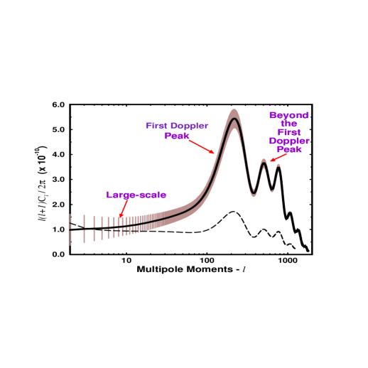
Figure 3.1: Angular power spectra predicted within inflationary cosmologies [from Steinhardt, 1995]. The spectra are for CDM and cosmological parameters $h=0.5~{},~{}\Omega_{B}=0.05$, with cosmological constant $\Lambda=0$.

Although we have not introduced so far the necessary notation and machinery for giving a ‘quantitative’ account of the many contributions to the CMB temperature anisotropies on the various angular scales, let us at least qualitatively depict what currently is though to be the ‘standard model’ for the fluctuations in the relic radiation.

In Figure 3.1 we show the generic prediction for the angular power spectrum from standard inflation plus CDM on all relevant angular scales, namely, from the very large ($\ell$ small) to the smallest scales (large $\ell$’s) currently probed by observations. In this figure, the upper solid curve comes from a primordial (power–law) spectrum of density fluctuations, with spectral index $n=1$ on large angular scales (those scales which suffered little or no evolution at all) and no gravitational wave contribution. Vertical hashmarks give an idea of the theoretical uncertainties inherent to the CMB anisotropies which go under the name ‘cosmic variance’ and, as we see from the plot, are specially relevant on large angular scales. The lower curve (dashed) is for $n=0.85$ and shows the apparent ‘tilt’ in the otherwise flat Sachs–Wolfe plateau; this fact leads to spectra with more power on large scale (as to be compared with the ‘flat’ Harrison–Zel’dovich spectrum $n=1$). This curve also shows how the corresponding spectrum gets modified when the amplitude on large scales is built up by both scalar and tensor modes (50–50 mixture at the quadrupole level in the plot). For scales well within the horizon at recombination (as is the case for $\ell\mathrel{\raise 1.29167pt\hbox{$>$\kern-7.5pt\lower 4.30554pt\hbox{$\sim$}}}150$) gravitational waves redshift away and thus the overall amplitude gets equally reduced (as to be compared with the case with solely scalar contribution to the anisotropies).

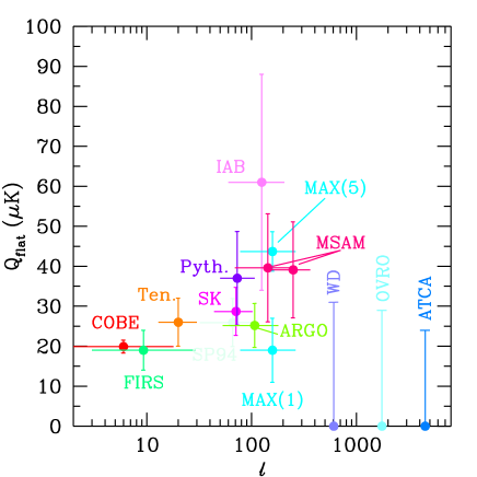
Figure 3.2: Amplitude of the fluctuations in different experiments, as a function of the scale (multipole $\ell\sim\theta^{-1}$) [from Scott et al., 1995]. ${\cal Q}_{flat}$ is the best–fitting amplitude of a flat power spectrum, given by $\ell(\ell+1){\cal C}_{\ell}=(24\pi/5)({\cal Q}_{flat}/T_{0})^{2}$.

While on large angular scales the observational results are well settled, on smaller scales the situation is not as clear. In Figure 3.2 we show the present status regarding observations. As it is clear from this figure there is some indication around scales $\ell\sim 200$ that the level of anisotropies grows, hinting for the existence of the Doppler peaks [Scott, Silk & White, 1995]. However, it is also apparent from the not always compatible data points and vertical error bars that presently nothing can be definitely concluded. More, independent pieces of observations are thus needed to corroborate the present experimental results and to fill in the gaps.

Chapter 4 CMB statistics

4.1 Dealing with spherical harmonics

In the following sections we will compute correlations of temperature anisotropies. The pattern of these anisotropies is distributed on the CMB sky two–sphere and, as such, it will prove useful to expand the temperature fluctuation field ${\Delta T\over T}$ (as we may do with any function that lives on a sphere) in spherical harmonics.

It is conventional to define the spherical harmonics in terms of the associated Legendre functions as follows

$$Y_{\ell}^{m}(\hat{\gamma})\equiv Y_{\ell}^{m}(\theta,\phi)=\sqrt{{2\ell+1\over 4\pi}{(\ell-m)!\over(\ell+m)!}}~{}P_{\ell}^{m}(\cos\theta)~{}e^{im\phi}$$ (4.1)

with $\ell$ and $m$ integers fulfilling the relations $\ell\geq 0$ and $|m|\leq\ell$.

As in the expression above we will often use the angles $\theta,\phi$ or the unit vector $\hat{\gamma}=(\sin\theta\cos\phi,\sin\theta\sin\phi,\cos\theta)$ interchangeably; when working with temperature anisotropies $\hat{\gamma}$ will be taken as the line–of–sight direction on the sky.

Being the product of $e^{im\phi}$, which form a complete set of orthogonal functions in the index $m$ on the interval $0\leq\phi\leq 2\pi$, and $P_{\ell}^{m}(\cos\theta)$, which form a similar set in the index $\ell$ for fixed $m$ on the interval $-1\leq\cos\theta\leq 1$, it is clear that the $Y_{\ell}^{m}$ will form an analogous set on the surface of the unit sphere in the two indices $\ell$, $m$.

Under complex conjugation they change as $Y_{\ell}^{-m}=(-1)^{m}{Y_{\ell}^{m}}^{*}$. The orthonormality condition is

$$\int d\Omega_{\hat{\gamma}}{Y_{\ell}^{m}}^{*}(\hat{\gamma})Y_{\ell^{\prime}}^{m^{\prime}}(\hat{\gamma})=\delta_{\ell\ell^{\prime}}\delta_{mm^{\prime}}$$ (4.2)

where the differential solid angle is given by $d\Omega_{\hat{\gamma}}=\sin\theta~{}d\theta~{}d\phi$. These properties, together with the completeness relation, allow one to expand any square–integrable function on the unit sphere, e.g., $\Delta$, as

$$\Delta(\hat{\gamma})=\sum_{\ell=0}^{\infty}\sum_{m=-\ell}^{\ell}a_{\ell}^{m}Y_{\ell}^{m}(\hat{\gamma})$$ (4.3)

where the complex quantities $a_{\ell}^{m}$ are given by

$$a_{\ell}^{m}=\int d\Omega_{\hat{\gamma}}{Y_{\ell}^{m}}^{*}(\hat{\gamma})\Delta(\hat{\gamma}).$$ (4.4)

We will be interested in the situation in which $\Delta$ is actually ${\Delta T\over T}$, the CMB temperature fluctuation, and in this case we will call $a_{\ell}^{m}$ the multipole moments. These are relevant quantities as in general predictions of a theory are expressed in terms of predictions for the $a_{\ell}^{m}$.

Also useful in this work is the spherical harmonics addition theorem

$$P_{\ell}(\cos\theta)={4\pi\over 2\ell+1}\sum_{m=-\ell}^{\ell}{Y_{\ell}^{m}}^{*}(\theta_{1},\phi_{1})Y_{\ell}^{m}(\theta_{2},\phi_{2})$$ (4.5)

This theorem applies to any spherical triangle on the unit sphere, with sides $\theta_{1}$, $\theta_{2}$ and $\theta$, and with the angle $|\phi_{1}-\phi_{2}|$ opposite to $\theta$, so that (being $\hat{\gamma}_{1}\equiv(\theta_{1},\phi_{1})$ and $\hat{\gamma}_{2}\equiv(\theta_{2},\phi_{2})$) we have $\hat{\gamma}_{1}\!\cdot\!\hat{\gamma}_{2}\equiv\cos\theta=\cos\theta_{1}\cos\theta_{2}+\sin\theta_{1}\sin\theta_{2}\cos|\phi_{1}-\phi_{2}|$.

The spherical harmonics as defined above are connected with the bases of the even (or single-valued) representations of the rotation group on the sphere.

We will see below that, when dealing with correlations, it will prove convenient to define the rotationally symmetric quantities $Q_{\ell}^{2}=\sum_{m=-\ell}^{\ell}|a_{\ell}^{m}|^{2}$, which we will call the multipole coefficients.

That the above defined quantities are rotationally symmetric can be seen from the fact that a suitable average over the $m$ index was performed. Given the expansion in spherical harmonics of any function

$$f(\hat{\gamma}_{1})=\sum_{\ell}\sum_{m}a_{\ell}^{m}Y_{\ell}^{m}(\hat{\gamma}_{1}),$$ (4.6)

one could wonder how the multipole moments change for a rotated version of the same function, say $f(\hat{\gamma}_{2})$, written in terms of the same $Y_{\ell}^{m}(\hat{\gamma}_{1})$’s. That is, we express $f(\hat{\gamma}_{2})=\sum_{\ell}\sum_{m}~{}^{(old)}\!a_{\ell}^{m}Y_{\ell}^{m}(\hat{\gamma}_{2})$ and, by recalling the relation

$$Y_{\ell}^{m}(\hat{\gamma}_{2})=\sum_{m^{\prime}}D^{\ell}_{m^{\prime}m}Y_{\ell}^{m^{\prime}}(\hat{\gamma}_{1})$$ (4.7)

we get $f(\hat{\gamma}_{2})=\sum_{\ell}\sum_{m^{\prime}}~{}^{(new)}a_{\ell}^{m^{\prime}}Y_{\ell}^{m^{\prime}}(\hat{\gamma}_{1})$ where we defined

$${}~{}^{(new)}a_{\ell}^{m^{\prime}}=\sum_{m}D^{\ell}_{m^{\prime}m}~{}^{(old)}a_{\ell}^{m}.$$ (4.8)

This means that after rotation the new $a_{\ell}^{m}$ are just a linear combination of the old ones, with $\ell$ index fixed. We see then that a rotation on the sphere will not change the multipole coefficients $Q_{\ell}^{2}$, which depend only on $\ell$.

Now going back to the defining expression for the $Q_{\ell}^{2}$, and baring in mind what we discussed above, we see that no matter how we rotate a given function the different $\ell$ contributions to it are independent and do not mix: say, if we focus on the dipole ($\ell=1$) contribution (the linear part), and we rotate, it will never pick up quadratic ($\ell=2$), cubic ($\ell=3$) or any other $\ell\neq 1$ terms.

4.2 The CMB two–point correlation function

Our main aim below will be to compute the CMB three–point temperature correlation function. The very existence of non–vanishing higher–order correlation functions on large angular scales is due to possible departures from a Gaussian behaviour of the primordial peculiar gravitational potential (cf. Chapter 5). Also, even for the case of primordial Gaussian curvature fluctuations, the mildly non–linear gravitational evolution gives rise to a non–vanishing three–point correlation function and we will see in Chapter 6 below what predictions we get for this integrated effect.

As a first step we will define the connected two– and three–point correlation functions of the CMB temperature anisotropies as measured by a given observer, i.e., on a single microwave sky. Let us then define the temperature fluctuation field ${\Delta T\over T}(\vec{x};\hat{\gamma})\equiv(T(\vec{x};\hat{\gamma})-T_{0}(\vec{x}))/T_{0}(\vec{x})$, where $\vec{x}$ specifies the position of the observer, the unit vector $\hat{\gamma}$ points in a given direction from $\vec{x}$ and $T_{0}(\vec{x})\equiv\int{d\Omega_{\hat{\gamma}}\over 4\pi}T(\vec{x};\hat{\gamma})$ represents the mean temperature of the CMB measured by that observer (i.e., the monopole term).

The angular two–point correlation function $C_{2}(\vec{x};\alpha)$ measured by an observer placed in $\vec{x}$ is the average product of temperature fluctuations in two directions $\hat{\gamma}_{1}$ and $\hat{\gamma}_{2}$ whose angular separation is $\alpha$; this can be written as

$$C_{2}(\vec{x};\alpha)=\int{d\Omega_{\hat{\gamma}_{1}}\over 4\pi}\int{d\Omega_{\hat{\gamma}_{2}}\over 2\pi}\delta\bigl{(}\hat{\gamma}_{1}\cdot\hat{\gamma}_{2}-\cos\alpha\bigr{)}{\Delta T\over T}(\vec{x};\hat{\gamma}_{1}){\Delta T\over T}(\vec{x};\hat{\gamma}_{2})\ .$$ (4.9)

As well known, in the limit $\alpha\to 0$ one recovers the CMB variance $C_{2}(\vec{x})=\int{d\Omega_{\hat{\gamma}}\over 4\pi}[{\Delta T\over T}(\vec{x};\hat{\gamma})]^{2}$. Expanding the temperature fluctuation in spherical harmonics

$${\Delta T\over T}(\vec{x};\hat{\gamma})=\sum_{\ell=1}^{\infty}\sum_{m=-\ell}^{\ell}a_{\ell}^{m}(\vec{x}){\cal W}_{\ell}Y_{\ell}^{m}(\hat{\gamma}),$$ (4.10)

and writing the Dirac delta function as a completeness relation for Legendre polynomials $P_{\ell}$

$$\delta\bigl{(}\cos\theta_{1}-\cos\theta_{2}\bigr{)}=\sum_{\ell=0}^{\infty}(\ell+{\textstyle{1\over 2}})P_{\ell}(\cos\theta_{1})P_{\ell}(\cos\theta_{2}),$$ (4.11)

we easily arrive at the expression

$$C_{2}(\vec{x};\alpha)={1\over 4\pi}\sum_{\ell}P_{\ell}(\cos\alpha)Q_{\ell}^{2}(\vec{x}){\cal W}^{2}_{\ell}\ ,$$ (4.12)

where $Q_{\ell}^{2}=\sum_{m=-\ell}^{\ell}|a_{\ell}^{m}|^{2}$.

It is standard to compare theory and experiments through the $a_{\ell}^{m}$. However real measurement of temperature anisotropies are limited by finite resolution and specific strategies are employed by the many current experimental settings. How to account in our definitions for this modeling of the real world? It has become conventional to include this piece of dirty physics by the use of a filter, limiting the range in $\ell$ (and hence, the angular scale) to which the experiment is sensitive, in the form of a window function. In the previous expressions ${\cal W}_{\ell}$ represents in fact the window function of the specific experiment. Setting ${\cal W}_{0}={\cal W}_{1}=0$ automatically accounts for both monopole and dipole subtraction.

Let us remind the reader that the subtraction techniques employed in current anisotropy experiments do not allow us to get a value for the monopole. Moreover, the dipole contribution present in the maps (essentially ${\Delta T\over T}\simeq{\textstyle{v\over c}}\cos\theta$, where $\theta$ is the angle between the direction of motion and that of observation – see §3.1) is considered to be mainly due to our peculiar motion with respect to the comoving rest frame of the CMB radiation.

We will often concentrate below on large angular scales. In the case of the COBE–DMR experiment the window function for $\ell\geq 2$ is ${\cal W}_{\ell}\simeq\exp\left[-{\textstyle{1\over 2}}\ell({\ell}+1)\sigma^{2}\right]$, where $\sigma$ is the dispersion of the antenna–beam profile, which measures the angular response of the detector [e.g., Wright et al., 1992]. In some cases the quadrupole term is also subtracted from the maps [e.g., Smoot et al., 1992]; in this case we also set ${\cal W}_{2}=0$.

4.3 The CMB three–point correlation function

The analogous expression for the angular three–point correlation function is obtained by taking the average product of temperature fluctuations in three directions $\hat{\gamma}_{1}$, $\hat{\gamma}_{2}$ and $\hat{\gamma}_{3}$ with fixed angular separations $\alpha$ (between $\hat{\gamma}_{1}$ and $\hat{\gamma}_{2}$), $\beta$ (between $\hat{\gamma}_{2}$ and $\hat{\gamma}_{3}$) and $\gamma$ (between $\hat{\gamma}_{1}$ and $\hat{\gamma}_{3}$); these angles have to satisfy the obvious inequalities $|\alpha-\gamma|\leq\beta\leq\alpha+\gamma$. One then has

$$C_{3}(\vec{x};\alpha,\beta,\gamma)=\int{d\Omega_{\hat{\gamma}_{1}}\over 4\pi}\int_{0}^{2\pi}{d\varphi_{12}\over 2\pi}\int_{-1}^{1}d\cos\vartheta_{12}\delta\bigl{(}\cos\vartheta_{12}-\cos\alpha\bigr{)}\int_{-1}^{1}d\cos\vartheta_{23}$$

$$\times\delta\bigl{(}\cos\vartheta_{23}-\cos\beta\bigr{)}\!\int_{-1}^{1}\!\!d\cos\vartheta_{13}\delta\bigl{(}\cos\vartheta_{13}-\cos\gamma\bigr{)}{\Delta T\over T}(\vec{x};\hat{\gamma}_{1}){\Delta T\over T}(\vec{x};\hat{\gamma}_{2}){\Delta T\over T}(\vec{x};\hat{\gamma}_{3}),$$

where $\cos\vartheta_{\alpha\beta}\equiv\hat{\gamma}_{\alpha}\cdot\hat{\gamma}_{\beta}$ and $\varphi_{12}$ is the azimuthal angle of $\hat{\gamma}_{2}$ on the plane orthogonal to $\hat{\gamma}_{1}$. The above relation can be rewritten in a form analogous to Eq.(4.9), namely

$$C_{3}(\vec{x};\alpha,\beta,\gamma)=N(\alpha,\beta,\gamma)\int{d\Omega_{\hat{\gamma}_{1}}\over 4\pi}\int{d\Omega_{\hat{\gamma}_{2}}\over 2\pi}\int{d\Omega_{\hat{\gamma}_{3}}\over 2}\delta\bigl{(}\hat{\gamma}_{1}\cdot\hat{\gamma}_{2}-\cos\alpha\bigr{)}$$ (4.14)

$$\times\delta\bigl{(}\hat{\gamma}_{2}\cdot\hat{\gamma}_{3}-\cos\beta\bigr{)}\delta\bigl{(}\hat{\gamma}_{1}\cdot\hat{\gamma}_{3}-\cos\gamma\bigr{)}{\Delta T\over T}(\vec{x};\hat{\gamma}_{1}){\Delta T\over T}(\vec{x};\hat{\gamma}_{2}){\Delta T\over T}(\vec{x};\hat{\gamma}_{3})\ ,$$

where $N(\alpha,\beta,\gamma)\equiv\sqrt{1-\!\cos^{2}\!\alpha-\!\cos^{2}\!\beta-\!\cos^{2}\!\gamma+\!2\cos\alpha\cos\beta\cos\gamma}$. Setting $\alpha=\beta=\gamma=0$ in these general expressions one obtains the CMB skewness $C_{3}(\vec{x})=\int{d\Omega_{\hat{\gamma}}\over 4\pi}[{\Delta T\over T}(\vec{x};\hat{\gamma})]^{3}$. Also useful are the equilateral three–point correlation function [e.g., Falk et al., 1993] and the collapsed one [e.g., Hinshaw et al., 1994 and references therein], corresponding to the choices $\alpha=\beta=\gamma$, and $\alpha=\gamma$, $\beta=0$, respectively. Alternative statistical estimators, more suited to discriminate bumpy non–Gaussian signatures in noisy data, have been recently introduced by Graham et al. [1993]. In all the above formulas, full–sky coverage was assumed, for simplicity. The effects of partial sky coverage on some of the statistical quantities considered here are discussed in detail by Scott, Srednicki & White [1994] (see also Ref.[37]).

Following the procedure used above for $C_{2}(\vec{x};\alpha)$, we can rewrite the three–point function in the form

$$C_{3}(\vec{x};\alpha,\beta,\gamma)=N(\alpha,\beta,\gamma){\pi\over 2}\sum_{\ell_{1},\ell_{2},\ell_{3}}\sum_{m_{1},m_{2},m_{3}}a_{\ell_{1}}^{m_{1}}a_{\ell_{2}}^{m_{2}}{a_{\ell_{3}}^{m_{3}}}^{*}{\cal W}_{\ell_{1}}{\cal W}_{\ell_{2}}{\cal W}_{\ell_{3}}$$ (4.15)

$$\times\sum_{j,k,\ell}\sum_{m_{j},m_{k},m_{\ell}}P_{j}(\cos\alpha)P_{k}(\cos\beta)P_{\ell}(\cos\gamma){\cal H}_{j\ell\ell_{1}}^{m_{j}m_{\ell}m_{1}}{\cal H}_{kj\ell_{2}}^{m_{k}m_{j}m_{2}}{\cal H}_{k\ell\ell_{3}}^{m_{k}m_{\ell}m_{3}}\ ,$$

where the coefficients ${\cal H}_{\ell_{1}\ell_{2}\ell_{3}}^{m_{1}m_{2}m_{3}}\equiv\int d\Omega_{\hat{\gamma}}{Y_{\ell_{1}}^{m_{1}}}^{*}(\hat{\gamma})Y_{\ell_{2}}^{m_{2}}(\hat{\gamma})Y_{\ell_{3}}^{m_{3}}(\hat{\gamma})$, which can be easily expressed in terms of Clebsch–Gordan coefficients [e.g., Messiah 1976], are only non–zero if the indices $\ell_{i}$, $m_{i}$ ($i=1,2,3,$) fulfill the relations: $|\ell_{j}-\ell_{k}|\leq\ell_{i}\leq|\ell_{j}+\ell_{k}|$, $\ell_{1}+\ell_{2}+\ell_{3}=even$ and $m_{1}=m_{2}+m_{3}$. We may occasionally in what follows make use of a related quantity $\bar{\cal H}_{\ell_{1}\ell_{2}\ell_{3}}^{m_{1}m_{2}m_{3}}\equiv(-1)^{m_{1}}{\cal H}_{~{}\ell_{1}\ell_{2}\ell_{3}}^{-m_{1}m_{2}m_{3}}$ which has the further advantage of being invariant under circular permutation of its columns $\left({}^{m_{i}}_{\ell_{i}}\right)$. In fact, this is apparent from the following expression in terms of the ‘3j’ symbols:

$$\bar{\cal H}_{\ell_{1}\ell_{2}\ell_{3}}^{m_{1}m_{2}m_{3}}=\left((2\ell_{1}+1)(2\ell_{2}+1)(2\ell_{3}+1)/4\pi\right)^{1/2}\left({}^{\ell_{1}~{}\ell_{2}~{}\ell_{3}}_{0~{}~{}0~{}~{}0}\right)\left({}^{\ell_{1}~{}\,\;\ell_{2}~{}\,\;\ell_{3}}_{m_{1}~{}m_{2}~{}m_{3}}\right)~{}.$$ (4.16)

The collapsed three–point function measured by the observer in $\vec{x}$ reads

$$C_{3}(\vec{x};\alpha)={1\over 4\pi}\sum_{\ell_{1},\ell_{2},\ell_{3}}\sum_{m_{1},m_{2},m_{3}}P_{\ell_{1}}(\cos\alpha)a_{\ell_{1}}^{m_{1}}a_{\ell_{2}}^{m_{2}}{a_{\ell_{3}}^{m_{3}}}^{*}{\cal W}_{\ell_{1}}{\cal W}_{\ell_{2}}{\cal W}_{\ell_{3}}{\cal H}_{\ell_{3}\ell_{2}\ell_{1}}^{m_{3}m_{2}m_{1}}$$ (4.17)

which, for $\alpha=0$, gives a useful expression for the skewness.

4.4 Predictions of a theory: ensemble averages

To obtain definite predictions for the statistics described above, one needs to exploit the random nature of the multipole moments $a_{\ell}^{m}$. These coefficients tell us about the underlying theory for the generation of temperature fluctuations and, depending on the case, will be taken as following a Gaussian statistics (in which case predictions are fully specified by giving the two–point function for the $a_{\ell}^{m}$’s) or, more generally, a non–Gaussian one (and in this case also the bispectrum will be needed, as we will show below). In either case, the $a_{\ell}^{m}$’s are stochastic random variables of position, with zero mean and rotationally invariant variance depending only on $\ell$: $\bigl{\langle}a_{\ell}^{m}(\vec{x})\bigr{\rangle}=0$ and

$$\bigl{\langle}a_{\ell_{1}}^{m_{1}}(\vec{x}){a_{\ell_{2}}^{m_{2}}}^{*}(\vec{x})\bigr{\rangle}=\delta_{\ell_{1}\ell_{2}}\delta_{m_{1}m_{2}}{\cal C}_{\ell_{1}}\ ,$$ (4.18)

where brackets $\bigl{\langle}\cdot\bigr{\rangle}$ stand for an average over the ensemble of possible universes.

Within standard inflationary models, fluctuations are Gaussian and therefore knowing the ${\cal C}_{\ell}$’s is enough for characterising the angular fluctuation spectrum. The ${\cal C}_{\ell}$’s however are not trivial to compute, specially on small scales (large $\ell$) where they encode crucial information regarding the cosmological parameters. On the other hand, on large scales where the Sachs–Wolfe contribution to the anisotropy is likely to dominate the signal, we have ${\Delta T\over T}(\vec{x};\hat{\gamma})={1\over 3}\Phi(\vec{x}+r_{0}\hat{\gamma})$, with $r_{0}=2/H_{0}$ the horizon distance and $H_{0}$ the Hubble constant, and the multipole coefficients are given by

$${\cal C}_{\ell}\propto\int_{0}^{\infty}dkk^{2}P_{\Phi}(k)j_{\ell}^{2}(kr_{0})\ ,$$ (4.19)

where $P_{\Phi}(k)$ is the gravitational potential power–spectrum and $j_{\ell}$ is the $\ell$–th order spherical Bessel function.

For large scales we can make the approximation $P_{\Phi}(k)\propto k^{n-4}$, where $n$ corresponds to the primordial index of density fluctuations (e.g., $n=1$ is the Zel’dovich, scale invariant case), in which case [e.g., Bond & Efstathiou, 1987; Fabbri, Lucchin & Matarrese, 1987]

$${\cal C}_{\ell}={{\cal Q}^{2}\over 5}{\Gamma(\ell+n/2-1/2)\Gamma(9/2-n/2)\over\Gamma(\ell+5/2-n/2)\Gamma(3/2+n/2)},$$ (4.20)

with ${\cal Q}=\bigl{\langle}Q_{2}^{2}\bigr{\rangle}^{1/2}$ the rms quadrupole, which is simply related to the quantity $Q_{rms-PS}$ defined by [Smoot et al., 1992]: ${\cal Q}=\sqrt{4\pi}Q_{rms-PS}/T_{0}$.

Notice that for the quadrupole we get ${\cal C}_{\ell=2}={\cal Q}^{2}/5$, and this depends on the spectral index $n$ (i.e., the normalisation of the fluctuation spectrum depends on the form of the spectrum). If we instead take $n=1$ we get $\ell(\ell+1){\cal C}_{\ell}=6{\cal Q}^{2}/5$, which is independent of the multipole index $\ell$. This is often referred to as a ‘flat’ spectrum, since gravitational potential fluctuations (as well as the amplitude of the density contrast at horizon crossing) are independent of the scale.

Roughly speaking the amplitude for ${\cal C}_{\ell}$ is determined by fluctuations on angular scales $\theta\sim\pi/\ell$ radians. As we mentioned in Chapter 3, a plot of $\ell(\ell+1){\cal C}_{\ell}$ is usually referred to as the angular power spectrum. With this definition an exact $n=1$ initial spectrum, assuming the relevant scales suffered virtually no evolution after becoming smaller than the horizon (as is the case for very large scales), produces a flat spectrum (a ‘plateau’ in the $\ell(\ell+1){\cal C}_{\ell}$ vs. $\ell$ plot).

Inflationary theories predict tensor metric fluctuations, in addition to (and statistically independent of) scalar modes. As a consequence, the total multipole moment is actually the sum of two orthogonal contributions, which are ordinarily noted as ${\cal C}^{(T)}_{\ell}$ and ${\cal C}^{(S)}_{\ell}$ for tensor and scalar, respectively. Tilted ($n<1$) models, as are predicted by e.g., power–law inflation, some versions of intermediate inflation, natural inflation and a few other models, imply more power (relative to a flat spectrum) on large scales and consequently enhance the contribution from long wavelength tensor modes (gravitational waves). This is of relevance for the correct normalisation of the spectrum on large scales, as it is the actual case after the detection of anisotropies in the COBE–DMR maps.

Chapter 5 Primordial non–Gaussian features

It has been realised that inflationary models also predict small deviations from Gaussianity. Every sensible inflation model will produce some small but non–negligible non–Gaussian effects, both by the self–interaction of the inflaton field, and by the local back–reaction of its self–gravity. It is our interest here to quantify this prediction, with the largest possible generality, so that observational results on the CMB angular three–point function can be used as a further test on the nature of the primordial perturbation process.

Unfortunately, we will find that single–field inflation models generally imply mean values for the skewness which are well below the cosmic rms skewness of a Gaussian field, which confirms and generalises earlier results based on a simple toy–model [Falk, Rangarajan & Srednicki, 1993; Srednicki, 1993].

Falk et al.  [1993] first gave a quantitative estimate of the size of non–Gaussian effects through a calculation of the three–point CMB correlation function from perturbations generated in a simple model, where the inflaton has cubic self–interactions.

Here the problem is considered in a totally general and self–consistent way. We use the stochastic approach to inflation [e.g., Starobinskii, 1986; Goncharov, Linde & Mukhanov, 1987; see also §2.1.7], as a technical tool to self–consistently account for all second–order effects in the generation of scalar field fluctuations during inflation and their giving rise to curvature perturbations. We also properly account for the non–linear relation between the inflaton fluctuation and the peculiar gravitational potential. Our derivation moreover removes a non–realistic restriction to purely de Sitter background made by Falk et al.  [1993], which is especially important when non–Zel’dovich perturbation spectra are considered.

The technical derivation in the frame of stochastic inflation of the connected two– and three–point function (or its Fourier counterpart, the bispectrum), for the inflaton field first and the local gravitational potential next, is reported in §5.1. From this we compute (§5.2) the CMB temperature anisotropy bispectrum and apply it to the collapsed three–point function. §5.3 deals with the zero–lag limit of the three–point function: the skewness, for which we provide a universal inflationary expression, which we then specialise to some of the most popular inflaton potentials: exponential [Lucchin & Matarrese, 1985], quartic and quadratic [Linde, 1983, 1985] as well as a simple potential for hybrid inflation [Linde, 1994]. Interestingly enough, this last model allows for a spectral index greater than one. In §5.4 we discuss the effects of the cosmic variance on the possibility of observing a non–zero mean value for the skewness. As a by–product of this analysis we compute the ‘dimensionless’ rms skewness for a large range of the primordial spectral index of density fluctuations $n$. Finally, we provide a brief discussion in §5.5

5.1 Stochastic inflation and the statistics of the gravitational potential

In order to take into account all the effects contributing to a non–vanishing primordial three–point correlation function of $\Phi$, we will perform the computation in two steps. In §5.1.1 we compute the three–point function for the inflaton field perturbation $\delta\phi$. The most convenient way to perform this calculation is in the frame of the stochastic approach to inflation [Starobinskii, 1986; Goncharov et al., 1987], which naturally takes into account all the multiplicative effects in the inflaton dynamics that are responsible for the non–Gaussian features. Then, in §5.1.2 we compute the extra–contribution to the three–point function of the gravitational potential that arises due to the non–linear relation between $\Phi$ and $\delta\phi$. This effect has been previously noticed by Barrow & Coles [1990] and Yi & Vishniac [1993].

5.1.1 The inflaton bispectrum

To study the dynamics of the inflaton, we will apply the stochastic approach. This is based on defining a coarse–grained inflaton field $\phi(\vec{x},\alpha)$, obtained by suitable smoothing of the original quantum field over a scale larger than the Hubble radius size, whose dynamics is described by a multiplicative Langevin–type equation (cf. §2.1.7). This is obtained by adding to the classical equation of motion a Gaussian noise term whose amplitude is fixed by the rms fluctuation of the scalar field at Hubble radius crossing,

$${\partial\phi(\vec{x},\alpha)\over\partial\alpha}=-{m_{P}^{2}V^{\prime}(\phi)\over 8\pi V(\phi)}+{H(\phi)\over 2\pi}\eta(\vec{x},\alpha)\ ,$$ (5.1)

where $V(\phi)$ is the inflaton potential, primes denote differentiation with respect to $\phi$ and $m_{P}$ is the Planck mass. The Hubble parameter here should be consistently calculated from the local energy density of the coarse–grained inflaton. The noise term $\eta$ has zero mean and autocorrelation function [e.g., Mollerach et al., 1991]

$$\bigl{\langle}\eta(\vec{x},\alpha)\eta(\vec{x}^{\prime},\alpha^{\prime})\bigr{\rangle}=j_{0}(q_{s}(\alpha)|\vec{x}-\vec{x}^{\prime}|)\delta(\alpha-\alpha^{\prime})\ .$$ (5.2)

The use of the time variable $\alpha=\ln\left(a/a_{*}\right)$ in this equation has been motivated by Starobinskii [1986], who noticed that $\alpha$ accounts for the possible time dependence of the Hubble parameter. This is particularly relevant when general, i.e. non–de Sitter, inflation is studied. We also defined the coarse–grained domain size through the comoving wave–number $q_{s}(\alpha)\equiv\epsilon H(\alpha)a(\alpha)$, with $\epsilon$ a number smaller than one, $H(\alpha)\equiv H(\phi_{cl}(\alpha))$, with $\phi_{cl}(\alpha)$ the homogeneous classical solution of the Langevin equation (i.e., that obtained with the noise term ‘switched’ off). Finally the scale factor $a(\alpha)$ is obtained by integration of $H(\alpha)$.

The stochastic dynamics of the coarse–grained field within a single coarse–graining domain (i.e., for $\vec{x}=\vec{x}^{\prime}$) can be studied in terms of the Fokker–Planck equation for the probability distribution function of $\phi$. In our case, instead, since we are interested also in spatial correlations of the field, we will solve directly the Langevin equation above. To the aim of computing the three–point function of $\phi$, a second–order perturbative expansion around the classical solution is enough. We will require that the potential $V(\phi)$ is a smooth function of its argument, which translates into requiring well defined values for the steepness of the potential $X(\alpha)\equiv X(\phi_{cl}(\alpha))\equiv m_{P}V^{\prime}(\phi_{cl})/V(\phi_{cl})$ and its derivatives [Turner, 1993] throughout the range of relevant scales. Apart from this requirement we keep the analysis general; only at the end we will apply our results to some specific inflationary potentials (§§5.3.1–5.3.2). We first expand $V(\phi)$ around $\phi_{cl}$, up to second order in $\delta\phi(\vec{x},\alpha)\equiv\phi(\vec{x},\alpha)-\phi_{cl}(\alpha)$, $V(\phi)=V(\phi_{cl})+V^{\prime}(\phi_{cl})\delta\phi+{\textstyle{1\over 2}}V^{\prime\prime}(\phi_{cl})\delta\phi^{2}+\cdots$. Replacing this into the Langevin equation we obtain

$${\partial\delta\phi(\vec{x},\alpha)\over\partial\alpha}=A(\alpha)\delta\phi(\vec{x},\alpha)+B(\alpha)\delta\phi^{2}(\vec{x},\alpha)+\left[D_{1}(\alpha)+D_{2}(\alpha)\delta\phi(\vec{x},\alpha)\right]\eta(\vec{x},\alpha)\ ,$$ (5.3)

where we have used $\partial\phi_{cl}/\partial\alpha=-m_{P}^{2}V^{\prime}(\phi_{cl})/(8\pi V(\phi_{cl}))$. In Eq.(5.3) we defined

$$A=-{m_{P}\over 8\pi}X^{\prime}{}~{};~{}B=-{m_{P}\over 16\pi}X^{\prime\prime}{}~{};~{}D_{1}={H(\alpha)\over 2\pi}{}~{};~{}D_{2}={H(\alpha)X\over 4\pi m_{P}}\ .$$ (5.4)

Let us now split the field perturbation as $\delta\phi=\delta\phi_{1}+\delta\phi_{2}$ of first and second order, respectively. We can also define a rescaled variable $\tilde{\eta}\equiv(H(\alpha)/2\pi)\eta$. We then find

$$\delta\phi_{1}(\vec{x},\alpha)=X(\alpha)\int_{0}^{\alpha}d\alpha^{\prime}X^{-1}(\alpha^{\prime})\tilde{\eta}(\vec{x},\alpha^{\prime})$$ (5.5)

$$\delta\phi_{2}(\vec{x},\alpha)=X(\alpha)\int_{0}^{\alpha}d\alpha^{\prime}\left[{B(\alpha^{\prime})\over X(\alpha^{\prime})}\delta\phi_{1}^{2}(\vec{x},\alpha^{\prime})+{1\over 2m_{P}}\delta\phi_{1}(\vec{x},\alpha^{\prime})\tilde{\eta}(\vec{x},\alpha^{\prime})\right]\ .$$ (5.6)

Let us now calculate the connected three–point correlation function of $\delta\phi$. The lowest order non–vanishing contribution reads

$$\bigl{\langle}\delta\phi(\vec{x}_{1},\alpha_{1})\delta\phi(\vec{x}_{2},\alpha_{2})\delta\phi(\vec{x}_{3},\alpha_{3})\bigr{\rangle}=$$ (5.7)

$$\!X(\alpha_{3})\!\int_{0}^{\alpha_{3}}\!d\alpha^{\prime}\left[{B(\alpha^{\prime})\over X(\alpha^{\prime})}\bigl{\langle}\delta\phi_{1}(\vec{x}_{1},\alpha_{1})\delta\phi_{1}(\vec{x}_{3},\alpha^{\prime})\bigr{\rangle}\bigl{\langle}\delta\phi_{1}(\vec{x}_{2},\alpha_{2})\delta\phi_{1}(\vec{x}_{3},\alpha^{\prime})\bigr{\rangle}\!+\![\vec{x}_{1}\!\leftrightarrow\!\vec{x}_{2}]\right]$$

$$+{X(\alpha_{3})\over 2m_{P}}\!\int_{0}^{\alpha_{3}}\!d\alpha^{\prime}\left[\bigl{\langle}\delta\phi_{1}(\vec{x}_{1},\alpha_{1})\delta\phi_{1}(\vec{x}_{3},\alpha^{\prime})\bigr{\rangle}\bigl{\langle}\delta\phi_{1}(\vec{x}_{2},\alpha_{2})\tilde{\eta}(\vec{x}_{3},\alpha^{\prime})\bigr{\rangle}\!+\![\vec{x}_{1}\!\leftrightarrow\!\vec{x}_{2}]\right]$$

$$+~{}2\times 2~{}terms\ .$$

The term proportional to $X(\alpha_{3})/2m_{P}$ in the r.h.s. of this equation can be recast in the form

$${X(\alpha_{2})X(\alpha_{3})\over 2m_{P}}\!\int_{0}^{\alpha_{min}}\!\!d\alpha^{\prime}X^{-1}(\alpha^{\prime})\!{H^{2}(\alpha^{\prime})\over(2\pi)^{2}}\!\bigl{\langle}\delta\phi_{1}(\vec{x}_{1},\alpha_{1})\delta\phi_{1}(\vec{x}_{3},\alpha^{\prime})\bigr{\rangle}{}~{}j_{0}(q_{s}(\alpha^{\prime})|\vec{x}_{2}-\vec{x}_{3}|)$$ (5.8)

where we defined $\alpha_{min}\equiv{\rm min}[\alpha_{3},\alpha_{2}]$. We need now to compute the $\delta\phi$ autocorrelation function. To this aim, recalling that $\alpha$ is the time when the perturbation wavelength $\sim a/q$ equals the size of the coarse–graining domain, we change the integration variable in Eq. (5.5)) from $\alpha$ to $q=\sqrt{8\pi V(\alpha)/3}~{}q_{*}e^{\alpha}/H_{*}m_{P}$. The subscript $*$ denotes quantities evaluated at the time when we start to solve the Langevin equation; this is chosen in such a way that the patch of the universe where we live is homogeneous on a scale slightly above our present horizon [see, e.g., the discussion by Mollerach et al., 1991]. We then find

$$\bigl{\langle}\delta\phi_{1}(\vec{x}_{1},\alpha_{1})\delta\phi_{1}(\vec{x}_{3},\alpha^{\prime})\bigr{\rangle}={1\over 2\pi^{2}}\int_{q_{*}}^{q_{min}(q_{1},q^{\prime})}dqq^{2}P(q){X(q_{1})X(q^{\prime})\over X(q)X(q)}j_{0}(q|\vec{x}_{1}-\vec{x}_{3}|)$$ (5.9)

where we defined $P(q)\equiv{1\over 2}q^{-3}H^{2}(q)$ where $\alpha=\alpha(q)$. Using this we can rewrite Eq. (5.8) as

$${X(q_{1})X(q_{2})X(q_{3})\over 2m_{P}}\int{d^{3}q^{\prime}\over(2\pi)^{3}}\int{d^{3}q\over(2\pi)^{3}}{P(q^{\prime})P(q)\over X^{2}(q)}$$ (5.10)

$$\times W(q^{\prime};q_{min}(q_{3},q_{2}))W(q;q_{min}(q_{1},q^{\prime}))e^{i\vec{q}\cdot(\vec{x}_{1}-\vec{x}_{3})}e^{i{\vec{q}}^{\prime}\cdot(\vec{x}_{2}-\vec{x}_{3})}$$

where we defined the filter function $W(q;q_{i})\equiv\Theta(q-q_{*})-\Theta(q-q_{i})$ ($\Theta$ is the Heaviside function).

A similar analysis can be performed for the term proportional to $B(\alpha)$ in Eq. (5.7). We get

$$X(q_{1})X(q_{2})X(q_{3})\int_{q_{*}}^{q_{3}}{dq^{\prime}\over q^{\prime}}B(q^{\prime})X(q^{\prime})\int{d^{3}q^{\prime\prime}\over(2\pi)^{3}}\int{d^{3}q^{\prime\prime\prime}\over(2\pi)^{3}}{P(q^{\prime\prime})\over X^{2}(q^{\prime\prime})}{P(q^{\prime\prime\prime})\over X^{2}(q^{\prime\prime\prime})}$$ (5.11)

$$\times W(q^{\prime\prime\prime};q_{min}(q_{2},q^{\prime}))W(q^{\prime\prime};q_{min}(q_{1},q^{\prime}))e^{i{\vec{q}}^{\prime\prime}\cdot(\vec{x}_{1}-\vec{x}_{3})}e^{i{\vec{q}}^{\prime\prime\prime}\cdot(\vec{x}_{2}-\vec{x}_{3})}\ .$$

So far we have been working in configuration space. In order to obtain the gravitational potential at Hubble radius crossing during the Friedmann era, it is convenient to Fourier transform the coarse–grained inflaton fluctuation. One has $\delta\phi(\vec{x},\alpha(q))=(2\pi)^{-3}\int d^{3}k~{}\delta\phi(\vec{k})\Theta(q-k)e^{i\vec{k}\cdot\vec{x}}$, where $\delta\phi(\vec{k})$ denotes the Fourier transform of the full scalar field at the time $\alpha(q)$. This follows from the fact that at the time $\alpha(q)$ the only modes $k$ that contribute to the coarse–grained variable are those which have already left the inflationary horizon, namely $k<q$. We can then obtain the Fourier transform $\delta\phi(\vec{k},\alpha(q))=\delta\phi(\vec{k})\Theta(q-k)$, and, in the limit $k\to q^{-}$ (or equivalently $q\to k^{+}$, that is, when we consider the horizon–crossing time of the given scale), we simply have $\delta\phi(\vec{k},\alpha(k))=\delta\phi(\vec{k})$. In other words, at the time $\alpha(k)$ the Fourier transform of the coarse–grained variable coincides with that of the full field. Using these results in Eq. (5.7) we finally obtain the inflaton bispectrum through

$$\bigl{\langle}\delta\phi(\vec{k}_{1},\alpha(k_{1}))\delta\phi(\vec{k}_{2},\alpha(k_{2}))\delta\phi(\vec{k}_{3},\alpha(k_{3}))\bigr{\rangle}=(2\pi)^{3}\delta^{3}(\vec{k}_{1}+\vec{k}_{2}+\vec{k}_{3})P(k_{2})P(k_{3})$$ (5.12)

$$\times{X(k_{1})\over X(k_{2})X(k_{3})}\left[{X^{2}(k_{2})\Theta(k_{2}-k_{3})+X^{2}(k_{3})\Theta(k_{3}-k_{2})\over 2m_{P}}+2\int_{k_{*}}^{k_{1}}{dq^{\prime}\over q^{\prime}}B(q^{\prime})X(q^{\prime})\right]$$

$$+\{\vec{k}_{1}\!\leftrightarrow\!\vec{k}_{2}\}+\{\vec{k}_{1}\!\leftrightarrow\!\vec{k}_{3}\}\ .$$

5.1.2 The three–point function of the gravitational potential

We want now to compute the three–point function of the peculiar gravitational potential, $\bigl{\langle}\Phi(r_{0}\hat{\gamma}_{1})\Phi(r_{0}\hat{\gamma}_{2})\Phi(r_{0}\hat{\gamma}_{3})\bigr{\rangle}$. The approximate constancy of the gauge–invariant quantity $\zeta$ outside the horizon [e.g., Bardeen, Steinhardt & Turner, 1983] allows to obtain the gravitational potential during the matter–dominated era, given the value of $\delta\phi$ during inflation. During inflation one has $\zeta(\vec{x},\alpha)\simeq-\delta\phi(\vec{x},\alpha)/(\partial\phi/\partial\alpha)$, which is usually interpreted as a linear relation between $\zeta$ and $\delta\phi$. However, when calculating the three–point function of $\Phi$ one cannot disregard the second–order effects coming from the fluctuations of $\partial\phi/\partial\alpha$.

Recalling that

$${\partial\phi\over\partial\alpha}=-{m_{P}^{2}\over 8\pi}{V^{\prime}(\phi)\over V(\phi)}\simeq-{m_{P}\over 8\pi}\left[X(\alpha)+X^{\prime}(\alpha)\delta\phi\right]$$ (5.13)

one gets

$$\zeta(\vec{x})={8\pi\over m_{P}X(\alpha)}\left(\delta\phi(\vec{x},\alpha)-{X^{\prime}(\alpha)\over X(\alpha)}\delta\phi^{2}(\vec{x},\alpha)\right)\ .$$ (5.14)

This equation is expressed in configuration space; the Fourier transform of the first term inside the brackets is just $\delta\phi(\vec{k},\alpha)$. For the second term we get a convolution of the type $\int d^{3}p\delta\phi(\vec{p})\delta\phi(\vec{k}-\vec{p})$. For the scales of interest one has $\Phi(\vec{k})\simeq-3\zeta(\vec{k})/5$. Then, adding the two above contributions and evaluating the expression at the horizon crossing time we get

$$\Phi(\vec{k})\!=\!{24\pi\over 5m_{P}X(\alpha(k))}\!\!\left[\!\delta\phi(\vec{k},\alpha(k)\!)\!-{X^{\prime}(\!\alpha(k)\!)\over X(\!\alpha(k)\!)}\!\!\int\!\!\!{d^{3}p\over(2\pi)^{3}}\delta\phi(\vec{p},\alpha(k))\delta\phi(\vec{k}\!-\!\vec{p},\alpha(k))\!\right].$$ (5.15)

From this equation we calculate

$$\bigl{\langle}\Phi(\vec{k}_{1})\Phi(\vec{k}_{2})\Phi(\vec{k}_{3})\bigr{\rangle}={\left(24\pi/5m_{P}\right)^{3}\over X(k_{1})X(k_{2})X(k_{3})}\bigl{\langle}\delta\phi(\vec{k}_{1})\delta\phi(\vec{k}_{2})\delta\phi(\vec{k}_{3})\bigr{\rangle}+$$ (5.16)

$$\!+{\left(-24\pi/5m_{P}\right)^{3}X^{\prime}(k_{1})\over X^{2}(k_{1})X(k_{2})X(k_{3})}\int{d^{3}p\over(2\pi)^{3}}\bigl{\langle}\delta\phi(\vec{p})\delta\phi(\vec{k}_{1}-\vec{p})\delta\phi(\vec{k}_{2})\delta\phi(\vec{k}_{3})\bigr{\rangle}$$

$$\!+\{\vec{k}_{1}\!\leftrightarrow\!\vec{k}_{2}\}+\{\vec{k}_{1}\!\leftrightarrow\!\vec{k}_{3}\}$$

Using the fact that, at horizon crossing, $\bigl{\langle}\delta\phi(\vec{k}_{1})\delta\phi(\vec{k}_{2})\bigr{\rangle}=(2\pi)^{3}P(k_{1})\delta^{3}(\vec{k}_{1}+\vec{k}_{2})$, we can write

$$\bigl{\langle}\Phi(\vec{k}_{1})\Phi(\vec{k}_{2})\bigr{\rangle}=(2\pi)^{3}\delta^{3}(\vec{k}_{1}+\vec{k}_{2})f^{2}(\alpha(k_{1}))P(k_{1})\ ,$$ (5.17)

with $f(\alpha(k))\equiv 24\pi/5m_{P}X(\alpha(k))$. Finally, using Eqs. (5.17) and (5.12) we find

$$\bigl{\langle}\Phi(\vec{k}_{1})\Phi(\vec{k}_{2})\Phi(\vec{k}_{3})\bigr{\rangle}=\left({24\pi\over 5m_{P}}\right)^{3}(2\pi)^{3}\delta^{3}(\vec{k}_{1}+\vec{k}_{2}+\vec{k}_{3}){P(k_{2})\over X^{2}(k_{2})}{P(k_{3})\over X^{2}(k_{3})}$$ (5.18)

$$\!\times\left\{{X^{2}(k_{2})\Theta(k_{2}-k_{3})+X^{2}(k_{3})\Theta(k_{3}-k_{2})\over 2m_{P}}-{2X^{\prime}(k_{1})X(k_{2})X(k_{3})\over X^{2}(k_{1})}+\right.$$

$$\left.+2\int_{k_{*}}^{k_{1}}{dq^{\prime}\over q^{\prime}}B(q^{\prime})X(q^{\prime})\right\}+\{\vec{k}_{1}\!\leftrightarrow\!\vec{k}_{2}\}+\{\vec{k}_{1}\!\leftrightarrow\!\vec{k}_{3}\}$$

We are interested in considering perturbation modes that left the horizon about 60 e–foldings before the end of the inflationary epoch. In the explicit examples below $X(k)$ turns out to be a slowly varying function of $k$. We therefore approximate the steepness $X(k)\sim X_{60}$ in what follows. Then, to the lowest non–vanishing order, the three–point correlation function is

$$\bigl{\langle}\Phi(\vec{k}_{1})\Phi(\vec{k}_{2})\Phi(\vec{k}_{3})\bigr{\rangle}={1\over f_{60}}\left[{X_{60}\over 2m_{P}}-{2X^{\prime}_{60}\over X_{60}}+{2\over X_{60}}\int_{k_{*}}^{k_{60}}{dq\over q}B(\alpha(q))X(\alpha(q))\right]$$ (5.19)

$$\times~{}(2\pi)^{3}\delta^{3}(\vec{k}_{1}+\vec{k}_{2}+\vec{k}_{3})\left[P_{\Phi}(k_{1})P_{\Phi}(k_{2})+P_{\Phi}(k_{2})P_{\Phi}(k_{3})+P_{\Phi}(k_{3})P_{\Phi}(k_{1})\right]$$

with $f_{60}\equiv 24\pi/5m_{P}X_{60}$. Using the expression for $P(q)$ we obtain the power–spectrum for the peculiar gravitational potential

$$P_{\Phi}(k)=2\pi^{2}f_{60}^{2}k^{-3}H^{2}(\alpha(k))/4\pi^{2}\simeq{1\over 2}f_{60}^{2}H_{60}^{2}k^{-3}(k/k_{*})^{n-1},$$ (5.20)

up to possible presence of small logarithmic corrections. In this equation we used the fact that the variance per $\ln k$ of the perturbation in the $\zeta$ variable, ${\cal P}_{\zeta}=k^{3}P_{\zeta}/(2\pi^{2})\propto k^{n-1}$ is given at horizon crossing by $\sim(2\pi)^{-2}H^{4}/\dot{\phi}^{2}$. By using the equation of motion for the inflaton field, $2\dot{H}\simeq-8\pi\dot{\phi}^{2}/m_{P}^{2}$ we then have $H^{4}/\dot{\phi}^{2}\propto H^{4}/\dot{H}\propto t^{-2}\propto H^{2}$ (with $a\propto t^{p}$ and $p>1$ during inflation), and so $H^{2}\propto k^{n-1}$, as was in fact used in the second equality in Eq. (5.20) above.

5.2 The CMB angular bispectrum

Now we can obtain the two– and three–point correlation functions for $\Phi$ in configuration space by inverse Fourier transforming Eqs. (5.17) and (5.19). We then get the following general expressions for the mean two– and three–point functions of the primordial gravitational potential

$$\bigl{\langle}\Phi(r_{0}\hat{\gamma}_{1})\Phi(r_{0}\hat{\gamma}_{2})\bigr{\rangle}={9\over 4\pi}\sum_{\ell\geq 0}(2\ell+1)P_{\ell}(\hat{\gamma}_{1}\cdot\hat{\gamma}_{2}){\cal C}_{\ell}$$ (5.21)

and

$$\bigl{\langle}\Phi(r_{0}\hat{\gamma}_{1})\Phi(r_{0}\hat{\gamma}_{2})\Phi(r_{0}\hat{\gamma}_{3})\bigr{\rangle}={81\over(4\pi)^{2}}\Phi_{3}\sum_{j,\ell\geq 0}(2j+1)(2\ell+1){\cal C}_{j}{\cal C}_{\ell}$$ (5.22)

$$\times\bigl{[}P_{j}(\hat{\gamma}_{1}\cdot\hat{\gamma}_{3})P_{\ell}(\hat{\gamma}_{1}\cdot\hat{\gamma}_{2})+P_{j}(\hat{\gamma}_{2}\cdot\hat{\gamma}_{1})P_{\ell}(\hat{\gamma}_{2}\cdot\hat{\gamma}_{3})+P_{j}(\hat{\gamma}_{3}\cdot\hat{\gamma}_{1})P_{\ell}(\hat{\gamma}_{3}\cdot\hat{\gamma}_{2})\bigr{]}\ ,$$

where now the rms quadrupole (cf. Eq. (4.20)) for the multipole coefficients is given by

$${\cal Q}^{2}={8\pi^{2}H_{60}^{2}\over 5m_{P}^{2}X_{60}^{2}}{\Gamma(3-n)\Gamma(3/2+n/2)\over\Gamma^{2}(2-n/2)\Gamma(9/2-n/2)}$$ (5.23)

and

$$\Phi_{3}={1\over f_{60}}\left[{X_{60}\over 2m_{P}}-{2X^{\prime}_{60}\over X_{60}}+{2\over X_{60}}\int_{k_{*}}^{k_{60}}{dq\over q}B(\alpha(q))X(\alpha(q))\right]$$ (5.24)

In order to obtain Eqs. (5.21) and (5.22), we had to use the definition of ${\cal C}_{\ell}$. The one given in §4.4 differs from the results obtained here because of the window function $W(k)$, appearing in the inflationary expressions; this can be however neglected if we account for the oscillating behaviour of $j_{\ell}$ for large arguments and for the fact that $j_{\ell}\to 0$ for small arguments (that helps in cancelling the lower divergence).

The equations above allow us to recover Eq. (4.18) for the angular spectrum, and the following expression for the angular bispectrum,

$$\bigl{\langle}a_{\ell_{1}}^{m_{1}}a_{\ell_{2}}^{m_{2}}{a_{\ell_{3}}^{m_{3}}}^{*}\bigr{\rangle}=3\Phi_{3}\bigl{[}{\cal C}_{\ell_{1}}{\cal C}_{\ell_{2}}+{\cal C}_{\ell_{2}}{\cal C}_{\ell_{3}}+{\cal C}_{\ell_{3}}{\cal C}_{\ell_{1}}\bigr{]}{\cal H}_{\ell_{3}\ell_{1}\ell_{2}}^{m_{3}m_{1}m_{2}}\ .$$ (5.25)

Replacing the latter expression into Eq. (4.15) we obtain the general form of the mean three–point correlation function. Some simplifications occur for the collapsed three–point function, for which we obtain

$$\bigl{\langle}C_{3}(\alpha)\bigr{\rangle}={3\over(4\pi)^{2}}\Phi_{3}\sum_{\ell_{1},\ell_{2},\ell_{3}}P_{\ell_{1}}(\cos\alpha){\cal F}_{\ell_{1}\ell_{2}\ell_{3}}$$ (5.26)

$$\times(2\ell_{1}+1)(2\ell_{2}+1)(2\ell_{3}+1)\bigl{[}{\cal C}_{\ell_{1}}{\cal C}_{\ell_{2}}+{\cal C}_{\ell_{2}}{\cal C}_{\ell_{3}}+{\cal C}_{\ell_{3}}{\cal C}_{\ell_{1}}\bigr{]}{\cal W}_{\ell_{1}}{\cal W}_{\ell_{2}}{\cal W}_{\ell_{3}}\ ,$$

where the coefficients ${\cal F}_{\ell_{1}\ell_{2}\ell_{3}}\equiv(4\pi)^{-2}\int d\Omega_{\hat{\gamma}}\int d\Omega_{\hat{\gamma}^{\prime}}P_{\ell_{1}}(\hat{\gamma}\cdot\hat{\gamma}^{\prime})P_{\ell_{2}}(\hat{\gamma}\cdot\hat{\gamma}^{\prime})P_{\ell_{3}}(\hat{\gamma}\cdot\hat{\gamma}^{\prime})$ may be suitably expressed in terms of products of factorials of $\ell_{1}$, $\ell_{2}$ and $\ell_{3}$, using standard relations for Clebsch–Gordan coefficients, by noting that ${\cal F}_{k\ell m}=\left({}^{k~{}\ell~{}m}_{0~{}0~{}0}\right)^{2}$ [cf. Messiah, 1976]. The CMB mean skewness $\bigl{\langle}C_{3}(0)\bigr{\rangle}$ immediately follows from the above equation for $\alpha=0$. A plot of the angular dependence of the collapsed three–point function above, normalised to the skewness, is reported in Figures 5.1, for typical values of the spectral index $n$.

Figure 5.1: Collapsed three–point function (with and without the quadrupole contribution), normalised to the skewness, as a function of the angular separation $\alpha$ (left panel). The different curves refer to three typical values of the primordial spectral index: $n=0.8,~{}1,~{}1.2$. The symbols in the left panel are the same as in the right one, which shows a vertical expansion of the same plot.

5.3 The CMB skewness

In what follows we will restrict our analysis to the mean skewness as given by Eq. (5.26), for $\alpha=0$. In the numerical calculation below we will assume that the higher multipoles are weighted by a $7^{\circ}\hbox to0.0pt{\hss.}5$ FWHM beam, resulting in $\sigma=3^{\circ}\hbox to0.0pt{\hss.}2$ [e.g., Wright et al., 1992]. To normalise our predictions we will consider the rms quadrupole obtained by [Seljak & Bertschinger, 1993] through a Maximum–Likelihood analysis, namely $Q_{rms-PS}=(15.7\pm 2.6)\exp[0.46(1-n)]\mu K$ [see also Scaramella & Vittorio, 1993 and Smoot et al., 1994]. For the models with $n\mathrel{\raise 1.29167pt\hbox{$<$\kern-7.5pt\lower 4.30554pt\hbox{$\sim$}}}1$, considered below, this expression should be multiplied by an extra factor $[(3-n)/(14-12n)]^{1/2}$ to account for the effective decrease in the estimated value of $Q_{rms-PS}$ due to the contribution of gravitational waves [Lucchin, Matarrese & Mollerach, 1992]. For the mean temperature we take the FIRAS determination $T_{0}=2.726\pm 0.01K$ [Mather et al., 1994].

To estimate the amplitude of the non–Gaussian character of the fluctuations we will consider the ‘dimensionless’ skewness ${\cal S}_{1}\equiv\bigl{\langle}C_{3}(0)\bigr{\rangle}/\bigl{\langle}C_{2}(0)\bigr{\rangle}^{3/2}$. Alternatively, if we want our results to be independent of the normalisation, we may also define the ratio ${\cal S}_{2}\equiv\bigl{\langle}C_{3}(0)\bigr{\rangle}/\bigl{\langle}C_{2}(0)\bigr{\rangle}^{2}$, as suggested by the hierarchical aspect of our expression for the skewness. By writing the multipole coefficients as ${\cal C}_{\ell}={{\cal Q}^{2}\over 5}\tilde{\cal C}_{\ell}$ (i.e., we factor out the amplitude as given by the rms quadrupole), we obtain

$${\cal S}_{1}={\sqrt{45\pi}\over 32\pi^{2}}{\cal Q}X_{60}^{2}\left[1-4m_{P}{X^{\prime}_{60}\over X^{2}_{60}}+{\cal G}\right]{\cal I}_{3/2}(n)$$

and

$${\cal S}_{2}={15\over 16\pi}X_{60}^{2}\left[1-4m_{P}{X^{\prime}_{60}\over X^{2}_{60}}+{\cal G}\right]{\cal I}_{2}(n)$$ (5.27)

with ${\cal G}=4m_{P}X_{60}^{-2}\int_{k_{*}}^{k_{60}}(dq/q)B(\alpha(q))X(\alpha(q))$ and where we also defined the spectral index–dependent geometrical factor

$${\cal I}_{p}(n)\!=\!{{1\over 3}\sum_{\ell_{1},\ell_{2},\ell_{3}}(2\ell_{1}\!+\!1)(2\ell_{2}\!+\!1)(2\ell_{3}\!+\!1)\bigl{[}\tilde{\cal C}_{\ell_{1}}\tilde{\cal C}_{\ell_{2}}\!+\!\tilde{\cal C}_{\ell_{2}}\tilde{\cal C}_{\ell_{3}}\!+\!\tilde{\cal C}_{\ell_{3}}\tilde{\cal C}_{\ell_{1}}\bigr{]}{\cal W}_{\ell_{1}}\!{\cal W}_{\ell_{2}}\!{\cal W}_{\ell_{3}}{\cal F}_{\ell_{1},\ell_{2},\ell_{3}}\over\left[\sum_{\ell}(2l+1)\tilde{\cal C}_{\ell}{\cal W}_{\ell}^{2}\right]^{p}}$$ (5.28)

where the exponent $p$ in the denominator takes values $3/2$ and $2$ for ${\cal S}_{1}$ and ${\cal S}_{2}$, respectively. We see clearly from Eqs. (5.3) and (5.27) that ${\cal S}_{2}$ is independent of the normalisation, whereas ${\cal S}_{1}$ it is not. The numerical factors ${\cal I}_{p}(n)$ in Eq. (5.28) are plotted in Figure 5.2 for different values of the primordial index.

Figure 5.2: Geometrical factors ${\cal I}_{p}(n)$ as a function of $n$. Crosses are for ${\cal I}_{3/2}(n)$, where the quadrupole term is removed. Diamonds correspond to ${\cal I}_{3/2}(n)$ including the quadrupole contribution. Open boxes correspond to ${\cal I}_{2}(n)$. For the latter case the difference in including or removing the quadrupole contribution is ${\cal O}(10^{-2})$, which is not perceivable in this graph.

5.3.1 Worked examples: inflationary models

Let us now specialise our general expressions to some simple inflationary models.

Exponential potential

Let us first consider power–law inflation driven by the exponential potential $V(\phi)=V_{0}\exp\left(-\lambda\sqrt{8\pi G}\phi\right)$, with $\lambda<\sqrt{2}$ [Lucchin & Matarrese, 1985]. In this case the power–spectrum is an exact power–law with $n=1-2\lambda^{2}/(2-\lambda^{2})$. We note in passing that the right spectral dependence of the perturbations can be recovered using the above stochastic approach [Mollerach et al., 1991]. For this model we find $X=-\sqrt{8\pi}\lambda$, whose constant value implies $A=B=0$. We then have

$${\cal S}_{1}={3\lambda\over 4}~{}{H_{60}\over m_{P}}~{}{\cal I}_{3/2}(n)~{}\left[{\Gamma(3-n)\Gamma(3/2+n/2)\over\Gamma^{2}(2-n/2)\Gamma(9/2-n/2)}\right]^{1/2}{}~{};~{}\ \ \ \ {\cal S}_{2}={15\over 2}~{}\lambda^{2}{}~{}{\cal I}_{2}(n)\ .$$ (5.29)

The COBE–DMR results constrain the amplitude of $H_{60}$. For the case $n=0.8$ we have $H_{60}/m_{P}=1.8\times 10^{-5}$. This gives ${\cal S}_{1}=9.7\times 10^{-6}$ and ${\cal S}_{1}=1.1\times 10^{-5}$, without and with the quadrupole contribution respectively, while ${\cal S}_{2}=1.3$ in both cases.

Quartic potential

Consider now the potential ${1\over 4}\lambda\phi^{4}$ for chaotic inflation [Linde, 1983, 1985]. For this model $X=4m_{P}/\phi$ and therefore $m_{P}B\sim m_{P}^{2}X^{\prime\prime}\ll X$. Thus we can take ${\cal G}\sim 0$ in the coefficients of Eqs. (5.27) and (5.3) for the dimensionless skewness parameters. By using the slow–roll solution for the inflaton we may write $X\simeq 4m_{P}\phi_{60}^{-1}\left[1+\left(\sqrt{\lambda\over 6\pi}m_{P}/H_{60}\right)\ln(k/k_{60})\right]$ where the logarithmic correction to the scale invariant power–spectrum is small. Inflation ends when the inflaton takes the value $\phi_{end}\simeq\sqrt{2/3\pi}~{}m_{P}$ implying $\phi_{60}\simeq\sqrt{60/\pi}~{}m_{P}$. In this case the spectral index is $n\simeq 1$. We find

$${\cal S}_{1}=\sqrt{2\lambda\over\pi}~{}{\phi_{60}\over m_{P}}{}~{}{\cal I}_{3/2}(1){}~{};~{}\ \ \ \ \ {\cal S}_{2}={30\over\pi}\left({m_{P}\over\phi_{60}}\right)^{2}{}~{}{\cal I}_{2}(1)\ .$$ (5.30)

COBE–DMR constrains the value of $\lambda$ to be $\lambda\simeq 1.4\times 10^{-13}$. We get ${\cal S}_{1}=5.2\times 10^{-6}$ and ${\cal S}_{1}=6.0\times 10^{-6}$ without and with the quadrupole contribution respectively, while ${\cal S}_{2}=0.5$.

Quadratic potential

Another simple potential for chaotic inflation is ${\textstyle{1\over 2}}m_{\phi}^{2}\phi^{2}$ [Linde, 1983, 1985]. In this case $X\simeq 2m_{P}\phi_{60}^{-1}\left[1+\left(m_{P}^{2}/4\pi\phi_{60}^{2}\right)\ln(k/k_{60})\right]$, $\phi_{60}\simeq\sqrt{30/\pi}~{}m_{P}$ and $n\simeq 1$. We find

$${\cal S}_{1}={3\over 2\sqrt{\pi}}{}~{}{m_{\phi}\over m_{P}}{}~{}{\cal I}_{3/2}(1){}~{};~{}\ \ \ \ \ {\cal S}_{2}={45\over 4\pi}\left({m_{P}\over\phi_{60}}\right)^{2}{}~{}{\cal I}_{2}(1)\ ,$$ (5.31)

with $m_{\phi}/m_{P}\simeq 1.1\times 10^{-6}$ from the COBE–DMR normalisation. We get ${\cal S}_{1}=3.9\times 10^{-6}$ and ${\cal S}_{1}=4.5\times 10^{-6}$ without and with the quadrupole contribution respectively, while ${\cal S}_{2}=0.4$.

Hybrid inflation model

Finally, let us consider a model of hybrid inflation recently proposed by Linde [1994]. Inflation happens in this model during the slow–roll evolution of the inflaton in the effective potential $V(\phi)=V_{0}+{1\over 2}m^{2}\phi^{2}$, where $V_{0}=M^{4}/4$ is a cosmological–constant–like term. At a given time, when the inflaton field takes the value $\phi=M$, its coupling with a second scalar field triggers a second–order phase transition of the latter (whose vacuum energy density is responsible for the cosmological constant term), which makes inflation end. An interesting prediction of this model is that the spectral index of density fluctuations for wavelengths which left the horizon while $V_{0}>m^{2}\phi^{2}/2$ is larger than unity, namely $n\simeq 1+2m^{2}m_{P}^{2}/(8\pi V_{0})$ [Mollerach et al., 1994]. For this potential we find $X=m_{P}m^{2}\phi/V_{0}$, implying ${\cal G}=0$. We then obtain

$${\cal S}_{1}={\sqrt{3}\over 2}{\phi_{60}\over m_{P}}{m^{2}\over M^{2}}\!\left(1-{M^{4}\over m^{2}\phi^{2}_{60}}\right){\cal I}_{3/2}(n)\left[{\Gamma(3-n)\Gamma(3/2+n/2)\over\Gamma^{2}(2-n/2)\Gamma(9/2-n/2)}\right]^{1/2}$$ (5.32)

$${\cal S}_{2}={15\over\pi}{m_{P}^{2}m^{4}\phi_{60}^{2}\over M^{8}}\!\left(1-{M^{4}\over m^{2}\phi^{2}_{60}}\right){\cal I}_{2}(n)$$

The slow–roll solution for the inflaton gives $\phi_{60}=M\exp[60~{}m^{2}m_{P}^{2}/(8\pi V_{0})]$. Choosing a value $n=1.1$, the COBE–DMR results constrain the free parameters to be $M\simeq 1.3\times 10^{-4}m_{P}$ and $m\simeq 10^{-8}m_{P}$. In this case we find ${\cal S}_{1}=-1.1\times 10^{-5}$ and ${\cal S}_{1}=-1.3\times 10^{-5}$ without and with the quadrupole contribution, while ${\cal S}_{2}=-1.6$. Note that these results suggest some correlation between the sign of the skewness and the value of the spectral index $n$.

5.3.2 On the correlation between $n$ and the sign of the skewness

Let us now explore somewhat more this correlation between the sign of the skewness and the value of the spectral index $n$. We are here mainly concerned with single–field inflationary potentials. Some of the most popular models are characterised by their simplicity and universality (such as the quadratic and quartic chaotic potentials we already treated), by their being exact solutions of the equations of motion for the inflaton (like power–law and intermediate inflation), or by their particle physics motivation (as natural inflation with an axion–like potential).

In contrast with these simpler models where one has just one relevant parameter more general potentials, with more freedom, were also considered in the literature. One example of this is the polynomial potential [Hodges et al., 1990] which for an adequate choice of the parameters was found to lead to broken scale invariant spectra on a wide range of scales with interesting consequences for large scale structure.

One should also worry about initial conditions [Goldwirth & Piran, 1992]. While for single–field models the only effect of kinetic terms consists in slightly changing the initial value of $\phi$ (leaving invariant the phase space of initial field values leading to sufficient inflation), for models with more than one scalar field initial conditions can be important, e.g., for double inflation [Starobinskii, 1985; Kofman et al., 1985; Silk & Turner, 1987] (with two stages of inflation, each one dominated by a different inflaton field) leading to primordial non–Gaussian perturbations on cosmological interesting scales. Within the latter models, however, the question of how probable it is that a certain initial configuration will be realised in our neighbouring universe should be addressed. More recently other examples of interesting multiple–field models with broken scale invariance have also been considered [see, e.g., Salopek, 1992]. Here all scalar fields contribute to the energy density and non–Gaussian features are produced when the scalar fields pass over the interfaces of continuity of the potential. Extension of the single–field stochastic approach developed in §5.1 for calculating the CMB angular bispectrum generated through Sachs–Wolfe effect from primordial curvature perturbations in the inflaton in order to include many scalar fields is therefore needed.

It is also of interest here to calculate the accurate form of the spectrum of primordial perturbations (e.g., by finding the value of the spectral index) at the moment the scales relevant for our study left the Hubble radius. Our expression ${\cal S}_{1}$ for the dimensionless skewness is accurate up to second order in perturbation theory (the first non vanishing order) and therefore we should calculate $n$ at least to the same order. We will borrow the notation for the slow–roll expansion parameters from [Kolb & Vadas, 1994]. These are defined as $\epsilon(\phi)=m_{P}^{2}\left(H^{\prime}(\phi)/H(\phi)\right)^{2}/4\pi$, $\eta(\phi)=m_{P}^{2}H^{\prime\prime}(\phi)/(4\pi H(\phi))$ and $\xi(\phi)=m_{P}^{2}H^{\prime\prime\prime}(\phi)/(4\pi H^{\prime}(\phi))$. In the slow-roll approximation $\epsilon$ and $\eta$ are less than one. The same is not true in general for $\xi$ and this may cause consistency problems when this term is incorrectly neglected (see the discussion in Ref.[113]). We will see below examples of this.

Let ${\cal Q}_{S}^{2}$ (${\cal Q}_{T}^{2}$) be the contribution of the scalar (tensor) perturbation to the variance of the quadrupole temperature anisotropy. The complete second–order expressions for the tensor to scalar ratio and for the spectral index are given respectively by $R\equiv{\cal Q}_{T}^{2}/{\cal Q}_{S}^{2}\simeq 14\epsilon\left[1-2C(\eta-\epsilon)\right]$ and

$$n=1-2\epsilon\left[2-{\textstyle{\eta\over\epsilon}}+4(C+1)\epsilon-(5C+3)\eta+C\xi(1+2(C+1)\epsilon-C\eta)\right],$$ (5.33)

evaluated at $\phi\simeq\phi_{60}$. In this equation $C\equiv-2+\ln 2+\gamma\simeq-0.7296$ and $\gamma=0.577$ is the Euler–Mascheroni constant [Kolb & Vadas, 1994; see also Stewart & Lyth, 1993].

In the rest of this subsection we will treat three different realisations of the inflationary idea. After a brief introduction to each of these models we compute the CMB skewness (cf. Eq. (5.3)) and the relation to the spectral index. Let us now turn to the examples.

Natural inflation

To begin with let us consider the natural inflationary scenario. First introduced in [Freese, Frieman & Olinto, 1990] this model borrows speculative ideas from axion particle physics [Kolb & Turner, 1990]. Here the existence of disparate mass scales leads to the explanation of why it is physically attainable to have potentials with a height many orders of magnitude below its width [Adams, Freese & Guth, 1991], as required for successful inflation where usually self coupling constants are fine–tuned to very small values.

This model considers a Nambu–Goldstone (NG) boson, as arising from a spontaneous symmetry breakdown of a global symmetry at energy scale $f\sim m_{P}$, playing the rôle of the inflaton. Assuming there is an additional explicit symmetry breaking phase at mass scale $\Lambda\sim m_{GUT}$ these particles become pseudo NG bosons and a periodic potential due to instanton effects arises. The simple potential (for temperatures $T\leq\Lambda$) is of the form $V(\phi)=\Lambda^{4}[1+\cos(\phi/f)]$.

For us this $V(\phi)$ constitutes an axion–like model with the scales $f$ and $\Lambda$ as free parameters. It is convenient to split the parameter space into two regions. In the $f>>m_{P}$ zone the whole inflationary period happens in the neighbourhood of the minimum of the potential, as may be clearly seen from the slow–rolling equation [Steinhardt & Turner, 1984] $|\cos(\phi/f)|\leq 24\pi/(24\pi+(m_{P}/f)^{2})$ which is only violated near $\phi_{end}\simeq\pi f$, and from the small value of the steepness $|X|={m_{P}\over f}\tan({\phi\over 2f})$ for $\phi$ smaller than $\phi_{end}$ . Thus by expanding $V(\phi)$ around the minimum it is easy to see the equivalence between this potential and the quadratic one $V\sim m^{2}(\phi-\pi f)^{2}/2$ with $m^{2}=\Lambda^{4}/f^{2}$. We have already studied the latter in §5.3.1 and we will add nothing else here. On the other hand, let us consider the other regime, where $f\mathrel{\raise 1.29167pt\hbox{$<$\kern-7.5pt\lower 4.30554pt\hbox{$\sim$}}}m_{P}$. Reheating–temperature considerations place a lower limit on the width $f$ of the potential. For typical values of the model parameters involved, a temperature $T_{reh}\mathrel{\raise 1.29167pt\hbox{$<$\kern-7.5pt\lower 4.30554pt\hbox{$\sim$}}}10^{8}$GeV is attained. GUT baryogenesis via the usual out–of–equilibrium decay of X–bosons necessitates instead roughly $T_{reh}\sim 10^{14}$GeV (the mass of the gauge bosons) for successful reheating [Steinhardt & Turner, 1984]. Thus the final temperature is not high enough to create them from the thermal bath. Baryon–violating decays of the field and its products could be an alternative to generate the observed asymmetry if taking place at $T_{reh}>100$GeV, the electroweak scale. This yields the constraint $f\mathrel{\raise 1.29167pt\hbox{$>$\kern-7.5pt\lower 4.30554pt\hbox{$\sim$}}}0.3m_{P}$ [Freese, 1994], implying $n\mathrel{\raise 1.29167pt\hbox{$>$\kern-7.5pt\lower 4.30554pt\hbox{$\sim$}}}0.6$ (see below). Attractive features of this model include the possibility of having a density fluctuation spectrum with extra power on large scales. Actually for $f\mathrel{\raise 1.29167pt\hbox{$<$\kern-7.5pt\lower 4.30554pt\hbox{$\sim$}}}0.75~{}m_{P}$ the spectral index may be accurately expressed as $n\simeq 1-m_{P}^{2}/8\pi f^{2}$. This tilt in the spectrum as well as the negligible gravitational wave mode contribution to the CMB anisotropy might lead to important implications for large scale structure [Adams et al., 1993].

Let us take now $f\simeq 0.446~{}m_{P}$ corresponding to $n\simeq 0.8$. Slow–rolling requirements are satisfied provided the accelerated expansion ends by $\phi_{end}\simeq 2.78f$, very near the minimum of the potential. Furthermore, the slow–rolling solution of the field equations yields the value of the scalar field 60 e-foldings before the end of inflation $\sin(\phi_{60}/2f)\simeq\exp(-15m_{P}^{2}/4\pi f^{2})$ where we approximated $\phi_{end}\simeq\pi f$. We find (cf. Eq.(5.3))

$$X_{60}^{2}-4m_{P}X_{60}^{\prime}=(m_{P}/f)^{2}[2+\sin^{2}(\phi_{60}/2f)](1-\sin^{2}(\phi_{60}/2f))^{-1}\simeq 2(m_{P}/f)^{2}.$$ (5.34)

Two years of data by COBE–DMR [Bennett et al., 1994] are not yet enough to separately constrain the amplitude of the quadrupole and the spectral index. A maximum likelihood analysis yields $Q_{rms-PS}=17.6\exp[0.58(1-n)]\mu K$. By making use of Eq. (5.23) for the rms quadrupole, COBE–DMR results constrain the value of the free parameter $\Lambda\simeq 1.41\times 10^{-4}m_{P}$. We find ${\cal S}_{1}\simeq 3.9\times 10^{-5}$, a rather small signal for the non–Gaussian amplitude of the fluctuations.

Intermediate inflation

We will now study a class of universe models where the scale factor increases at a rate intermediate between power–law inflation –as produced by a scalar field with exponential potential – and the standard de Sitter inflation. Barrow [1990] shows that it is possible to parameterise these solutions by an equation of state with pressure $p$ and energy density $\rho$ related by $\rho+p=\gamma\rho^{\lambda}$, with $\gamma$ and $\lambda$ constants. The standard perfect fluid relation is recovered for $\lambda=1$ leading to the $a(t)\sim e^{H_{inf}t}$ ($H_{inf}$ constant during inflation) solution of the dynamical equations when the spatial curvature $k=0$ and $\gamma=0$, while $a(t)\sim t^{2/3\gamma}$ for $0<\gamma<2/3$. This non–linear equation of state (and consequently the two limiting accelerated expansion behaviours) can be derived from a scalar field with potential $V=V_{0}\exp(-\sqrt{3\gamma}\phi)$. On the other hand for $\lambda>1$ we have $a(t)\propto\exp(At^{f})$ (intermediate inflation) with $A>0$ and $0<f\equiv 2(1-\lambda)/(1-2\lambda)<1$ and again in this last case it is possible to mimic the matter source with that produced by a scalar field $\phi$, this time with potential

$$V(\phi)={8A^{2}\over(\beta+4)^{2}}\left({m_{P}\over\sqrt{8\pi}}\right)^{2+\beta}\left({\phi\over\sqrt{2A\beta}}\right)^{-\beta}\left(6-{\beta^{2}m_{P}^{2}\over 8\pi}\phi^{-2}\right)$$ (5.35)

with $\beta=4(f^{-1}-1)$.

The equations of motion for the field in a $k=0$ FRW universe may be expressed by $3H^{2}=8\pi(V(\phi)+\dot{\phi}^{2}/2)/m_{P}^{2}$ and $\ddot{\phi}+3H\dot{\phi}=-V^{\prime}$. Exact solutions for these equations with the potential of Eq. (5.35) are of the form [Barrow, 1990; Barrow & Saich, 1990; Barrow & Liddle, 1993]

$$H(\phi)=Af(A\beta/4\pi)^{\beta/4}(\phi/m_{P})^{-\beta/2}{}~{}~{};~{}~{}\phi(t)=(A\beta/4\pi)^{1/2}t^{f/2}m_{P}~{}.$$ (5.36)

Solutions are found for all $\phi>0$ but only for $\phi^{2}>(\beta^{2}/16\pi)m_{P}^{2}$ we get $\ddot{a}>0$ (i.e., inflation). In addition $\beta>1$ is required to ensure that the accelerated expansion occurs while the scalar field rolls (not necessarily slowly) down the potential, in the region to the right of the maximum (as it is generally the case).

Figure 5.3: (a) Dimensionless skewness ${\cal S}_{1}$ (in units of the quadrupole ${\cal Q}$) as a function of $d\equiv\phi^{2}-\beta^{2}/16\pi$, the value of the squared of the field beyond the minimum allowed, for different choices of $\beta$. Curves from bottom to top correspond to $\beta$ from 1 to 8 (left panel). (b) Spectral index as a function of $d$. Now curves from top to bottom are those corresponding to $\beta$ from 1 to 8 (right panel).

From the full potential (5.35) we may compute the value of the dimensionless skewness ${\cal S}_{1}$ (for convenience we will be taking the field $\phi$ normalised in Planck mass units from here on)

$${\cal S}_{1}=0.17{\cal Q}\left[{\beta(\beta-4)\over\phi^{2}}+{4\beta^{4}(\beta-1)-192\pi\beta^{2}(\beta-6)\phi^{2}\over\phi^{2}(48\pi\phi^{2}-\beta^{2})^{2}}\right],$$ (5.37)

evaluated at $\phi\simeq\phi_{60}$. In Eq.(5.37) we took ${\cal I}_{3/2}(n)\simeq 4.5$ (from Eq. (5.3)), that is the case for the specific examples we discuss below. A plot of this quantity as a function of $d\equiv\phi^{2}-\beta^{2}/16\pi>0$ (the value of the squared of the field beyond the minimum allowed) for different values of $\beta$ is given in Figure 5.3 (left panel). Note that both positive and negative values of ${\cal S}_{1}$ are therefore allowed just by modifying the choice of $\beta$. Another generic feature is the rapid decrease of the non–Gaussian amplitude for increasing values of the field beyond $\beta/\sqrt{16\pi}$ (i.e., $d>0$). Clearly this is because for large $\phi$ we approach the slow–roll region where the steepness becomes increasingly small.

Similar calculations may be done for the spectral index. The explicit expression of $n$ calculated from (5.33) for our potential (5.35) is complicated and not very illuminating. Figure 5.3 (right panel) illustrates the variation of $n$ as a function of $d$ (i.e., the scale dependence of the spectral index) for different values of the parameter $\beta$.

These two figures show that for acceptable values of the spectral index very small amplitudes for ${\cal S}_{1}$ are generally predicted. As an example we consider $\beta=1.2$. This ansatz yields a negative ${\cal S}_{1}$ being $\phi_{60}\simeq 0.37$ the value of the field that maximises $|{\cal S}_{1}|\simeq 2.25{\cal Q}$. We show in Figure 5.4 the form of the inflaton potential (5.35) for this particular $\beta$. We see that for the scales that exit the Hubble radius 60 e–foldings before the end of inflation the value of the inflaton, $\phi_{60}$, is located in the steep region beyond the maximum of the potential. The value of the spectral index associated with this choice of $\beta$ is $n\simeq 1.29$ (a 3% below the first–order result $n\simeq 1.34$). This value in excess of unity for the scales under consideration yields a spectrum with less power on large scales (compared with a Harrison–Zel’dovich one) making the long wave length gravitational wave contribution to the estimated quadrupole subdominant. The slow-roll parameters for this scale are $\epsilon=0.16$, $\eta=0.37$ and $\xi=1.01$. While the first two are smaller than one, $\xi$ is not and so cannot be considered an expansion variable on the same footing as $\epsilon$ and $\eta$. Terms proportional to $\xi$ (and therefore non negligible) in Eq. (5.33) are those not included in the second–order analysis done for the first time in Ref.[207]. Taking the COBE–DMR normalisation we finally get ${\cal S}_{1}\simeq-4.4\times 10^{-5}$.

Figure 5.4: Inflaton potential $V(\phi)$ for the parameter choice $\beta=1.2$ ($f=0.77$). The field is taken in units of $m_{P}$, while the potential is normalised in units of $(10^{-1}m_{P}A^{1/f})^{2}$.

Let us now consider $\beta=7$. Now the potential falls to zero as a power–law much more rapidly than in the previous case. If we take $n\simeq 0.8$ we see from Figure 5.3 (right panel) that $d\simeq 6.05$ ($\phi_{60}\simeq 2.65$) corresponding to the slow–rolling region of the potential. For the parameters we find the following values: $\epsilon=0.13$, $\eta=0.17$ and $\xi=0.27$. From these we see that the first–order result ($n\simeq 0.82$) is 2.5 % above the full second–order one. In this case we get ${\cal S}_{1}\simeq 0.50{\cal Q}$. Now gravitational waves contribute substantially to the detected quadrupole. Actually we have ${\cal Q}_{T}^{2}/{\cal Q}_{S}^{2}\simeq 1.99$ [Liddle & Lyth, 1993; Barrow & Liddle, 1993; Kolb & Vadas, 1994] (while we would have had $\sim 1.89$ up to first order). Thus the estimated quadrupole should be multiplied by a factor $(1+1.99)^{-1/2}$ to correctly account for the tensor mode contribution. Finally, we get ${\cal S}_{1}\simeq 7.5\times 10^{-6}$.

Polynomial potential

We are interested in considering a potential of the form

$$V(\phi)=A({\textstyle{1\over 4}}\phi^{4}+{\textstyle{\alpha\over 3}}\phi^{3}+{\textstyle{\beta\over 8}}\phi^{2})+V_{0}$$ (5.38)

where for convenience $\phi$ is written in Plack mass units and $A$, $\alpha$ and $\beta$ are dimensionless parameters. Translation invariance allows us to omit the linear $\phi$ contribution to $V$. A detailed analysis of a potential of the form (5.38) was done by Hodges et al.  [1990]. Parameter space diagrams were constructed and regions where non–scale invariance was expected were isolated. Here we will just summarise what is necessary for our study.

Taking $\beta>8\alpha^{2}/9$ ensures that $\phi=0$ is the global minimum and therefore $V_{0}=0$. If we further require $\beta>\alpha^{2}$ then no false vacua are present. Scalar curvature perturbations are conveniently expressed in terms of the gauge–invariant variable $\zeta$ [Bardeen, Steinhardt & Turner, 1983; Liddle & Lyth, 1993]. The power spectrum associated with it, assuming slow–roll evolution of the scalar field in the relevant region of the potential, is given by ${\cal P}_{\zeta}^{1/2}(k)\propto H^{2}/\dot{\phi}$ evaluated at horizon crossing time. Equivalently ${\cal P}_{\zeta}^{1/2}(k)\propto V^{3/2}/(m_{P}^{3}V^{\prime})$ which suggests that regions of the parameter space where the slope of the potential goes through a minimum or a maximum will be of interest as far as broken scale invariance is concerned. The presence of these extrema in $V^{\prime}$ is guaranteed by taking $\alpha^{2}<\beta<4\alpha^{2}/3$, with $\alpha<0$ in order for the scalar field to roll down the potential from the right. We will thus concentrate our study in the vicinity of an inflection point $\phi_{f}$, i.e., near the curve $\beta=\alpha^{2}$ (but still $\beta>\alpha^{2}$). In this limit we have $\phi_{f}\simeq-\alpha/2$ and the number of e–foldings taking place in the region of approximately constant slope about $\phi_{f}$ is given by $N=-\pi\alpha^{3}/\sqrt{3(\beta-\alpha^{2})}$ [Hodges et al., 1990]. Fixing $N=60$ as the number required for achieving sufficient inflation, the interesting parameters ought to lie close to the curve $\beta\simeq\alpha^{2}+\pi^{2}\alpha^{6}/(3N^{2})\simeq\alpha^{2}+y\alpha^{6}$ with $y\simeq 9.1\times 10^{-4}$.

We find $X_{60}^{2}-4X_{60}^{\prime}=192~{}y~{}(9y-\alpha^{-4})/[\alpha^{2}(6y+\alpha^{-4})^{2}]$ where, again, we are normalising the field in Planck mass units, $y\simeq 9.1\times 10^{-4}$ and we have evaluated the field for $\phi_{60}=\phi_{f}\simeq-\alpha/2$.

Variation of $\alpha$ in the allowed range results in both positive and negative values for ${\cal S}_{1}$. Clearly $\beta>10\alpha^{2}/9$ yields ${\cal S}_{1}>0$. Although in this region of the parameter space the value of $\alpha$ that makes ${\cal S}_{1}$ maximal corresponds to $\alpha=-5.44$, this value conflicts with the requirement $\beta<4\alpha^{2}/3$ for the existence of an inflection point. We take instead $\alpha=-3.69$ which makes ${\cal S}_{1}$ the largest possible one and at the same time agrees within a few percent with approximating $\phi_{f}\simeq-\alpha/2$. Then $\beta\simeq\alpha^{2}+y\alpha^{6}\simeq 15.92$. This guarantees we are effectively exploring the neighbourhood of the curve $\beta=\alpha^{2}$ in parameter space. A plot of the potential for these particular values is given in Figure 5.5 (left panel). The slow–roll parameters in this case have values: $\epsilon=5.94\times 10^{-3}$, $\eta=5.84\times 10^{-3}$ and $\xi=1.32\times 10^{-1}$. By using Eq. (5.33) we get $n\simeq 0.99$.

Let us consider now the case where $\alpha^{2}<\beta<10\alpha^{2}/9$. This choice of potential parameters leads to ${\cal S}_{1}<0$. The non–Gaussian signal gets maximised for $\alpha=-2.24$ and $\beta=5.13$. Figure 5.5 (right panel) shows the potential in this case. Note the resemblance between this form of the potential and that of the hybrid [Linde, 1994] model $V_{0}+m^{2}\phi^{2}/2$ for $V_{0}$ dominating and in the vicinity of the flat region. In that case the same sign of the dimensionless skewness (cf. §5.3.1) and ‘blue’ spectra [Mollerach et al., 1994], $n>1$, were predicted. For this value of $\alpha$ we get: $\epsilon=9.33\times 10^{-4}$, $\eta=6.76\times 10^{-3}$ and $\xi=2.76$. We get $n\simeq 1.01$.

We can now use Eq. (5.23) for the quadrupole to find the overall normalisation constant $A$ of the potential. Bennett et al.  [1994] get a best fit $Q_{{\it rms}-PS}=(17.6\pm 1.5)\mu K$ for $n$ fixed to one, as it is our present case to a very good approximation. Thus, for $\alpha=-3.69$ we get $A=2.87\times 10^{-12}$ and ${\cal S}_{1}\simeq 1.1\times 10^{-6}$ while for $\alpha=-2.24$ we get $A=5.88\times 10^{-12}$ and ${\cal S}_{1}\simeq-1.9\times 10^{-6}$.

Figure 5.5: Polynomial potential $V(\phi)$ as a function of the scalar field ($\phi$ is taken in Planck mass units). The overall normalisation parameter $A$ is taken to be one; (a) for $\alpha=-3.69$ and $\beta=15.92$ (left panel); (b) for $\alpha=-2.24$ and $\beta=5.13$ (right panel).

The above two values for $n$ show that the departure from scale invariance is actually very small (in fact, this is because we are exploring a very narrow range of scales). Note also the relatively large value of $\xi$ in the last case compared with $\epsilon$ and $\eta$. This tells us that the terms proportional to $\xi$ are non negligible in general. Also the rather small amplitudes for ${\cal S}_{1}$ agree with previous numerical analyses [Hodges et al., 1990] in which adherence to the correct level of anisotropies in the CMB radiation under the simplest assumptions of inflation, like slow–rolling down with potential (5.38), practically precludes any observable non–Gaussian signal.

5.4 The r.m.s. skewness of a Gaussian field

It was first realised by Scaramella & Vittorio [1991] that detecting a non–zero three–point function or skewness for temperature fluctuations in the sky cannot be directly interpreted as a signal for intrinsically non–Gaussian perturbations. In fact, even a Gaussian perturbation field has non–zero chance to produce a non–Gaussian sky pattern. This problem is related to what is presently known as cosmic variance, and is particularly relevant for fluctuations on large angular scales, i.e., for low–order multipoles of the temperature fluctuation field. One way to quantify this effect is through the rms skewness of a Gaussian field $\bigl{\langle}C_{3}^{2}(0)\bigr{\rangle}_{Gauss}^{1/2}$. It is easy to find

$$\bigl{\langle}C_{3}^{2}(0)\bigr{\rangle}_{Gauss}=3\int^{1}_{-1}d\cos\alpha\bigl{\langle}C_{2}(\alpha)\bigr{\rangle}^{3}~{}.$$ (5.39)

Scaramella & Vittorio [1991] and, more recently, Srednicki [1993], focused on the most popular case of a scale–invariant spectrum, $n=1$ and the COBE–DMR window function, corresponding to a Gaussian with dispersion $\sigma=3^{\circ}\hbox to0.0pt{\hss.}2$ [e.g., Wright et al., 1992]. We will be interested here in the same quantity, but for various values of $n$.

Figure 5.6: Normalised rms skewness of a Gaussian temperature fluctuation field as a function of the spectral index $n$, both including and removing the quadrupole contribution.

In Figure 5.6 we have plotted the normalised rms skewness $\bigl{\langle}C_{3}^{2}(0)\bigr{\rangle}_{Gauss}^{1/2}/\bigl{\langle}C_{2}(0)\bigr{\rangle}^{3/2}$ as a function of the spectral index, both including and removing the quadrupole: in both cases this ratio is in the range $0.1-0.3$ for interesting values of $n$. The values obtained for $n=1$, both with and without the $\ell=2$ contribution, are identical to those given by Srednicki [1993], who adopted the same smoothing angle (the slightly different definition of window function cannot affect our dimensionless skewness ratios). As a rough criterion, we can conclude that, in order to detect primordial non–Gaussian signatures, $\bigl{\langle}C_{3}(0)\bigr{\rangle}$ must be at least of the same order as $\bigl{\langle}C_{3}^{2}(0)\bigr{\rangle}_{Gauss}^{1/2}$.

5.5 Discussion

The results reported in the previous sections seem to preclude any chance of actually obtaining observable non–Gaussian signals at least in the frame of inflation, unless one resorts to more complicated multiple–field models [e.g., Allen, Grinstein & Wise, 1987; Kofman et al., 1990; Salopek, 1992]. However, it should be stressed that all the results reported in §5.2 would apply to any large–scale anisotropy where the temperature fluctuation can be obtained by a local perturbative calculation (this is not the case, for instance, for secondary anisotropies, which are to be ascribed to an integrated effect – see Chapter 6): under these conditions the hierarchical form of Eq. (5.22), where the bispectrum is a sum of products of two power–spectra, holds.

As we have seen, single–scalar–field inflationary models generally lead to very small skewness ratios ${\cal S}_{1}=\bigl{\langle}C_{3}(0)\bigr{\rangle}/\bigl{\langle}C_{2}(0)\bigr{\rangle}^{3/2}$, so that their non–Gaussian features cannot be distinguished from the cosmic rms skewness. Both for the exponential potential and for the quadratic and quartic ones the skewness can be estimated by taking just the first term in the brackets of Eqs. (5.3) and (5.27). An upper limit on its magnitude is then obtained by requiring that they give rise to an accelerated universe expansion (i.e., inflation), which provides a constraint on the steepness of the potential, $X^{2}<24\pi$. This corresponds to ${\cal S}_{1}\mathrel{\raise 1.29167pt\hbox{$<$\kern-7.5pt\lower 4.30554pt\hbox{$\sim$}}}10^{-4}$ and ${\cal S}_{2}\mathrel{\raise 1.29167pt\hbox{$<$\kern-7.5pt\lower 4.30554pt\hbox{$\sim$}}}20$.

Notwithstanding the non–zero value of the skewness, any actual detection of this signal is hardly distinguishable from the cosmic variance noise in which it is embedded: the intrinsic limitation induced by our impossibility of making measurements in more than one universe. In fact, the overall coefficient of ${\cal S}_{1}$ is generically much smaller than the dimensionless rms skewness calculated from an underlying Gaussian density field. Removing the quadrupole contribution to reduce the cosmic rms skewness does not change this main conclusion, because the predicted mean skewness would also be reduced by a comparable factor. Things get even worse if we take into account the ‘sample variance’ due to the galactic cut in the maps [Scott et al., 1994]. Therefore, any possible skewness detection on the COBE scale is most probably due to these statistical effects than to any primordial non–Gaussian feature. In this sense the quasi–Gaussian inflationary predictions for the CMB anisotropies are in full agreement with the recent analysis of the three–point function and the skewness from COBE–DMR data [Hinshaw et al., 1994, 1995; Smoot et al., 1994].

Chapter 6 Integrated effects

6.1 Introduction

After the detection by COBE–DMR [e.g., Smoot et al., 1992; Bennett et al., 1994] of anisotropies in the cosmic microwave background, several other measurements of anisotropies at different angular scales have been announced. This new set of observations has provided an extra tool to improve our understanding of the structure formation process. As we have already mentioned in previous sections, the usual analysis in terms of the two–point correlation function of the COBE data fixes the rms amplitude of the primordial perturbations. A comparison with measurements at smaller angular scales encodes information about the matter content of the universe and other cosmological parameters to which these are sensitive. Furthermore, an analysis of the three–point correlation function of the data, as it has recently been performed for the COBE–DMR first– and two–year data [Hinshaw et al., 1994, 1995], can provide useful clues about the statistical properties of cosmological perturbations. Further analyses probing the statistical nature of temperature fluctuations have been performed on the COBE–DMR maps by Smoot et al.[1994], Kogut et al.[1994] and Torres et al.[1995]. As we already pointed out, these studies are of particular relevance as they could help to distinguish among inflation and topological defects as the source of the primordial fluctuations.

We saw in previous Chapters that inflationary models predict in general a quasi–Gaussian distribution of density perturbations. This was due to the fact that they are originated by the quantum fluctuations of a very weakly coupled scalar field. The effect of the small non–linearities in the inflaton dynamics (cf. §5.1) and the mean value of the resulting imprints on the three–point function of the gravitational potential [Falk et al., 1993; Gangui et al., 1994; Gangui, 1994] were several orders of magnitude smaller than the typical values expected for a particular realisation of an ensemble of Gaussian universes [Scaramella & Vittorio, 1991; Srednicki, 1993]. As the anisotropies observed at large angular scales are essentially determined by the fluctuations in the gravitational potential, the CMB three–point correlation function at the scales probed by COBE is also expected to be Gaussian. An analysis of the rms skewness of inflationary models giving rise to isocurvature baryon perturbations, by Yamamoto and Sasaki [1994], yields values smaller than those obtained for curvature perturbation models. On the other hand, topological defects are the typical example of non–Gaussian distributed perturbations. However, for many observations, the relevant object is not the individual effect of each particular defect, but the superposition of many of them, which results in a nearly Gaussian pattern [e.g., Gott et al., 1990; Coulson et al., 1994; Gangui & Perivolaropoulos, 1995]. We will discuss this in Chapter 7 when we will consider an analytic model for the generation of CMB kurtosis from cosmic strings.

Moreover, it has been shown [Scherrer & Schaefer, 1994] that, for a wide class of models leading to non–Gaussian density perturbations, the corresponding temperature fluctuation field, as induced by the Sachs–Wolfe effect, is nearly Gaussian thanks to the Central Limit Theorem. Thus, a detailed analysis of the predictions for various models, taking into account all the relevant effects, is necessary to find out the best tools to distinguish among them.

The analysis of the three–point correlations in the COBE–DMR two–year anisotropy maps shows evidence for a non–vanishing signal in the data but at a level consistent with a superposition of instrumental noise and Gaussian CMB fluctuations [Hinshaw et al., 1995]. As the noise level will diminish rapidly with additional data, in the four–year map the sensitivity is expected to be limited by the cosmic variance.

Even for the case of primordial Gaussian curvature fluctuations, the non–linear gravitational evolution gives rise to a non–vanishing three–point correlation function of the CMB. It has been argued by Luo & Schramm [1993] that the amplitude of this effect is several orders of magnitude larger than that predicted by Falk et al. [1993] for a cubic self–interacting inflaton model, and with a similar angular dependence. A more recent estimate of this effect on the skewness of the CMB by Munshi, Souradeep & Starobinskii [1995] finds that the amplitude of the gravitational and inflationary non–linearity contributions is comparable for typical inflation models. We will provide in this Chapter a detailed and more general analysis of the possible observational consequences of the non–linear gravitational growth of initially Gaussian perturbations on the CMB three–point function.

6.2 Contribution to the CMB three–point correlation function from the Rees–Sciama effect

At large angular scales the anisotropies in the CMB are given by [e.g., Martínez–González, Sanz & Silk, 1990; see also Chapter 3]

$${\textstyle{\Delta T\over T}}(\hat{\gamma})={\textstyle{1\over 3}}\Phi(\hat{\gamma}\eta_{0},\eta_{r})+2\int_{\eta_{r}}^{\eta_{0}}d\eta{\textstyle{\partial\over\partial\eta}}\Phi({\bf x},\eta)\bigg{|}_{{\bf x}=\hat{\gamma}(\eta_{0}-\eta)},$$ (6.1)

where the first term represents the well–known Sachs–Wolfe effect [Sachs & Wolfe, 1967], while the second one corresponds to the Rees–Sciama, or integrated Sachs–Wolfe effect [Rees & Sciama, 1968]. In the previous formula $\hat{\gamma}$ denotes a direction in the sky and $\eta$ is the conformal time, with $\eta_{0}$ and $\eta_{r}$ the present and recombination times, respectively. The contribution of the Rees–Sciama effect to the total anisotropy is small in a flat matter–dominated universe because the gravitational potential keeps constant in time within the linear regime. It gives however a non–vanishing contribution when the non–linear evolution of perturbations is taken into account. This non–linear contribution will generate a non–vanishing three–point function, even for primordial Gaussian perturbations in the energy density.

Let us start off from the Poisson equation, which in comoving coordinates reads $\nabla^{2}\Phi({\bf x},\eta)=4\pi G\rho a^{2}\delta({\bf x},\eta)$. We will perform a perturbative analysis and therefore write, e.g., $\delta({\bf x},\eta)=\delta_{1}({\bf x},\eta)+\delta_{2}({\bf x},\eta)+\dots$. Let us now outline how to get the first two contributions to the gravitational potential (i.e., $\Phi({\bf x},\eta)=\Phi_{1}({\bf x})+\Phi_{2}({\bf x},\eta)$). We will normalise the scale factor such as $a_{0}=1$ (today) and the distance to the horizon is given by $\eta_{0}=3t_{0}=2/H_{0}$, in a flat matter domination era ($a(\eta)=(\eta/\eta_{0})^{2}$). Thus, the background energy density is $\rho=(3H_{0}^{2}/8\pi G)a^{-3}$, and the Poisson equation may be cast as $\nabla^{2}\Phi({\bf x},\eta)=(3H_{0}^{2}/2a)\delta({\bf x},\eta)$. Fourier transforming this we readily get

$$\Phi_{1}({\bf k})=-{3H_{0}^{2}\over 2k^{2}}{\delta_{1}({\bf k},\eta)\over a(\eta)},$$ (6.2)

to lowest order. In linear perturbation theory we have $\delta_{1}({\bf k},\eta)\propto a(\eta)$ and so we get the well–known result that $\Phi_{1}$ is time independent.

The second–order quantities may be expressed in terms of first–order ones and so we have

$$\delta_{2}({\bf x},\eta)={\textstyle{5\over 7}}\delta_{1}^{2}+{\textstyle{2a\over 3H_{0}^{2}}}\vec{\nabla}\delta_{1}\cdot\vec{\nabla}\Phi_{1}+{\textstyle{2\over 7}}({\textstyle{2a\over 3H_{0}^{2}}})^{2}{\Phi_{1}}_{,ij}{\Phi_{1}}^{,ij}.$$ (6.3)

After Fourier transforming and straightforward algebra we get (upon use is made once again of the Poisson equation) the second–order gravitational potential [Peebles, 1980; Fry, 1984]

$$\Phi_{2}({\bf k},\eta)=-{a(\eta)\over 21H_{0}^{2}k^{2}}\int{\textstyle{d^{3}{\bf k}^{\prime}\over(2\pi)^{3}}}\Phi_{1}({\bf k}-{\bf k}^{\prime})\Phi_{1}({\bf k}^{\prime})\big{(}3k^{2}k^{\prime 2}+7k^{2}{\bf k}\cdot{\bf k}^{\prime}-10({\bf k}\cdot{\bf k^{\prime}})^{2}\big{)}~{}.$$ (6.4)

The three–point correlation function for points at three arbitrary angular separations $\alpha$, $\beta$ and $\gamma$ is given by the average product of temperature fluctuations in all possible three directions with those angular separations among them. The general expression is given in §4.3. In this section, for simplicity, we will restrict ourselves to the collapsed case, corresponding to the choice $\alpha=\beta$ and $\gamma=0$, that is one of the cases analysed for the COBE–DMR data by Hinshaw et al.  [1994, 1995] (the other is the equilateral one, $\alpha=\beta=\gamma$). The collapsed three–point correlation function of the CMB is given by

$$C_{3}(\vec{x};\alpha)\equiv\int{d\Omega_{\hat{\gamma}_{1}}\over 4\pi}\int{d\Omega_{\hat{\gamma}_{2}}\over 2\pi}{\Delta T\over T}(\hat{\gamma}_{1}){\Delta T\over T}^{2}(\hat{\gamma}_{2})\delta(\hat{\gamma}_{1}\cdot\hat{\gamma}_{2}-\cos\alpha).$$ (6.5)

For $\alpha=0$, we recover the well–known expression for the skewness, $C_{3}(0)$. By expanding the temperature fluctuations in spherical harmonics, cf. Eq. (4.10), we can write the collapsed three–point function as in equation (4.17). Then, by taking the mean value we get

$$\bigl{\langle}C_{3}(\alpha)\bigr{\rangle}={1\over 4\pi}\sum_{\ell_{1},\ell_{2},\ell_{3}}\sum_{m_{1},m_{2},m_{3}}P_{\ell_{1}}(\cos\alpha)\bigl{\langle}a_{\ell_{1}}^{m_{1}}a_{\ell_{2}}^{m_{2}}{a_{\ell_{3}}^{m_{3}}}^{*}\bigr{\rangle}{\cal W}_{\ell_{1}}{\cal W}_{\ell_{2}}{\cal W}_{\ell_{3}}{\cal H}_{\ell_{3}\ell_{2}\ell_{1}}^{m_{3}m_{2}m_{1}}~{}.$$ (6.6)

The mean angular bispectrum predicted by a given model can be obtained from

$$\langle a_{\ell_{1}}^{m_{1}}a_{\ell_{2}}^{m_{2}}{a_{\ell_{3}}^{m_{3}}}^{*}\rangle = \int d\Omega_{\hat{\gamma}_{1}}d\Omega_{\hat{\gamma}_{2}}d\Omega_{\hat{\gamma}_{3}}{Y_{\ell_{1}}^{m_{1}}}^{*}(\hat{\gamma}_{1}){Y_{\ell_{2}}^{m_{2}}}^{*}(\hat{\gamma}_{2}){Y_{\ell_{3}}^{m_{3}}}(\hat{\gamma}_{3})$$ (6.7)

$$\langle{\Delta T\over T}(\hat{\gamma}_{1}){\Delta T\over T}(\hat{\gamma}_{2}){\Delta T\over T}(\hat{\gamma}_{3})\rangle~{}.$$

The contribution from the Sachs–Wolfe term has been computed by Falk et al. [1993], Gangui et al. [1994] and Gangui  [1994], accounting for primordial non–linearities due to inflaton self–interactions. The leading contribution coming from the Rees–Sciama effect is obtained from

$$\langle{\Delta T\over T}(\hat{\gamma}_{1}){\Delta T\over T}(\hat{\gamma}_{2}){\Delta T\over T}(\hat{\gamma}_{3})\rangle=$$ (6.8)

$${\textstyle{2\over 9}}\big{\langle}\Phi_{1}(\hat{\gamma}_{1}\eta_{0})\Phi_{1}(\hat{\gamma}_{2}\eta_{0})\int_{\eta_{r}}^{\eta_{0}}\!d\eta{\textstyle{\partial\over\partial\eta}}\Phi_{2}({\bf x},\eta)\bigg{|}_{{\bf x}=\hat{\gamma}_{3}(\eta_{0}-\eta)}\big{\rangle}\!+\!(\hat{\gamma}_{1}\leftrightarrow\hat{\gamma}_{3})\!+\!(\hat{\gamma}_{2}\leftrightarrow\hat{\gamma}_{3}).$$

At the same order in perturbation theory there are also non–vanishing contributions of the type ${\textstyle{1\over 27}}\langle\Phi_{1}(\hat{\gamma}_{1}\eta_{0})\Phi_{1}(\hat{\gamma}_{2}\eta_{0})\Phi_{2}(\hat{\gamma}_{3}\eta_{0},\eta_{r})\rangle$; compared to the non–local Rees–Sciama terms, these terms are however suppressed by about two orders of magnitude, because of both the $\eta$–dependence of $\Phi_{2}$ and the different numerical factors. Using the analytic expression for $\Phi_{2}$ from Eq. (6.4), a straightforward computation leads to

$$\langle{\Delta T\over T}(\hat{\gamma}_{1}){\Delta T\over T}(\hat{\gamma}_{2}){\Delta T\over T}(\hat{\gamma}_{3})\rangle=$$ (6.9)

$$-{\textstyle{1\over 189}}\int{\textstyle{d^{3}{\bf k}_{1}\over(2\pi)^{3}}}\int{\textstyle{d^{3}{\bf k}_{2}\over(2\pi)^{3}}}\int_{\eta_{r}}^{\eta_{0}}d\eta\eta e^{i{\bf k}_{1}\cdot\hat{\gamma}_{1}\eta_{0}}e^{i{\bf k}_{2}\cdot\hat{\gamma}_{2}\eta_{0}}e^{-i({\bf k}_{1}+{\bf k}_{2})\cdot\hat{\gamma}_{3}(\eta_{0}-\eta)}$$

$$\left(3(k_{1}^{2}\!+\!k_{2}^{2})\!+\!7({\bf k}_{1}\!+\!{\bf k}_{2})^{2}-{\textstyle{10\over({\bf k}_{1}\!+\!{\bf k}_{2})^{2}}}\left((({\bf k}_{1}\!+\!{\bf k}_{2})\!\cdot\!{\bf k}_{1})^{2}\!+\!(({\bf k}_{1}\!+\!{\bf k}_{2})\!\cdot\!{\bf k}_{2})^{2}\right)\right)$$

$$P_{\Phi}(k_{1})P_{\Phi}(k_{2})+(\hat{\gamma}_{1}\leftrightarrow\hat{\gamma}_{3})+(\hat{\gamma}_{2}\leftrightarrow\hat{\gamma}_{3}),$$

with $P_{\Phi}(k)$ the gravitational potential power spectrum. Using this expression and well–known integral relations for spherical harmonics, the three angular integrations in Eq. (6.7) can be performed and we obtain for the bispectrum

$$\langle a_{\ell_{1}}^{m_{1}}a_{\ell_{2}}^{m_{2}}{a_{\ell_{3}}^{m_{3}}}^{*}\rangle=-{\textstyle{4\over 63\pi^{2}}}\int d^{3}{\bf k}_{1}\int d^{3}{\bf k}_{2}\int_{\eta_{r}}^{\eta_{0}}d\eta\eta\sum_{j_{1},j_{2},n_{1},n_{2}}i^{\ell_{1}+\ell_{2}-j_{1}-j_{2}}{\cal H}^{n_{1}n_{2}m_{3}}_{j_{1}j_{2}\ell_{3}}$$ (6.10)

$$j_{\ell_{1}}(k_{1}\eta_{0})j_{\ell_{2}}(k_{2}\eta_{0}){Y_{\ell_{1}}^{m_{1}}}^{*}(\hat{\bf k}_{1}){Y_{\ell_{2}}^{m_{2}}}^{*}(\hat{\bf k}_{2})j_{j_{1}}(k_{1}(\eta_{0}-\eta))j_{j_{2}}(k_{2}(\eta_{0}-\eta)){Y_{j_{1}}^{n_{1}}}(\hat{\bf k}_{1})$$

$${Y_{j_{2}}^{n_{2}}}^{*}(\hat{\bf k}_{2})P_{\Phi}(k_{1})P_{\Phi}(k_{2})\left({\textstyle{20k_{1}^{2}k_{2}^{2}+8({\bf k}_{1}\cdot{\bf k}_{2})^{2}+14(k_{1}^{2}+k_{2}^{2}){\bf k}_{1}\cdot{\bf k}_{2}\over k_{1}^{2}+k_{2}^{2}+2{\bf k}_{1}\cdot{\bf k}_{2}}}\right),$$

where $j_{\ell}$ are spherical Bessel functions of order $\ell$. Now it is possible to make the integrations in $d\Omega_{\hat{\bf k}}$ and perform the summation over $m_{i}$ in Eq. (6.6), using relations among Clebsh–Gordan coefficients to obtain for the collapsed three–point function

$$\bigl{\langle}C_{3}(\alpha)\bigr{\rangle}=-{A^{2}\over 63\pi^{2}32\eta_{0}^{6}}\sum_{\ell_{1}\ell_{2}\ell_{3}}(2\ell_{1}\!+\!1)(2\ell_{2}\!+\!1){\cal W}_{\ell_{1}}{\cal W}_{\ell_{2}}{\cal W}_{\ell_{3}}\langle\ell_{1}\ell_{2}0~{}0|\ell_{3}0\rangle^{2}P_{\ell_{1}}(\cos\alpha)$$ (6.11)

$$\int_{0}^{\infty}dw_{1}w_{1}^{n-3}\int_{0}^{\infty}dw_{2}w_{2}^{n-3}\int_{\eta_{r}/\eta_{0}}^{1}dz~{}{\textstyle{1-z\over z}}~{}J_{\ell_{1}+{\textstyle{1\over 2}}}(w_{1})J_{\ell_{1}+{\textstyle{1\over 2}}}(w_{1}z)$$

$$J_{\ell_{2}+{\textstyle{1\over 2}}}(w_{2})J_{\ell_{2}+{\textstyle{1\over 2}}}(w_{2}z)\left(10(w_{1}^{2}+w_{2}^{2})+5{(w_{1}^{2}-w_{2}^{2})^{2}\over w_{1}w_{2}}\ln\bigg{|}{w_{1}-w_{2}\over w_{1}+w_{2}}\bigg{|}\right).$$

One can readily see from the last expression the advantages of our approach: any primordial spectrum may be studied, as we have $P_{\Phi}(k)\equiv A(k\eta_{0})^{n-4}$. To find the amplitude $A$ we just use Eq. (5.20) and substitute Eq. (5.23) in it, to get

$$P_{\Phi}(k)\simeq{36k^{-3}\over 5}\left({k\over k_{*}}\right)^{n-1}{4\pi\over T_{0}^{2}}Q_{rms-PS}^{2}{\Gamma^{2}(2-n/2)\Gamma(9/2-n/2)\over\Gamma(3-n)\Gamma(3/2+n/2)}~{},$$ (6.12)

where we also used ${\cal Q}=\sqrt{4\pi}Q_{rms-PS}/T_{0}$. Now recall that the wave number $k_{*}$ refers to the largest scales crossing the horizon today, and so $k_{*}\simeq a_{0}H_{0}$. As we are taking $a_{0}=1$ today and $\eta_{0}=3t_{0}=2/H_{0}$ for matter dominated regime, we have $k_{*}=2/\eta_{0}$. Thus, we are normalising the amplitude of the spectrum to the $Q_{rms-PS}$ value determined by COBE–DMR through the relation

$$A/\eta_{0}^{3}={36~{}2^{1-n}4\pi Q_{rms-PS}^{2}\over 5T_{0}^{2}}{\Gamma^{2}(2-n/2)\Gamma(9/2-n/2)\over\Gamma(3-n)\Gamma(3/2+n/2)}.$$ (6.13)

Moreover, the expansion in multipoles allows us to specify any chosen window function ${\cal W}_{\ell}$ as well as to subtract the desired multipole contributions from our expression, and thus match the different settings of various experiments (provided that we stay far enough from the Doppler peak). The integrals in Eq.(6.11) can be numerically evaluated to obtain the prediction for the collapsed three–point correlation function produced through the Rees–Sciama effect, to be measured by the particular experiment.

6.3 The r.m.s. collapsed three–point function

We turn now to the computation of the cosmic variance associated to the collapsed three–point correlation function. If the fluctuations in the CMB temperature were Gaussian, the mean value of the three–point correlation function over the ensemble of observers would be zero. However, as we are able to perform observations in just one particular sky, this prediction comes with a theoretical error bar, or ‘cosmic variance’, that indicates the typical values expected for particular realisations of the Gaussian process. Only non–vanishing values larger than this can be interpreted as a signal of intrinsic non–random phases in the distribution of CMB temperature fluctuations. The expected amplitude of the cosmic variance $\langle C_{3}^{2}(\alpha)\rangle$ at a particular angular scale can be computed from Eq. (6.5)

$$\langle C_{3}^{2}(\alpha)\rangle \!\equiv \!\int{d\Omega_{\hat{\gamma}_{1}}\over 4\pi}\int{d\Omega_{\hat{\gamma}_{2}}\over 2\pi}\int{d\Omega_{\hat{\gamma}_{3}}\over 4\pi}\int{d\Omega_{\hat{\gamma}_{4}}\over 2\pi}\delta(\hat{\gamma}_{1}\cdot\hat{\gamma}_{2}-\cos\alpha)\delta(\hat{\gamma}_{3}\cdot\hat{\gamma}_{4}-\cos\alpha)$$ (6.14)

$$\langle{\Delta T\over T}(\hat{\gamma}_{1}){\Delta T\over T}^{2}(\hat{\gamma}_{2}){\Delta T\over T}(\hat{\gamma}_{3}){\Delta T\over T}^{2}(\hat{\gamma}_{4})\rangle~{}.$$

We assume that the multipole coefficients are Gaussian distributed random variables with angular spectrum given by Eqs. (4.18) and (4.20) as it follows from $P_{\Phi}(k)\propto k^{n-4}$. Using standard combinatorial properties, we can compute $\langle C_{3}^{2}(\alpha)\rangle_{Gauss}$ from Eq. (6.14)

$$\langle C_{3}^{2}(\alpha)\rangle_{Gauss}={2\over(4\pi)^{3}}\sum_{\ell_{1}\ell_{2}\ell_{3}}{\cal C}_{\ell_{1}}{\cal C}_{\ell_{2}}{\cal C}_{\ell_{3}}{\cal W}_{\ell_{1}}^{2}{\cal W}_{\ell_{2}}^{2}{\cal W}_{\ell_{3}}^{2}(2\ell_{1}+1)(2\ell_{2}+1)$$ (6.15)

$$P_{\ell_{1}}(\cos\alpha)(P_{\ell_{1}}(\cos\alpha)+P_{\ell_{2}}(\cos\alpha)+P_{\ell_{3}}(\cos\alpha))\langle\ell_{1}\ell_{2}0~{}0|\ell_{3}0\rangle^{2}.$$

This last expression takes into account only the effect of the cosmic variance on the collapsed three–point function; one can easily modify it to allow for the experimental noise, by adding its contribution to the angular spectrum.

6.4 Results for the COBE–DMR experiment

We can now apply our formalism to the COBE–DMR measurements. We consider a Gaussian window function, $W_{\ell}\simeq\exp(-{\textstyle{1\over 2}}\ell(\ell+1)\sigma^{2})$, with dispersion of the antenna–beam profile $\sigma=3^{\circ}.2$ [Wright et al., 1992]. Figure 6.1 shows the expected collapsed three–point function arising from the Rees–Sciama effect, for three different values of the primordial spectral index $n=0.7,~{}1,~{}1.3$. Note that all three types of perturbation spectra can be easily generated in the frame of inflation models [e.g., Mollerach, Matarrese & Lucchin, 1994, and references therein]. In all cases the perturbation amplitude has been normalised to two–year COBE–DMR data, using the $\ell=9$ multipole amplitude, $a_{\ell}=8~{}\mu{\rm K}$, according to the procedure proposed by Górski et al. [1994], which leads to $Q_{rms-PS}=24.2,{}~{}19.5,~{}15.9~{}\mu{\rm K}$, for $n=0.7,~{}1,~{}1.3$, respectively. The top panel is obtained by subtracting from the map only the dipole contribution. In the central panel also the quadrupole and the octopole have been removed. In the bottom panel all the multipoles up to $\ell=9$ have been subtracted. This procedure allows easy comparison with the recent analysis of the two–year data by the COBE team [Hinshaw et al., 1995].

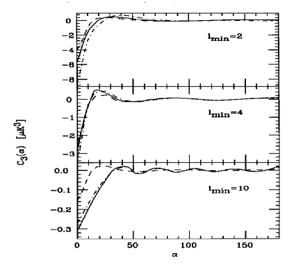
Figure 6.1: The collapsed three–point function ${\rm C}_{3}(\alpha)\equiv T_{0}^{3}\bigl{\langle}C_{3}(\alpha)\bigr{\rangle}$ (where $\bigl{\langle}C_{3}(\alpha)\bigr{\rangle}$ is given in the text), in $\mu K^{3}$ units, as predicted by the Rees–Sciama effect, vs. the angular scale $\alpha$. The dot–dashed line curves refer to the $n=0.7$ spectral index, the solid line ones to $n=1$ and the dashed line ones to $n=1.3$. The top, middle and bottom panels represent the cases $l_{min}=2,~{}4,~{}10$ respectively.

Figure 6.2 contains the corresponding plots for the rms collapsed three–point function obtained from our initially Gaussian fluctuation field, $\langle C_{3}^{2}(\alpha)\rangle_{Gauss}^{1/2}$.

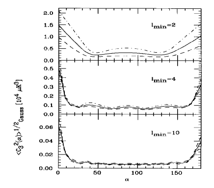
Figure 6.2: The rms collapsed three–point function $\langle{\rm C}_{3}^{2}(\alpha)\rangle^{1/2}_{Gauss}\equiv T_{0}^{3}\langle C_{3}^{2}(\alpha)\rangle^{1/2}_{Gauss}$ (where $\langle C_{3}^{2}(\alpha)\rangle^{1/2}_{Gauss}$ is given in the text), in $10^{4}~{}\mu K^{3}$ units, as arising from the cosmic variance of Gaussian fluctuations. Symbols are as in the previous figure. Note that the top, middle and bottom panels, representing the cases $l_{min}=2,~{}4,~{}10$ respectively, have different vertical scales.

So far we have assumed full–sky coverage; the effect of partial coverage, due to the cut at Galactic latitude $|b|<20^{\circ}$, increases the cosmic variance and can be approximately taken into account by multiplying it by a factor $1.56$ [Hinshaw et al., 1994]. An analytic estimate [Srednicki, 1993; Scott, Srednicki & White, 1994] gives a somewhat smaller value, 1.23. Note that the subtraction of low order multipoles leads to a strong decrease both in the signal and in the cosmic variance. For all considered multipole subtractions and angular separations, the expected signal stays typically three orders of magnitude below the cosmic variance, which makes the effect undetectable. The results are found to be weakly dependent on the considered spectral index. For comparison, the amplitude of the collapsed three–point function produced by non–linearities in the inflaton dynamics [see Gangui et al., 1994] is about a factor of ten smaller than that arising from the Rees–Sciama effect. We can also evaluate the skewness parameter ${\cal S}_{2}\equiv\langle(\Delta T/T)^{3}\rangle/\langle(\Delta T/T)^{2}\rangle^{2}$, which has the advantage of being normalisation (i.e., $Q_{rms-PS}$) independent for the considered effect (cf. §5.3); in the case, e.g., of only dipole subtraction and $n=1$, ${\cal S}_{2}\approx-5$. Note that, in the same case, the heuristic estimate by Luo & Schramm [1993] leads to ${\cal S}_{2}\approx 18$, while the method by Munshi et al. [1995] yielded ${\cal S}_{2}\approx-1$ (slight underestimate – now revised to ${\cal S}_{2}\approx-5$ ($-2$) with (without) $\theta_{FWHP}=10^{\circ}$ smoothing). The corresponding rms skewness parameter, arising from the cosmic variance of a scale–invariant Gaussian field, is ${\cal S}_{2}^{rms}\approx 1.3\times 10^{4}~{}(Q_{rms-PS}/19.5~{}\mu{\rm K})^{-1}$.

One may try to increase the amplitude of the signal–to–cosmic variance ratio, by referring to experimental settings, such as FIRS [e.g., Ganga et al., 1993] and Tenerife [e.g., Hancock et al., 1994], which are more sensitive to intermediate angular scales. However, the little increase of this ratio is not enough to make it detectable; furthermore, one has to bear in mind that the Tenerife measurement is further affected by a large sample variance.

Finally, let us stress that our calculations, reported in [Mollerach, Gangui, Lucchin & Matarrese, 1995], apply to measurements of CMB anisotropies on scales large enough to be unaffected by the Doppler peak. The possible extension of this effect to smaller scales is discussed by Munshi et al. [1995], who however argue that also on those scales the cosmic variance largely overcomes the intrinsic non–Gaussian signal.

Chapter 7 On the CMB kurtosis from cosmic strings

7.1 Introduction

We have seen in Chapter 2 how the strong link between cosmology and particle physics led to the generation of mainly two classes of theories which attempt to provide physically motivated solutions to the problem of the origin of structure in the universe. According to the one class of theories, based on inflation [e.g., Linde, 1990], primordial inhomogeneities in the energy density arose from zero–point quantum fluctuations of a scalar field during an epoch of superluminal expansion of the universe. These fluctuations may be shown to obey Gaussian statistics to a very high degree and to lead to an approximately scale invariant power spectrum of density perturbations. According to the second class of theories, those based on topological defects [e.g., Vilenkin & Shellard, 1994; Hindmarsh & Kibble, 1994], primordial fluctuations were produced by a superposition of seeds made of localised energy density trapped during a symmetry breaking phase transition in the early universe. Topological defects with linear geometry are known as cosmic strings and may be shown to be consistent with standard cosmology, unlike their pointlike (monopoles) and planar (domain walls) counterparts which require dilution by inflation to avoid overclosing the universe. Cosmic strings are predicted to form during a phase transition in the early universe by many but not all grand unified theories.

Cosmic strings can explain the formation of large scale filaments and sheets [Vachaspati, 1986; Stebbins et al., 1987; Perivolaropoulos et al., 1990; Vachaspati & Vilenkin, 1991; Vollick, 1992; Hara & Miyoshi, 1993], galaxy formation at epochs $z\sim 2-3$ [Brandenberger et al., 1987] and galactic magnetic fields [Vachaspati, 1992b]. They can also account for peculiar velocities on large scales [Vachaspati, 1992a; Perivolaropoulos & Vachaspati, 1994], and are consistent with the amplitude, spectral index [Bouchet et al., 1988; Bennett, Stebbins & Bouchet, 1992; Perivolaropoulos, 1993a; Hindmarsh, 1994] and the statistics [Gott et al., 1990; Perivolaropoulos, 1993b; Moessner et al., 1994; Coulson et al., 1994; Luo, 1994; Gangui & Perivolaropoulos, 1995] of the CMB anisotropies measured by COBE on angular scales of order $\theta\sim 10^{\circ}$. Strings may also leave their imprint on the CMB mainly in three different ways. The best studied mechanism for producing temperature fluctuations on the CMB by cosmic strings is the Kaiser–Stebbins effect [Kaiser & Stebbins, 1984; Gott, 1985]. According to this effect, moving long strings present between the time of last scattering $t_{ls}$ and today produce (due to their deficit angle [Vilenkin, 1981]) discontinuities in the CMB temperature between photons reaching the observer through opposite sides of the string. Other mechanisms through which cosmic strings may produce CMB fluctuations are based, e.g., on potential fluctuations on the last scattering surface, by inducing density and velocity fluctuations to the matter surrounding moving strings; and on the Doppler effect, by producing peculiar velocities in the ambient matter formed by the photon’s last scatterers.

It was recently shown [Perivolaropoulos, 1994] how, by superposing the effects of these three mechanisms at all times from $t_{ls}$ to today, the power spectrum of the total temperature perturbation may be obtained. It turns out that (assuming standard recombination) both Doppler and potential fluctuations at the last scattering surface dominate over post–recombination effects on angular scales below $2^{\circ}$. However this is not the case for very large scales (where we will be focusing in the present Chapter) and this justifies our neglecting the former two sources of CMB anisotropies. The main effect of these neglected perturbations is an increase of the Gaussian character of the fluctuations on small angular scales. Thus, in what follows we will be considering exclusively anisotropies generated through the Kaiser–Stebbins effect.

The main assumptions of the model were explained in [Perivolaropoulos, 1993a]. The magnitude of the discontinuity is proportional not only to the deficit angle but also to the string velocity $v_{s}$ and depends on the relative orientation between the unit vector along the string ${\hat{s}}$ and the unit photon wave–vector ${\hat{\gamma}}$. It is given by [Stebbins, 1988]

$${{\Delta T}\over T}=\pm 4\pi G\mu\gamma_{s}v_{s}\,{\hat{\gamma}}\cdot({\hat{v}_{s}}\times{\hat{s}}),$$ (7.1)

where $\gamma_{s}$ is the relativistic Lorentz factor and the sign changes when the string is crossed. Also, long strings within each horizon have random velocities, positions and orientations. In Eq. (7.1), $G$ is Newton’s constant and units are chosen such that $\hbar=c=1$, implying $G=m_{P}^{-2}$; $\mu\simeq m_{GUT}^{2}$ is the effective mass per unit length of the wiggly string. $G\mu\simeq 10^{-6}$ is needed for consistency of the string scenario with both a physically realisable GUT phase transition and a correct level of CMB anisotropies.

In what follows we will be mainly concerned with the computation of higher order correlation functions for CMB temperature anisotropies. In this Chapter, in addition to calculating the excess kurtosis parameter for the string–induced CMB temperature perturbations, we also show (with explicit formulae) how to estimate the intrinsic uncertainties with which the non–Gaussian signal ought to be confronted, when worked out at very large angular scales. Although the final result is somewhat disappointing (in the fact that the signal cannot be resolved) we think it is interesting to show explicit computations (even under simplifying assumptions within an analytic approach) of these string–induced higher order correlation functions. In the following section we show how to construct the general q–point function of CMB anisotropies at large angular scales produced through the Kaiser–Stebbins effect. Explicit calculations are performed for the four–point function and its zero–lag limit, the kurtosis. Next, we calculate the (cosmic) variance for the kurtosis assuming Gaussian statistics for arbitrary value of the spectral index and compare it with the string predicted value (§7.3). Finally, in §7.4 we briefly discuss our results.

7.2 The four–point temperature correlation function

We discretise the time between $t_{ls}$ and today by a set of $N$ Hubble time–steps $t_{i}$ such that $t_{i+1}=2\,t_{i}$, i.e., the horizon gets doubled in each time–step. For a redshift $z_{ls}\sim 1400$ we have $N\simeq\log_{2}[(1400)^{3/2}]\simeq 16$. In the frame of the multiple impulse approximation [Vachaspati, 1992a] the effect of the string network on a photon–beam is just the linear superposition of the individual effects, taking into account compensation [Traschen et al., 1986; Veeraraghavan & Stebbins, 1990; Magueijo, 1992], that is, only those strings within a horizon distance from the beam inflict perturbations to the photons. According to the previous description of the Kaiser–Stebbins effect, the total CMB temperature shift in the $\hat{\gamma}$ direction may be approximately written as the sum of all single impulses on the microwave photons caused by each of the strings, over all Hubble time–steps $N$ between the time of last scattering and today [Perivolaropoulos, 1993a]

$${\Delta T\over T}(\hat{\gamma})=4\pi G\mu\gamma_{s}v_{s}\sum_{n=1}^{N}\sum_{m=1}^{M}\beta^{mn}(\hat{\gamma}),$$ (7.2)

where $\beta^{mn}(\hat{\gamma})$ gives us information about the velocity $v^{mn}$ and orientation $s^{mn}$ of the $m$th string at the $n$th Hubble time–step and may be cast as $\beta^{mn}(\hat{\gamma})=\hat{\gamma}\cdot\hat{R}^{mn}$, with $\hat{R}^{mn}=v^{mn}\times s^{mn}=(\sin\theta^{mn}\cos\phi^{mn},\sin\theta^{mn}\sin\phi^{mn},\cos\theta^{mn})$ a unit vector whose direction varies randomly according to the also random orientations and velocities in the string network. In Eq. (7.2), $M$ denotes the mean number of strings per horizon scale, obtained from simulations [Allen & Shellard, 1990; Bennett & Bouchet, 1988] to be of order $M\sim 10$.

Given an arbitrary angle on the sky $\Delta\theta$, we will see now how to compute the number of perturbations (impulses) common to a pair of photon beams (see Figure 7.1). We are focusing here in the stringy–perturbations inflicted on photons after the time of last scattering, on their way to us. Recall we have discretised the time such that the horizon increases by a factor 2 with each time–step. Thus, at a particular step $p$ (with $1\leq p\leq N\simeq 16$) we have $t_{p}=2^{p}t_{ls}$. For a spatially flat, matter dominated universe ($a_{t}\equiv a(t)\propto t^{2/3}$) and in the small angle limit, we may write $\theta_{t_{p}}\simeq 1.5^{\circ}(z(t_{p})/1400)^{-1/2}$, for the apparent angular size of the horizon at $t_{p}$. Then, the ratio of the apparent horizon at time $t_{p}$ to that at last scattering is given by

$${\theta_{t_{p}}\over\theta_{ls}}\simeq\left({a_{t_{p}}\over a_{ls}}\right)^{1/2}=\left({t_{p}\over t_{ls}}\right)^{1/3}=2^{p/3}.$$ (7.3)

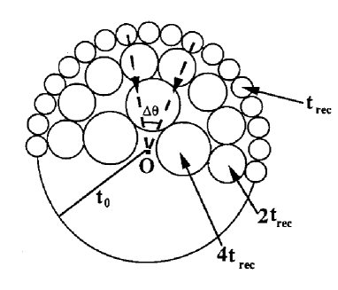
Figure 7.1: Two photon–beam paths separated by an angle $\Delta\theta$, starting off their trip at the time of last scattering (noted $t_{rec}$ in the plot) and being detected by an observer O at $t_{0}$. The horizon in three Hubble time–steps is shown. The effects of strings during the first two time–steps are uncorrelated for the particular angular beam separation shown.

Let us now take an arbitrary angle $\alpha_{12}$ on the sky. Consider a pair of photons with angular separation $\alpha_{12}=\arccos(\hat{\gamma}_{1}\!\cdot\!\hat{\gamma}_{2})$ greater than $\theta_{t_{p}}$, for a particular value of $p$ [here $\hat{\gamma}_{1}$ ($\hat{\gamma}_{2}$) is the line–of–sight direction of the first (second) photon]. Both of these photons will suffer temperature perturbations due to the presence of $\sim M$ strings per Hubble time–step. These perturbations, however, cannot be causally correlated at $t_{p}$, since the size of the causal regions surrounding each of these photons is smaller than the angle $\alpha_{12}$ between them. Thus, existing no overlapping of their horizons, each photon will be perturbed by different strings, and therefore the perturbations will be uncorrelated.

Given the angle $\alpha_{12}$ it is easy to compute the number of steps $N_{uncorr}$ during which the perturbations on these photons are uncorrelated: just substitute $\theta_{t_{p}}$ by $\alpha_{12}$ in Eq. (7.3) to get $N_{uncorr}(\alpha_{12})=3\log_{2}(\alpha_{12}/\theta_{ls})$, which is valid for $\alpha_{12}\geq\theta_{ls}\simeq 1.5^{\circ}$. Obviously, the larger the angular scale $\alpha_{12}$, the more steps $N_{uncorr}$ will be needed for the angular size of the horizon to overtake this scale. If we now define $\alpha_{12}^{\prime}\geq 0$ such that $\alpha_{12}=\alpha_{12}^{\prime}+\theta_{ls}$, subtract $N_{uncorr}$ from the maximum number of steps $N$ of the discretisation of the time along the photon path, and finally multiply the result by the scaling number of strings per Hubble time–step $M$, we get

$${\cal N}_{corr}(\alpha_{12})\equiv M[N-N_{uncorr}]=M[N-3\log_{2}(1+{\alpha_{12}\over\theta_{ls}})],$$ (7.4)

where ${\cal N}_{corr}(\alpha_{12})$ is the number of correlated ‘kicks’ inflicted on a pair of photons on a scale $\alpha_{12}$, after this scale has entered the horizon and up to the present epoch. In this equation, $\alpha_{12}\geq 0$ and primes were dropped. In other words: ${\cal N}_{corr}(\alpha_{12})$ counts the total number of correlated kicks onto the pair of photons after the time at which the angle $\alpha_{12}$ between their lines–of–sight fits in the horizon scale.

Much in the same way, kicks inflicted on three photon–beams will be uncorrelated at time $t_{p^{\prime}}$ if any one of the three angles between any two directions (say, $\alpha_{12}$, $\alpha_{23}$, $\alpha_{13}$) is greater than $\theta_{t_{p^{\prime}}}$, the size of the apparent horizon at time $t_{p^{\prime}}$. So, in this case, we will be summing (cf. Eq.(7.2)) over those Hubble time–steps $n$ greater than $p$, where $p$ ($>p^{\prime}$) is the time–step when the condition $\theta_{t_{p}}={\rm max}[\alpha_{12},\alpha_{23},\alpha_{13}]$ is satisfied. The same argument could be extended to any number of photon–beams (and therefore for the computation of the q–point function of temperature anisotropies).

Let us now study the correlations in temperature anisotropies and put the above considerations on more quantitative grounds, by writing the mean q–point correlation function. Using Eq. (7.2) we may express it as

$$\bigl{\langle}{{\Delta T}\over T}(\hat{\gamma}_{1})...{{\Delta T}\over T}(\hat{\gamma}_{q})\bigr{\rangle}=\xi^{q}\sum_{n_{1},...,n_{q}=1}^{N}\sum_{m_{1},...,m_{q}=1}^{M}\bigl{\langle}\beta_{1}^{m_{1}n_{1}}...\beta_{q}^{m_{q}n_{q}}\bigr{\rangle}$$ (7.5)

where $\hat{\gamma}_{1}...\hat{\gamma}_{q}$ are unit vectors denoting directions in the sky and where $\beta_{j}^{m_{j}n_{j}}={\hat{\gamma}_{j}}\cdot{\hat{R}^{m_{j}n_{j}}}$, with ${\hat{\gamma}_{j}}=(\sin\theta_{j}\cos\phi_{j},\sin\theta_{j}\sin\phi_{j},cos\theta_{j})$. In the previous equation we called $\xi\equiv 4\pi G\mu\gamma_{s}v_{s}$. We are here defining the ensemble average in the usual way; namely, $\bigl{\langle}{\Delta T\over T}(\hat{\gamma}_{1}){\Delta T\over T}(\hat{\gamma}_{2})\bigr{\rangle}$ represents the average of ${\Delta T\over T}(\hat{\gamma}_{1}){\Delta T\over T}(\hat{\gamma}_{2})$, for fixed directions ($\hat{\gamma}_{1}$, $\hat{\gamma}_{2}$) over a large number of realisations of the CMB sky. By assuming ergodicity, this is equivalent to performing a spatial average over the whole sky sphere, with fixed angle $\alpha_{12}=\arccos(\hat{\gamma}_{1}\!\cdot\!\hat{\gamma}_{2})$, for a single CMB realisation. Furthermore, we may supplement our definition with the property that also $\bigl{\langle}\cdot\bigr{\rangle}=0$ during those time–steps when the impulses on different photon–beams are uncorrelated. Thus, $\bigl{\langle}\cdot\bigr{\rangle}$ accounts also for compensation effects, according to which at sufficiently early times no string could have perturbed both photon–beams whose causal regions were much smaller than the angle between them. For simplicity we may always choose a coordinate system such that $\theta_{1}=0$, $\phi_{1}=0$ (i.e., $\hat{\gamma}_{1}$ lies on the $\hat{z}$ axis) and $\phi_{2}=\pi/2$. The seemingly complicated sum (7.5) is in practice fairly simple to calculate because of the large number of terms that vanish due to lack of correlation, after the average is taken. The calculation proceeds by first splitting the product $\beta_{1}^{m_{1}n_{1}}...\beta_{q}^{m_{q}n_{q}}$ into all possible sub–products that correspond to correlated kicks at each expansion time–step (i.e., $\beta^{m_{j}n_{j}}$’s with the same pair ($m_{j},n_{j}$) corresponding to the same string perturbing both beams), and then evaluating the ensemble average of each sub–product by integration over all directions of ${\hat{R}}^{m_{j}n_{j}}$. To illustrate this technique we evaluate the two–, three– and four–point functions below.

Let us start off with the two–point function. Having a correlated pair of beams in $\hat{\gamma}_{1}$ and $\hat{\gamma}_{2}$ directions from a particular time–step $p$ onwards means simply that $\hat{R}^{m_{1}n_{1}}=\hat{R}^{m_{2}n_{2}}\Leftrightarrow n\equiv n_{1}=n_{2}>p\,,\,m\equiv m_{1}=m_{2}$; otherwise the ${\hat{R}}^{m_{j}n_{j}}$’s remain uncorrelated and there is no contribution to the mean two–point function. Therefore we will have

$${\Delta T\over T}(\hat{\gamma}_{1}){\Delta T\over T}(\hat{\gamma}_{2})=\xi^{2}\sum_{n=p}^{N}\sum_{m=1}^{M}(\hat{\gamma}_{1}\cdot\hat{R}^{mn})(\hat{\gamma}_{2}\cdot\hat{R}^{mn}),$$ (7.6)

where we wrote just the correlated part on an angular scale $\alpha_{12}=\arccos(\hat{\gamma}_{1}\!\cdot\!\hat{\gamma}_{2})$. The uncorrelated part on this scale will vanish when performing the ensemble average $\bigl{\langle}\cdot\bigr{\rangle}$, as we explained before. Thus the mean two–point function may be written as

$$\bigl{\langle}{{\Delta T}\over T}({\hat{\gamma}_{1}}){{\Delta T}\over T}({\hat{\gamma}_{2}})\bigr{\rangle}=\xi^{2}\bigl{\langle}\beta_{1}\beta_{2}\bigr{\rangle}{\cal N}_{corr}(\alpha_{12}),$$ (7.7)

with ${\cal N}_{corr}(\alpha_{12})$ given in (7.4). Since we may always take

$$\beta_{1}=(0,0,1)\cdot{\hat{R}}~{}~{};~{}~{}\beta_{2}=(\sin\alpha_{12},0,\cos\alpha_{12})\cdot{\hat{R}}~{},$$ (7.8)

with ${\hat{R}}\equiv{\hat{R}}^{m_{1}n_{1}}=(\sin\theta\cos\phi,\sin\theta\sin\phi,cos\theta)$, $\bigl{\langle}{{\Delta T}\over T}({\hat{\gamma}_{1}}){{\Delta T}\over T}({\hat{\gamma}_{2}})\bigr{\rangle}$ may be calculated by integrating over $(\theta,\phi)$ and dividing by $4\pi$. The result is

$$\bigl{\langle}{{\Delta T}\over T}({\hat{\gamma}_{1}}){{\Delta T}\over T}({\hat{\gamma}_{2}})\bigr{\rangle}=\xi^{2}{{\cos\alpha_{12}}\over 3}{\cal N}_{corr}(\alpha_{12}),$$ (7.9)

which may be shown [Perivolaropoulos, 1993a] to lead to a slightly tilted scale invariant spectrum on large angular scales.

The three–point function may be obtained in a similar way. In our analytic approach however, the superimposed kernels of the distribution turn out to be symmetric with respect to positive and negative perturbations and therefore no mean value for the three–point correlation function arises (in particular also the skewness is zero). Similar conclusions were derived from exact lattice solutions to the Nambu equations, for string evolution and reconnection according to the Smith & Vilenkin [1987] scheme, adapted for evolving the network in an expanding universe [e.g., Coulson et al., 1994]. Notice also, that the effects of cosmic string loops that are ignored in the present study are expected to introduce a small skewness on scales of a few arcseconds or smaller (the typical angular scale of a string loop on the last scattering surface is a fraction of an arcsecond). On the other hand, the four–point function is easily found and a mean value for the excess kurtosis parameter [Gangui, 1995] may be predicted, as we show below.

In the case of the four–point function we could find terms where (for a particular time–step) the photon–beams in directions $\hat{\gamma}_{1}$, $\hat{\gamma}_{2}$ and $\hat{\gamma}_{3}$ are all correlated amongst themselves, but not with the beam $\hat{\gamma}_{4}$, which may be taken sufficiently far apart from the other three directions. In such a case we have

$$\bigl{\langle}{\Delta T\over T}(\hat{\gamma}_{1}){\Delta T\over T}(\hat{\gamma}_{2}){\Delta T\over T}(\hat{\gamma}_{3}){\Delta T\over T}(\hat{\gamma}_{4})\bigr{\rangle}\longrightarrow\bigl{\langle}{\Delta T\over T}(\hat{\gamma}_{1}){\Delta T\over T}(\hat{\gamma}_{2}){\Delta T\over T}(\hat{\gamma}_{3})\bigr{\rangle}\,\,\bigl{\langle}{\Delta T\over T}(\hat{\gamma}_{4})\bigr{\rangle}$$ (7.10)

and (cf. the discussion in the previous paragraph) this contribution vanishes. Another possible configuration we could encounter is the one in which the beams are correlated two by two, but no correlation exists between the pairs (for one particular time–step). This yields three distinct possible outcomes, e.g., $\bigl{\langle}{\Delta T\over T}(\hat{\gamma}_{1}){\Delta T\over T}(\hat{\gamma}_{2})\bigr{\rangle}\,\bigl{\langle}{\Delta T\over T}(\hat{\gamma}_{3}){\Delta T\over T}(\hat{\gamma}_{4})\bigr{\rangle}$, and the other two obvious combinations. The last possibility is having all four photon–beams fully correlated amongst themselves and this yields $\bigl{\langle}{\Delta T\over T}(\hat{\gamma}_{1}){\Delta T\over T}(\hat{\gamma}_{2}){\Delta T\over T}(\hat{\gamma}_{3}){\Delta T\over T}(\hat{\gamma}_{4})\bigr{\rangle}_{c}$, where the subscript $c$ stands for the connected part.

In a way completely analogous to that for the two–point function, the correlated part for the combination of four beams gives

$${\Delta T\over T}(\hat{\gamma}_{1}){\Delta T\over T}(\hat{\gamma}_{2}){\Delta T\over T}(\hat{\gamma}_{3}){\Delta T\over T}(\hat{\gamma}_{4})=\xi^{4}\sum_{n=p}^{N}\sum_{m=1}^{M}(\hat{\gamma}_{1}\!\cdot\!\hat{R}^{mn})(\hat{\gamma}_{2}\!\cdot\!\hat{R}^{mn})(\hat{\gamma}_{3}\!\cdot\!\hat{R}^{mn})(\hat{\gamma}_{4}\!\cdot\!\hat{R}^{mn})$$ (7.11)

Now we are ready to write the full mean four–point function as

$$\bigl{\langle}{\Delta T\over T}(\hat{\gamma}_{1}){\Delta T\over T}(\hat{\gamma}_{2}){\Delta T\over T}(\hat{\gamma}_{3}){\Delta T\over T}(\hat{\gamma}_{4})\bigr{\rangle}$$ (7.12)

$$=\!\!\left[\!\bigl{\langle}{\Delta T\over T}(\hat{\gamma}_{1}){\Delta T\over T}(\hat{\gamma}_{2})\bigr{\rangle}\bigl{\langle}{\Delta T\over T}(\hat{\gamma}_{3}){\Delta T\over T}(\hat{\gamma}_{4})\bigr{\rangle}\!+\!2{\rm terms}\right]\!\!+\!\!\bigl{\langle}{\Delta T\over T}(\hat{\gamma}_{1}){\Delta T\over T}(\hat{\gamma}_{2}){\Delta T\over T}(\hat{\gamma}_{3}){\Delta T\over T}(\hat{\gamma}_{4})\bigr{\rangle}_{c}$$

$$=3\left[{1\over 3}\xi^{2}{\cal N}_{corr}(\theta)\cos(\theta)\right]^{2}+\bigl{\langle}{\Delta T\over T}(\hat{\gamma}_{1}){\Delta T\over T}(\hat{\gamma}_{2}){\Delta T\over T}(\hat{\gamma}_{3}){\Delta T\over T}(\hat{\gamma}_{4})\bigr{\rangle}_{c}$$

where for simplicity we wrote this equation using the same scale $\theta$ for all directions on the sky (first term after the equality sign); after all, we will be interested in the zero–lag limit, in which case we will have $\theta\to 0$. By using Mathematica [Wolfram, 1991] it is simple to find that the second term includes just the sum of twenty–one combinations of trigonometric functions depending on $\theta_{i},\phi_{i}$, with $i=1,2,3,4$, the spherical angles for the directions $\hat{\gamma}_{i}$ on the sky (cf. Eq. (7.11)). These terms are the only ones which contribute non–vanishingly after the integration over the angles $\theta^{mn},\phi^{mn}$ is performed (assuming ergodicity).

When we take the zero–lag limit (i.e., aiming for the kurtosis) the above expression gets largely simplified. After normalizing by the squared of the variance $\sigma^{4}=[{1\over 3}\xi^{2}{\cal N}_{corr}(0)]^{2}$ and subtracting the disconnected part we get the excess kurtosis parameter

$${\cal K}={1\over\sigma^{4}}\bigl{\langle}{\Delta T\over T}^{4}(\hat{\gamma}_{1})\bigr{\rangle}-3\simeq 1.125\left[{10\over M}\right]\times 10^{-2}.$$ (7.13)

Note that for values of the scaling solution $M$ increasing (large number of seeds) the actually small non–Gaussian signal ${\cal K}$ gets further depressed, as it could be expected from the Central Limit Theorem.

7.3 The r.m.s. excess kurtosis of a Gaussian field

The previous section was devoted to the computation of ${\cal K}$, the excess kurtosis parameter, as predicted by a simple analytic model in the framework of the cosmic string scenario. We might ask whether this particular non–Gaussian signal has any chance of actually being unveiled by current anisotropy experiments. Needless to say, this could provide a significant probe of the structure of the relic radiation, and furthermore give us a hint on the possible sources of primordial perturbations.

However, as it was realised some time ago [Scaramella & Vittorio, 1991; see also e.g., Abbott & Wise, 1984, Srednicki, 1993], the mere detection of a non–zero higher order correlation function (e.g., the four–point function) or its zero–lag limit (e.g., the kurtosis) cannot be directly interpreted as a signal for intrinsically non–Gaussian perturbations. In order to tell whether or not a particular measured value for the kurtosis constitutes a significant evidence of a departure from Gaussian statistics, we need to know the amplitude of the non–Gaussian pattern produced by a Gaussian perturbation field. Namely, we need to know the rms excess kurtosis of a Gaussian field.

Let us begin with some basics. Let us denote the kurtosis $K\equiv\int{d\Omega_{\hat{\gamma}}\over 4\pi}{\Delta T\over T}^{4}(\hat{\gamma})$ and assume that the underlying statistics is Gaussian, namely, that the multipole coefficients $a_{\ell}^{m}$ are Gaussian distributed. Thus, the ensemble average for the kurtosis is given by the well–known formula: $\bigl{\langle}K\bigr{\rangle}=3\sigma^{4}$, where $\sigma^{2}$ is the mean two–point function at zero–lag, i.e., the CMB variance as given by

$$\sigma^{2}\equiv\bigl{\langle}C_{2}(0)\bigr{\rangle}={1\over 4\pi}\sum_{\ell}(2\ell+1){\cal C}_{\ell}{\cal W}^{2}_{\ell}~{},$$ (7.14)

where the ${\cal C}_{\ell}$ coefficients are also dependent on the value for the primordial spectral index of density fluctuations $n$ and are given by the usual expression in terms of Gamma functions, cf. Eq. (4.20). In the previous expression ${\cal W}_{\ell}$ represents the window function of the specific experiment. In the particular case of the COBE–DMR experimental setup we have, for $\ell\geq 2$, ${\cal W}_{\ell}\simeq\exp\left[-{\textstyle{1\over 2}}\ell({\ell}+1)(3.2^{\circ})^{2}\right]$, where $3.2^{\circ}$ is the dispersion of the antenna–beam profile.

However, $\bigl{\langle}K\bigr{\rangle}$ is just the mean value of the distribution and therefore we cannot know its real value but within some error bars. In order to find out how probable it is to get this value after a set of experiments (observations) is performed, we need to know the variance of the distribution for $K$. In other words, we ought to know how peaked the distribution is around its mean value $\bigl{\langle}K\bigr{\rangle}$. The width of the distribution is commonly parameterised by what is called the cosmic variance of the kurtosis: $\sigma_{CV}^{2}=\bigl{\langle}K^{2}\bigr{\rangle}-\bigl{\langle}K\bigr{\rangle}^{2}$. It is precisely this quantity what attaches theoretical error bars to the actual value for the kurtosis. Therefore, we may heuristically express the effect of $\sigma_{CV}^{2}$ on $K$ as follows: $K\simeq\bigl{\langle}K\bigr{\rangle}\pm\sigma_{CV}$, at one sigma level (a good approximation in the case of a narrow peak). Rearranging factors we may write this expression in a way convenient for comparing it with ${\cal K}$: ${\cal K}_{CV}=K/\sigma^{4}-3\simeq\pm\sigma_{CV}/\sigma^{4}$, where ${\cal K}_{CV}$ is the excess kurtosis parameter (assuming Gaussian statistics) purely due to the cosmic variance. Not only is ${\cal K}_{CV}$ in general non–zero, but its magnitude increases with the theoretical uncertainty $\sigma_{CV}$. This gives a fundamental threshold that must be overcome by any measurable kurtosis parameter. Namely, unless our predicted value for ${\cal K}$ exceeds ${\cal K}_{CV}$ we will not be able to tell confidently that any measured value of ${\cal K}$ is due to string–induced non–Gaussianities.

Let us now compute the cosmic variance of the kurtosis explicitly. We begin by calculating $\bigl{\langle}K^{2}\bigr{\rangle}$ as follows

$$\bigl{\langle}K^{2}\bigr{\rangle}=\int{d\Omega_{\hat{\gamma}_{1}}\over 4\pi}\int{d\Omega_{\hat{\gamma}_{2}}\over 4\pi}\bigl{\langle}{\Delta T\over T}^{4}(\hat{\gamma}_{1}){\Delta T\over T}^{4}(\hat{\gamma}_{2})\bigr{\rangle}.$$ (7.15)

By assuming Gaussian statistics for the temperature perturbations ${\Delta T\over T}(\hat{\gamma})$ we may make use of standard combinatoric relations, and get

$$\bigl{\langle}{\Delta T\over T}^{4}(\hat{\gamma}_{1}){\Delta T\over T}^{4}(\hat{\gamma}_{2})\bigr{\rangle}=\,9\,\bigl{\langle}{\Delta T\over T}^{2}(\hat{\gamma}_{1})\bigr{\rangle}^{2}\bigl{\langle}{\Delta T\over T}^{2}(\hat{\gamma}_{2})\bigr{\rangle}^{2}$$ (7.16)

$$+\,72\,\bigl{\langle}{\Delta T\over T}^{2}(\hat{\gamma}_{1})\bigr{\rangle}\bigl{\langle}{\Delta T\over T}^{2}(\hat{\gamma}_{2})\bigr{\rangle}\bigl{\langle}{\Delta T\over T}(\hat{\gamma}_{1}){\Delta T\over T}(\hat{\gamma}_{2})\bigr{\rangle}^{2}+\,24\,\bigl{\langle}{\Delta T\over T}(\hat{\gamma}_{1}){\Delta T\over T}(\hat{\gamma}_{2})\bigr{\rangle}^{4}.$$

As we know, the ensemble averages are rotationally invariant and therefore $\bigl{\langle}{\Delta T\over T}^{2}(\hat{\gamma}_{1})\bigr{\rangle}=\bigl{\langle}C_{2}(0)\bigr{\rangle}\equiv\sigma^{2}$ is independent of the direction $\hat{\gamma}_{1}$. Plug this last equation into Eq. (7.15) and we get

$$\bigl{\langle}K^{2}\bigr{\rangle}=9\sigma^{8}+36\sigma^{4}\int^{1}_{-1}d\cos\alpha\,\bigl{\langle}C_{2}(\alpha)\bigr{\rangle}^{2}+12\int^{1}_{-1}d\cos\alpha\,\bigl{\langle}C_{2}(\alpha)\bigr{\rangle}^{4}.$$ (7.17)

The above integrals may be solved numerically. Then, using this result in the expression for $\sigma_{CV}^{2}$ we get ${\cal K}_{CV}$, the value for the excess kurtosis parameter of a Gaussian field.

It is also instructive to look at Eq. (7.17) in some more detail, so that the actual dependence on the spectral index becomes clear. By expanding the mean two–point correlation functions within this expression in terms of spherical harmonics and after some long but otherwise straightforward algebra we find

$${\cal K}_{CV}=\left[\,72\,{\sum_{\ell}(2\ell+1){\cal C}_{\ell}^{2}{\cal W}_{\ell}^{4}\over[\sum_{\ell}(2\ell+1){\cal C}_{\ell}{\cal W}_{\ell}^{2}]^{2}}\right.$$ (7.18)

$$+\,\left.24\,{\{\prod_{i=1}^{4}\sum_{\ell_{i}}\sum_{m_{i}=-\ell_{i}}^{\ell_{i}}{\cal C}_{\ell_{i}}{\cal W}_{\ell_{i}}^{2}\}\left(\sum_{L}4\pi\,\bar{\cal H}_{\ell_{1},\,\,\ell_{2}\,,\,\,\,\,L}^{m_{1},m_{2},m_{3}+m_{4}}\bar{\cal H}_{\ell_{3},\,\,\ell_{4}\,,\,\,\,\,\,\,L}^{m_{3},m_{4},-m_{3}-m_{4}}\right)^{2}\over[\sum_{\ell}(2\ell+1){\cal C}_{\ell}{\cal W}_{\ell}^{2}]^{4}}\right]^{1/2}$$

where the coefficients $\bar{\cal H}_{\ell_{1},\,\ell_{2},\,\ell_{3}}^{m_{1},m_{2},m_{3}}\equiv\int d\Omega_{\hat{\gamma}}{Y_{\ell_{1}}^{m_{1}}}(\hat{\gamma})Y_{\ell_{2}}^{m_{2}}(\hat{\gamma})Y_{\ell_{3}}^{m_{3}}(\hat{\gamma})$ are those defined previously in Eq. (4.16). In the above equation the $n$–dependence is hidden inside the multipole coefficients ${\cal C}_{\ell}$ (cf. Eq.(4.20)).

Eq. (7.18) shows an analytic expression for computing ${\cal K}_{CV}$ which, in turn, represents a fundamental threshold for any given non–Gaussian signal. For interesting values of the spectral index (say, between $0.8\mathrel{\raise 1.29167pt\hbox{$<$\kern-7.5pt\lower 4.30554pt\hbox{$\sim$}}}n\mathrel{\raise 1.29167pt\hbox{$<$\kern-7.5pt\lower 4.30554pt\hbox{$\sim$}}}1.3$) we find no important variation in ${\cal K}_{CV}$, being its value consistent with the Monte–Carlo simulations performed by Scaramella & Vittorio [1991]. These authors concentrated on a Harrison–Zel’dovich spectrum, considered also the quadrupole contribution and took a slightly different dispersion width for the window function ($3.0^{\circ}$ in their simulations).

We solved Eq. (7.18) numerically. We subtracted the quadrupole contribution and performed the sums up to a $\ell_{max}=15$; the exponential suppression of the ${\cal W}_{\ell}$ window functions makes higher $\ell$ contribution to the sums negligible. Our analytic analysis expresses ${\cal K}_{CV}$ as a ratio of averages, rather than the average of a ratio as in [Scaramella & Vittorio, 1991], and therefore exact agreement between their and our result should not be expected. Nevertheless, we get the same order of magnitude for spectral index $n=1$. We also checked that a different $n$ does not change very much the value of ${\cal K}_{CV}$. We explored the cosmologically interesting range $0.8\leq n\leq 1.3$. In Figure 7.2 we plot ${\cal K}_{CV}$ versus the spectral index $n$, for $\ell_{max}=15$ and quadrupole contribution subtracted; the inclusion of the quadrupole in our results would do no more than slightly rise the whole set of points. This is not a new feature and simply reflects the intrinsic theoretical uncertainty of the lowest order multipoles.

Figure 7.2: Excess Kurtosis parameter of a Gaussian temperature fluctuation field as function of the spectral index; $\ell_{max}=15$ and the quadrupole contribution is subtracted.

Note the small rate of variation of ${\cal K}_{CV}$ with $n$ and that, as expected, ${\cal K}_{CV}$ takes larger values for smaller spectral indexes. This is clearly due to the fact that a small $n$ generates more power on large scales (i.e., small $\ell$), and precisely these scales are the ones that contribute the most to the cosmic variance of the kurtosis field.

7.4 Discussion

In the foregoing sections we showed how to implement the multiple impulse approximation for perturbations on a photon beam (stemming from the effect of the cosmic string network) in the actual construction of higher order correlations for the CMB anisotropies. We then focused on the four–point function and on the excess kurtosis parameter, finding for the latter a value ${\cal K}\sim 10^{-2}$.

We also found explicit formulae for calculating the rms excess kurtosis ${\cal K}_{CV}$ predicted to exist even for a Gaussian underlying field, and showed its dependence on the primordial spectral index of density fluctuations. This constitutes the main source of theoretical uncertainty at large angular scales, but not the only one: also the ‘sample variance’ [e.g., Scott et al., 1994] makes the signal hard to detect, since we should note that no complete sampling of the CMB sky is available, not even the COBE one, where galactic latitudes $|b|<20^{\circ}$ are cut out from the maps. These uncertainties completely hide the cosmic string signature: this is clearly seen from the results of §7.3, where it was shown that ${\cal K}_{CV}$ is two orders of magnitude larger than ${\cal K}$. The results of our analytic approach presented in §7.2 fully agree with those of [Coulson et al., 1994], where they found little evidence for non–Gaussianity in their simulated CMB maps, for a variety of smoothing angles. We conclude therefore that statistical effects of the kind just mentioned would be the most probable responsible of any kurtosis signal detected on COBE scales. The results presented in this Chapter have been published in [Gangui & Perivolaropoulos, 1995].

Chapter 8 Analytic modeling of textures

The analytic modeling of topological defects, like cosmic strings and textures, captures the essential features of their cosmological predictions. Analytic models are complementary to full numerical simulations of defect evolution and CMB temperature anisotropy generation, and they rely on these simulations for fixing some free parameters present in the models. However, large–scale anisotropies alone can only very barely discriminate between competing models of structure formation. In the present Chapter we include work in progress towards studying to what extent CMB non–Gaussian features further constrain topological defects models. We derive an analytic expression for the collapsed three–point correlation function in the CMB temperature anisotropies for textures, as well as for the rms collapsed three–point function (cosmic variance) associated with it. Applying our results to the COBE–DMR two–year data, preliminary estimates seem to indicate that the CMB non–Gaussianities predicted by this model are consistent with the theoretical uncertainties present in the maps, and therefore large scale anisotropies alone can not place further constraints on these models.

8.1 Introduction

One of the most compelling issues calling for thorough study regards the possibility of discriminating the real source of density perturbations leading to large–scale structure formation. Competing models are inflationary scenarios and topological defects (cf. Chapter 2), these latter formed as the consequence of a symmetry breaking phase transition in the early evolution of our universe.

The CMB radiation carries a valuable information of that early epoch when matter and photons were tightly coupled. A useful way of trying to discriminate between models is given by the structure in the relic radiation predicted by them. However, production of anisotropy maps from numerical simulations of the ‘defect’ field equations turns out to be a fabulous problem, and therefore some analytic insight is desirable. This is the reason why people turned to consider analytic (although simplified) models for anisotropy generation by defects, wherein the physics is more transparent and computations can be pursued straightforwardly [Perivolaropoulos, 1993; Magueijo, 1995; Gangui & Perivolaropoulos, 1995]. Although it is clear that full–range numerical simulations will have the last word regarding these and other observable signatures of defects, in the meantime progress with these simplified models will hint many of their important features.

Defect induced large–scale structure formation has been well studied recently [see, e.g., Vilenkin & Shellard, 1994; Pen et al., 1994] and their predictions confront successfully against a large bulk of observations. The amplitude of the anisotropies is directly related to the symmetry breaking energy scale, and normalisation to the COBE–DMR detection makes these seeds compatible with a physically realisable GUT phase transition.

However, more and valuable information can be readily extracted from the CMB maps. Recently Hinshaw et al. [1995] analysed the two–year COBE–DMR data and found evidence for a departure from Gaussian statistics, although consistent with the level of cosmic variance. Many are the models wherein non–Gaussian features can arise: in non–standard inflationary models, for example, primordial non–Gaussian features are easily generated [Falk et al., 1994; Gangui et al., 1994; Gangui, 1994; see also Chapter 5]. Furthermore, the post recombination mildly non–linear evolution of perturbations also predicts a non–Gaussian signature through the integrated Sachs–Wolfe effect [Luo & Schramm, 1993; Munshi et al., 1995; Mollerach et al., 1995; see also Chapter 6]. Here we will focus on the three–point correlation function of the CMB anisotropies. In particular, it turns out that a useful tool to quantify the departure from Gaussian statistics is given by the collapsed three–point function (cf. §4.3), and we will work exclusively with this latter in the present Chapter.

One might think that, due to the high level of theoretical noise inherent to the lowest order multipoles probed by COBE, very little can be said regarding non–Gaussian features in the CMB radiation on large scales. However, based on the analysis of the equilateral and collapsed three–point functions, Hinshaw et al. [1995] were able to rule out the primordial isocurvature baryon (PIB) power–law inflationary model considered by Yamamoto & Sasaki [1994]: in this model the predicted mean skewness vanishes and the rms skewness (cosmic variance) is several orders of magnitude below the corresponding level for standard adiabatic models. These authors suggest that the cosmic variance of the full three–point function would be tiny as well. This would make the theoretical error bars for the three–point function predicted by this PIB model even smaller that the actual data from the maps, hence running into conflict with the result of the COBE–DMR analysis.

Likewise, it is interesting to check whether the non–Gaussian signatures predicted by some recently proposed analytic defect models are in agreement with the analyses of the maps, and if not what the constraints are. This is the main aim of the present study, which, we reiterate, is in progress [70]. Let us now give a couple of definitions to set up the basic framework.

The three–point correlation function for points at three arbitrary angular separations $\alpha$, $\beta$ and $\gamma$ is given by the average product of temperature fluctuations in all possible three directions with those angular separations among them. The general expression is given in Eq. (4.14). Here, for simplicity, we will restrict ourselves to the collapsed case, corresponding to the choice $\alpha=\beta$ and $\gamma=0$ (one of the cases analysed for the COBE–DMR data by Hinshaw et al. [1994, 1995]). The collapsed three–point correlation function of the CMB is given by

$$C_{3}(\alpha)\equiv\int{d\Omega_{\hat{\gamma}_{1}}\over 4\pi}\int{d\Omega_{\hat{\gamma}_{2}}\over 2\pi}{\Delta T\over T}(\hat{\gamma}_{1}){\Delta T\over T}^{2}(\hat{\gamma}_{2})\delta(\hat{\gamma}_{1}\cdot\hat{\gamma}_{2}-\cos\alpha).$$ (8.1)

For $\alpha=0$, we recover the well–known expression for the skewness, $C_{3}(0)$. By expanding the temperature fluctuations in spherical harmonics ${\Delta T\over T}(\hat{\gamma})=\sum_{\ell,m}a_{\ell}^{m}Y_{\ell}^{m}(\hat{\gamma})$, we can write the collapsed three–point function as

$$C_{3}(\alpha)={\textstyle{1\over 4\pi}}\sum_{\ell_{1},\ell_{2},\ell_{3},m_{1},m_{2},m_{3}}P_{\ell_{1}}(\cos\alpha)a_{\ell_{1}}^{m_{1}}a_{\ell_{2}}^{m_{2}}a_{\ell_{3}}^{m_{3}}{\cal W}_{\ell_{1}}{\cal W}_{\ell_{2}}{\cal W}_{\ell_{3}}\bar{\cal H}_{\ell_{1}\ell_{2}\ell_{3}}^{m_{1}m_{2}m_{3}}~{},$$ (8.2)

where as usual ${\cal W_{\ell}}$ represents the window function of the particular experiment and we use the notation of Eq. (4.16).

Predictions for different models usually come as expressions for the angular bispectrum $\bigl{\langle}a_{\ell_{1}}^{m_{1}}a_{\ell_{2}}^{m_{2}}a_{\ell_{3}}^{m_{3}}\bigr{\rangle}$. As we saw in Chapter 7, within the analytic model for cosmic strings considered there, the bispectrum simply vanishes, and so does the three–point correlation function. In that case we are left just with the amplitude of the rms collapsed three–point function. For textures the situation is different, and it is one of the aims of the present study to show the variation of the collapsed function with the angle separation, as well as that of the rms collapsed three–point function.

8.2 Texture–spot statistics

One of the most serious complications in predicting CMB fluctuations in defect theories is the necessity of evolving the simulations over a large number of expansion times. Scaling helps in simplifying this issue in that if the defect is assumed to scale (and textures do scale) then the defect network looks statistically the same at any time, once its characteristic length is normalised to the horizon. Then, by dividing the sky cone into cells corresponding to expansion times and horizon volumes, one can restrict the study to the CMB pattern induced in horizon–size boxes during one Hubble time. Such studies have been performed by, e.g., Borrill et al. [1994] and Durrer et al. [1994]; in the latter paper, in particular, a ‘scaling–spot–throwing’ process was implemented numerically, with CMB spots derived from a self–similar and spherically symmetric model of texture collapses [Turok & Spergel, 1990; Notzold, 1991; see also §2.2].

The implementation (within the texture scenario) of an analytic approach for the computation of the multipole coefficients ${\cal C}_{\ell}$ and the full two–point function, as well as for their cosmic variances, was performed in [Magueijo, 1995]. The model allows to study texture–induced spots of arbitrary shapes and relies on a hand–full of ‘free’ parameters to be specified by numerical simulations, like the number density of spots, ${\bf n}$, the scaling size, $d_{s}$, and the brightness factor of the particular spot, $a_{n}$, which tells us about its temperature relative to the mean sky temperature (in particular, whether it is a hot or a cold spot). In the following we will briefly review the necessary basic features of the model and then move on directly to the specific study of interest to us, namely the collapsed three–point function predicted by the model, and its cosmic variance. We make a short discussion at the end where we summarise what was found so far.

Let us start off discussing the spots statistics. By dividing the whole volume in boxes of surface $dS$ and thickness $d\ell$ we may write the volume probability density of spot generation in the sky as follows

$$dP={{\bf n}\over H^{-4}}dSd\ell dt~{},$$ (8.3)

where ${\bf n}$ is the mean number of CMB spots expected in a horizon–size box volume and in a Hubble time. Now, we are interested in a two dimensional distribution of spots (since observations map the two dimensional sky sphere), and thus we may integrate the thickness $d\ell$ in an interval of order $H^{-1}$ to get the surface probability density

$$dP\simeq{{\bf n}\over H^{-3}}dSdt~{}.$$ (8.4)

Taking into account the expansion of the universe we may express $dS=r^{2}(t)d\Omega$, with $r(t)=3t((t_{0}/t)^{1/3}-1)$, where $t$ denotes proper time and $t_{0}$ stands for its value today.

We discretise the time between last scattering, $t_{ls}$, and today by a set of Hubble time–steps $t_{n}$ such that $t_{n+1}=2\,t_{n}$, i.e., the horizon gets doubled in each time–step. Thus, it turns out to be convenient to change time variable to $y_{n}(t_{n})\equiv\log_{2}(t_{0}/t_{n})$. For a redshift $z_{ls}\sim 1400$ we have $y_{ls}\simeq\log_{2}[(1400)^{3/2}]\simeq 16$. In terms of $y_{n}$ the surface probability density may be cast as

$$dP=N(y_{n})dyd\Omega,$$ (8.5)

with

$$N(y_{n})=-{8{\bf n}\ln(2)\over 3}\left(2^{y_{n}/3}-1\right)^{2}~{}.$$ (8.6)

Within the model, CMB anisotropies arise from texture–produced spots in the sky. Thus, we may also express the anisotropies in terms of the profiles $W_{n}$ of these spots, generated at time $y_{n}$, as follows: ${\Delta T\over T}=\sum_{n}a_{n}W_{n}(\theta_{n},y_{n})$. Here, $a_{n}$ characterises the brightness of the hot/cold $n$–th spot [Magueijo, 1995] and is interpreted as a random variable: it is non–Gaussian distributed and its possible mean values are to be computed from numerical simulations [e.g., Borrill et al., 1994]. $\theta_{n}$ is the angle subtended by a scale characterising the size of the spots in the particular Hubble time step $y_{n}$, as measured by a given observer.

The non–linear evolution of the global scalar field responsible for texture formation is the source of the CMB anisotropies. As long as the characteristic length scale of these defects is larger than the size of the horizon the gradients of the field are frozen in and cannot affect the surrounding matter components. However, when the size of the texture becomes comparable to the Hubble radius (this latter growing linearly with cosmic time), microphysical processes can ‘push’ the global fields so that they finally acquire trivial field configurations, reduce their energy (which is radiated away as Goldstone bosons) and, in those cases where the field was wounded in knots, they unwind. In so doing they generate perturbations in the metric of spacetime and hence affect also the photon geodesics. These unwinding events are mainly characterised by one length scale, that of the horizon at the moment of collapse, implying that the outcome perturbations arise at a fixed rate per horizon volume and Hubble time.

It is this ‘scaling’ behaviour what makes texture seeds a viable model for structure formation; being a generic outcome of any symmetry breaking phase transition involving a non–Abelian GUT group, if they did not collapse not only would they be the storage of huge amounts of energy (e.g., in the form of gradients of the global fields) but they would also produce too much anisotropy in the CMB and would therefore be cosmologically intolerable. It is therefore natural to expect a similar scaling for the pattern of the spots they produce. A spot appearing at time $y_{n}$ has typically a size $\theta^{s}(y_{n})\simeq d_{s}~{}\theta^{hor}(y_{n})$, with $\theta^{hor}(y_{n})$ the angular size of the horizon at $y_{n}$, and where

$$\theta^{s}(y_{n})=\arcsin\left({d_{s}H^{-1}\over r(t)}\right)=\arcsin\left({0.5d_{s}\over 2^{y_{n}/3}-1}\right)~{}.$$ (8.7)

Spot anisotropies are generated by causal seeds, and therefore their angular size cannot exceed the size of the horizon at that time; thus we have $d_{s}\mathrel{\raise 1.29167pt\hbox{$<$\kern-7.5pt\lower 4.30554pt\hbox{$\sim$}}}1$. The scaling hypothesis implies that the profiles satisfy $W_{n}(\theta_{n},y_{n})=W_{n}(\theta_{n}/\theta^{s}(y_{n}))$.

Combining both previous expansions for ${\Delta T\over T}$ we easily find the expression for the multipole coefficients $a_{\ell}^{m}$ in terms of the brightness and the profile of the spots

$$a_{\ell}^{m}={4\pi\over 2\ell+1}\sum_{n}a_{n}W_{n}^{\ell}{Y_{\ell}^{m}}^{*}(\hat{\gamma}_{n})~{},$$ (8.8)

where

$$W_{n}^{\ell}={2\ell+1\over 2}\int_{-1}^{1}W_{n}(x)P_{\ell}(x)dx~{}.$$ (8.9)

8.3 Spot correlations

Having derived the $a_{\ell}^{m}$ coefficients of the expansion of ${\Delta T\over T}$ in spherical harmonics, we are able now to compute correlations, namely the angular spectrum and angular bispectrum predicted within this analytic model. From Eq. (8.8) we may easily calculate the quantity

$${1\over 2\ell+1}\sum_{m=-\ell}^{\ell}|a_{\ell}^{m}|^{2}={4\pi\over(2\ell+1)^{2}}\sum_{nn^{\prime}}a_{n}a_{n^{\prime}}W_{n}^{\ell}W_{n^{\prime}}^{\ell}P_{\ell}(\hat{\gamma}_{n}\cdot\hat{\gamma}_{n^{\prime}})~{}.$$ (8.10)

Now let us compute ensemble averages $\bigl{\langle}\cdot\bigr{\rangle}$. Any two texture–spots located at different $\hat{\gamma}_{n}$’s are uncorrelated, hence we have

$$\bigl{\langle}a_{n}a_{n^{\prime}}W_{n}^{\ell}W_{n^{\prime}}^{\ell}P_{\ell}(\hat{\gamma}_{n}\cdot\hat{\gamma}_{n^{\prime}})\bigr{\rangle}=\delta_{nn^{\prime}}a_{n}^{2}\left(W_{n}^{\ell}\right)^{2}~{}.$$ (8.11)

In the present model, due to this lack of correlation, the angular part of the surface probability density (cf. Eq. (8.5)) yields just a kronecker delta and disappears from the expression of the angular power spectrum $\bigl{\langle}|a_{\ell}^{m}|^{2}\bigr{\rangle}={\cal C}_{\ell}$. In fact, from Eqs. (8.10) and (8.11) we get

$${\cal C}_{\ell}={4\pi\over(2\ell+1)^{2}}\sum_{n}a_{n}^{2}\left(W_{n}^{\ell}\right)^{2}~{}.$$ (8.12)

The cumulative effect of the different spots on the ${\cal C}_{\ell}$’s (as reflected from the profiles $W_{n}^{\ell}$) is computed from the surface probability density (cf. Eq. (8.5)). Going to the continuous limit in the time variable $y$ the above equation may be cast as

$${\cal C}_{\ell}=\bigl{\langle}a^{2}\bigr{\rangle}\left({4\pi\over 2\ell+1}\right)^{2}{\cal I}_{2}^{\ell\ell}$$ (8.13)

where we defined

$${\cal I}_{D}^{\ell_{1}\ldots\ell_{D}}\equiv\int dyN(y)W^{\ell_{1}}(y)\ldots W^{\ell_{D}}(y)~{}.$$ (8.14)

In these equations and hereafter we drop the _n subindex and consider $y$ in the continuous limit. $\bigl{\langle}a^{2}\bigr{\rangle}$ in Eq. (8.13) is the mean squared value of the spot brightness, to be computed from the distribution {$a_{n}$} resulting from simulations.

8.4 Textures and the three–point function

Let us now compute the angular bispectrum. Following the same steps as in the previous section we may express it as

$$\bigl{\langle}a_{\ell_{1}}^{m_{1}}a_{\ell_{2}}^{m_{2}}a_{\ell_{3}}^{m_{3}}\bigr{\rangle}={(4\pi)^{3}\bigl{\langle}a^{3}\bigr{\rangle}\over(2\ell_{1}+1)(2\ell_{2}+1)(2\ell_{3}+1)}{\cal I}_{3}^{\ell_{1}\ell_{2}\ell_{3}}\bar{\cal H}_{\ell_{1}\ell_{2}\ell_{3}}^{m_{1}m_{2}m_{3}}~{}.$$ (8.15)

This time the angular part of Eq. (8.5) is the responsible for the appearance of the factor $\bar{\cal H}_{\ell_{1}\ell_{2}\ell_{3}}^{m_{1}m_{2}m_{3}}$. Now we are ready to study the mean collapsed three–point function predicted by this model. From Eq. (8.2) we get

$$\bigl{\langle}C_{3}(\alpha)\bigr{\rangle}=4\pi\bigl{\langle}a^{3}\bigr{\rangle}\sum_{\ell_{1},\ell_{2},\ell_{3}}P_{\ell_{1}}(\cos\alpha){\cal W}_{\ell_{1}}{\cal W}_{\ell_{2}}{\cal W}_{\ell_{3}}{\cal I}_{3}^{\ell_{1}\ell_{2}\ell_{3}}{\cal F}_{\ell_{1}\ell_{2}\ell_{3}}~{},$$ (8.16)

where ${\cal F}_{\ell_{1}\ell_{2}\ell_{3}}\equiv\left({}^{\ell_{1}~{}\ell_{2}~{}\ell_{3}}_{0~{}~{}0~{}~{}0}\right)^{2}$ are just the squared of the the $3j$–symbols (cf. Messiah 1976). The factor $\bigl{\langle}a^{3}\bigr{\rangle}$ in Eqs. (8.16), (8.15) deserves some comments: a brightness distribution {$a_{n}$} symmetric in hot and cold spots leads to a non–vanishing angular spectrum (cf. Eq. (8.13)). On the other hand, and as we might have expected, such symmetric distribution implies $\bigl{\langle}a^{3}\bigr{\rangle}=0$ and therefore yields a vanishing three–point function. This is precisely what happens for spots generated by spherically symmetric self–similar (SSSS) texture unwinding events [Turok & Spergel, 1990].

However, the properties of the SSSS solution are not characteristic of those of more realistic random configurations. Borrill et al. [1994] have shown that randomly generated texture field configurations produce anisotropy patterns with very different properties to the exact SSSS solution. Furthermore, spots generated from concentrations of gradient energy which do not lead to unwinding events can still produce anisotropies very similar to those generated by unwindings, and the peak anisotropy of the random configurations turns out to be smaller by 20 to 40 % with respect to the SSSS solution. Importantly enough, they also find an asymmetry between maxima and minima of the peaks for all studied configurations other than the SSSS. In our context this implies that $\bigl{\langle}a^{3}\bigr{\rangle}\not=0$ and we will use their results for the amplitude of the spots (the brightness) to estimate the amplitude of the mean collapsed three–point function below.

There is no particular form inherent to the spot profiles obtained in the simulations. The outcome of the random field configurations (especially when no symmetries are assumed) may yield spots of arbitrary distribution of brightness and shapes. A Gaussian distribution for the spot brightness, as given by the profile $W(\theta/\theta_{s}(y))\propto\exp(-\theta^{2}/\theta^{2}_{s}(y))$ (cf. Eq. (8.7)) looks as a good approximation to the bell–shaped spots obtained by Borrill et al. [1994]. One of the interesting conclusions of that work regards the number of spots one is expected to find: whereas in the SSSS model approximately only 4 out of 100 simulations showed unwinding events, the number density of nonunwinding events (which as we mentioned above also lead to spots) is much greater, typically of the order of one such event per simulation. This implies a mean number of CMB spots per horizon–size volume per Hubble time ${\bf n}\simeq 1$.

Estimations of the size of the spot indicate that these are approximately 10% of the horizon when generated, hence the scaling size $d_{s}\simeq 0.1$. As we do not have at our disposal the maximum and minimum brightness of each of the spots found by Borrill et al. [1994] in their simulations, we will estimate $\bigl{\langle}a^{2}\bigr{\rangle}$ and $\bigl{\langle}a^{3}\bigr{\rangle}$ from their quoted $\bigl{\langle}a_{max}\bigr{\rangle}\simeq 0.75\times 2\pi\epsilon$ and $\bigl{\langle}a_{min}\bigr{\rangle}\simeq-0.65\times 2\pi\epsilon$, for the random collapse (and possible unwinding) of gradient energy on sub–horizon scales, in order to have a realistic working example ($\epsilon=4\pi G\tilde{\eta}^{2}$, cf. §2.2). We have $\bigl{\langle}a^{2}\bigr{\rangle}\simeq 19.44\epsilon^{2}$ and $\bigl{\langle}a^{3}\bigr{\rangle}\simeq 18.26\epsilon^{3}$.

We may now apply our formalism to the COBE–DMR measurements and normalise the perturbations to the two–year data, using the $\ell=9$ multipole amplitude, ${\cal C}^{1/2}_{\ell=9}=8~{}\mu{\rm K}$, according to the procedure proposed by Górski et al. [1994]. The mean value for the CMB collapsed three–point function can hence be computed from Eq. (8.16), as well as its dependence on the angular separation [Gangui & Mollerach, 1995].

Let us turn now to the computation of the cosmic variance associated to the collapsed three–point correlation function. We proceed by first calculating the ensemble average of the combination of six $a_{\ell}^{m}$’s, namely, $\bigl{\langle}a_{\ell_{1}}^{m_{1}}\ldots a_{\ell_{6}}^{m_{6}}\bigr{\rangle}$. The actual expression is awkward to read and not very illuminating, and we are therefore not writing it explicitly. From that it is then an easy matter to compute the cosmic variance for the collapsed three–point function, which we note as $\sigma_{CV}^{2}(\alpha)\equiv\bigl{\langle}C_{3}^{2}(\alpha)\bigr{\rangle}-\bigl{\langle}C_{3}(\alpha)\bigr{\rangle}^{2}$. We get

$$\sigma_{CV}^{2}(\alpha)=$$ (8.17)

$$2~{}(4\pi)^{3}\bigl{\langle}a^{2}\bigr{\rangle}^{3}\!\!\sum_{\ell_{1},\ell_{2},\ell_{3}}\!\!P_{\ell_{1}}(\alpha)(P_{\ell_{1}}(\alpha)\!+\!P_{\ell_{2}}(\alpha)\!+\!P_{\ell_{3}}(\alpha)){}~{}{\cal F}_{\ell_{1}\ell_{2}\ell_{3}}\prod_{\ell=1}^{3}{\cal I}_{2}^{\ell\ell}{{\cal W}_{\ell}^{2}\over 2\ell+1}$$

$$+(4\pi)^{2}~{}\bigl{\langle}a^{2}\bigr{\rangle}\bigl{\langle}a^{4}\bigr{\rangle}\sum_{\ell_{1},\ell_{2},\ell_{3},\ell_{5},\ell_{6}}\left[P_{\ell_{1}}^{2}(\alpha)+4P_{\ell_{1}}(\alpha)P_{\ell_{2}}(\alpha)+4P_{\ell_{2}}(\alpha)P_{\ell_{5}}(\alpha)\right]$$

$$\times{\cal I}_{2}^{\ell_{1}\ell_{1}}{{\cal W}^{2}_{\ell_{1}}\over 2\ell_{1}+1}{\cal I}_{4}^{\ell_{2}\ell_{3}\ell_{5}\ell_{6}}~{}{\cal W}_{\ell_{2}}{\cal W}_{\ell_{3}}{\cal W}_{\ell_{5}}{\cal W}_{\ell_{6}}~{}{\cal F}_{\ell_{1}\ell_{2}\ell_{3}}{\cal F}_{\ell_{1}\ell_{5}\ell_{6}}$$

$$+(4\pi)^{2}~{}\bigl{\langle}a^{3}\bigr{\rangle}^{2}\sum_{\ell_{1},\ell_{2},\ell_{3},\ell_{5},\ell_{6}}\left[P_{\ell_{1}}^{2}(\alpha)+4P_{\ell_{1}}(\alpha)P_{\ell_{2}}(\alpha)+4P_{\ell_{2}}(\alpha)P_{\ell_{5}}(\alpha)\right]$$

$$\times{{\cal W}_{\ell_{1}}^{2}\over 2\ell_{1}+1}{\cal W}_{\ell_{2}}{\cal W}_{\ell_{3}}{\cal W}_{\ell_{5}}{\cal W}_{\ell_{6}}{\cal I}_{3}^{\ell_{1}\ell_{2}\ell_{3}}{\cal I}_{3}^{\ell_{1}\ell_{5}\ell_{6}}{\cal F}_{\ell_{1}\ell_{2}\ell_{3}}{\cal F}_{\ell_{1}\ell_{5}\ell_{6}}$$

$$+4\pi~{}\bigl{\langle}a^{6}\bigr{\rangle}\sum_{\ell_{1},\ell_{2},\ell_{3},\ell_{4},\ell_{5},\ell_{6}}P_{\ell_{1}}(\alpha)P_{\ell_{4}}(\alpha)~{}{\cal W}_{\ell_{1}}{\cal W}_{\ell_{2}}{\cal W}_{\ell_{3}}{\cal W}_{\ell_{4}}{\cal W}_{\ell_{5}}{\cal W}_{\ell_{6}}$$

$$\times{\cal I}_{6}^{\ell_{1}\ell_{2}\ell_{3}\ell_{4}\ell_{5}\ell_{6}}{\cal F}_{\ell_{1}\ell_{2}\ell_{3}}{\cal F}_{\ell_{4}\ell_{5}\ell_{6}}{}~{}.$$

The computation of $\bigl{\langle}C_{3}(\alpha)\bigr{\rangle}\pm\sigma_{CV}(\alpha)$ will be an estimate of the maximum band of signals predicted from our fluctuation field, and thus allowed by the model.

8.5 Discussion

So far we have assumed full–sky coverage in our analytic formulae. We have already discussed previously (e.g., in Chapter 6 for the contribution to the three–point function from the Rees–Sciama effect), the effect of partial coverage, due to the cut in the maps at Galactic latitude $|b|<20^{\circ}$. As estimated in [Hinshaw et al., 1994] this increases the cosmic variance by a factor $\sim 1.56$, and should also be taken into account to quantify the uncertainties.

In Figure 8.1 we show the pseudo–collapsed three–point correlation function, in thermodynamic temperature units, evaluated from the two–year 53$+$90 GHz average COBE–DMR map containing power from the quadrupole moment and up [from Hinshaw et al., 1995]. The name ‘pseudo–collapsed’ used by Hinshaw et al. [1994, 1995] comes from the following fact: whereas in the ‘collapsed’ case discussed here two out of the three directions $\hat{\gamma}_{1},\hat{\gamma}_{2},\hat{\gamma}_{3}$ on the sky are exactly parallel, in the case when analysing the actual data it turns out that taking, say, $\hat{\gamma}_{1}$ exactly parallel to $\hat{\gamma}_{2}$ is source of large errors. This is due to the fact that the temperature associated with each pixel of the map comes with a noise contribution. The signal is thus divided into a part with the ‘true’ signal plus a bias term that is a cross–correlation of the true sky temperature with the average noise pattern. As one can prefigure, given the present noise level of the DMR detector and the smallness of the true signal one is after, the bias term dominates the behaviour of the statistics. Thus, the strategy of taking $\hat{\gamma}_{1}$ ‘nearly’ parallel to $\hat{\gamma}_{2}$, while leaving $\hat{\gamma}_{3}$ arbitrary, is adopted. This technique bypasses the above mentioned difficulties and at the same time provides an enhancement in the statistics: instead of taking $\hat{\gamma}_{1}$ and $\hat{\gamma}_{2}$ the same pixel, one takes $\hat{\gamma}_{1}$ and the eight nearest neighbours of $\hat{\gamma}_{2}$, and thus one is summing over roughly four times as many independent pixel triples as in the true collapsed case. Needless to say, this enhances the sensitivity [see Hinshaw et al., 1994 for details].

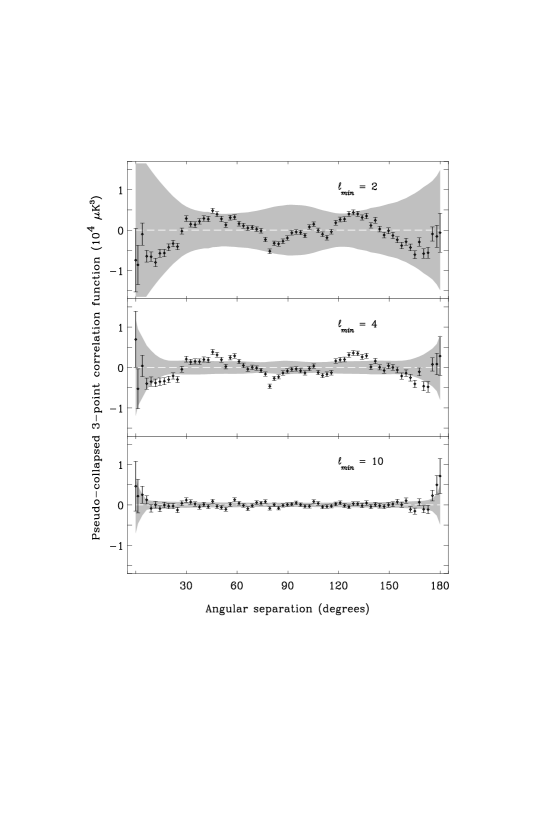
Figure 8.1: The ‘pseudo–collapsed’ three–point function as computed from the analysis of the two–year COBE–DMR data [from Hinshaw et al., 1995]. The quantity plotted is the analogue of our $\bigl{\langle}C_{3}(\alpha)\bigr{\rangle}T_{0}^{3}$ (see the text). Error bars represent instrument noise while the grey band represents the rms range of fluctuations due to a superposition of instrument noise and cosmic variance. Three different subtraction schemes are shown: the top, middle and bottom panels represent the cases $l_{min}=2,~{}4,~{}10$ respectively.

The idea is to confront our results for the mean $\bigl{\langle}C_{3}(\alpha)\bigr{\rangle}$ plus its cosmic variance ‘error bars’ with the experimental data as given in Figure 8.1. Roughly speaking, if the amplitude of our signal plus cosmic variance is larger than the actual data points plus the experimental noise given in the maps, then the analytic texture model considered in the present Chapter cannot be constrained by the experiment. If, on the other hand, our level of cosmic variance (on top of the collapsed three–point signal) lies below these points, then (based on the published analysis of the data) something might go wrong with the analytic model. Further study may then lead to modifications or even to the realisation that some of the assumptions is not fully met, thereby helping in the working out of a more realistic version of the model.

As we mentioned in the introduction, at the time of the writing up of this thesis, the work described here is still in progress. Preliminary (and conservative) estimates seem to indicate that the CMB mean three–point correlation function plus the cosmic variance predicted within the analytic texture model by Magueijo [1995] is consistent with the COBE–DMR two–year data reported in Figure 8.1. However, no definitive statement can be made, since careful checks in our computations are still to be performed.

A similar analysis based on a recently proposed analytic model for CMB anisotropy generation from cosmic strings [Perivolaropoulos, 1993; Gangui & Perivolaropoulos, 1995] is also under way [70], and we hope to report on this work in the near future.

The prospect is interesting in itself: it would give us a hint that, even on large angular scales, the analysis of non–Gaussian features in the structure of the cosmic microwave background radiation maps provides us with a tool to constrain models, or at least to make a consistency check of their predictions against experimental data.

Chapter 9 Global textures and the Doppler peaks

In the present Chapter we review recent work aimed at showing how global topological defects influence the shape of the angular power spectrum of the CMB radiation on small scales. As we explained before, the CMB fluctuations on large angular scales (greater than a few degrees) are caused by perturbations in the gravitational field via the Sachs–Wolfe effect. However, on intermediate scales, $0.1^{\circ}\mathrel{\raise 1.29167pt\hbox{$<$\kern-7.5pt\lower 4.30554pt\hbox{$\sim$}}}\theta\mathrel{\raise 1.29167pt\hbox{$<$\kern-7.5pt\lower 4.30554pt\hbox{$\sim$}}}2^{\circ}$, the main rôle is played by coherent oscillations in the baryon radiation plasma before the era of recombination. Unless the universe is reionised at some redshift $z>50$, these oscillations lead to the ‘Doppler peaks’ in the angular power spectrum. On even smaller scales the anisotropies are damped due to the finite thickness of the recombination shell [Bond & Efstathiou, 1984, 1987; Efstathiou, 1990], as well as by photon diffusion during recombination, due to the imperfect coupling between baryons and photons (Silk damping [Silk, 1968]).

Inflation–based cold dark matter models predict the location of the first peak to be at $\ell\sim 220/\sqrt{\Omega_{0}}$, with a height which is a few times the amplitude of the Sachs–Wolfe ‘plateau’ on large scales [Steinhardt, 1995]. Here we present a corresponding study for perturbations induced by global textures. As we will see below, the first Doppler peak is reduced to an amplitude comparable to that of the Sachs–Wolfe contribution, and it is shifted to $\ell\sim 350$. We also briefly comment on the relation between these results and what open models predict.

9.1 Acoustic oscillations and ${\Delta T\over T}$

The importance of the observations of anisotropies on angular scales ranging $0.1^{\circ}\mathrel{\raise 1.29167pt\hbox{$<$\kern-7.5pt\lower 4.30554pt\hbox{$\sim$}}}\theta\mathrel{\raise 1.29167pt\hbox{$<$\kern-7.5pt\lower 4.30554pt\hbox{$\sim$}}}2^{\circ}$, and smaller, cannot be over-emphasised. Presently a host of experiments scrutinise different regions of the sky trying to uncover the real amplitude and structure of the relic radiation. While the COBE–DMR data played undoubtedly an important rôle in determining the normalisation for the angular spectra predicted by the different models, it is clear now that the next important step towards discriminating between competing models lies on the degree scale. Whether it will be inflation [Steinhardt, 1993] or defect models [Kibble, 1980] the ‘final’ theory, able to explain faithfully the experimental data, is something that hopefully will not make us wait so long. The CMB anisotropies are a powerful tool to discriminate among these models by purely linear analysis. As we saw before, they are parameterised in terms of ${\cal C}_{\ell}$’s, defined (cf. Chapter 4) as the coefficients in the expansion of the angular correlation function

$$\langle C_{2}(\vartheta)\rangle={1\over 4\pi}\sum_{\ell}(2\ell+1){\cal C}_{\ell}P_{\ell}(\cos\vartheta).$$ (9.1)

For a scale invariant spectrum of perturbations $\ell(\ell+1){\cal C}_{\ell}$ is constant on large angular scales, say $\ell\stackrel{{\scriptstyle<}}{{\sim}}50$. Both inflation and topological defect models lead to approximately scale invariant spectra and therefore their shape on these scales does not help in our aim of finding a signature to distinguish between models.

On smaller scales the situation is more promising and we will see below how the predictions of global textures on the CMB angular spectrum profile depart from those expected in the standard CDM inflationary model. Disregarding Silk damping, gauge invariant linear perturbation analysis leads to [Durrer, 1994]

$${\delta T\over T}=\left[-{1\over 4}D_{g}^{(r)}+V_{j}\gamma^{j}-\Psi+\Phi\right]_{i}^{f}+\int_{i}^{f}(\Psi^{\prime}-\Phi^{\prime})d\tau~{},$$ (9.2)

where $\Phi$ and $\Psi$ are quantities describing the perturbations in the geometry (Bardeen potentials) and $\bf V$ denotes the peculiar velocity of the radiation fluid with respect to the overall Friedmann expansion. Primes stand for derivatives with respect to conformal time. $D_{g}^{(r)}$ specifies the intrinsic density fluctuation in the radiation fluid. There are several gauge invariant variables which describe density fluctuations; they all differ on super–horizon scales but coincide inside the horizon. Below we use another variable, $D_{r}$, for the radiation density fluctuation [Kodama & Sasaki, 1984]. Since the coherent oscillations giving rise to the Doppler peaks act only on sub–horizon scales, the choice of this variable is irrelevant for our calculation.

$\Phi$ , $\Psi$ and $D_{g}^{(r)}$ in Eq. (9.2) determine the anisotropies on large angular scales, and have been calculated for both inflation and defect models [Scott et al., 1995; Bennett & Rhie, 1993; Pen et al., 1994; Durrer & Zhou, 1995]. Generically, a scale invariant spectrum is predicted and thus the Sachs–Wolfe calculations yield mainly a normalisation for the different models. In this Chapter we present a computation for the Doppler contribution from global topological defects; in particular we perform our analysis for $\pi_{3}$–defects, textures [Turok, 1989], in a universe dominated by cold dark matter. Many of the features endowed by textures are also present in other global defects and we believe that the analysis we present below remains valid for these defects as well.

The Doppler contribution to the CMB anisotropies is given by

$$\left[{\delta T\over T}({\vec{x}},\hat{\gamma})\right]^{Doppler}={1\over 4}D_{r}({\vec{x}}_{rec},\eta_{rec})-{\vec{V}}({\vec{x}}_{rec},\eta_{rec})\cdot{\hat{\gamma}}~{},$$ (9.3)

where ${\vec{x}}_{rec}={\vec{x}}+{\hat{\gamma}}\eta_{0}$. In the previous formula ${\hat{\gamma}}$ denotes a direction in the sky and $\eta$ is the conformal time, with $\eta_{0}$ and $\eta_{rec}$ the present and recombination times, respectively.

9.2 Linear theory power spectra

To evaluate Eq. (9.3) we calculate $D_{r}$ and ${\vec{V}}$ at $\eta_{rec}$. We study a two–fluid system: baryons plus radiation, which prior to recombination are tightly coupled, and CDM.

We start off by considering the evolution equations in each fluid component as are given in the classic paper by Kodama & Sasaki [1984]. The evolution of the perturbation variables in a flat background, $\Omega=1$, can be expressed as

$$\begin{array}[]{lll}V^{\prime}_{r}+{a^{\prime}\over a}V_{r}&=&k\Psi+k{c_{s}^{2}\over 1+w}D_{r}\\ V^{\prime}_{c}+{a^{\prime}\over a}V_{c}&=&k\Psi\\ D^{\prime}_{r}-3w{a^{\prime}\over a}D_{r}&=&(1+w)[3{a^{\prime}\over a}\Psi-3\Phi^{\prime}-kV_{r}-{9\over 2}\left({a^{\prime}\over a}\right)^{2}k^{-1}(1+{w\rho_{r}\over\rho})V_{r}]\\ D^{\prime}_{c}&=&3{a^{\prime}\over a}\Psi-3\Phi^{\prime}-kV_{c}-{9\over 2}\left({a^{\prime}\over a}\right)^{2}k^{-1}(1+{w\rho_{r}\over\rho})V_{c}{}~{},\end{array}$$ (9.4)

where subscripts _r and _c denote the baryon–radiation plasma and CDM, respectively; $D,~{}V$ are density and velocity perturbations; $w=p_{r}/\rho_{r}$, $c_{s}^{2}=p^{\prime}_{r}/\rho^{\prime}_{r}$ and $\rho=\rho_{r}+\rho_{c}$.

Throughout this section we will normalise the scale factor as $a(\eta_{eq})=1$, where $\eta_{eq}$ stands for the conformal time at the time of equality between matter and radiation (we will come back to the usual convention $a(\eta_{0})=1$ at the end, when expressing our results). For a flat universe we have $(a^{\prime}/a)^{2}=8\pi Ga^{2}(\rho_{rad}+\rho_{mat})/3$, where both CDM and baryons are included in $\rho_{mat}$. Taking into account now the different scaling behaviour of both forms of energy with $a$, and defining $\tau\equiv(8\pi G/3)^{-1/2}(\rho_{eq}/2)^{-1/2}$, where $\rho_{eq}$ is the total energy density at equality, we get $a(\eta)+1=(\sqrt{2}+(\eta-\eta_{eq})/2\tau)^{2}$, which automatically satisfies $a_{eq}=1$, as it should. By further requiring that $a$ vanishes at the origin we get $\tau=\eta_{eq}/(2(\sqrt{2}-1))$ while the scale factor may be cast as

$$a(\eta)={\eta\over\tau}\left(1+{1\over 4}{\eta\over\tau}\right)~{}.$$ (9.5)

It is clear from this expression that for early (late) conformal times we recover the radiation (matter) dominated phase of expansion of the universe.

Furthermore, as both the energy density of baryons and CDM go as $\propto a^{-3}$ we have the ratio $\rho_{bar}/\rho_{cdm}\simeq$ const, and today yields $\Omega_{B}$. From this we may calculate $\rho_{bar}/\rho_{rad}=(\rho_{bar}/\rho_{cdm})(\rho_{cdm}/\rho_{rad})\simeq\Omega_{B}a$. Applying this to $w$ and $c_{s}^{2}$ of Eq. (9.4) we get their time dependences as follows

$$w\simeq{1\over 3}(1+\Omega_{B}a)^{-1}~{}~{}~{};~{}~{}~{}c_{s}^{2}\simeq{1\over 3}(1+{\textstyle{3\over 4}}\Omega_{B}a)^{-1}~{}.$$ (9.6)

The only place where the ‘seeds’ (texture–seeds or whatever) enter the system (9.4) is through the potentials $\Psi$ and $\Phi$. These potentials may be split into a part coming from standard matter and radiation, and a part due to the seeds, e.g., $\Psi=\Psi_{(c,r)}+\Psi_{seed}$ where $\Psi_{seed},\Phi_{seed}$ are determined by the energy momentum tensor of the seed; the global texture in our case. Having said this, one may easily see how the seed source terms arise [Durrer, 1994].

It is our aim now to get rid of the velocity perturbations and express the system (9.4) as two second order equations for $D_{r}$ and $D_{c}$. For the sake of simplicity in these intermediate steps let us neglect, for the time being, the source terms (we will incorporate them at the end). After straightforward algebra we find

$$V_{c}={12\pi Ga^{2}\rho_{r}(1+w)V_{r}-kD^{\prime}_{c}\over 12\pi Ga^{2}\rho_{r}(1+w)+k^{2}}$$ (9.7)

and

$$V_{r}=-{\left(\rho_{c}D^{\prime}_{c}+\rho_{r}D^{\prime}_{r}-3{a^{\prime}\over a}w\rho_{r}D_{r}+k^{2}(12\pi Ga^{2})^{-1}(1+w)^{-1}(D^{\prime}_{r}-3{a^{\prime}\over a}wD_{r})\right)\over k\left(k^{2}(12\pi Ga^{2})^{-1}+\rho_{r}(1+w)+\rho_{c}\right)}~{},$$ (9.8)

which express the velocity perturbations in both fluids in terms of the intrinsic density perturbations and the background variables. After long (and tedious) computations in which we differentiate $V_{r}$ and $V_{c}$ from Eqs. (9.7), (9.8) and we substitute back into Eqs. (9.4), including this time the seed source term, we finally derive two second order equations for $D_{r}$ and $D_{c}$, namely

$$D_{r}^{\prime\prime}+{a^{\prime}\over a}[1+3c_{s}^{2}-6w+F^{-1}\rho_{c}]D_{r}^{\prime}-{a^{\prime}\over a}\rho_{c}F^{-1}(1+w)D_{c}^{\prime}$$

$$+4\pi Ga^{2}[\rho_{r}(3w^{2}-8w+6c_{s}^{2}-1)-2F^{-1}w\rho_{c}(\rho_{r}+\rho_{c})$$

$$+\rho_{c}(9c_{s}^{2}-7w)+{k^{2}\over 4\pi Ga^{2}}c_{s}^{2}]D_{r}-4\pi Ga^{2}\rho_{c}(1+w)D_{c} = (1+w)S~{};\hskip 28.45274pt$$ (9.9)

$$D_{c}^{\prime\prime}+{a^{\prime}\over a}[1+(1+w)F^{-1}\rho_{r}(1+3c_{s}^{2})]D_{c}^{\prime}-{a^{\prime}\over a}(1+3c_{s}^{2})F^{-1}\rho_{r}D_{r}^{\prime}$$

$$-4\pi Ga^{2}\rho_{c}D_{c}-4\pi Ga^{2}\rho_{r}(1+3c_{s}^{2})[1-2(\rho_{r}+\rho_{c})F^{-1}w]D_{r} = S~{},$$ (9.10)

where $F\equiv k^{2}(12\pi Ga^{2})^{-1}+\rho_{r}(1+w)+\rho_{c}$ and $S$ denotes a source term, which in general is given by $S=4\pi Ga^{2}(\rho+3p)^{seed}$. In our case, where the seed is described by a global scalar field $\phi$, we have $S=8\pi Ga^{2}(\dot{\phi})^{2}$.

From numerical simulations one finds that the integral of $a^{2}|\dot{\phi}|^{2}$ over a shell of radius $k$ can be modeled by [Durrer & Zhou, 1995]

$$a^{2}\langle|\dot{\phi}|^{2}\rangle(k,\eta)\ =\ {{1\over 2}A\tilde{\eta}^{2}\over\sqrt{\eta}[1+\alpha(k\eta)+\beta(k\eta)^{2}]}~{},$$ (9.11)

with $\tilde{\eta}$ denoting the symmetry breaking scale of the phase transition leading to texture formation (cf. §2.2). The parameters in (9.11) are $A\sim 3.3$, $\alpha\sim-0.7/(2\pi)$ and $\beta\sim 0.7/(2\pi)^{2}$. On super–horizon scales, where the source term is important, this fit is accurate to about $10\%$. Analytical estimates support this finding [54]. On small scales the accuracy reduces to a factor of 2. By using this fit in the calculation of $D_{r}$ and $D_{c}$ from Eqs. (9.9), (9.10) we effectively neglect the time evolution of phases of $(\phi^{\prime})^{2}$; the incoherent evolution of these phases may smear out subsequent Doppler peaks [Albrecht et al., 1995], but will not affect substantially the height of the first peak.

9.3 Choosing initial conditions

In defect models of large–scale structure formation one usually assumes that the universe begins in a hot, homogeneous state. All perturbation variables are zero, and the primordial fields (e.g., the global field $\phi$ in our case) are in thermal equilibrium in the unbroken symmetry phase. When the phase transition occurs the field $\phi$ leaves thermal equilibrium and enters the process of phase ordering. The large scales of interest to us get perturbed when crossing the horizon, long after the phase transition took place.

Before the phase transition the defect fields have no long–range correlations. The dynamics of the transition as well as the field ordering are completely causal processes. Isotropy and the vanishing correlation function of the defect’s stress–energy tensor on super–horizon scales lead to the power spectrum of the source term to take the form of white noise for $k\eta<<1$.

Following the phase transition, the distribution of the defect field enters a ‘scaling’ regime rapidly [Pen et al., 1994], and so numerical simulations need to be performed only within a reduced dynamical range: from ‘natural’ initial conditions (namely, no correlations on super–horizon scales) and for a few expansion times. This is enough to produce a realistic field distribution on large scales.

Going back now to our set of Eqs. (9.9), (9.10) we will specify our initial conditions as follows: for a given scale $k$ we choose the initial time $\eta_{in}$ such that the perturbation is super–horizon–sized and the universe is radiation dominated. In this limit the evolution equations reduce to

$$D_{r}^{\prime\prime}-{2\over\eta^{2}}D_{r} = {4\over 3}{A\epsilon\over\sqrt{\eta}}{}~{};$$ (9.12)

$$D_{c}^{\prime\prime}+{3\over\eta}D_{c}^{\prime}-{3\over 2\eta}D_{r}^{\prime}-{3\over 2\eta^{2}}D_{r} = {A\epsilon\over\sqrt{\eta}}~{},$$ (9.13)

with particular solutions

$$D_{r}\ =\ -{16\over 15}\epsilon A\eta^{3/2}\ ;\ D_{c}\ =\ -{4\over 7}\epsilon A\eta^{3/2}\ .$$ (9.14)

In the above equations we have introduced $\epsilon\equiv 4\pi G\tilde{\eta}^{2}$, the only free parameter in the model. We consider perturbations seeded by the texture field, and therefore it is incorrect to add a homogeneous growing mode to the above solutions. With these initial conditions, Eqs. (9.9), (9.10) are easily integrated numerically, leading to the spectra for $D_{r}(k,\eta_{rec})$ and $D_{r}^{\prime}(k,\eta_{rec})$ (see Figure 9.1).

Figure 9.1: The dimensionless power spectra, $k^{3}|D_{r}|^{2}$ (solid line) and $k|D^{\prime}_{r}|^{2}$ (dashed line) in units of $(A\epsilon)^{2}$, are shown as functions of $k$. These are exactly the quantities which enter in the expression for the ${\cal C}_{\ell}$’s. We set $h=0.5~{},~{}\Omega_{B}=0.05$ and $z_{rec}=1100$.

9.4 Angular power spectrum from global textures

In this section we calculate the expression for ${\cal C}_{\ell}$ as function of the baryon–radiation power spectrum and its derivative, evaluated at $\eta_{rec}$.

Following a standard procedure [Durrer, 1994] we express the Fourier transform of the velocity perturbation in the radiation fluid as

$${\vec{V}}({\vec{k}})\simeq-{i{\vec{k}}D_{r}^{\prime}({\vec{k}})\over k^{2}(1+w)}~{}.$$ (9.15)

Now, let us Fourier transform the Doppler contribution to the anisotropies as given by Eq. (9.3). Using (9.15) we get

$$\left[{\delta T\over T}({\vec{k}},\eta_{0},\mu)\right]^{Doppler}=e^{ik\eta_{0}\mu}\left({1\over 4}D_{r}({\vec{k}},\eta_{rec})+{i\mu D_{r}^{\prime}({\vec{k}},\eta_{rec})\over k(1+w)}\right)$$ (9.16)

where $\mu={\hat{k}}\cdot\hat{\gamma}$. Now, it will prove useful to perform an expansion in Legendre polynomials as follows

$$\left[{\delta T\over T}({\vec{k}},\eta_{0},\mu)\right]^{Doppler}=\sum_{\ell=0}^{\infty}i^{\ell}\Delta_{\ell}({\vec{k}},\eta_{0})P_{\ell}(\mu)~{}.$$ (9.17)

After some algebra we get the coefficients $\Delta_{\ell}$ in the previous expansion given by

$${\Delta_{\ell}({\vec{k}},\eta_{0})\over(2\ell+1)}={1\over 4}D_{r}({\vec{k}},\eta_{rec})j_{\ell}(k\eta_{0})+{D_{r}^{\prime}({\vec{k}},\eta_{rec})\over k(1+w)}j^{\prime}_{\ell}(k\eta_{0})~{},$$ (9.18)

where $j_{\ell}$ denotes the spherical Bessel function of order $\ell$ and $j^{\prime}_{\ell}$ stands for its derivative with respect to the argument. Now we claim that we may cast the Doppler contribution to the multipole coefficients ${\cal C}_{\ell}$ as follows

$${\cal C}_{\ell}^{(Doppler)}={2\over\pi}\int dk~{}k^{2}{|\Delta_{\ell}({\vec{k}},\eta_{0})|^{2}\over(2\ell+1)^{2}}~{}.$$ (9.19)

To prove this we make use of the ergodic hypothesis and substitute the ensemble average by an integral over all possible observers. Thus we may write the left–hand side of Eq. (9.1) as follows

$$\bigl{\langle}{\Delta T\over T}({\vec{x}},\hat{\gamma}){\Delta T\over T}^{*}({\vec{x}},\hat{\gamma}^{\prime})\bigr{\rangle}=\int d^{3}x\int{d\Omega_{\hat{\gamma}}d\Omega_{\hat{\gamma}^{\prime}}\over 8\pi^{2}}{\Delta T\over T}({\vec{x}},\hat{\gamma}){\Delta T\over T}^{*}({\vec{x}},\hat{\gamma}^{\prime})~{},$$ (9.20)

with the constraint $\hat{\gamma}\cdot\hat{\gamma}^{\prime}=\cos\vartheta$, and where ^∗ denotes complex conjugation. Upon using Parseval’s relation to transform the $\int d^{3}x$ integral into an integral on ${\vec{k}}$ we see that Eq. (9.20) can be cast as

$${1\over(2\pi)^{3}}\int d^{3}k\sum_{\ell,\ell^{\prime}}i^{\ell-\ell^{\prime}}\Delta_{\ell}({\vec{k}},\eta_{0})\Delta_{\ell^{\prime}}^{*}({\vec{k}},\eta_{0})\int{d\Omega_{\hat{\gamma}}d\Omega_{\hat{\gamma}^{\prime}}\over 8\pi^{2}}P_{\ell}(\mu)P_{\ell^{\prime}}(\mu^{\prime})~{}.$$ (9.21)

Now, the last integral in Eq. (9.21) may be written as

$$\int{d\Omega_{\hat{\gamma}}d\Omega_{\hat{\gamma}^{\prime}}\over 8\pi^{2}}\delta(\hat{\gamma}\cdot\hat{\gamma}^{\prime}-\cos\vartheta)P_{\ell}({\hat{k}}\cdot\hat{\gamma})P_{\ell^{\prime}}({\hat{k}}\cdot\hat{\gamma}^{\prime}),$$ (9.22)

where we introduced a Dirac delta to enforce the constraint on the $\hat{\gamma}$’s. Standard algebra like the one used in Chapter 4 yields Eq. (9.20) in the form

$$\bigl{\langle}C_{2}(\vartheta)\bigr{\rangle}={1\over(2\pi)^{3}}\int d^{3}k\sum_{\ell=0}^{\infty}{|\Delta_{\ell}({\vec{k}},\eta_{0})|^{2}\over(2\ell+1)}P_{\ell}(\cos\vartheta)~{}.$$ (9.23)

If we assume now that $|\Delta_{\ell}({\vec{k}},\eta_{0})|^{2}$ depends only on the absolute value $k$, we can integrate out the directions ${\hat{k}}$ and, upon comparison with the expansion (9.1) it is easy to see that the claimed result is achieved. Finally, knowing the spectra for $D_{r}$ and $D_{r}^{\prime}$ we calculate the Doppler contribution to the ${\cal C}_{\ell}$’s according to

$${\cal C}_{\ell}={2\over\pi}\int dk\left[{k^{2}\over 16}|D_{r}(k,\eta_{rec})|^{2}j_{\ell}^{2}(k\eta_{0})+(1+w)^{-2}|D_{r}^{\prime}(k,\eta_{rec})|^{2}(j_{\ell}^{\prime}(k\eta_{0}))^{2}\right]~{},$$ (9.24)

where we drop the label ^(Doppler) from now on. As we mentioned above, the source term of equations (9.9) and (9.10) was estimated from numerical simulations of the evolution of the global scalar field $\phi$. These simulations give a fit for the absolute value of $\phi$ and therefore we can say nothing with regard to phases. This also implies that we cannot evaluate the crossed term missing in Eq. (9.24), which we neglect as a first approximation to the problem. Integrating Eq. (9.24), we obtain the Doppler contribution to the angular spectrum of the CMB anisotropies [Durrer, Gangui & Sakellariadou, 1995]. We plot the result in Figure 9.2.

Figure 9.2: The angular power spectrum for the Doppler contribution to the CMB anisotropies is shown in units of $\epsilon^{2}$. We set cosmological parameters $h=0.5~{},~{}\Omega_{B}=0.05$ and $z_{rec}=1100$.

9.5 Discussion

As we see from the plot, the angular power spectrum $\ell(\ell+1){\cal C}_{\ell}$ yields the Doppler peaks. For $\ell<1000$, we find three peaks located at $\ell=365$, $\ell=720$ and $\ell=950$. Silk damping, which we have not taken into account here, will decrease the relative amplitude of the third peak with respect to the second one; however it will not affect substantially the height of the first peak. Our most important results regard the amplitude and position of the first Doppler peak, for which we find

$$\ell(\ell+1){\cal C}_{\ell}\left|{}_{{~{}}_{\!\!\ell\sim 360}}=5\epsilon^{2}~{}.\right.$$ (9.25)

It is interesting to notice that the position of the first peak is displaced by $\Delta\ell\sim 150$ towards smaller angular scales than in standard inflationary models [Steinhardt, 1995]. This might be due to the difference in the growth of super–horizon perturbations, which is $D_{r}\propto\eta^{3/2}$ in our case (cf. Eqs. (9.14)), and $D_{r}\propto\eta^{2}$ for inflationary models.

One may understand the height of the first peak from the following analytic estimate: matching the sub–horizon with the super–horizon solutions of Eq. (9.10), in the matter dominated era, one finds $D_{c}\sim-{2\over 5}A\epsilon(k/2\pi)^{1/2}\eta^{2}$. From Eq. (9.9) we then obtain in this limit $D_{r}\approx A\epsilon k^{-3/2}$. Plugging this latter value into Eq. (9.24) we get roughly $\ell(\ell+1){\cal C}_{\ell}\sim(A\epsilon)^{2}$, for the height of the first peak.

Let us now compare our value for the Doppler peak with the level of the Sachs–Wolfe plateau [Bennett & Rhie, 1993; Pen et al., 1994; Durrer & Zhou, 1995]

$$\ell(\ell+1){\cal C}_{\ell}\left|{}_{{~{}}_{\!\!SW}}\sim(6-14)\epsilon^{2}.\right.$$ (9.26)

It is apparent from Eqs. (9.25) and (9.26) that the Doppler contribution from textures is substantially smaller than for inflationary models.

Normalising with the COBE–DMR experiment [Smoot et al., 1992; Górski et al., 1994]

$$\ell(\ell+1){\cal C}_{\ell}\left|{}_{{~{}}_{\!\!COBE}}\sim 8\times 10^{-10}\right.~{},$$

one finds the symmetry breaking energy scale when textures are produced in the early universe, and from this $\epsilon\sim 10^{-5}$. This value for $\epsilon$ depends of course upon the numerical simulations, Refs. [22, 161, 54].

We believe that this result, stating that the first Doppler peak has a height comparable to the Sachs–Wolfe plateau, is valid for all global defects. This depends crucially on the $1/\sqrt{\eta}$ behavior of $(a\dot{\phi})^{2}={\phi^{\prime}}^{2}$ on large scales (cf. Eq. (9.11)), which is a generic feature of global defects: on super–horizon scales $\dot{\phi}^{2}(k)$ represents white noise superimposed on the average given by $\bigl{\langle}{\phi^{\prime}}^{2}\bigr{\rangle}\sim{\phi^{\prime}}^{2}(k=0)\propto 1/\eta^{2}$ (the usual scaling behaviour). The Fourier transform of ${\phi^{\prime}}^{2}$ determines the fluctuations on this background on a given comoving scale $\lambda$. A patch of size $\lambda$ consists of $N=(\lambda/\eta)^{3}$ independent horizon–sized volumes. The fluctuation ${\phi^{\prime}}^{2}(k)$ on this scale is thus proportional to $\bigl{\langle}{\phi^{\prime}}^{2}\bigr{\rangle}/\sqrt{N}\propto 1/\sqrt{\eta}$. Notice that this argument does not apply for local cosmic strings.

The displacement of the peaks towards smaller scales is reminiscent of open models [e.g., Kamionkowski, Spergel & Sugiyama, 1994], where the first Doppler peak is located approximately at $\ell_{peak}\simeq 220/\sqrt{\Omega_{0}}$. A value $\Omega_{0}\simeq 0.3$ would produce $\ell_{peak}\simeq 365$ for the first peak, as we actually find. However, the amplitude of the peaks within open inflationary models is still much larger than what we find from global defects.

Similar results to those worked out in the present Chapter were independently derived in [Crittenden & Turok, 1995]. Following a different approach, these authors calculate the Doppler peaks from cosmic textures in the synchronous gauge. A main assumption of that analysis is that spatial gradients in the scalar field are frozen outside the horizon, and therefore time derivatives are negligible. This is not the case in the simulations for the texture source term from Durrer & Zhou [1995]. Apart from this we basically agree with the shape and position of their Doppler peaks. Regarding the height of the peaks, however, these authors seem to obtain an amplitude similar to that predicted in standard inflation–based models, unlike what we find.

Based on our analysis we conclude that if the existence of Doppler peaks is indeed confirmed (recall that not all the teams agree in their findings on the $\theta\sim 1^{\circ}$ scale) and the height of the first peak is larger than about twice the level of the Sachs–Wolfe plateau, namely

$$\ell(\ell+1){\cal C}_{\ell}\left|{}_{{~{}}_{\!\!peak}}>2\times 10^{-9}\right.~{},$$

and if the first peak is positioned at $\ell<300$, then global topological defects are ruled out. On the other hand, if the first Doppler peak is positioned at $\ell\sim 350$ and its height is below the above value, global defects are strongly favored if compared to standard cold dark matter inflationary models. This is a clear fingerprint, within present observational capabilities, to distinguish among these two competing models of structure formation.

Bibliography

- [1] Abbott, L.F., Fahri, E. & Wise, M.B. [1982], Phys. Lett. B117, 29.
- [2] Abbott, L.F. & Wise, M.B. [1984], Ap. J. Lett. 282, L47.
- [3] Abbott, L.F. & Wise, M.B. [1984b], Nucl. Phys. B244, 541.
- [4] Adams, F.C., Bond, J.R., Freese, K., Frieman, J. & Olinto, A. [1993], Phys. Rev. D47, 426.
- [5] Adams, F.C., Freese, K. & Guth, A.H. [1991], Phys. Rev. D43, 965.
- [6] Albrecht, A., Coulson, D., Ferreira, P. & Magueijo, J. [1995], Imperial Preprint /TP/94–95/30.
- [7] Albrecht, A. & Steinhardt, P. [1982], Phys. Rev. Lett. 48, 1220.
- [8] Albrecht, A., Steinhardt, P.J., Turner, M.S. & Wilczek, F. [1982], Phys. Rev. Lett. 48, 1437.
- [9] Allen, T.J., Grinstein, B. & Wise, M.B. [1987], Phys. Lett. B197, 66.
- [10] Allen, B. & Shellard, E.P.S. [1990], Phys. Rev. Lett. 64, 119.
- [11] Amendola, L., Baccigalupi, C. & Occhionero, F. [1995], astro–ph/9504097 preprint.
- [12] Bardeen, J.M., Steinhardt, P.J. & Turner, M.S. [1983], Phys. Rev. D28, 679,1983..
- [13] Barrow, J.D. [1990], Phys. Lett. B235, 40.
- [14] Barrow, J.D. & Coles, P. [1990], M. N. R. A. S. 244, 188.
- [15] Barrow, J.D. & Liddle, A.R. [1993], Phys. Rev. D47, R5213.
- [16] Barrow, J.D. & Maeda, K. [1990], Nucl. Phys. B341, 294.
- [17] Barrow, J.D. & Saich, P. [1990], Phys. Lett. B249, 406.
- [18] Bennett, C.L., et al. [1992], Ap. J. Lett. 396, L7.
- [19] Bennett, C.L., et al. [1994], Ap. J. 430, 423.
- [20] Bennett, D.P. & Bouchet, F.R. [1988], Phys. Rev. Lett. 60, 257.
- [21] Bennett, D.P. & Rhie, S.H. [1990], Phys. Rev. Lett. 65, 1709.
- [22] Bennett, D.P. & Rhie, S.H. [1993], Ap. J. Lett. 406, L7.
- [23] Bennett, D.P., Rhie, S.H. & Weinberg, D.H. [1993], preprint.
- [24] Bennett, D.P., Stebbins, A. & Bouchet, F.R. [1992], Ap. J. Lett. 399, L5.
- [25] Bond, J.R. [1988], in The Early Universe, Unruh, W. & Semenoff, G., eds. (Reidel, Dordrecht).
- [26] Bond, J.R. & Efstathiou, G. [1984], Ap. J. Lett. 285, L45.
- [27] Bond, J.R. & Efstathiou, G. [1987], M. N. R. A. S. 226, 655.
- [28] Borrill, J., et al. [1994], Phys. Rev. D50, 2469.
- [29] Bouchet, F. R., Bennett, D. P. & Stebbins, A. [1988], Nature 335, 410.
- [30] Bowick, M., Chandar, L., Schiff, E. & Srivastava, A. [1994], Science 236, 943.
- [31] Boyanovski, D., et al. [1995], Preprint PITT–09–95; Phys. Rev. D51, 4419.
- [32] Brandenberger, R. [1993], Topological Defects and Structure Formation, EPFL lectures, Lausanne, Switzerland.
- [33] Brandenberger, R. [1995], Modern Cosmology and Structure Formation, TASI–94 Lectures at Boulder, Donoghue, J., ed. (World Scientific, Singapore).
- [34] Brandenberger, R. & Kahn, R. [1984], Phys. Rev. D29, 2172.
- [35] Brandenberger, R., Kaiser, N., Shellard, E.P.S. & Turok, N. [1987], Phys. Rev. D36, 335.
- [36] Bunch, T. & Davies, P. [1978], Proc. R. Soc. Lon. A360, 117.
- [37] Bunn, E.,Hoffman, Y. & Silk, J. [1994], Ap. J. 425, 359.
- [38] Callan, C. & Coleman, S. [1977], Phys. Rev. D16, 1762.
- [39] Cardoso, G.L. & Ovrut, B.A. [1993], CERN Preprint.
- [40] Carr, B.J. & Rees, M.J. [1984], M. N. R. A. S. 206, 801.
- [41] Carrol, S.M., Press, W.H. & Turner, E.L. [1992], Ann. Rev. Astron. and Astrophys. 30, 499.
- [42] Castagnino, M.A., Gangui, A., Mazzitelli, F.D. & Tkachev, I.I. [1993], Class. Quant. Grav. 10, 2495.
- [43] Chuang, I., Durrer, R., Turok, N. & Yurke, B. [1991], Science 251, 1336.
- [44] Coles, P. & Lucchin, F. [1995], Cosmology: The origin and evolution of cosmic structure (Wiley, New York).
- [45] Copeland, E. [1993], in The physical universe: The interface between cosmology, astrophysics and particle physics, eds. Barrow, J.D., et al. (Sringer–Verlag).
- [46] Coulson, D., Ferreira, P., Graham, P. & Turok, N. [1994], Nature 368, 27.
- [47] Crittenden, R.G. & Turok, N. [1995], Princeton University Preprint, PUPT–94–1545.
- [48] de Gennes, P. [1974], The Physics of Liquid Crystals (Clarendon Press, Oxford).
- [49] Dodelson, S. & Jubas, J.M. [1995], Ap. J. 439, 503.
- [50] Dolan, L. & Jackiw, R. [1974], Phys. Rev. D9, 3320.
- [51] Dolgov, A. & Freese, K. [1995], submitted to Phys. Rev. D, hep–ph/9408214.
- [52] Durrer, R. [1994], Fund. of Cosmic Physics 15, 209.
- [53] Durrer, R., Gangui, A. & Sakellariadou, M. [1995], SISSA–83/95/A, astro–ph/9507035.
- [54] Durrer, R. & Zhou, Z.H. [1995], Zürich University Preprint, ZH–TH19/95, astro–ph/9508016.
- [55] Durrer, R., Howard, A. & Zhou, Z.H. [1994], Phys. Rev. D49, 681.
- [56] Edmonds, A. R. [1960], Angular Momentum in Quantum Mechanics (Princeton University Press).
- [57] Efstathiou, G. [1990], in Physics of the early Universe Peacock, J.A., et al., eds. (New York: Adam Hilger).
- [58] Ellis, G.F.R. [1991], in Proc. Banff Summer Research Institute on Gravitation, Mann, R. & Wesson, P., eds. (Singapore: World Scientific).
- [59] Ellis, G.F.R. & Rothman, T. [1993], Lost Horizons, preprint.
- [60] Fabbri, R., Lucchin, F. & Matarrese, S. [1987], Ap. J. 315, 1.
- [61] Falk, T., Rangarajan, R. & Srednicki, M. [1993], Ap. J. Lett. 403, L1.
- [62] Freese, K., Frieman, J.A. & Olinto, A.V. [1990], Phys. Rev. Lett. 65, 3233.
- [63] Freese, K. [1994], in Yamada Conference XXXVII: Evolution of the Universe and its Observational Quest, Tokyo, Japan 1993, preprint astro–ph/9310012.
- [64] Fry, J.N. [1984], Ap. J. 279, 499.
- [65] Ganga, K., Cheng, E., Meyer, S., Page, L. [1993], Ap. J. Lett. 410, L57.
- [66] Gangui, A. [1994], Phys. Rev. D50, 3684.
- [67] Gangui, A. [1995], in Birth of The Universe & Fundamental Physics, Occhionero, F., ed. (Heidelberg: Springer–Verlag). in press.
- [68] Gangui, A., Lucchin, F., Matarrese, S. & Mollerach, S. [1994], Ap. J. 430, 447.
- [69] Gangui, A., Mazzitelli, F.D. & Castagnino, M.A. [1991], Phys. Rev. D43, 1853.
- [70] Gangui, A. & Mollerach, S. [1995], work in progress.
- [71] Gangui, A. & Perivolaropoulos, L. [1995], Ap. J. 447, 1.
- [72] Gibbons, G. & Hawking, S. [1977], Phys. Rev. D15, 2738.
- [73] Gliner, E.B. [1965], Zh. Eksp. Teor. Fiz. 49, 542. [Sov. Phys. JETP 22, 378 (1965)].
- [74] Gliner, E.B. [1970], Dokl. Akad. Nauk SSSR 192, 771. [Sov. Phys. Dokl. 15, 559 (1970)].
- [75] Goldwirth, D.S. & Piran, T. [1992], Phys. Rep. 214, 223.
- [76] Goncharov, A.S., Linde, A.D. & Mukhanov, V.F. [1987], Int. J. Mod. Phys. A2, 561.
- [77] Górski, K.M., Hinshaw, G., Banday, A.J., Bennett, C.L., Wright, E.L., Kogut, A., Smoot, G.F. & Lubin, P. [1994], Ap. J. Lett. 430, L89.
- [78] Gott, J.R., Park, C., Juszkiewicz, R., Bies, W.E., Bennett, D., Bouchet, F.R. & Stebbins, A. [1990], Ap. J. 352, 1.
- [79] Gott, R. [1985], Ap. J., 288, 422.
- [80] Graham, P., Turok, N., Lubin, P.M. & Schuster, J.A. [1993], PUP–TH–1408 preprint.
- [81] Guth, A.H. [1981], Phys. Rev. D23, 347.
- [82] Guth, A.H. & Pi, S.–Y. [1985], Phys. Rev. D32, 1899.
- [83] Guth, A.H. & Tye, S.–H. [1980], Phys. Rev. Lett. 44, 631.
- [84] Guth, A.H. & Weinberg, E. [1983], Nucl. Phys. B212, 321.
- [85] Halliwell, J.J. [1989], Phys. Rev. D39, 2912.
- [86] Hancock, S., Davies, R.D., Lasenby, A.N., Gutierrez de la Cruz, C.M., Watson, R.A., Rebolo, R. & Beckman, J.E. [1994], Nature 367, 333.
- [87] Hara T. & Miyoshi S. [1993], Ap. J. 405, 419.
- [88] Harrison, R. [1970], Phys. Rev. D1, 2726.
- [89] Hendry, P.C., Lawson, N.S., Lee, R.A.M., McClintock, P.V.E. & Williams, C.D.H. [1994], Nature 368, 315.
- [90] Hilton, P.J. [1953], Introduction to homotopy theory (Cambridge: Cambridge University Press).
- [91] Hindmarsh M. [1994], Ap. J. 431, 534.
- [92] Hindmarsh, M. & Kibble, T. [1994], Rep. Prog. Phys., in press (preprint hep–ph/9411342).
- [93] Hinshaw, G., Kogut, A., Górski, K.M., Banday, A.J., Bennett, C.L., Lineweaver, C., Lubin, P., Smoot, G.F. & Wright, E.L. [1994], Ap. J. 431, 1.
- [94] Hinshaw, G., Banday, A.J., Bennett, C.L., Górski, K.M. & Kogut, A. [1995], Ap. J. Lett. 446, L67.
- [95] Hodges, H.M., Blumenthal, G.R., Kofman, L.A. & Primack, J.R. [1990], Nucl. Phys. B335, 197.
- [96] Hu, W., Scott, D. & Silk, J. [1994], Phys. Rev. D49, 648.
- [97] Hu, W., Sugiyama, N. & Silk, J. [1995], Nature, in press.
- [98] Jones, B. & Wyse, R. [1985], Astron. Astrophys. 149, 144.
- [99] Kaiser, N. & Stebbins, A. [1984], Nature 310, 391.
- [100] Kamionkowski, M., Spergel, D.N. & Sugiyama, N. [1994], Ap. J. Lett. 426, L57.
- [101] Kibble, T.W.B. [1976], J. Phys. A9, 1387.
- [102] Kibble, T.W.B. [1980], Phys. Rep. 67, 183.
- [103] Kibble, T.W.B., Lazarides, G. & Shafi, Q. [1982], Phys. Lett. B113, 237.
- [104] Kirzhnits, D.A. & Linde, A.D. [1974], Sov. Phys. JETP 40, 628.
- [105] Kirzhnits, D.A. & Linde, A.D. [1976], Ann. Phys. 101, 195.
- [106] Kodama, H. & Sasaki, M. [1984], Prog. Theor. Phys. Suppl. 78, 1.
- [107] Kofman, L.K., Blumenthal, G.R., Hodges, H. & Primack, J.R. [1990], in Large–Scale Structures and Peculiar Motions in the Universe, Latham, D.W. & da Costa, L.N. eds., ASP Conference Series, Vol. 15.
- [108] Kofman, L.A., Linde, A.D. & Starobinskii, A.A. [1985], Phys. Lett. B157, 361.
- [109] Kofman, L.A., Linde, A.D. & Starobinskii, A.A. [1994], Phys. Rev. Lett. 24, 3195.
- [110] Kogut, A., Banday, A.J., Bennett, C.L., Hinshaw, G., Lubin, P. & Smoot, G.F. 1994, Ap. J. Lett. 439, L29.
- [111] Kolb, E.W. [1994], in 42nd Scottish Universities Summer School in Physics, St. Andrews, Scotland, August 1993. in press.
- [112] Kolb, E.W. & Turner, M.S. [1990] The Early Universe (New York: Addison–Wesley).
- [113] Kolb, E.W. & Vadas, S.L. [1994], Phys. Rev. D50, 2479.
- [114] La, D. & Steinhardt, P.J. [1989], Phys. Rev. Lett. 62, 376.
- [115] Langacker, P. & Pi, S.–Y. [1980], Phys. Rev. Lett. 45, 1.
- [116] Langer, S. [1992], in Solids far from equilibrium, Godrèche, C., ed. (Cambridge: Cambridge University Press).
- [117] Liddle, A.R. & Lyth, D.H. [1992], Phys. Lett. B291, 391.
- [118] Liddle, A.R. & Lyth, D.H. [1993], Phys. Rep. 231, 1.
- [119] Liddle, A.R. & Turner, M.S. [1994], Phys. Rev. 50, 758.
- [120] Linde, A.D. [1974], Pis’ma Zh. Eksp. Teor. Fiz. 19, 320. [JETP Lett. 19, 183 (1974)].
- [121] Linde, A.D. [1979], Rep. Progr. Phys. 42, 389.
- [122] Linde, A.D. [1982a], Phys. Lett. B108, 389.
- [123] Linde, A.D. [1982b], Phys. Lett. B116, 335.
- [124] Linde, A.D. [1983a], Phys. Lett. B129, 177.
- [125] Linde, A.D. [1983b], Nucl. Phys. B216, 421.
- [126] Linde, A.D. [1985], Phys. Lett. B162, 281.
- [127] Linde, A.D. [1990], Particle Physics and Inflationary Cosmology (Harwood, Chur, Switzerland).
- [128] Linde, A.D. [1994], Phys. Rev. D49, 748.
- [129] Lindley, D. [1985], unpublished.
- [130] Luo, X. [1994], Ap. J. Lett. 427, L71.
- [131] Luo, X. & Schramm, D.N. [1993], Phys. Rev. Lett. 71, 1124.
- [132] Lucchin, F. & Matarrese, S. [1985], Phys. Rev. D32, 1316.
- [133] Lucchin, F., Matarrese, S. & Mollerach, S. [1992], Ap. J. Lett. 401, L49.
- [134] Lyth, D.H. [1985], Phys. Rev. D31, 1792.
- [135] Lyth, D.H. & Stewart, E.D. [1992], Phys. Lett. B274, 168.
- [136] Madsen, M.S. & Ellis, G.F.R. [1988], M.N.R.A.S. 234, 67.
- [137] Magueijo, J. [1992], Phys. Rev. D46, 1368.
- [138] Magueijo, J. [1995], Phys. Rev. D52, 689.
- [139] Malaney, R.A. & Mathews, G.J. [1993], Phys. Rep. 229, 145.
- [140] Martínez–González, E., Sanz, J.L. & Silk, J. [1992], Phys. Rev. D46, 4193.
- [141] Matarrese, S., Ortolan, A. & Lucchin, F. [1989], Phys. Rev. D40, 290.
- [142] Mather, J. C., et al. [1994], Ap. J. 420, 439.
- [143] Mermin, M. [1979] , Rev. Mod. Phys. 51, 591.
- [144] Messiah, A. [1976], Quantum Mechanics, Vol.2 (Amsterdam: North–Holland).
- [145] Mijić, M. [1994], Phys. Rev. D49, 6434.
- [146] Moessner, R., Perivolaropoulos, L. & Brandenberger, R. [1994], Ap. J. 425, 365.
- [147] Mollerach, S., Gangui, A., Lucchin, F. & Matarrese, S. [1995], Ap. J. 453, 1.
- [148] Mollerach, S., Matarrese, S., Ortolan, A. & Lucchin, F. [1991], Phys. Rev. D44, 1670.
- [149] Mollerach, S., Matarrese, S. & Lucchin, F. [1994], Phys. Rev. D50, 4835.
- [150] Munshi, D., Souradeep, T. & Starobinsky, A.A. [1995], preprint astro–ph/9501100.
- [151] Ng, Y.J. [1992], Int. J. Mod. Phys. D1, 145.
- [152] Nyborg, P. & Fröyland, J, (unpublished) Lecture Notes, Chapter IV: Rotations and Angular Momentum.
- [153] Notzold, D. [1991], Phys. Rev. D43, R961.
- [154] Ozernoi, L.M. & Chernin, A.D. [1967], Astron. Zh. 44, 1131.
- [155] Ostriker, J.P. & Cowie, L.L. [1980], Ap. J. Lett. 243, L127.
- [156] Padmanabhan, T. [1989], Phys. Rev. D39, 2924.
- [157] Padmanabhan, T. [1993], Structure Formation in the Universe (Cambridge: Cambridge University Press).
- [158] Parker, E.N. [1970], Ap. J. 160, 383.
- [159] Peebles, P.J.E. [1980], The Large Scale Structure of the Universe (Princeton: Princeton University Press).
- [160] Peebles, P.J.E. & Yu J.T. [1970], Ap. J. 162, 815.
- [161] Pen, U.–L., Spergel, D.N. & Turok, N. [1994], Phys. Rev. D49, 692.
- [162] Penzias, A.A. & Wilson, R.W. [1965], Ap. J. 142, 419.
- [163] Perivolaropoulos, L. [1993a], Phys. Lett. B298, 305.
- [164] Perivolaropoulos, L. [1993b], Phys. Rev. D48, 1530.
- [165] Perivolaropoulos, L. [1994], preprint CfA–3591, astro–ph/9402024.
- [166] Perivolaropoulos, L., Brandenberger, R. & Stebbins, A. [1990], Phys. Rev. D41, 1764.
- [167] Perivolaropoulos, L. & Vachaspati, T. [1994], Ap. J. Lett., 423, L77.
- [168] Preskill, J. [1979], Phys. Rev. Lett. 43, 1365.
- [169] Primack, J.R. [1987], in Proc. of the Intl. ‘Fermi’ School of Physics, Course XCII, Varenna, 1984, Cabibbo, N. ed. (Amsterdam: North–Holland).
- [170] Prudnikov, A.P., Brychkov, Yu.A. & Marichev, O.I. [1986], Integrals and Series, Vol 2, Gordon and Breach Science Publishers.
- [171] Raffelt, G.G. [1990], Phys. Rep. 198, 1.
- [172] Rajaraman, R. [1982], Solitons and instantons (Amsterdam: North–Holland).
- [173] Readhead, A.C.S. & Lawrence, C.R. [1992], in Observations of the Isotropy of the Cosmic Microwave Background Radiation, Burbidge, G., Layzer, D. & Sandage, A., eds., Ann. Rev. Astron. and Astrophys. 30, 653.
- [174] Rees, M. & Sciama, D.W. [1968], Nature 217, 511.
- [175] Rowan–Robinson, M. [1985], The Cosmological Distance Ladder (Freeman: San Francisco).
- [176] Sachs, R. & Wolfe, A. [1967], Ap. J. 147, 73.
- [177] Salopek, D.S. [1992], Phys. Rev. D45, 1139.
- [178] Salopek, D.S., Bond, J.R. & Bardeen, J.M. [1989], Phys. Rev. D40, 1753.
- [179] Sasaki, M. [1986], Prog. Theor. Phys. 76, 1036.
- [180] Scaramella, R. & Vittorio, N. [1991], Ap. J. 375, 439.
- [181] Scaramella, R. & Vittorio, N. [1993], M.N.R.A.S. 263, L17.
- [182] Scherrer, R.J. & Schaefer, R.K. [1994], OSU–TA–10/94 preprint.
- [183] Scott, D., Silk, J. & White, M. [1995], Science 268, 829.
- [184] Scott, D., Srednicki, M. & White, M. [1994], Ap. J. Lett. 421, L5.
- [185] Seljak, U. & Bertschinger, E. [1993], Ap. J. Lett. 417, L9.
- [186] Shtanov, Y., Traschen, J. & Brandenberger, R. [1995], Phys. Rev. D51, 5438.
- [187] Silk, J. [1968], Ap. J. 151, 459.
- [188] Silk, J. & Turner, M.S. [1987], Phys. Rev. D35, 419.
- [189] Smith, G. & Vilenkin, A. [1987], Phys. Rev. D36, 990.
- [190] Smith, M.S., Kawano, L.H. & Malaney, R.A. [1993], Ap. J. Suppl. 85, 219.
- [191] Smoot, G.F., et al. [1991], Ap. J. Lett. 371, L1.
- [192] Smoot, G.F., et al. [1992], Ap. J. Lett. 396, L1.
- [193] Smoot, G.F., Tenorio, L., Banday, A.J., Kogut, A., Wright, E.L., Hinshaw, G. & Bennett, C.L. [1994], Ap. J. 437, 1.
- [194] Srednicki, M. [1993], Ap. J. Lett. 416, L1.
- [195] Starobinskii, A.A. [1979], Pis’ma Zh. Eksp. Teor. Fiz. 30, 719. [JETP Lett. 30, 682 (1970)].
- [196] Starobinskii, A.A. [1980], Phys. Lett. B91, 99.
- [197] Starobinskii, A.A. [1982], Phys. Lett. B117, 175.
- [198] Starobinskii, A.A. [1985], Pis’ma Zh. Eksp. Teor. Fiz. 42, 124. [JETP Lett. 42, 152 (1985)].
- [199] Starobinskii, A.A. [1986], in Field Theory, Quantum Gravity and Strings, de Vega, H.J. & Sanchez, N. eds., Lecture Notes in Physics Vol. 246 (Berlin: Springer–Verlag).
- [200] Stebbins, A. [1988], Ap. J. 327, 584.
- [201] Stebbins, A. [1993], in 16th Texas Symp. on Relativistic Astrophysics, Akerlof, C. & Srednicki, M., eds., Ann. NY Acad. Sci. 688, 824.
- [202] Stebbins, A., et al. [1987], Ap. J. 322, 1.
- [203] Steenrod, N. [1951], Topology of Fibre Bundles (Princeton: Princeton University Press).
- [204] Steinhardt, P.J. [1993], Class. Quantum Grav. 10, S33.
- [205] Steinhardt, P.J. [1995], Cosmology at the Crossroads, preprint.
- [206] Steinhardt, P.J. & Turner, M.S. [1984], Phys. Rev. D29, 2162.
- [207] Stewart, E.D. & Lyth, D.H. [1993], Phys. Lett. B302, 171.
- [208] Sugiyama, N., Silk, J. & Vittorio, N. [1993], Ap. J. Lett. 419, L1.
- [209] Sunyaev, R.A. & Zel’dovich, Ya.B. [1970], Astrophys. Space Sci. 7, 1.
- [210] Torres, S., Cayón, L., Martínez–González, E. & Sanz, J.L. [1995], preprint.
- [211] Traschen, J., Turok, N. & Brandenberger, R. [1986], Phys. Rev. D34, 919.
- [212] Traschen, J. & Brandenberger, R. [1990], Phys. Rev. D42, 2491.
- [213] Turner, M.S. [1990], Phys. Rep. 197, 67.
- [214] Turner, M.S. [1993], Phys. Rev. D48, 3502.; ibid. 5539.
- [215] Turner, M.S. [1995], Plenary Lecture in 14th Int. Conf. on General Relativity and Gravitation, 6–12 August, Florence, Italy, to appear in the proceedings.
- [216] Turok, N. [1989], Phys. Rev. Lett. 63, 2625.
- [217] Turok, N. & Spergel, D.N. [1990], Phys. Rev. Lett. 64, 2736.
- [218] Turok, N. & Zadrozny, J. [1990], Phys. Rev. Lett. 65, 2331.
- [219] Tuluie, R. & Laguna, P. [1995], Ap. J. Lett. 445, L73.
- [220] Vachaspati, T. [1986], Phys. Rev. Lett. 57, 1655.
- [221] Vachaspati, T. [1992a], Phys. Lett. B282, 305.
- [222] Vachaspati, T. [1992b], Phys. Rev. D45, 3487.
- [223] Vachaspati, T. & Vilenkin, A. [1991], Phys. Rev. Lett. 67, 1057.
- [224] Veeraraghavan, S. & Stebbins, A. [1990], Ap. J. 365, 37.
- [225] Vilenkin, A. [1981], Phys. Rev. D23, 852.
- [226] Vilenkin, A. [1983], Phys. Rev. D27, 2848.
- [227] Vilenkin, A. & Ford, L.H. [1982], Phys. Rev. D25, 1231.
- [228] Vilenkin, A. & Shellard, E.P.S. [1994], Cosmic Strings and other Topological Defects (Cambridge: Cambridge University Press).
- [229] Vishniac, E.T. [1987], Ap. J. 322, 597.
- [230] Vollick, D.N. [1992], Phys. Rev. D45, 1884.
- [231] Walker, P.N., et al. [1991], Ap. J. 376, 51.
- [232] Weinberg, S. [1972], Gravitation and Cosmology (Wiley, New York).
- [233] Weinberg, S. [1974], Phys. Rev. D9, 3357.
- [234] Weinberg, S. [1989], Rev. Mod. Phys. 61, 1.
- [235] White, M., Scott, D. & Silk, J. [1994], Ann. Rev. Astron. and Astrophys. 32, 319.
- [236] Whitt, B. [1984], Phys. Lett. B145, 176.
- [237] Wolfram, S. [1991], Mathematica version 2.0, Addison–Wesley.
- [238] Wright, E.L., et al. [1992], Ap. J. Lett. 396, L13.
- [239] Yamamoto, K. & Sasaki, M. [1994], Ap. J. Lett. 435, L83.
- [240] Yi, I. & and Vishniac, E.T. [1993], Phys. Rev. D48, 950.
- [241] Yurke, B. [1994], Physics World, July issue, page 28.
- [242] Zel’dovich, Ya.B. [1970], Astron. Astrophys. 5, 84.
- [243] Zel’dovich, Ya.B. & Sunyaev, R.A. [1969], Astrophys. Space Sci. 4, 301.
- [244] Zurek, W.H. [1982], Phys. Rev. D26, 1862.
- [245] Zurek, W.H. [1985], Nature 317, 505.