Implications of the Background Radiation for Cosmic Structure Formation

Abstract

The cosmic microwave background (CMB) is a remarkably distortionless blackbody, and this strongly constrains the amount of energy that can have been injected at high redshift, thereby limiting the role that hydrodynamical amplification can have played in cosmic structure formation. The current data on primary anisotropies (those calculated using linear response theory) provide very strong support for the gravitational instability theory and encouraging support that the initial fluctuation spectrum was not far off the scale invariant form that inflation (and defect) models prefer. By itself, the (low resolution) 4-year DMR data allow relatively precise $\sigma_{8}$ normalization factors for density fluctuation spectra and rough information on the large scale slope of the anisotropy power, thereby focusing our attention on a relatively narrow set of viable models. Useful formulae relating the DMR bandpower to $\sigma_{8}$ and post-inflation scalar and tensor power spectra measures are given. Smaller angle data (e.g., SP94, SK94) are consistent with these models, and will soon be powerful enough to strongly select among the possibilities, although there remains much room for surprises. In spite of foregrounds, future high resolution experiments should be able to allow precise determination of many combinations of the cosmological parameters that define large scale structure formation theories: mode (adiabatic/isocurvature, gravity wave content), shape functions ($n_{s}(k),n_{is}(k),n_{t}(k)$), amplitudes ($\sigma_{8},{\cal C}_{2}^{(T)}/{\cal C}_{2}^{(S)}$), and various mean energy densities $\{\Omega,{\rm h},\Omega_{B},\Omega_{\Lambda},z_{reh},\Omega_{m\nu}\}$. Secondary anisotropies arising from nonlinear structures will be invaluable probes of shorter-distance aspects of structure formation theories.

Canadian Institute for Theoretical Astrophysics,

CIAR Cosmology Program

University of Toronto, Toronto, ON M5S 1A7, Canada

in The Evolution of the Universe, pp. 199–223,

ed. S. Gottlober & G. Borner, (Chichester: Wiley) (1997)

1 Basics of CMB Anisotropy

We are in the golden age for cosmic background radiation research, with signals unveiled by very high precision spectrum and angular anisotropy experiments revealing much about how structure arose in the Hubble patch in which we live. The main goal of theoretical anisotropy research is to work out detailed predictions within a given cosmic structure formation model of primary and secondary CMB temperature fluctuations as a function of scale (e.g., [1, 2]). Primary anisotropies are those that we can calculate either fully with linear perturbation theory, or, as in the case of cosmological defect models, with linear response theory of nonlinear seed fluctuations. Because of the linearity, primary anisotropies are the simplest to predict and offer the least ambiguous glimpse of the underlying fluctuations that define the structure formation theory. With detailed high precision observations, we expect to be able to use CMB anisotropies to measure various cosmological parameters to remarkable accuracy (e.g., [3, 4, 5, 6, 7, 8, 9, 10]).

Accompanying spectral distortions to the CMB that may be generated during the evolution of nonlinear objects, there will be inevitable secondary anisotropies that carry invaluable information about the epochs that the relevant structures formed. Even if the angle-averaged distortions are well below the level that absolute spectrum experiments like COBE’s Far Infrared Absolute Spectrophotometer (FIRAS) probe [11], it is certain that these secondary anisotropies are accessible to experiments (e.g., [1]): the question is only for what fraction of the sky do they rise above experimental noise and the primary signal.

To relate observations of anisotropy to theory, statistical measures quite familiar from their application to the galaxy distribution have been widely used. Denote the radiation pattern as measured here and now by the two-dimensional random field $\Delta T({\hat{q}})$, where $-{\hat{q}}=(\theta,\phi)$ is the unit direction vector on the sky (and ${\hat{q}}$ is the direction the photons are travelling in). For CMB anisotropies, it is natural to expand the radiation pattern in spherical harmonics $Y_{\ell m}(\theta,\phi)$ and define an ensemble-averaged angular power spectrum:

$${\Delta T\over T_{c}}({\hat{q}})=\sum_{\ell m}a_{\ell m}Y_{\ell m}({\hat{q}})\,,\ {\cal C}_{\ell}\equiv\ell(\ell+1){\langle a_{\ell m}^{*}a_{\ell m}\rangle}/(2\pi)\ .$$ (1)

At high $\ell$, ${\cal C}_{\ell}$ corresponds to the power in a logarithmic waveband $d\ln(\ell)$. If the temperature pattern is statistically isotropic, then ${\langle a_{\ell m}^{*}a_{\ell^{\prime}m^{\prime}}\rangle}=0$ unless $\ell=\ell^{\prime}$, $m=m^{\prime}$. If the initial fluctuations are Gaussian so is the primary CMB, hence ${\cal C}_{\ell}$ is all that would be needed to characterize the anisotropy statistics. Equivalently, the Gaussian patterns are completely specified by the associated 2-point correlation function, $C(\theta)\equiv{\langle{\Delta T}({\hat{q}}){\Delta T}({\hat{q}}^{\prime})\rangle}/T_{c}^{2}$, where $\cos(\theta)={\hat{q}}\cdot{\hat{q}}^{\prime}$. (If the statistics are not Gaussian, then an infinite number of $N$-point correlation functions are required to specify the statistical distribution.) $C(\theta)$ and more generally the rms temperature anisotropies associated with an $\ell$-space filter $W_{\ell}$ can be expressed in terms of a “logarithmic integral” ${\cal I}[f_{\ell}]$ of a function $f_{\ell}$:

$$C(\theta)={\cal I}({\cal C}_{\ell}P_{\ell}(\cos(\theta))\,,,\quad\Big{(}{\Delta T\over T}\Big{)}^{2}_{rms}(W_{\ell})\equiv{\cal I}\Big{[}\overline{W}_{\ell}{\cal C}_{T\ell}\Big{]}\,,$$ (2)

$${\cal I}[f_{\ell}]\equiv\sum_{\ell}{(\ell+\textstyle{1\over 2})\over\ell(\ell+1)}f_{\ell}\,.$$

Even if an experiment has perfect resolution and all-sky coverage, because the observed sky is just one realization from the ensemble the derived ${\cal C}_{\ell}$ and $C(\theta)$ would differ from the ensemble-averaged ones. This effect is called ‘cosmic variance’ and for example implies that, multipole by multipole, the uncertainty is $\Delta{\cal C}_{\ell}={\cal C}_{\ell}/(\ell+\textstyle{1\over 2})^{1/2}$.

Data from an anisotropy experiment are usually expressed in terms of measurements $\overline{(\Delta T/T)}_{p}$ of the anisotropy in the $p^{th}$ pixel and a pixel-pixel correlation matrix $C_{Dpp^{\prime}}$ giving the variance about the mean for the measurements. The signal $({\Delta T/T})_{p}$ can be expressed in terms of linear filters ${\cal F}_{p,\ell m}$ acting on the multipole components, $a_{\ell m}$: $\big{(}\Delta T/T\big{)}_{p}=\sum_{lm}{\cal F}_{p,\ell m}a_{\ell m}$, where ${\cal F}_{p,\ell m}$ encodes the experimental beam and the switching or modulation strategy that defines the temperature difference. The former filters high $\ell$, the latter low $\ell$. A given theory with power spectrum ${\cal C}_{T\ell}$ has a pixel-pixel correlation matrix

$$C_{Tpp^{\prime}} \equiv {\langle\Big{(}{\Delta T\over T}\Big{)}_{p}\Big{(}{\Delta T\over T}\Big{)}_{p^{\prime}}\rangle}={\cal I}\Big{[}{\cal C}_{T\ell}\ {4\pi\over 2\ell+1}\sum_{m}{\cal F}_{p,\ell m}{\cal F}_{p^{\prime},\ell m}^{*}\Big{]}\ .$$ (3)

We define the band-power of the experiment to be the anisotropy power across the average filter $\overline{W}_{\ell}$:

$${\langle{\cal C}_{\ell}\rangle}_{W}\equiv{\cal I}\Big{[}\overline{W}_{\ell}{\cal C}_{T\ell}\Big{]}/{\cal I}\Big{[}\overline{W}_{\ell}\Big{]}=\Big{(}{\Delta T\over T}\Big{)}^{2}_{rms}(\overline{W}_{\ell})/{\cal I}\Big{[}\overline{W}_{\ell}\Big{]}\,,$$

$$\overline{W}_{\ell}\equiv{1\over N_{pix}}\sum_{p=1}^{N_{pix}}{4\pi\over 2\ell+1}\sum_{m}{\cal F}_{p,\ell m}{\cal F}_{p,\ell m}^{*}\,.$$ (4)

Usually the band-power is the quantity that can be most accurately determined from the experimental data. Estimates of band-powers derived for recent experiments (up to March 1996) are shown in Fig. 1.

To determine band-powers for an experiment, a local model of ${\cal C}_{\ell}$ is constructed, assumed to be valid over the scale of the experiment’s average filter $\overline{W}_{\ell}$. A popular 2-parameter phenomenology has a broad-band tilt $\nu_{\Delta T}$ as well as a broad-band power:

$${\cal C}_{\ell} = {\langle{\cal C}_{\ell}\rangle}_{\overline{W}}{{\cal U}_{\ell}\ {\cal I}[\overline{W}_{\ell}]\over{\cal I}[\overline{W}_{\ell}{\cal U}_{\ell}]}\,,\quad{\cal U}_{\ell}\equiv{\Gamma\big{(}\ell+{\nu_{\Delta T}\over 2}\big{)}\Gamma(\ell+2)\over\Gamma(\ell)\Gamma\big{(}\ell+2-{\nu_{\Delta T}\over 2}\big{)}}\approx(\ell+\textstyle{1\over 2})^{\nu_{\Delta T}}\ .$$ (5)

As the data improves, a parameterized sequence of best-fit ${\cal C}_{\ell}$’s will be preferable.

Because there are so many detections now, Fig. 1 is split into an upper and lower panel for clarity, with the upper giving an overview, for experiments ranging from dmr at the smallest $\ell$ to ovro at the highest $\ell$, and the lower panel focussing on the crucial region of the first few peaks in ${\cal C}_{\ell}$. Data points denote the maximum likelihood values for the band-power, the error bars give the 16% and 84% Bayesian probability values (corresponding to $\pm 1\sigma$ if the probability distributions were Gaussian), and upper and lower triangles denote 95% confidence limits unless otherwise stated. The horizontal location is at ${\langle\ell\rangle}_{W}$ and the horizontal error bars (where present) denote where the filters have fallen to $e^{-0.5}$ of the maximum. The filters $\overline{W}_{\ell}$ for the experiments are shown in the middle panel.

(caption next page)

Figure 1: (previous page) Band-power estimates derived for the anisotropy data up to March 1996. The lower panel is a closeup of the first two ‘Doppler peaks’. The theoretical primary power spectra are normalized to the 4-year dmr(53+90+31)(a+b) data. A “standard” $n_{s}$=1 $\Omega=1$ CDM model with normal recombination, ${\rm h}=0.5$, $\Omega_{B}{\rm h}^{2}=0.0125$ [19], is the upper solid curve. It has $\sigma_{8}=1.20\pm 0.08$. An (almost indistinguishable) dotted curve has the same parameters except that it includes a light neutrino with $\Omega_{m\nu}=0.2$ (and $\Omega_{cdm}=0.75$). It has $\sigma_{8}=0.83\pm 0.06$. The upper dashed curve is a vacuum-dominated model with a 13Gyr age and ${\rm h}=0.75$ ($\Omega_{\Lambda}=0.73$, $\Omega_{B}=0.02$, $\Omega_{cdm}=0.24$). It has $\sigma_{8}=1.03\pm 0.07$. The model whose peak is shifted to high $\ell$ is an open CDM cosmology [31] with the same 13 Gyr age, but now $H_{0}=60$, and $\Omega_{tot}=0.33$ (and $\Omega_{cdm}=0.30$, $\Omega_{B}=0.035$). It has $\sigma_{8}=0.44\pm 0.04$. By $H_{0}=70$, $\Omega_{tot}$ is down to 0.055 at this age. The lower solid curve is a CDM model with reionization at $z_{reh}=30$, and almost degenerate with it is a $n_{s}$=0.95 standard CDM model, whose gravity wave induced component is also shown. Power spectra of SZ maps constructed using the peak-patch method [23] are shown for a $\sigma_{8}=1$ standard CDM model and a more realistic $\sigma_{8}$=0.7 hot/cold hybrid model (solid, $\Omega_{m\nu}$=0.3) and a $n_{s}$=0.8 tilted CDM model. Although ${\cal C}^{(SZ)}_{\ell}$ may be small, because the power for such non-Gaussian sources is concentrated in hot or cold spots the signal is detectable. Spectra for a dusty primeval galaxy model that satisfies the FIRAS constraint is also shown, the larger (arbitrarily normalized) part a shot-noise effect for galaxies with dust distributed over $10{\rm\,kpc}$, the smaller a continuous clustering contribution, including a nonlinear correction. Average filter functions for a variety of experiments are shown in the middle panel. Error curves ($1\sigma$) on the $z_{reh}=30$ model assume a homogeneously weighted all-sky survey with a $10^{\prime}$ beam and a $6\mu K$ per $10^{\prime}$ pixel noise, which dominates at high $\ell$, while cosmic variance $\sim{\langle\ell\rangle}^{-1}$ dominates at low $\ell$; $\Delta\ln\ell=0.1$ was used. Current band-powers broadly follow inflation-based expectations, but could include residual signals from systematic effects such as sidelobe contamination, Galactic effects such as bremsstrahlung and dust, or secondary anisotropy signals.

For the CMB data sets that have been obtained to date, including COBE, it is possible to do complete Bayesian statistical analyses. To determine the best error bars on the parameters of a target theory with correlation matrix $C_{Tpp^{\prime}}$, a recommended method for this analysis [12, 1, 13] is to expand in signal-to-noise eigenmodes, those linear combinations of pixels which diagonalize the matrix $C_{n}^{-1/2}C_{T}C_{n}^{-1/2}$, where the noise correlation matrix $C_{n}=C_{D}+C_{res}$ consists of the pixel errors $C_{D}$ and the correlation of any unwanted residuals $C_{res}$, whether of known origin such as Galactic or extragalactic foregrounds or unknown extra residuals within the data. This facilitates the many inversions of $C_{n}+C_{T}$ required to evaluate the likelihood function, and can also be a powerful probe of unknown residuals contaminating the data. The $S/N$ mode expansion was used to get most of the bandpowers and their error bars shown in Fig. 1.

With uniform weighting and all-sky coverage, the $S/N$-modes are just the independent $Re{(a_{\ell m})}$ and $Im{(a_{\ell m})}$. The uniform noise assumption has been used recently to address the ultimate accuracy that satellite experiments might achieve [4, 14, 5, 8, 9, 10], and is used here in Figs. 1 and 4 for that purpose. The target power spectrum has ${\cal C}_{\ell}$ determined within a $1\sigma$ deviation $\Delta{\cal C}_{\ell}$ given by

$$\Delta{\cal C}_{T\ell}\approx{[({\cal C}_{T\ell}+{\cal C}_{res,\ell}+{\cal C}_{D\ell}{\cal B}_{\ell}^{-2}]\over\sqrt{(\ell+\textstyle{1\over 2})f_{sky}}\,\sqrt{{\rm cosh}(\Delta\ln\ell)[1+(\ell+\textstyle{1\over 2}){\rm sinh}(\Delta\ln\ell)]}},$$ (6)

$$\quad{\cal C}_{D\ell}\equiv{\ell(\ell+1)\over 2\pi}\sigma_{\nu}^{2}\,.$$

If only a fraction $f_{sky}$ of the sky is covered, then for high $\ell$, so that the angular scale $\ell^{-1}$ is small compared with the patch probed, the effective pixel number scales by $f_{sky}$. The errors are those appropriate for logarithmic binning of width $\pm\textstyle{1\over 2}\Delta\ln\ell$ about $\ln\ell$, with $\textstyle{1\over 2}\Delta\ln\ell=0.05$. The filter function associated with the beam is ${\cal B}_{\ell}$, where

$${\cal B}_{\ell}=\exp\Big{[}-{\textstyle{1\over 2}}{(\ell+{\textstyle{1\over 2}})^{2}\over(\ell_{s}+{\textstyle{1\over 2}})}\Big{]}\quad{\rm and}\quad\ell_{s}\sim(0.425\theta_{fwhm})^{-1}$$ (7)

for a Gaussian beam. It has been divided out to show that the effective noise level picks up enormously above $\ell_{s}$. The parameter $\sigma_{\nu}$ is the error-per-pixel times $\theta_{pixel}$.

The lowest primary anisotropy curve in Fig. 1, the $z_{reh}=30$ model, has a set of one-sigma error bar curves (dotted) on it associated with this uniform all-sky coverage error, at small angles due to cosmic variance and at large due to pixel noise, with the fwhm chosen to be $10^{\prime}$ ($\ell_{s}=450$) and a noise level of $6\mu K$ per $10^{\prime}$ pixel (and with $f_{sky}=1$). These error curves are not even visible in the $\ell$ range of the lower panel. These values are consistent with what might be expected from a very high precision satellite experiment like COBRAS/SAMBA [6, 8].

What will limit this rosy picture is our ability to subtract foregrounds. Ultimately, it will probably require a sophisticated combination of spectral and angular information, and cross-correlation with other datasets, such as X-ray and HI maps. With enough frequency bands covered, the prospects for separation on the basis of spectrum alone is good. Figure 2 draws together the spectral signatures of the different sources of anisotropy that are likely to appear and compares them with the frequencies that various experiments probe. Although the different signals are gratifyingly different, many parameters must be fit, either pixel-by-pixel, or using as well the different angular patterns that the signals will have. For example, extragalactic radio sources will have synchrotron spectra and a projected white-noise spectrum ${\cal C}_{res,\ell}\sim\ell^{2}$ like that shown in Fig. 1 for primeval galaxies; just as for the primeval galaxies, there could also be clustering contributions. The primeval galaxy frequency spectrum would be similar to that of a cold dust component because of redshifting. The angular power spectra of Galactic bremsstrahlung and dust appear to obey ${\cal C}_{res,\ell}\sim\ell^{-1}$, i.e., fall to high $\ell$ faster than scale invariance, apparently becoming small in the all important $\ell\sim 100-500$ range, especially in the frequency range around 90 GHz [15, 16]. Complications will arise however, the most important being the non-Gaussian nature of the residuals and the multicomponent nature of the dust, in particular the possible presence of cold dust [17, 18].

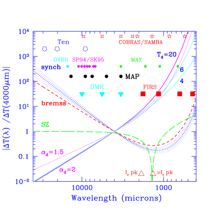
Figure 2: The flat spectrum in thermodynamic temperature predicted for primary anisotropies is contrasted with the spectral signatures for other sources of anisotropy (normalized at 4 mm): SZ anisotropies (long-dashed, with a sign change at $1300~{}\mu{\rm m}$); bremsstrahlung (short-dashed); synchrotron (dotted), with index vvarying from $p_{s}=0.5$ to $0.9$ (intensity $I_{\nu}\propto\nu^{-p_{s}}$); and dust (with index $\alpha_{d}=2$ as indicated by a two-temperature fit to COBE), both the usual Galactic dust at 20 K (heavy solid) and dust at 6 K and 4 K (light solid lines, which could represent a cold Galactic component or, e.g., 30 K dust radiating at redshift $\sim 5$); a shallower, less physically-motivated, $\alpha_{d}=1.5$ dust opacity law for the 20K grains is also shown, appropriate for the single-temperature COBE fit. The frequency bands which various experiments probe are indicated, in particular the proposed bands for the NASA (MAP) and ESA (COBRAS/SAMBA) all-sky satellite experiments. There is a minimum of the Galactic foregrounds at about 90 GHz, the highest frequency COBE channel.

2 CMB Distortions and Energetic Constraints

In this section, I review the impact of spectrum observations on structure formation issues. We know from FIRAS that the CMB is well fit by a blackbody with $T\approx 2.728\pm 0.004$ K over the region from $5000\mu{\rm m}$ to $500\mu{\rm m}$ [11], a number compatible with the 1990 COBRA rocket experiment of Gush et al. [20] covering the same band, and also with ground based measurements at centimetre wavelengths — although there is still room for significant spectral distortion longward of 1 cm. We must rely on indirect arguments based on primordial nucleosynthesis to constrain exactly when this photon entropy in our Hubble patch came into being, and whether this injection of energy would have a direct impact on short-distance structure formation. Energy injection prior to $z_{Pl}\approx 10^{6.9}\Big{(}{\Omega_{B}{\rm h}^{2}/0.01}\Big{)}^{-0.39}$ is redistributed into a Planckian form: $z_{Pl}$ defines the redshift of the cosmic photosphere. There have been heroic efforts to explain the CMB as starlight processed through exotic forms of dust (in particular long conducting needles) that would have happened much later. The observables from these models have never been fully worked out (see, e.g., [1]), but they are severely challenged by the absence of spectral distortions and the high degree of anisotropy required.

Between $z_{Pl}$ and $z_{BE}\approx 10^{5.6}\big{(}{\Omega_{B}{\rm h}^{2}/0.01}\big{)}^{-1/2}$ injected energy is redistributed into a Bose-Einstein shape characterized by a chemical potential, which FIRAS constrains to be [11] $|\mu_{\gamma}|/T_{\gamma}<0.9\times 10^{-4}$ (95%  CL), translating to a limit on energy of ${\delta E_{BE}/E_{cmb}}\mathrel{\hbox to0.0pt{\lower 3.0pt\hbox{$\mathchar 536\relax$}\hss}\raise 2.0pt\hbox{$\mathchar 316\relax$}}6.4\times 10^{-5}$ in this redshift range. Below $z_{y}\approx 10^{5}\big{(}{\Omega_{B}{\rm h}^{2}/0.01}\big{)}^{-1/2}$ the Compton $y$-distortion formula holds, giving a unique signature to distortions, negative for frequencies below $218$ GHz, positive above, and a stringent limit on the Compton-cooling energy loss from hot gas, ${\delta E_{Compton\ cool}/E_{cmb}}=4y<6.0\times 10^{-5}$ (95% CL). If there is no recombination, there is a constraint from the $y$-distortion on how early reheating of the Universe can have occurred: $z_{max,reh}\approx 10^{3.7}\big{(}{\Omega_{B}{\rm h}/0.02}\big{)}^{-2/3}\Omega_{nr}^{1/3}$ [21, 22, 1], but it is not very restrictive for the low $\Omega_{B}$ favoured by standard Big Bang nucleosynthesis and can be avoided if one can sustain a temperature of the cooling electrons to be nearly the CMB temperature.

Compton cooling has been observed in more than two dozen massive clusters of galaxies above the $5$-$\sigma$ level, including one at redshift 0.545, which tells us that the CMB existed by at least that redshift. With likely experimental sensitivity increases, the SZ effect may eventually offer a more powerful probe of the cluster distribution than $X$-ray observations do: instead of being a projection of the square of the baryon density, it is a projection of the electron pressure and the decrease in signal with redshift is only a consequence of cluster evolution, not dimming by distance. Combining the SZ and $X$-ray observations is one of the main paths to $H_{0}$ (and in principle $q_{0}$), but is so far more confusing than enlightening, with values ranging from small (e.g., $H_{0}=38\pm 17$ for Abell 2218) to large ($74\pm 29$ for COMA); the hope is that a well-selected sample of clusters may help to reduce the biases.

The integrated contribution of Compton-cooling from clusters and groups is not expected to be large for models of structure formation that reproduce the cluster X-ray temperature distribution function. For example [23], for variants of adiabatic dark-matter dominated $\Omega=1$ models with $\Omega_{B}\ll\Omega$, ${\rm h}=0.5$ and nearly scale-invariant initial conditions, the estimated value depends sensitively on $\sigma_{8}$, the linear amplitude of density fluctuations on the cluster-scale $8{\rm\,h^{-1}Mpc}$, and somewhat on the local curvature of the density fluctuation spectrum on cluster-scales: with $\sigma_{8}=0.7$, a hot/cold hybrid model with $\Omega_{\nu}=0.3$ gives $\bar{y}\sim 0.3\times 10^{-6}(\Omega_{Beff}/0.05)$, a tilted CDM model with $n_{s}=0.8$ gives $\sim 0.5\times 10^{-6}(\Omega_{Beff}/0.05)$, with a similar value obtained for a $n_{s}=1$ model. Lowering $\sigma_{8}$ gives values well below $10^{-6}$, but also not enough high temperature clusters; raising it gives too many high $T_{X}$ clusters (raising $\sigma_{8}$ to unity still gives only $\bar{y}\sim 1.6\times 10^{-6}(\Omega_{Beff}/0.05)$). Here $\Omega_{Beff}$ takes into account the possible segregation of baryons from mass in clusters, modifying the value to be used over the primordial $\Omega_{B}$. There is an even smaller effect associated with nonlinear Thompson scattering from the hot gas in the moving clusters. Nonetheless, the non-Gaussian pattern of Compton-cooling secondary anisotropies is accessible to experiment and will be a foreground to remove in future CMB anisotropy experiments [8].

The FIRAS limit on general secondary backgrounds (without a unique signature like BE or $y$ distortions) is ${\delta E/E_{cmb}}(500-5000\mu{\rm m})<0.00025$ ($1\sigma$ CL). If pregalactic dust, or dust in primeval galaxies, exists, it will absorb higher frequency radiation (UV and optical) and down-shift it into the infrared (e.g., [24]); combined with the redshift, a sub-mm background is expected but, with FIRAS, is now quite strongly constrained. The radiation could be largely shortward of $500\mu{\rm m}$: the peak in the $\nu I_{\nu}$ curve occurs at $\lambda_{pk}\approx 96(1+z)(30{\rm K}/T_{d})$ for $\alpha_{d}=2$ dust, which could be around $200\mu{\rm m}$ if the dust is hot (which seems reasonable) or the redshift of bulge/elliptical formation is low. The FIRAS constraint then applies only to the tail of emission. There is a tentative identification of a sub-mm background in the FIRAS data [18] in the range $\sim 200-1000~{}\mu{\rm m}$, with energy $\delta E/E_{cmb}\sim 10^{-3}$ longward of $\sim 400~{}\mu{\rm m}$, which partly mimics the Galactic contribution (and could be partly due to cold high latitude Galactic dust [17]). There are also residuals after source subtractions in the DIRBE data which could be interpreted as a cosmological infrared background at shorter ($\sim 1-200~{}\mu{\rm m}$) wavelengths at the $\delta E/E_{cmb}\sim 10^{-2}$ level [25]. These constraints on energy injection should be contrasted with plausible sources: For example, the nuclear energy output of stars with efficiency $\epsilon_{nuc}$ radiating at redshift $z_{*}$ with an abundance $\Omega_{*}$ relative to the CMB is ${E_{*}/E_{cmb}}\approx 0.03\big{(}{\Omega_{*}{\rm h}^{2}/0.001}\big{)}\ {[5/(1+z_{*})]}\ [{\epsilon_{nuc}/0.004}]$. Massive stars in the $10$–$100{\rm\,M_{\odot}}$ range have $\epsilon_{nuc}\sim 0.004(M/100{\rm\,M_{\odot}})^{0.5}$, saturating at 0.004 above $>100{\rm\,M_{\odot}}$ (the Very Massive Object range). $E_{*}$ has been used to constrain the role pregalactic black holes from VMO precursors could have played as dark matter. The massive star $E_{*}$ is also tied to the heavy elements $Z_{ej}M$ they eject in supernova explosions. If the supernovae contribute a mean metal fraction $Z$ to a gas of density $\Omega_{gas}$, ${E_{preSN\,*}/E_{cmb}}\approx 0.0008[{Z/10^{-3}}]{[\Omega_{gas}{\rm h}^{2}/0.01]}[{Z_{ej}/0.2}]\big{(}{M/20{\rm\,M_{\odot}}}\big{)}^{0.5}$. Relaxation of the stringent energetic constraints is possible if either the energy was not reprocessed by dust (and so would reside in the near infrared where the DIRBE constraints are not nearly as strong [25]) or the dust was so hot that even with redshift effects it was shortward of $500\mu m$.

As Ikeuchi and Ostriker originally emphasized, a predominantly hydrodynamic explanation for cosmic structure development is a perfectly reasonable extrapolation of known behaviour in the interstellar medium to the pregalactic medium. However the Compton cooling limit constrains the combination $f_{exp}\big{(}{R_{exp}/50{\rm\,h^{-1}Mpc}}\big{)}^{2}$ of filling factor $f_{exp}$ and bubble formation scale $R_{exp}$ to be $\mathrel{\hbox to0.0pt{\lower 3.0pt\hbox{$\mathchar 536\relax$}\hss}\raise 2.0pt\hbox{$\mathchar 316\relax$}}[(\Omega_{B}{\rm h}/0.02)\Omega_{nr}^{1/2}]^{-1}$ (e.g., [1]). Further, if supernova explosions were responsible for energy injection, one expects that the presupernova light radiated would be much in excess of the explosive energy (more than a hundred-fold), which would lead to much stronger restrictions on the model; and if the supernova debris is metal-enriched, the allowed amount of metals poses an even stronger constraint. (One may also argue that the specific tapestry that we see is too close to what straightforward gravitational instability predicts to warrant consideration of a purely hydrodynamical model; i.e., that the explosive effects might be largely masked by subsequent gravitational instability. What does seem inevitable is that there will be a more limited local hydrodynamics role around collapsed objects.)

3 Theoretical Issues and Sample Primary Power Spectra; COMBA

The development of spectral distortions or angular anisotropies in the microwave background is described by radiative transfer equations for the photon distribution function, which are coupled to Einstein’s equations for the gravitational field and to the hydrodynamic and transport equations for the other types of matter present. The primary spectra are calculated by solving for each mode $\in\{$adiabatic scalar, isocurvature scalar, vector or tensor$\}$ the linearized Boltzmann transport equation for photons (including polarization) and relativistic or light neutrinos, coupled to the equations of motion for baryons and cold dark matter, and the perturbed gravitational metric equations, possibly in the presence of vacuum energy or mean curvature. This is a well developed art the techniques for which have been described elsewhere (e.g., [1]) and will not be elaborated upon here. In homage to the high precision future that CMB experimentalists will provide for us, a large consortium of theorists who have developed computer codes to attack this problem fully or in various fast-computation approximations have combined under the acronym COMBA to deliver accurate validated calculations of ${\cal C}_{\ell}$’s to the cosmological community [26].

I now sketch the ${\cal C}_{\ell}$ terrain in inflation-inspired models as the parameters defining the structure formation model are varied. Samples are shown in Figs. 1,3. The “standard” scale invariant adiabatic CDM model ($\Omega=1$, $n_{s}=1$, ${\rm h}=0.5$, $\Omega_{B}=0.05$) with normal recombination shown in Fig. 1 and repeated in each of the panels of Fig. 3 illustrates the typical form: the Sachs-Wolfe effect arising from gravitational potential fluctuations dominating at low $\ell$, followed by rises and falls in the first and subsequent Doppler (or acoustic) peaks, arising from a combination of photon compression and rarefaction and electron flow at photon decoupling, with an overall decline due to destructive interference across the photon decoupling surface and damping by shear viscosity in the photon plus baryon fluid. A CDM model with very early reionization (at $z>200$) shows no Doppler peaks, a result of destructive interference from forward and backward flows across the decoupling region, illustrating that the “short-wavelength” part of the density power spectrum can have a dramatic effect upon ${\cal C}_{\ell}$, since it determines how copious UV production from early stars was. Lower redshifts of reionization still maintain a Doppler peak, but are suppressed relative to the standard CDM case (as illustrated by the $z_{reh}\sim 30$ model in Fig. 1 and in Fig. 3(e)).

Figs. 1,3 include adiabatic scalar and tensor contributions. The relative magnitude of each is characterized by either the ratio of the quadrupole powers, $r_{ts}={\cal C}_{2}^{(T)}/{\cal C}_{2}^{(S)}$, or the ratio of the dmr band-powers $\tilde{r}_{ts}={\langle{\cal C}_{\ell}^{(T)}\rangle}_{dmr}/{\langle{\cal C}_{\ell}^{(S)}\rangle}_{dmr}$. For the scale invariant cases, $r_{ts}$ is taken to vanish.

A simple variant of CDM-like models is to tilt the initial spectrum. The scalar tilt $\nu_{s}=n_{s}-1$ is defined in terms of the index $n_{s}$, which is one for scale invariant adiabatic fluctuations. There is a corresponding tilt which characterizes the initial spectrum of gravitational waves which induce primary tensor anisotropies, $\nu_{t}=n_{t}+3$, where $n_{t}$ is $-3$ for a scale invariant spectrum. Inflation models give $\nu_{t}<0$ and usually give $\nu_{s}<0$. For small tensor tilts, $r_{ts}\approx-6.9\nu_{t}$ and $r_{ts}\approx 1.3\tilde{r}_{ts}$ are expected (with corrections given by eq. 10). For a reasonably large class of inflation models $\nu_{t}\approx\nu_{s}$, but in some popular inflation models $\nu_{t}$ may be nearly zero even though $\nu_{s}$ is not. Figs. 1 and 3(a) show ${\cal C}_{\ell}^{(S)}+{\cal C}_{\ell}^{(T)}$ derived for tilted cases when $\nu_{t}=\nu_{s}$ is assumed to hold. Fig. 1 shows explicitly the contribution that ${\cal C}_{\ell}^{(T)}$ makes in one example. The tilt indices, especially $\nu_{s}$, can also be complex functions of $k$ in inflation models in which scale invariance is radically broken (e.g., [27]), in which case the ${\cal C}_{\ell}$ reflect the added complexity.

Spectra for hot/cold hybrid models with a light massive neutrino look quite similar to those for CDM only, as Fig. 3(f) shows [41, 42, 43]. This is true even for pure hot dark matter models [44].

The dotted ${\cal C}_{\ell}$ in Fig. 1 also has a flat initial spectrum, but has a large nonzero cosmological constant in order to have a high $H_{0}$, in better accord with most observational determinations. As one goes from $\ell$=2 to $\ell$ =3 and above there is first a drop in ${\cal C}_{\ell}$ [28], a consequence of the time dependence of the gravitational potential fluctuations (the integrated Sachs-Wolfe effect). Other nonzero $\Lambda$ examples are given in Fig. 3(d).

Open models like the $H_{0}=60$ one shown in Fig. 1 have a nontrivial late-time integrated Sachs-Wolfe effect, like the $\Omega_{\Lambda}\neq 0$ models do, but there is also a direct effect of the curvature on the mode function evolution, which serves to focus the structure to a smaller angular scale ($\sim\Omega_{nr}^{1/2}$) than in the $\Omega_{curv}\equiv 1-\Omega_{tot}=0$ case. Of course whatever mechanism generated the ultra-large-scale mean curvature may well have had associated with it strong fluctuations on observable scales, so much so that this is an argument against large mean curvature because of the absence of such effects in the CMB. Even if the background curvature is determined by an entirely different mechanism, it should influence the fluctuation generation mechanism. An open issue in open models has always been what is a natural shape for the spectrum for $k$ near $d_{curv}^{-1}\equiv H_{0}\Omega_{curv}^{1/2}$. Power laws in $kd_{curv}$, $\sqrt{(kd_{curv})^{2}-1}$ etc. have often been adopted but if the fluctuation generation mechanism is quantum noise in inflation, there is a natural adiabatic spectrum expected which is a simple generalization of the nearly scale invariant spectra of $\Omega_{curv}=0$ inflation models [29, 30, 31]. Fortunately for $\ell\gg 2\Omega_{nr}^{-1}\Omega_{curv}^{1/2}$ this issue is not a factor, so that intermediate and small angle predictions are relatively unambiguous.

Inflation-based models with isocurvature rather than adiabatic initial conditions are strongly ruled out by the CMB data if they are nearly scale invariant [32, 33], but could contribute at a subdominant level to the adiabatic fluctuations. Even allowing for arbitrarily broken scale invariance in the initial fluctuation spectra, the allowed region for pure isocurvature baryon or CDM models has been shrinking fast as the data has improved.

Defect models have (knot-like or string-like) localized topological field configurations acting as isocurvature seed perturbations to drive the growth of fluctuations in the total mass density. On large angular scales the defect models lead to a similar nearly scale-invariant spectrum for ${\cal C}_{\ell}$ as for inflation-inspired adiabatic perturbation models [34, 35, 36, 37, 38, 39]. On smaller scales, the spectra are sufficiently different from adiabatic inflation-inspired spectra to sharply test these competing pictures of cosmic structure formation in the next generation of CMB experiments. The non-Gaussian nature of defect-induced anisotropies also adds another point of differentiation among the models.

The angular power spectra generally differ substantially as a function of multipole $\ell$ so that even with the experimental results we expect in the very near future major swaths of cosmological parameter space can be ruled out. However, different combinations of the parameters $n_{s},r_{ts},\Omega_{B},\Omega_{\Lambda}$ etc. can lead to nearly identical spectra [3], as Fig. 3(f) illustrates. Superposed upon the spectra in Fig. 3 are theoretical band-powers derived for a variety of anisotropy experiments. Fig. 3 also shows 10% 1-sigma error bars: COBE achieved 14% errors with 4 years of data; to achieve this with smaller angle experiments one needs to have about the same number of pixels as COBE, but scaled to the beam size hence covering a smaller region of the Universe. So far none of the smaller angle data sets have the 650 or so fwhm-sized pixels COBE does, but this is the stage we are now entering [59].

As noted before, even if there were idealized perfect all-sky coverage with noise-free versions of the experiments of Fig. 3, there would still be cosmic variance errors on the band-powers, but these are $\sim{\langle\ell\rangle}^{-1}$ [40], much smaller than the size of the points. Thus it appears that by using (perfect) CMB experiments which are sensitive to a wide range of angular scales, we can distinguish even among the nearly degenerate theoretical models shown, and be able to measure the parameters that define the variations in these models. A closeup view of examples of how we can measure very fine differences in models is shown in Fig. 4, using the detector sensitivities and long observing times that satellite experiments now currently feasible can achieve [6, 8].

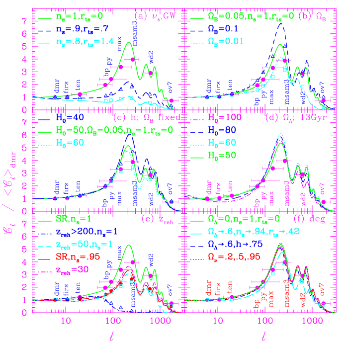
Figure 3: (previous page) Spectra for a variety of inflation-inspired models, normalized to the COBE band-power. Theoretical band-powers for various experimental configurations are placed at ${\langle\ell\rangle}_{W}$, horizontal error bars extend to the $e^{-1/2}\overline{W}_{max}$ points. Unless otherwise indicated, $\Omega_{B}{\rm h}^{2}$=0.0125, ${\rm h}$=0.5, $n_{s}$=1; when the gravity wave contribution is nonzero, $\nu_{t}$=$\nu_{s}$ is assumed (and $r_{ts}\equiv{\cal C}_{2}^{(T)}/{\cal C}_{2}^{(S)}$ is $\sim-7\nu_{t}$). The untilted $n_{s}$=1, $r_{ts}$=0 model is repeated in each panel (solid line). (a) CDM models with variable tilt $n_{s}$. (b) $n_{s}$=1 models with $\Omega_{B}{\rm h}^{2}$ changed, ${\rm h}$ fixed. (c) $n_{s}$=1 models, with $\Omega_{B}{\rm h}^{2}$ changed, $\Omega_{B}$ fixed. (d) $n_{s}$=1 models with fixed age, 13 Gyr, but variable $H_{0}$ and $\Omega_{\Lambda}=1-\Omega_{cdm}-\Omega_{B}$ (.92,.79,.43,0 for 100,80,60,50). (e) CDM models with very early reionization at $z_{reh}\mathrel{\hbox to0.0pt{\lower 3.0pt\hbox{$\mathchar 536\relax$}\hss}\raise 2.0pt\hbox{$\mathchar 318\relax$}}150$ (equivalent to ‘no recombination’), and later reionization at $z_{reh}$=30,50 are contrasted with standard recombination (SR). The $z_{reh}$=50 spectrum is close to the $n_{s}$=0.95 spectrum with SR (thin, dot-dashed): the moderate suppression if $20\mathrel{\hbox to0.0pt{\lower 3.0pt\hbox{$\mathchar 536\relax$}\hss}\raise 2.0pt\hbox{$\mathchar 316\relax$}}z_{reh}\mathrel{\hbox to0.0pt{\lower 3.0pt\hbox{$\mathchar 536\relax$}\hss}\raise 2.0pt\hbox{$\mathchar 316\relax$}}150$ can be partially mimicked by decreasing $n_{s}$ or increasing ${\rm h}$. (f) Sample cosmologies with nearly degenerate spectra and band-powers. Dashed curve: increasing $\Omega_{\Lambda}$ is compensated by increasing ${\rm h}$. Dot-dashed curve: tilting to $n_{s}$=0.94 ($\tilde{r}_{ts}$=0.42) is compensated by increasing $\Omega_{\Lambda}$ to 0.6. The dotted hot/cold model curves [43] (with $\Omega_{\nu}$ indicated) are nearly identical to the standard CDM one, but even these few percent differences can be distinguished in principle by satellite all-sky experiments with currently available detector technology.

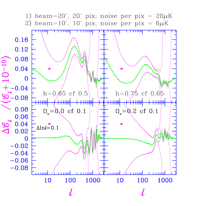
Figure 4: This shows the ability of satellites to measure cosmic parameters to high accuracy. The relative difference of the power spectrum in question from a comparison spectrum (both normalized to the 4-year dmr (53+90+31)A+B COBE maps) are shown so that the few percent deviations can be clearly seen over the entire $\ell$ range. The lighter lines are $1-sigma$ error bars for all-sky coverage (averaged over the smoothing width shown, with $\textstyle{1\over 2}\Delta\ln\ell=0.05$) and include cosmic variance (dominant at low $\ell$) and pixel noise at $20\mu{\rm K}$ or $6\mu{\rm K}$ (dominant at high $\ell$), with the very rapid growth relative to the theory curve at high $\ell$ coming from the finite beam-size (with the fwhm indicated, corresponding to a Gaussian filter in multipole space of $\ell_{s}=404$ and $\ell_{s}=809$ respectively). The first choice corresponds to the NASA satellite experiment MAP, the second choice to the ESA mission COBRAS/SAMBA, assuming the entire sky is usable (errors scaling $\propto f_{sky}^{-1/2}$). The ultimate accuracy achievable will depend upon the decontamination of the primary signal of non-Gaussian Galactic synchrotron, bremsstrahlung and dust signals. The models shown all have a uniform age of 13 Gyr, $\Omega_{cdm}+\Omega_{m\nu}+\Omega_{\Lambda}+\Omega_{B}=1$, $\Omega_{B}{\rm h}^{2}=0.0125$, $n_{s}=1$ and no gravity wave contribution. Notice the scale change for the hot/cold model panels. (One species of massive neutrino was adopted for these two cases.)

4 Secondary Anisotropy Sources

Reionization and Primary CMB Anisotropies: An important issue associated with the early energy injection described in § 2 is what impact it will have on the primary anisotropies of the CMB. The physical processes important in the recombination of the primeval plasma have been well understood since shortly after the discovery of the CMB. The comoving width of the region over which decoupling takes place if there is normal recombination is only $(5-10)\Omega_{nr}^{-1/2}{\rm\,h^{-1}Mpc}$, where $\Omega_{nr}$ is the density in non-relativistic particles (CDM, baryons); the viscous damping scale of the photon-baryon fluid prior to recombination is slightly less. The associated angular scale can be characterized by a multipole number, $\ell\sim 1000$, above which anisotropies are strongly damped (Fig. 1). The associated natural ‘coherence’ angle, $\sim 10^{\prime}$, defines which experiments are most useful to do if we wish to probe the moment when the photons were first released to freely propagate from their point of origin to us, without much further modification, apart from some gravitational redshifts, some lensing, and possibly some scattering from hot gas.

The main effect that reionization of the Universe has on anisotropies is to lower their amplitude by a factor $\Delta T/T\propto e^{-\zeta_{C}}$, where $\zeta_{C}$ is the optical depth to Thompson scattering. If $z_{reh}$ is the reionization redshift and $z_{\zeta_{C}=1}\approx 10^{2.1}\big{(}{\Omega_{B}{\rm h}/0.02}\big{)}^{-2/3}\,\Omega_{nr}^{1/3}$ is the redshift one would need to reionize by to get a Thompson depth of unity, then $\zeta_{C}=[(1+z)/(1+z_{\zeta_{C}=1})]^{3/2}$. With standard Big Bang nucleosynthesis values for $\Omega_{B}$, getting $z_{\zeta_{C}=1}$ much below 100 seems unlikely. $z_{reh}$ is presumably the redshift by which the first nonlinear objects form in sufficient abundance to allow enough massive star formation to occur to cause pregalactic HII regions to overlap, a quantity largely determined by the short-distance density fluctuation power in the structure formation theory in question, but subject to many uncertainties: the entities which form may well be rather fragile with a small binding energy, easily disrupted by the massive stars they generate; on the other hand, the amount of nonlinear gas could be amplified by the explosion of such stars sweeping up shells of gas far from the parent object. Thus $z_{reh}$ depends upon how rare the ionization-generators can be. For inflation-based CDM models and variants with light massive neutrinos or nonzero $\Lambda$, $z_{reh}$ values ranging from 5 to 60 seem plausible, hence $\zeta_{C}$ ranges from negligible to substantial, $\mathrel{\hbox to0.0pt{\lower 3.0pt\hbox{$\mathchar 536\relax$}\hss}\raise 2.0pt\hbox{$\mathchar 316\relax$}}1/3$, but not so large as to fully erase anisotropies, which would occur on scales below $\tau_{dec}/\pi$, where $\tau_{dec}$ is the horizon scale at photon decoupling, corresponding to $\ell\sim 100$ for the “standard” CDM model. See Figs. 1 and 3(e) for $z_{reh}\sim 30,50$ examples.

In isocurvature baryon models with (nearly) white noise initial conditions popular in the late seventies, the first objects collapse at $z\sim 300$, making reionization easy, and, indeed, expected. Thus, large viscous damping is expected. However, one can still have a peak in ${\cal C}_{\ell}$ at $\ell\sim 200$ for open models, essentially because the modified angle-distance relation in curved universes shifts power to higher $\ell$. Early ionization seems plausible, but by no means certain, in models in which there are isocurvature seeds, such as in texture models [36].

Reionization and Quadratic Nonlinearities in Thomson Scattering: These can sometimes dominate over the first-order anisotropies if the latter are strongly damped and there is early ionization. Even if there is early reionization in nearly scale invariant models, there is generally not sufficient power on small length scales for this Vishniac effect [45] to be important. Thus it can usually be ignored in inflation-based models. This is not so for isocurvature baryon models [33] in which the initial spectral index $n_{is}$, considered a free parameter, is between –1 and 0 on phenomenological grounds. Such a steeply rising spectrum implies short-distance effects are very important, and give predicted sizable signals in e.g., the ovro and VLA window of Fig. 1.

The Rees-Sciama Effect: In flat $\Omega_{nr}=1$ models, the gravitational potential fluctuations have constant amplitude in the linear phase of evolution. Weak (or strong) nonlinear evolution induces time dependence in $\Phi_{N}$ which induces anisotropy by an integrated Sachs-Wolfe effect. For inflation-inspired models this turns out to be a very small correction and can be largely ignored.

The Influence of Weak Gravitational Lensing on the CMB: Another nonlinear effect (on the distribution function) is gravitational lensing which bends, focusses and defocusses the CMB photons as they propagate from decoupling through the clumpy medium to us. Given the difficulties that astronomers have had detecting lensing, with the best observations coming from clusters of galaxies, it may seem obvious that the effect on the $\sim 10^{\prime}$ coherence scale typical for primary CMB anisotropies is likely be quite small; and this is what (most of) the people who have investigated the effect have found. Lensing conserves the total angular power, it just rearranges it, by smoothing the Doppler peaks. The typical range in $\ell$ over which the power is spread in $\Delta\ell/\ell$ is basically the weak-lensing shear, about 10% to 20% or so at a few arcminutes, depending upon the model [46]; this is in agreement with the levels estimated by people advocating using the influence of weak-lensing on the ellipticities of faint galaxy images to determine the mass density power spectrum e.g., [47].

Sunyaev-Zeldovich Fluctuations and the Moving Cluster Effect: The SZ effect has been discussed in § 2. The moving cluster effect is the nonlinear Thomson scattering of the CMB photons from plasma confined to clusters, moving with it. It is predicted to be quite a bit smaller than the SZ anisotropy level, and as can be seen from Fig. 1 the contribution of SZ from clusters is small relative to the primary anisotropy power [23]. However, the distribution is non-Gaussian, concentrated in the pressure-peaks in the medium, especially the clusters. This means a search for the ambient SZ-effect (where the SZ sources are not known beforehand) could be very promising [8].

Starbursting Primeval Galaxies: As discussed in § 2 on CMB distortions and energetic constraints, the prospects for seeing these with sub-mm telescopes probing tens of arcseconds (e.g. SCUBA filter in Fig. 1) seem quite good [24, 1].

5 Anisotropy Experiments and their Band-Powers

The importance of the large-angle COBE dmr [48, 49] detection for testing theories of cosmic structure formation can hardly be overstated. Smaller angle experiments are now also achieving results that can be combined with COBE to constraint model parameters. In this section, I review the experiments.

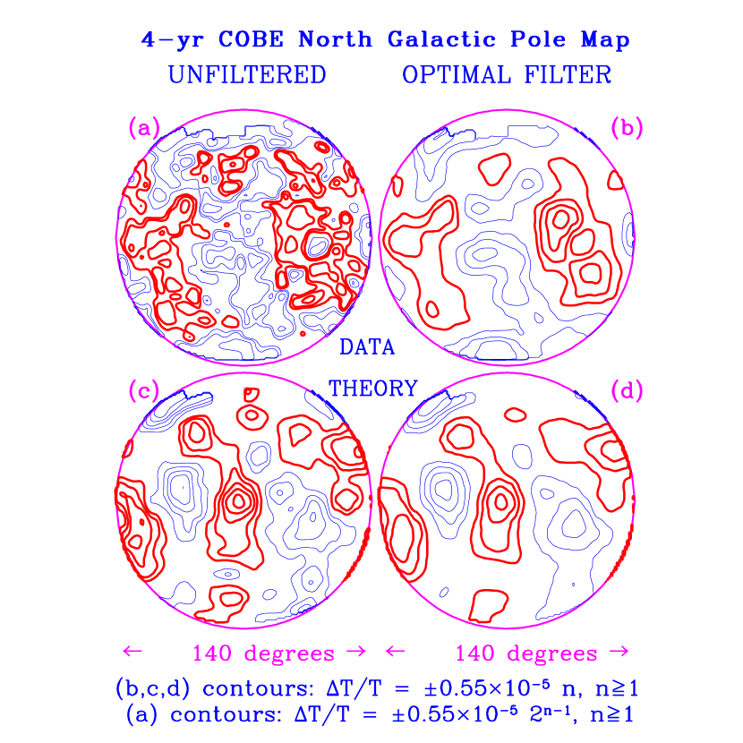
Figure 5: $140^{\circ}$ diameter maps centered on the North Galactic Pole are shown for a realization of a CDM ${\cal C}_{\ell}$–spectrum convolved with the dmr beam in (c). No noise has been added. This is how the primary sky would appear in a $n_{s}=1$ CDM Universe with $\sigma_{8}=1.2$ (or in a $\Omega_{m\nu}=0.2$ hot/cold universe with $\sigma_{8}=0.8$), the most likely values for the dmr data. This is contrasted with the 4-year dmr (53+90+31)a+b data map shown in (a) and the map after the data has undergone optimal signal-to-noise filtering in (b) (using the same ${\cal C}_{\ell}$-shape and amplitude for the filter). The statistically significant features are also seen in each of the dmr channel maps after optimal filtering (which preferentially removes high angular frequencies, more so for noisier maps). Thus, to compare, (d) shows the theoretical realization after passing (c) through the same optimal filter used for (b); the average, dipole and quadrupole of the full $|b|>20^{\circ}$ sky were also removed, an effective low $\ell$-filter – if they stay in, the maps look similar to the unfiltered theory maps except small scale smoothing leads to loss of the higher contour levels. Note that the contours are linearly spaced at $\pm 15n~{}\mu{\rm K}$ for all but (a), for which the spacings are $\pm 15,30,60,120~{}\mu{\rm K}$. The maps have been smoothed by an additional $1.66^{\circ}$ Gaussian filter.

The COBE data stream gives temperature differences in pixel pairs separated by $60^{\circ}$, but an inversion yields 6 maps, for the $A$ and $B$ channels of the 3 frequencies shown in Fig. 2, 31, 53 and 90 GHz. Figure 5 compares an optimally filtered map of COBE’s data with what a scale invariant $\Omega=1$ dark matter dominated model would look like under the same filtering.

The $\ell=2$ power uses the 4-year quadrupole value [49, 50], determined from high Galactic latitude data. It is the multipole most likely to have a residual Galactic signal contaminating it, possibly destructively, and the “systematic” error, the dashed addition to the statistical error bar (solid), reflects this. The two heavy points at $\ell\sim 7$ are band-powers derived for the 4-year dmr 53+90+31 GHz “$A$+$B$” maps [12, 1, 13], the solid point assuming a $\nu_{\Delta T}=0$ spectrum, the open marginalizing over all possible $\nu_{\Delta T}$, where $\nu_{\Delta T}$ is defined by eq.(5).

The two points at $\ell\sim 10$ are for the firs map [52], solid with the restriction $\nu_{\Delta T}=0$, open with $\nu_{\Delta T}$ allowed to float. The coverage of the firs experiment is much less extensive and more inhomogeneous over the observed patch than for dmr: it was a balloon experiment (taking useful data for only about 5 hours) with bolometer detectors probing the 4 frequency channels shown in Fig. 2. Only the 170 GHz channel has been fully analyzed. The pixel size, $1.3^{\circ}$, and the beam-size, $\ell_{s}\approx 34$ (a $3.9^{\circ}$ fwhm beam) are half the COBE values. The firs map has a positive cross-correlation with dmr [52]. The band-powers of dmr and firs are quite comparable, almost independent of degree of the signal-to-noise filtering and which frequencies are probed. And it is only weakly dependent upon the slope $\nu_{\Delta T}$ (as the formula for ${\langle{\cal C_{\ell}}\rangle}_{dmr}$ as a function of $\nu_{\Delta T}$ given by eq.(12) shows).

The effective slope of the standard CDM model is $\nu_{\Delta T}\approx 0.15$ over the dmr band; variation in $\Omega_{B}$ and $H_{0}$ does not change this very much. dmr and firs have enough coverage in $\ell$-space that one can estimate the spectral index from the data as well by Bayesian means. If there is no filtering the 53+90+31 GHz ‘$A$+$B$’ index is $\nu_{\Delta T}$ is $0.07\pm 0.28$ for dmr; firs gives a steeper index, $0.6^{+0.7}_{-0.8}$, but the one sigma error bar encompasses $0$ and there is clearly a small angle residual ‘noise’ driving the higher values [40, 1]. When CDM models are marginalized over $\sigma_{8}$ the preferred dmr index is $n_{s}=1.02^{+.23}_{-.25}$ for the case with no gravity waves ($\nu_{t}=0$), and $n_{s}=1.02^{+.23}_{-.18}$ with gravity waves ($\nu_{t}=\nu_{s}$) [13]. Band-powers for specific $\ell$ ranges also show the nearly flat character for ${\cal C}_{\ell}$ (light open points at $\ell\sim 4,8,16$ from [51]).

The Tenerife point [53] at $\ell\sim 20$ uses combined 15 and 33 GHz data. The amplitude is compatible with dmr and firs, with CDM-like models, and also have features in common with dmr.

We now come to the crowded region from two degrees to half a degree. The next two experiments are the South Pole HEMT experiments of the UCSB group and the Saskatchewan (Big Plate) HEMT experiment of the Princeton group. The lower open circle is from a joint 4-channel analysis of the 9 and 13 point sp91 scans [54, 55, 40, 13] (with the individual 9 point and 13 point values given in the lower panel). The upper solid point is for a simultaneous analysis of all channels of the sp94 data [56, 13], with separate values for the Ka ($\sim 30~{}{\rm GHz}$) and Q ($\sim 40~{}{\rm GHz}$) HEMT bands (Fig. 2) in the lower panel. The solid triangle in the upper panel is the sk93 result [57]; the big solid circle at $\ell\sim 80$ in the lower panel is the sk93+94 result (with calibration uncertainties adding another 14% error to the statistical error shown). The nearness of the sp94, sk93 and sk93+94 band-powers, and the demonstration for both experiments that the preferred frequency dependence is nearly flat in $\Delta T/T$ and many sigma away from bremsstrahlung or synchrotron, the expected contaminants in this 30-40 GHz range, lend confidence that the spectrum in the $\ell\sim 60$–$80$ region has really been determined; and it looks quite compatible with the COBE-normalized CDM spectrum: sp94 gives $\sigma_{8}=1.26^{+.37}_{-.27}$, and sk93+94 gives $\sigma_{8}=1.21^{+.24}_{-.19}$ [13], very close to the dmr value $\sigma_{8}=1.20\pm 0.08$ and the firs value $\sigma_{8}=1.27\pm 0.30$. The 5 heavy open circle points probing $\ell$’s ranging from 60 to 400 repeated in the upper and lower panels labelled sk95 are combined sk94+95 results [59]. The estimated 14% error in the overall amplitude because of calibration uncertainties are included. The large $\ell$-space coverage from this one intermediate angle experiment gives a first glimpse of the $\ell$-space coverage that will become standard in the next round of anisotropy experiments.

Python [60], py, the heavy solid curve at $\ell\sim 90$, is sensitive to a wide coverage in $\ell$-space as the horizontal error bars in the top panel indicate. Argo [61], ar, a balloon-borne experiment, is next. The next five points in the lower panel are from the fourth and fifth flights, M4,M5, of the MAX balloon experiment [63, 62]. Because the filters changed with frequency, the points are placed at the average over all max filters. In the upper panel three max4 scans are combined into one data point as are two max5 scans. The lines ending in triangles at $\ell\approx 145$ and 240 denote the 90% limits for the MSAM [64] single (msam2) and double (msam3) difference configurations. A limitation on these balloon experiments is the $\sim 5$ hours over which data can be effectively taken. Planned long duration balloon flights that would circle Antarctica for about a week would allow extensive mapping at high precision to be done, and a number of groups have been proposing designs (e.g., ACE, Boomerang and Top Hat).

The CAT points [65] at $\ell\approx 400$ and 600 represent a very different experimental technique, interferometry. CAT is a 3-element synthesis telescope, probing $\sim 15$ GHz frequencies with a $27^{\prime}$ synthesized beam and a $2^{\circ}$ field-of-view (the fwhm of the individual telescopes). It is a precursor to the larger VSA (Very Small Array), covering a wider frequency range with more telescopes and a larger ($4^{\circ}$) FOV. Two other CMB interferometers are also planned: CBI and VCA. The ovro experiments also probe radio frequencies, but using single dishes. The historically important 1987 ovro 7 point upper limit [66] shown used a 40 meter dish. Detections using as well a 5 meter dish have now been found with ovro and give a value in between the 2 CAT points with about the same amplitude. The open triangle at $\ell\approx 160$ denoting the 95% credible limit for the sp89 9 point scan [67, 79] was also historically important. WhiteDish [68] had a small amplitude filter, a hint of a detection in the $m=1$ mode, and a 95% limit in $m=2$ mode at $\ell\approx 520$, wd2.

6 COBE-normalization of Post-Inflation Fluctuations

For early universe calculations and also to characterize the initial conditions for the photon transport through decoupling, the power in adiabatic scalar fluctuations on scales beyond the Hubble radius is best characterized in terms of quantities which become time-independent. Some examples are the spatial curvature of time surfaces on which there is no net flow of momentum ($\propto\varphi_{com}$), as Chibisov and Mukhanov emphasized long ago [69, 70, 71], the expansion factor fluctuation, $\delta\ln a|_{H*}$, on time surfaces with uniform space creation rate $H_{*}$ [72, 1], and Bardeen, Steinhardt and Turner’s $\zeta$ [73, 74, 27]. An initially scale invariant adiabatic spectrum has $k$-independent power per $d\ln k$ in these variables (for $k/(\bar{H}\bar{a})\ll 1$), while for models with spectral tilt $\nu_{s}$, we have ${\cal P}_{\varphi_{com}}(k)={\cal P}_{\varphi_{com}}(\tau_{0}^{-1})(k\tau_{0})^{\nu_{s}}$, where we use the instantaneous comoving horizon size at the current epoch, $\tau_{0}$, as the normalization point. For CDM-like models (those with $\Omega=\Omega_{nr}=1$ and $\tau_{0}=2H_{0}^{-1}$), these are related to the portion of the dmr band power ${\langle{\cal C}_{\ell}\rangle}_{dmr}$ in the scalar adiabatic mode, ${\langle{\cal C}^{(S)}_{\ell}\rangle}_{dmr}={\langle{\cal C}_{\ell}\rangle}_{dmr}/(1+\tilde{r}_{ts})$, and to the quadrupole power, ${\cal C}^{(S)}_{2}={\cal C}_{2}/(1+{r}_{ts})$, by [1]

$${\cal P}_{\varphi_{com}}(\tau_{0}^{-1})\approx 23.5{\langle{\cal C}^{(S)}_{\ell}\rangle}_{dmr}\ e^{-1.99\nu_{s}(1+0.1\nu_{s})}\approx 23.6{\cal C}^{(S)}_{2}\ e^{-1.1\nu_{s}}\,,$$ (8)

$${\cal P}_{{\varphi}_{com}}(k)\approx{\cal P}_{{\ln a}|_{H*}}(k)\approx{\cal P}_{\zeta}(k)\,\quad{\cal P}_{{\varphi}_{com}}(k)={\cal P}_{\varphi_{com}}(\tau_{0}^{-1})(k\tau_{0})^{\nu_{s}}\,,$$

i.e., about $3\times 10^{-9}$. This relation is very insensitive to variations in ${\rm h}$ and $\Omega_{B}$. For scales of order our present Hubble size, we also have ${\cal P}_{\zeta}\approx{25\over 9}{\cal P}_{\Phi_{N}}\approx{25\over 4}{\cal P}_{(\delta\rho)_{hor}}$, where $\Phi_{N}$ is the perturbed Newtonian gravitational potential and $(\delta\rho)_{hor}$ is the density fluctuation at ‘horizon crossing’, defined by $k\tau=1$.

Quantum noise in the transverse traceless modes of the perturbed metric tensor would also have arisen in the inflation epoch and for many models may have been quite significant [75, 76, 77]. The gravitational radiation power spectrum ${\cal P}_{GW}={\cal P}_{h_{+}}+{\cal P}_{h_{\times}}$ is the sum of the two independent gravitational wave polarizations. It is related to the amplitude of the dmr band power ${\langle{\cal C}^{(T)}_{\ell}\rangle}_{dmr}={\langle{\cal C}_{\ell}\rangle}_{dmr}\tilde{r}_{ts}/(1+\tilde{r}_{ts})$ and to the quadrupole ${\cal C}^{(T)}_{2}$ by

$${\cal P}_{GW}(\tau_{0}^{-1})\approx 17.6{\langle{\cal C}^{(T)}_{\ell}\rangle}_{dmr}\ e^{-1.92\nu_{t}(1+0.1\nu_{t})}\approx 13.4{\cal C}^{(T)}_{2}\ e^{-1.25\nu_{t}}\,,$$

$${\cal P}_{GW}(k)={\cal P}_{GW}(\tau_{0}^{-1})(k\tau_{0})^{\nu_{t}}\,.$$ (9)

The inflation model determines the ratio of ${\cal P}_{GW}(\tau_{0}^{-1})$ to ${\cal P}_{{\varphi}_{com}}(\tau_{0}^{-1})$. It is generally related to the tilt of the gravity wave spectrum, and this can in turn by used to relate the ratio of dmr band-powers (and quadrupoles) to the tilts (for $\Omega_{vac}=\Omega_{curv}=0$):

$${\cal P}_{GW}(\tau_{0}^{-1})/{\cal P}_{{\varphi}_{com}}(\tau_{0}^{-1})=-4\nu_{t}/(1-\nu_{t}/2)\ ;\ \ {\rm hence}$$

$$\tilde{r}_{ts}\equiv{{\langle{\cal C}^{(T)}_{\ell}\rangle}_{dmr}\over{\langle{\cal C}^{(S)}_{\ell}\rangle}_{dmr}}\approx 5.4{(-\nu_{t})\over(1-\nu_{t}/2)}\,e^{-0.07\nu_{t}}\,e^{-1.99(\nu_{s}-\nu_{t})}\,,$$

$${r}_{ts}\equiv{{\cal C}^{(T)}_{2}\over{\cal C}^{(S)}_{2}}\approx 6.9{(-\nu_{t})\over(1-\nu_{t}/2)}\,e^{-0.15\nu_{t}}\,e^{-1.1(\nu_{s}-\nu_{t})}\,.$$ (10)

The tensor tilt is simply related to the deceleration parameter $q=-a\ddot{a}/\dot{a}^{2}$ of the Universe in the inflationary epoch, $\nu_{t}/2\approx 1+q^{-1}$; although $1+q^{-1}$ is the leading term for the scalar tilt, other terms can dominate when the deceleration is near the critical deSitter-space value of $-1$ (e.g., [78]). Thus although $\nu_{t}$ is negative, $\nu_{s}$ may not be.

When assessing the effect of gravity waves on the normalization of the spectrum, it is useful to consider two limiting cases: $\nu_{s}\approx\nu_{t}$, which holds for the widest class of models, including power law and chaotic inflation, and $\nu_{t}\approx 0$, with $\nu_{s}$ arbitrary, which holds for some models such as “natural” inflation.

There are also corrections as one goes away from the $\Omega_{nr}=\Omega_{tot}=1$ models. For example, models with nonzero cosmological constant $\Omega_{vac}$, but $\Omega_{nr}+\Omega_{vac}=1$, have ${\cal P}_{GW}/{\langle{\cal C}^{(T)}_{\ell}\rangle}_{dmr}$ being only weakly dependent upon $\Omega_{vac}$ whereas ${\cal P}_{\zeta}/{\langle{\cal C}^{(S)}_{\ell}\rangle}_{dmr}\propto(1-0.6\Omega_{vac}^{3.5})$ is strongly dependent upon it.

7 Using COBE, FIRS, SP94, SK94, … to fix $\sigma_{8}$

Before the COBE detection, normalization of the density spectrum was done using $\sigma_{8}$, the rms (linear) mass density fluctuations on the scale of $8{\rm\,h^{-1}Mpc}$, or to a biasing factor $b_{g}$ for galaxies, which was usually assumed to obey $b_{g}\sigma_{8}\approx 1$ e.g., [44, 79]. The relation of $\sigma_{8}$ to the initial power spectrum amplitude ${\cal P}_{{\varphi}_{com}}(\tau_{0}^{-1})$ is more sensitive to the specifics of the model, such as type of dark matter, spectral slope, ${\rm h}$, than is the dmr band-power relation given in § 6. Comparing $\sigma_{8}$ estimates from large scale structure observations with the COBE-normalized value is thus extremely important for constraining cosmological parameter space. In this section I present a useful functional form, $\sigma_{8}(\Gamma,\nu_{s},\nu_{t},\Omega_{cdm},\Omega_{m\nu},\Omega_{vac})$, where $\Gamma$ parameterizes the density power spectrum, then use constraints on $\sigma_{8}$, $\Gamma$ and the tilts to sketch which models can already be ruled out.

A byproduct of the linear perturbation calculations used to compute $\Delta T/T$ is the transfer function, which maps the initial density fluctuation spectrum in the very early universe into the final post-recombination one. Many fits to transfer functions have been given in the literature. One of the most useful exploits the approximate scaling with the ”horizon” at redshift $\Omega_{nr}/\Omega_{er}$ when the density in nonrelativistic matter, $\Omega_{nr}\bar{a}^{-3}$, equals that in relativistic matter, $\Omega_{er}\bar{a}^{-4}$, $k_{Heq}^{-1}=5\ \Gamma_{eq}^{-1}\ {\rm\,h^{-1}Mpc}$. The factor $\Gamma_{eq}=\Omega_{nr}\,{\rm h}\ [\Omega_{er}/(1.68\Omega_{\gamma})]^{-1/2}$ provides the main shape dependence, but a further correction factor can approximately incorporate the effect of baryons for $\Omega_{B}\ll\Omega_{nr}$ over the large scale structure region in $k$-space [80, 81]. One functional form for this is [82]

$${\cal P}_{\rho}(k)\propto k^{4+\nu_{s}(k)}\,\Big{\{}1+[ak+(bk)^{3/2}+(ck)^{2}]^{p}\Big{\}}^{-2/p}\,D_{\nu}^{2}\,,$$ (11)

$$(a,b,c)=(6.4,3.0,1.7)\Gamma^{-1}{\rm\,h^{-1}Mpc}\,,p=1.13\,,$$

$$\Gamma\approx\Omega_{nr}\,{\rm h}\ \Big{[}{\Omega_{er}\over(1.68\Omega_{\gamma})}\Big{]}^{-1/2}\,e^{-(\Omega_{B}(1+\Omega_{nr}^{-1}(2{\rm h})^{1/2}))-0.06)}\,.$$

(Another functional form uses the well known $\Omega_{B}\rightarrow 0$ BBKS version of the CDM transfer function as a base upon which the $\Gamma$ variations are imposed.) Generally, more scales are needed to characterize the spectrum than just $k_{Heq}$; e.g., the collisionless damping scale for hot dark matter (massive neutrinos) $k_{\nu damp}^{-1}\approx 6\ (\Omega_{nr}\Omega_{\nu}(2{\rm h})^{2})^{-1/2}(g_{m\nu}/2)^{1/2}\ {\rm\,h^{-1}Mpc}$, with $g_{m\nu}$ the number of massive species (counting particle and antiparticle). The correction factor for massive neutrinos, $D_{\nu}$, is fit by [83], and is quite accurate even for finite $\Omega_{B}$ [43].

Estimations of $\sigma_{8}$ from the dmr data for selected models can calibrate a scaling relation between $\sigma_{8}$ and ${\langle{\cal C_{\ell}}\rangle}_{dmr}^{1/2}$ found using the “naive” Sachs Wolfe formula $\Delta T/T\sim\Phi_{N}/3$ relating temperature fluctuations to gravitational potential fluctuations [82, 85, 78, 12, 1]:

$$\Gamma\mbox{-law}\colon\hskip 8.6pt\quad\sigma_{8}\approx{1.25\over f_{SW}}{10^{5}{\langle{\cal C_{\ell}}\rangle}_{dmr}^{1/2}\over(1+\tilde{r}_{ts})^{1/2}}\,{\Omega_{nr}^{-0.77}(2(\Gamma-0.03))\over(1+0.55(\Omega_{m\nu}/0.3)^{1/2})}\,e^{2.63\nu_{s}},$$ (12)

$$\mbox{4yr(53\&90\&31)a\&b}\colon\quad 10^{5}{\langle{\cal C_{\ell}}\rangle}_{dmr}^{1/2}\approx[0.82+0.26(1-{\nu_{\Delta T}\over 2})^{2.8}]\times 1^{+.07}_{-.06}\,,$$

$$f_{SW}\approx(1+0.12\Omega_{vac})(1+\Omega_{vac}^{10})\,,\quad\nu_{\Delta T}\approx 0.15(1-\Omega_{vac})+\nu_{s}\,,$$

$$\tilde{r}_{ts}\approx 5.4{(-\nu_{t})\over(1-\nu_{t}/2)}\,e^{-0.07\nu_{t}}\,e^{-1.99(\nu_{s}-\nu_{t})}\,(1-0.6\Omega_{vac}^{3.5})\,.$$

In Figure 6, the top left panel shows the average and $\pm 1\sigma$ variation of $\sigma_{8}$ against tilt for a pure CDM model when no gravity wave induced anisotropies are included (upper hatched region) and when they are, for equal tensor and scalar tilts (lower hatched region). The formula labelled $H+C$ shows how much $\sigma_{8}$ is reduced for hot/cold hybrid models (for one species of massive neutrino, the other two assumed to be effectively massless). The heavy closed circles with the error bars denote values obtained in a Bayesian analysis of the 4-year dmr (53+90+31)A+B COBE maps using the exact ${\cal C}_{\ell}$. The upper right panel shows the variation for hot/cold hybrid models with variable $\Omega_{m\nu}$, for the untilted (upper) case and the $n_{s}$=0.85 tilted (lower) case (with no gravity wave induced anisotropies). The open circles with error bars to the left of the dmr closed circles denote $\sigma_{8}$’s derived from the sp94 data, while the squares denote $\sigma_{8}$’s from the sk93+94 data.

The next four panels show $\sigma_{8}$ against the Hubble parameter ${\rm h}$ for $\Omega_{tot}=1$ models defining a fixed timeline in parameter space; i.e., enough vacuum energy, $\Omega_{vac}\equiv\Lambda/(8\pi G_{N})$ = $1-\Omega_{nr}$, has been added to keep the total $\Omega$ unity and the age constant. Using the $\Omega_{vac}$ dependences of $f_{SW}$, $\nu_{\Delta T}$ and $\tilde{r}_{ts}$ allow good $\sigma_{8}$ fits. All models have no mean curvature, $\Omega_{B}{\rm h}^{2}$=0.0125, with the rest of the nr-matter in cold dark matter ($\Omega_{nr}=\Omega_{cdm}+\Omega_{B}$). For these sequences of models with a uniform age $t_{0}$, the variation of $\Omega_{vac}$ with Hubble parameter (the rising curve in Fig. 6) is

$$h=h_{1}\Omega_{nr}^{-1/2}{\ln[\sqrt{{\Omega_{vac}/\Omega_{nr}}}+\sqrt{{\Omega_{vac}/\Omega_{nr}}+1}]\over\sqrt{{\Omega_{vac}/\Omega_{nr}}}}\,,\quad h_{1}\equiv 0.5(13{\rm Gyr}/t_{0})\,,$$

$$\Omega_{vac}(h)\sim 0.9(0.3({\rm h}/{\rm h}_{1}-1)^{0.3}+0.7({\rm h}/{\rm h}_{1}-1)^{0.4})\,.$$ (13)

The latter is a rough inversion. The ages shown in Fig. 6 bracket a recent Hipparcos-modified estimate for globular cluster ages, $11.7\pm 1.4~{}{\rm Gyr}$ [86], with perhaps another Gyr to be added associated with the delay in globular cluster formation. The $\Omega_{vac}=0$ model with 13 Gyr age is therefore the $H_{0}=50$ standard CDM model; for the 15 Gyr age, $H_{0}=43$ and for the 11 Gyr age, $H_{0}=59$.

The points with error bars again denote the dmr, sp94 and sk93+94 values. The 4-year dmr data alone places no useful constraint on $\Omega_{vac}$ or $H_{0}$: for a scale invariant spectrum with 13 Gyr age, $\Omega_{vac}<0.85$ and $H_{0}<88$ at the $1\sigma$ level. The constraint is slightly tighter but still weak when sp94 and sk93+94 are added: $\Omega_{vac}<0.56$ and $H_{0}<65$ at $1\sigma$, $<0.83$ and $<85$ at $2\sigma$. For a 15 Gyr age, $\Omega_{vac}<0.35$ and $H_{0}<51$ at $1\sigma$, $<0.83$ and $<73$ at $2\sigma$. When the slope is marginalized over, the constraints relax. In the figure, the untilted 13 Gyr case is augmented by a tilted case, with $n_{s}=0.9$ and a matching tensor tilt, $\nu_{t}=\nu_{s}=-0.1$. It is not quite flat enough for there to be problems matching both the sk and dmr data within the error bars (e.g., for $H_{0}=50$ and 13 Gyr, we get [13] $n_{s}=0.95^{+0.05}_{-0.08}$ with gravity waves, $0.93^{+0.13}_{-0.12}$ without; for $H_{0}=70$, $n_{s}=0.92^{+0.05}_{-0.05}$ with, $0.88^{+0.14}_{-0.12}$ without; when $H_{0}$ is marginalized, these numbers are $0.93^{+0.05}_{-0.07}$ and $0.92^{+0.13}_{-0.14}$.) As is visually evident from Fig. 1, using the sk95 rather than the sk94 data with dmr4 increases the preferred $n_{s}$. However, when all smaller angle data is used, and $H_{0}$ is marginalized, $n_{s}=1.0\pm 0.04$ is obtained, a rather encouraging result for inflation-based models.

The mass enclosed within $8{\rm\,h^{-1}Mpc}$ is that of a typical rich cluster, $1.2\times 10^{15}\Omega_{nr}\,(2{\rm h})^{-1}{\rm\,M_{\odot}}$. Because rich clusters are rare events in the medium, their number density is extremely sensitive to the value of $\sigma_{8}$; the relative numbers of rich and poor clusters also depends upon the shape of ${\cal P}_{\rho}(k)$ in the cluster band, $\sim(0.15-0.25)\,{\rm h}{\rm\,Mpc}^{-1}$, i.e., on $n_{s}$ and $\Gamma$. Cluster X-ray data implies $0.6\mathrel{\hbox to0.0pt{\lower 3.0pt\hbox{$\mathchar 536\relax$}\hss}\raise 2.0pt\hbox{$\mathchar 316\relax$}}\sigma_{8}\mathrel{\hbox to0.0pt{\lower 3.0pt\hbox{$\mathchar 536\relax$}\hss}\raise 2.0pt\hbox{$\mathchar 316\relax$}}0.8$ for CDM-like $\Omega_{nr}=1$ theories, with the best value depending upon $\Gamma$, $n_{s}$, some issues of theoretical calibration of models, and especially which region of the $dn_{cl}/dT_{X}$ data one wishes to fit, since the data prefer a local spectral index $d\ln{\cal P}_{\rho}/d\ln k$ substantially flatter over the cluster region than the standard CDM model gives [23]. I believe a good target number is 0.7 and values below about 0.5 are unacceptable, but because CDM spectra do not fit the data well, this normalization depends upon whether one focusses on the high or low temperature end. Other authors who concentrated on the low to median region found lower values for $n_{s}=1$ models, $0.57\pm 0.05$ [87] and $0.50\pm 0.04$ [88], but do not fit the high $T_{X}$ end well. In the top left and right panels, the two vertical lines denote two estimates of $\sigma_{8}$ from clusters for $\Omega_{vac}$=0 (which depends somewhat upon tilt). For $\Omega_{\Lambda}>0$ models, higher values are needed to fit the cluster data [82, 84]; [87] adopt $\Omega_{nr}^{-0.56}$ as the correction, [88] give a more moderate dependence, $\Omega_{nr}^{-0.53+0.13\Omega_{nr}}$. The rising curves with error bars in Fig. 6, using the $\Omega_{nr}^{-0.56}$ scaling, show the higher and lower $\sigma_{8}$ estimates. Allowed models would have to lie in the overlap region between the cluster $\sigma_{8}$ and the dmr $\sigma_{8}$.

The upper rising regions also roughly denote the $\sigma_{8}$ behaviour as derived from optical galaxy samples, in units of $b_{g}\sigma_{8}$ where $b_{g}$ is the biasing factor for galaxies. How seriously we take the constraints derived using flows and redshift surveys depends upon how reliable we think the indicators are – a subject of much debate. Much work has also gone into relating bulk flows of galaxies to CMB anisotropy observations on intermediate angular scales, since they probe the same bands in $k$-space, and this has led to significant constraints, but is also subject to much debate.

The shape of the density power spectrum is almost as powerful a constraint as $\sigma_{8}$ is. To fit the large scale galaxy clustering data, in particular the APM angular correlation function, requires $0.15\mathrel{\hbox to0.0pt{\lower 3.0pt\hbox{$\mathchar 536\relax$}\hss}\raise 2.0pt\hbox{$\mathchar 316\relax$}}\Gamma+\nu_{s}/2\mathrel{\hbox to0.0pt{\lower 3.0pt\hbox{$\mathchar 536\relax$}\hss}\raise 2.0pt\hbox{$\mathchar 316\relax$}}0.3$ [82, 85, 1], assuming the galaxy power spectrum on large scales is a linear amplification of the (linear) density power spectrum. In the lower panels of Fig. 6, the dropping curve shows $\Omega_{nr}{\rm h}$ and the (almost indistinguishable) dashed one shows $\Gamma$; the target range is shown by the line at 0.2 with a few error bars. To lower $\Gamma+\nu_{s}/2$ into the 0.15 to 0.3 range one can [92, 27, 85]: tilt the spectrum (expected at some level in inflation models); lower ${\rm h}$; lower $\Omega_{nr}$; or raise $\Omega_{er}$ ($=1.68\Omega_{\gamma}$ with the canonical three massless neutrino species present). Raising $\Omega_{B}$ also helps. Low density CDM models in a spatially flat universe (i.e. with $\Lambda>0$) lower $\Omega_{nr}$ to $1-\Omega_{\Lambda}$. CDM models with decaying neutrinos raise $\Omega_{er}$ [92, 93]: $\Gamma\approx 1.08\Omega_{nr}{\rm h}(1+0.96(m_{\nu}\tau_{d}/{\rm kev\,yr})^{2/3})^{-1/2}$, where $m_{\nu}$ is the neutrino mass and $\tau_{d}$ is its lifetime. (Decaying neutrino models have the added feature of a bump in the power at subgalactic scales to ensure early galaxy formation, a consequence of the large effective $\Omega_{nr}$ of the neutrinos before they decayed.)

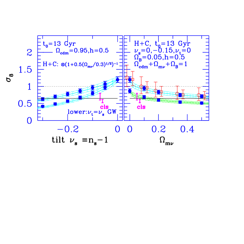
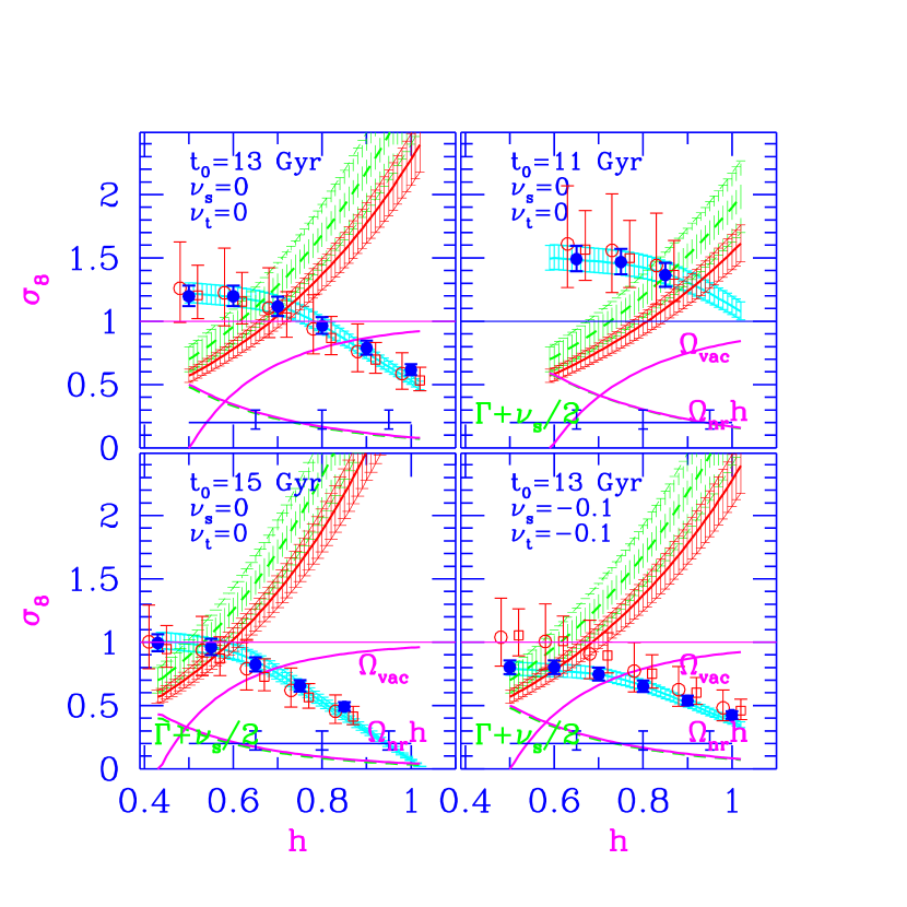
Figure 6: This illustrates the accuracy and utility of the fitting formula for $\sigma_{8}$ for a variety of inflation-inspired cosmological models. The lower figure also includes large scale structure and cluster abundance constraints. The symbols are defined in the text.

Although Fig. 6 gives a visual impression of which models are preferred, this can be put on a more quantitative basis. Fig. 6 shows $\sigma_{8}$ is a sensitive function of $n_{s}$: for CDM models with $\Omega_{nr}=1$, it is far too high at $1.2$ for $n_{s}$=1, but too low by $n_{s}\approx 0.76$ with the “standard” gravity wave contribution ($\nu_{t}=\nu_{s}$) or by $n_{s}\approx 0.60$ if there is no tensor mode contribution. However, the shape constraint wants lower $n_{s}$. In [13], we marginalize likelihood functions determined with the COBE data (and smaller angle data) using a prior probability requiring that $\Gamma+\nu_{s}/2$ be $0.22\pm 0.08$ and $\sigma_{8}\Omega_{nr}^{0.56}$ be $0.65^{+0.15}_{-0.08}$ in order to condense the tendencies evident in Fig. 6 into single numbers with error bars. Threading the “eye of the needle” this way is so exacting that the error bars are too small to take too seriously. Sample numbers using only the 4-year dmr data and these priors for the 13 Gyr case are: $n_{s}=0.76^{+.03}_{-.03}$ for ${\rm h}=0.5$ with gravity waves, $0.61^{+.04}_{-.04}$ without, i.e., much tilt; for ${\rm h}=0.7$ and $\Omega_{vac}=0.66$, we get $0.99^{+.03}_{-.02}$ with and $0.94^{+.04}_{-.04}$ without, i.e., little tilt; and when Hubble parameters in the range from 0.5 to 1 are marginalized over, the preferred index is $n_{s}=0.99^{+.06}_{-.04}$ with gravity waves, $0.95^{+.09}_{-.10}$ without, i.e., again little tilt. Combining sp94 and sk93+94 with dmr data does not change the values nor the error bars by much (it flattens a bit). When all smaller angle data is used plus LSS and dmr4 data, and $H_{0}$ is marginalized, $n_{s}=0.96\pm 0.03$ is obtained, again not very different from the LSS + dmr4 only result. In both cases, a nonzero $\Omega_{vac}$ is preferred.

For the decaying neutrino model with $n_{s}=1$ to have $\sigma_{8}>0.5$ we need $\Gamma>0.22$, i.e., $m_{\nu}\tau_{d}<14~{}{\rm keV~{}yr}$. The hot/cold hybrid model formula in eq. (12) is for one massive neutrino species. As Fig. 6 shows, an $n_{s}$=1 ${\rm h}$=0.5 hot/cold hybrid model with $\Omega_{\nu}<0.3$ would have $\sigma_{8}>0.8$; however, even with a modest tilt to $n_{s}=0.95$ this can drop to 0.7 for $\Omega_{\nu}=0.25$. (See also ref. [83].) That is, little tilt is required, in contrast to the CDM case.

It is also evident from Fig. 6 that the cluster data in combination with the dmr data stops ${\rm h}$ from becoming too high for a fixed age, but also would prefer a nonzero $\Lambda$ value, with $H_{0}\sim 60-70$ for 13 Gyr, and $H_{0}\sim 50-60$ for 15 Gyr. When the tilt is allowed to vary as well, the preferred values lower to very near 50 and 43, respectively, i.e., with little $\Omega_{vac}$: $h<0.70$ at $2\sigma$ with gravity waves, $h<0.56$ with no gravity waves for 13 Gyr; $h<0.56$ at $2\sigma$ with gravity waves for 15 Gyr. For the hot/cold models, the values near 50 and 43 are preferred even more, even with very little tilt.

For open CDM models, the COBE-determined $\sigma_{8}$ goes down with decreasing $\Omega$ (and increasing ${\rm h}$). These models are not so attractive because $\Omega$ drops so precipitously with increasing ${\rm h}$ for fixed age (e.g., for 13 Gyr and $H_{0}=70$, $\Omega_{tot}$=0.055). Equation (12) has not been modified to treat open models (see e.g., [94]).

Texture and string models require a low $\sigma_{8}$, $<0.5$. At this stage, it is still unclear how much of a problem this is since non-Gaussian effects can modify the cluster distribution, partly compensating for the low $\sigma_{8}$.

Going to higher $k$-bands, COBE-normalized spectra imply values for the “the redshift of galaxy formation”, of quasar formation, and the amount of gas in damped Lyman alpha systems etc. and this also significantly restricts the parameter space. However, it is more dependent on the role gasdynamics may play in defining the objects.

If we are so bold as to assume that we now know the shape of the density power spectrum over the large scale structure band, and the amplitude of the power spectrum on cluster-scales, then, in conjunction with the COBE anisotropy level, the range of inflation and dark matter models is considerably restricted. Whether the solution will be a simple variant on the CDM+inflation theme [92], involving slight tilt (or more radical broken scale invariance), stable ev-mass neutrinos, decaying ($>$kev)-neutrinos, vacuum energy, low $H_{0}$, high baryon fraction, mean curvature, or some combination, is still open, but can be decided as the observations tighten, and, in particular, as the noise in the ${\cal C}_{\ell}$ figure subsides, revealing the details of the Doppler peaks, a very happy future for those of us who wish to peer into the mechanism by which structure was generated in the Universe.

ACKNOWLEDGMENTS: The CMB field has seen an explosion of papers since the COBE discovery. The reference list given here is truncated. For a more complete list see [1, 2]. Thanks to my collaborators Andrew Jaffe, Yoram Lithwick, and Tarun Souradeep for permission to quote some of our unpublished work. Support from NSERC and a Canadian Institute for Advanced Research Fellowship is gratefully acknowledged.

References

- [1] Bond, J.R. 1996, Theory and Observations of the Cosmic Background Radiation,in “Cosmology and Large Scale Structure”, pp. 469-674, Les Houches Session LX, August 1993, ed. R. Schaeffer, Elsevier Science Press.
- [2] White, M., Scott, D. & Silk, J. 1994, Ann. Rev. Astron. Ap. 32, 319
- [3] Bond, J.R., Crittenden, J.R., Davis, R.L., Efstathiou, G. & Steinhardt, P.J., 1994, Phys. Rev. Lett. 72, 13
- [4] Knox, L. 1995, Phys. Rev. D 52, 4307.
- [5] Jungman, G., Kamionkowski, M., Kosowsky, A. & Spergel, D.N. 1996, Phys. Rev. Lett. 76, 1007.
- [6] Bennett, C. et al. 1996, MAP experiment home page, http://map.gsfc.nasa.gov
- [7] Janssen, M.A. et al. 1997, Ap. J. , in press, astro-ph/9602009.
- [8] Bersanelli, M. et al. 1996, COBRA/SAMBA, The Phase A Study for an ESA M3 Mission, preprint.
- [9] Bond, J.R., Efstathiou, G. & Tegmark, M. 1997, astro-ph/9702100.
- [10] Zaldarriaga, M., Spergel, D. & Seljak, U. 1997, astro-ph/9702157.
- [11] Fixsen, D.J. et al. 1996, Ap. J. 473; Mather, J.C. et al. 1994, Ap. J. Lett. 420, 439.
- [12] Bond, J.R. 1995, Phys. Rev. Lett. 74, 4369
- [13] Bond, J.R. & Jaffe, A., 1996, Cosmic Parameter estimation combining sub-degree CMB experiments with COBE. Proc. XXXI Rencontre de Moriond, ed. F. Bouchet, Edition Frontieres.
- [14] Tegmark, M. & Efstathiou, G. 1996, M.N.R.A.S. 281, 1297
- [15] Gautier, T.N. et al. 1992, AJ 103, 1313.
- [16] Kogut, A. et al. 1996, Ap. J. 460, 1.
- [17] Reach, W. et al. 1995, Ap. J. 451, 188.
- [18] Puget, J.-L. et al. 1996, Astron. Ap. 308, L5.
- [19] Walker, T.P., Steigman, G., Schramm, D.N., Olive, K.A. & Kang, H.S. 1991, Ap. J. 376, 51; Smith, M.S., Kawano, L.H. & Malaney, R.A. 1993, Ap. J. Supp. 85, 219
- [20] Gush, H.P., Halpern, M. & Wishnow, E. 1990, Phys.Rev. Lett. 65, 537
- [21] Zeldovich, Ya.B. & Sunyaev, R.A. 1969, Ap. Space Sci. 4, 301
- [22] Bartlett, J. & Stebbins, A. 1991, Ap. J. 371, 8
- [23] Bond, J.R. & Myers, S. 1996, Ap. J. Supp. 103, 63.
- [24] Bond, J.R., Carr, B.J. & Hogan, C.J. 1986, Ap. J. 306, 428; 1991, Ap. J. 367, 420; Bond, J.R. & Myers, S. 1993, in: M. Shull & H. Thronson, eds., The Evolution of Galaxies and their Environment, Proceedings of the Third Teton Summer School, NASA Conference Publication 3190, p. 21.
- [25] Hauser, M.G. 1995, in Unveiling the Cosmic Infrared Background, ed. E. Dwek, AIP Conference Proceedings, (AIP, New York); 1995, IAU Symposium 168, Examining the Big Bang and Diffuse Background Radiations, ed. M. Kafatos & Y. Kondo (Kluwer, Dordrecht).
- [26] Bertschinger, E., Bode, P., Bond, J.R., Coulson, D., Crittenden, R., Dodelson, S., Efstathiou, G., Gorski, K., Hu, W., Knox, L., Lithwick, Y., Scott, D., Seljak, U., Stebbins, A., Steinhardt, P., Stompor, R., Souradeep, T., Sugiyama, N., Turok, N., Vittorio, N., White, M., Zaldarriaga, M. 1995, ITP workshop on Cosmic Radiation Backgrounds and the Formation of Galaxies, Santa Barbara
- [27] Salopek, D.S., Bond, J.R. & Bardeen, J.M. 1989, Phys. Rev. D 40, 1753
- [28] Kofman, L. & Starobinsky, A.A. 1985, Sov. Astron. Lett. 11, 271
- [29] Ratra, B. & Peebles, P.J.E. 1994, Ap. J. Lett. 432, L5; Phys. Rev. D 50, 5232, Phys. Rev. D , in press (PUPT-1444)
- [30] Kamionkowski, M., Ratra, B., Spergel, D.N. & Sugiyama, N. 1994, Ap. J. Lett. 434, L1
- [31] Bond, J.R. & Souradeep, T. 1997, preprint.
- [32] Efstathiou, G. & Bond, J.R. 1986, M.N.R.A.S. 218, 103
- [33] Efstathiou, G. & Bond, J.R. 1987, M.N.R.A.S. 227, 33P
- [34] Allen, B., Caldwell, R.R., Shellard, E.P.S., Stebbins, A. & Veeraraghavan, S. 1996, Phys. Rev. Lett. 77, 3061.
- [35] Bennett, D.P. & Rhie, S.H. 1993, Ap. J. Lett. 406, 7; Pen, Ue-Li, Spergel, D.N. & Turok, N. 1994, Phys. Rev. D 49, 692.
- [36] Coulson, D.,Ferreira, P., Graham, P. & Turok, N. 1994, Nature 368, 27.
- [37] Crittenden, R. & Turok, N. 1995, Phys. Rev. Lett. 75, 2642.
- [38] Allen, B., Caldwell, R.R., Dodelson, S., Knox, L., Shellard, E.P.S. & Stebbins, A. 1997, preprint, astro-ph/9704160.
- [39] Pen, Ue-Li, Seljak,U. & Turok, N. 1997, preprint, astro-ph/9704165.
- [40] Bond, J.R. 1995, Astrophys. Lett. & Comm. 32, 63.
- [41] Ma, C.-P. & Bertschinger, E. 1995, Ap. J. 455, 7.
- [42] Dodelson, S., Gates, E. & Stebbins, A. 1996 Ap. J. 467, 10.
- [43] Bond, J.R. & Lithwick, Y. 1995, unpublished (see [1]).
- [44] Bond, J.R. & Efstathiou, G. 1984, Ap. J. Lett. 285, L45.
- [45] Vishniac, E.T. 1987, Ap. J. 322, 597.
- [46] Seljak, U. 1994, Ap. J. Lett. , in press
- [47] Kaiser, N. 1992, Ap. J. 388, 272; 1992, in New Insights of the Universe, Proc. Valencia Summer School, Sept. 1991
- [48] Smoot, G.F., et al. 1992 Ap. J. Lett. 396, L1; Bennett, C. et al. 1994, Ap. J. 436, 423
- [49] Bennett, C. et al. 1996, Ap. J. Lett. 464, 1; and 4-year DMR references therein. [dmr]
- [50] A. Kogut et al. 1996, Ap. J. Lett. 464, 5.
- [51] Hinshaw, G. et al. 1996, Ap. J. Lett. 464, 17.
- [52] Ganga, K., Cheng, E., Meyer, S. & Page, L. 1993, Ap. J. Lett. 410, L57; Ganga, K., Page, L., Cheng E. & Meyer, S. 1994, Ap. J. Lett. 432, L15 [firs]
- [53] Gutteriez de la Cruz, S.M. et al. 1995, Ap. J. 442, 10; Hancock, S. et al. 1993, Nature 367, 333; Watson R. et al. 1992, Nature 357 660 [ten]
- [54] Gaier, T. et al. 1992, Ap. J. Lett. 398 L1; Schuster, J., et al. 1993, Ap. J. Lett. 412, L47 [sp91]
- [55] Bond, J. R. 1994, Cosmic Structure Formation & the Background Radiation, in ”Proceedings of the IUCAA Dedication Ceremonies,” Pune, India, Dec. 28-30, 1992, ed. T. Padmanabhan, Wiley
- [56] Gundersen, J. et al. 1994, Ap. J. Lett. , 443, L57 [sp94].
- [57] Wollack, E.J. et al. 1993, Ap. J. Lett. 419, L49 [sk93]
- [58] Netterfield, C.B., Jarosik, N., Page, L. & Wilkinson, D. 1995, Ap. J. Lett. 455, L69. [sk94]
- [59] Netterfield, C.B., Devlin, M.J., Jurosik, N., Page, L. & Wollack, E.J. 1997, Ap. J. 474, 47 [sk95]
- [60] Dragovan, M. et al. 1994, Ap. J. Lett. 427, L67 [py]
- [61] de Bernardis, P. et al. 1994, Ap. J. Lett. 422, L33 [ar]
- [62] Clapp, A. et al. 1994, Devlin, M. et al. 1994, Ap. J. 430, 1 [max4, M4]; Meinhold, P., et al. 1993, Ap. J. Lett. 409, L1; Gunderson, J., et al. 1993, Ap. J. Lett. 413, L1 [MAX3, M3]
- [63] Tanaka, S. et al. 1996, Ap. J. Lett. 468, 81 [max5, M5].
- [64] Cheng, E.S. et al. 1993, Ap. J. Lett. 420, L37 [msam2 (g2),msam3 (g3)]
- [65] Scott, P.F. et al. 1996, Ap. J. Lett. 461, 1 [cat]
- [66] Readhead, A.C.S. et al. 1989, Ap. J. Lett. 346, 556 [ov7]
- [67] Meinhold, P. & Lubin, P. 1991, Ap. J. Lett. 370, 11 [sp89]
- [68] Tucker, G.S. et al. 1993, Ap. J. Lett. 419, L45 [wd2, wd1]
- [69] Chibisov, G. & Mukhanov, V.F. 1982, M.N.R.A.S. 200, 535; Mukhanov, V.F., Feldman, H.A. & Brandenberger, R.H. 1992, Phys. Rep. 215, 203; Lyth, D.H. 1985, Phys. Rev. D 31, 1792
- [70] Bardeen, J. M. 1980, Phys. Rev. D 22, 1882
- [71] Lyth, D.H. & Stewart, E.D. 1992, Phys. Lett. 274B, 168.
- [72] Salopek, D.S. & Bond, J.R. 1990, Phys. Rev. D 42, 3936; 1991, Phys. Rev. D 43, 1005
- [73] Bardeen, J., Steinhardt, P. J. & Turner, M. S. 1983, Phys. Rev. D 28, 679
- [74] Bardeen, J.M., Bond, J.R., Kaiser, N. & Szalay, A.S. 1986, Ap. J. 304, 15
- [75] Starobinsky, A.A. 1979, Pis’ma Zh. Eksp. Teor. Fiz. 30, 719; 1985, Sov. Astron. Lett. 11, 133.
- [76] Abbott, L.F. & Wise, M. 1984, Nucl. Phys. B 244, 541.
- [77] Crittenden, R., Bond., J.R., Davis., R.L., Efstathiou, G. & Steinhardt, P.J., 1993, Phys. Rev. Lett. 71, 324; and post-COBE references therein.
- [78] Bond, J.R. 1994, Testing Inflation with the Cosmic Background Radiation, in Relativistic Cosmology, Proc. 8th Nishinomiya-Yukawa Memorial Symposium, ed. M. Sasaki, Academic Press, astro-ph/9406075
- [79] Bond, J.R., Efstathiou, G., Lubin P.M. & Meinhold, P. 1991, Phys. Rev. Lett. 66, 2179.
- [80] Peacock, J.A. & Dodds, S.J. 1994, M.N.R.A.S. 267, 1020
- [81] Sugiyama, N. 1995, Astrophys. J. Supp. 100, 281.
- [82] Efstathiou, G., Bond, J.R. & White, S.D.M. 1992, M.N.R.A.S. 258, 1P
- [83] Pogosyan, D.Yu. & Starobinsky, A.A. 1993, M.N.R.A.S. 265, 507; 1995 Ap. J. 447, 465.
- [84] Kofman, L., Gnedin, N. & Bahcall, N. 1993, Ap. J. 413, 1.
- [85] Adams, F.C., Bond, J.R., Freese, K., Frieman, J.A. & Olinto, A.V. 1993, Phys. Rev. D , 47, 426
- [86] Chaboyer, B. et al. 1997, preprint, astro-ph/9706128.
- [87] White, S.D.M., Efstathiou, G., & Frenk, C.S., 1995, M.N.R.A.S. 292, 371
- [88] Eke, V.R., Cole, S. & Frenk, C.S. 1996, M.N.R.A.S. 282, 263
- [89] Strauss, M. & Willick, J. 1995, Phys. Rep. 261, 271
- [90] Zaroubi, S. et al. 1996, preprint, astro-ph/9603068
- [91] Kolatt, T. & Dekel, A. 1997, Ap. J. 479, 592.
- [92] Bardeen, J.M., Bond, J.R. & Efstathiou, G. 1987, Ap. J. 321, 28
- [93] Bond, J.R. & Efstathiou, G. 1991, Phys. Lett. B 379, 440
- [94] Gorski, K.M., Ratra, B., Sugiyama, N. & Banday, A.J. 1995, Ap. J. Lett. 444.