A Simultaneous Spectral Invariant Analysis of the GRB Count Distribution and Time Dilation.

Abstract

The analysis of the BATSE’s count distribution within cosmological models suffers from observational uncertainties due to the variability of the bursts’ spectra: when BATSE observes bursts from different redshifts at a fixed energy band it detects photons from different energy bands at the source. This adds a spectral dependence to the count distribution $N(C)$. Similarly variation of the duration as a function of energy [1] at the source complicates the time dilation analysis. It has even been suggested that these methods lead to inconsistent estimates of the redshift from which the bursts are observed[2]. Clearly it would be best to combine the estimates and to perform a joint analysis of the strength and the duration of the bursts. But for this we have to eliminate first the spectral dependence problem.

We describe here a new statistical formalism that performs the required “blue shifting” of the count number and the burst duration in a statistical manner. This formalism allows us to perform a combined best fit (maximal likelihood) to the count distribution, $N(C)$, and the duration distribution simultaneously. The outcome of this analysis is a single best fit value for the redshift of the observed bursts.

Introduction

When BATSE observes bursts from different red-shifts at a fixed energy band it detects photons from different energy bands at the source. This spectral dependence complicates the interpretation of the peak-flux and time-dilation distributions. So far several attempts have been made to overcome this problem by modeling the spectral shape of the bursts. We suggest here a different method which is based on the availability of multi channel data in different energy bands. The basic idea beyond our scheme is that we “view” all bursts at the same intrinsic energy band independently of their red-shift by by scanning over the different channels until we find the most likely red-shift and using this value to “blue-shift” back the observed spectrum to the initial spectrum at the source. Now we look at the same energy band at the source for all bursts, avoiding the issue of the spectral shape.

Standard candle sources.

Consider first a population of standard candle sources that have a fixed luminosity, $L$, at a given energy band centered around an energy $E$. For each burst we have a set of measured peak fluxes $C_{i}(E_{i})$ at different energy bands. We determine the red-shift of a particular burst by solving the equation:

$$L=L(z)=C({E\over 1+z})d_{L}^{2}(z)(1+z)^{-2}\ ,$$ (1)

where $d_{L}$ is the luminosity distance and $C({E\over 1+z})$ is the observed peak-flux at the energy $E\over 1+z$.

One may wonder whether there will be multiple solutions to this equation. The answer is surprisingly no, provided that the spectrum is softer than $N(E)dE\propto E^{-1}dE$. As an example we consider a simulated source with a spectral shape: $N(E)dE\propto E^{-\alpha}dE$. Figure 1 shows the luminosity as calculated by this method for simulated sources with $\alpha=2.5$ (upper sheet) and $\alpha=1$ (lower sheet) in an $\Omega=1$ cosmology. The only $z$ which solves the luminosity equation is the actual redshift.

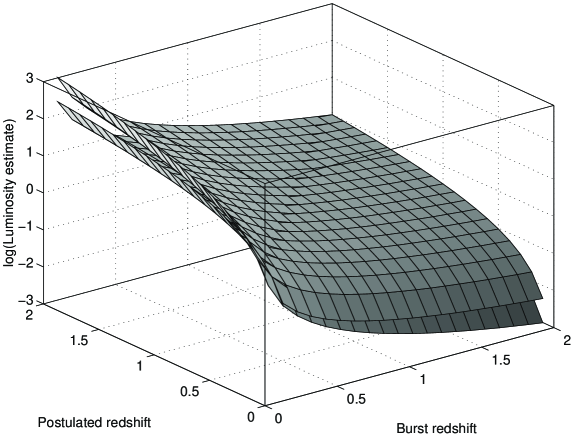
FIG. 1.: The “blue-shifted” luminosity of an observed burst with an intrinsic luminosity $L=1$, with power-law parameter $\alpha=2.5$ (upper sheet) and $\alpha=1$ (lower sheet) in an $\Omega=1$ cosmology, for different assumed $z$ values. The correct luminosity $L=1$ is obtained only when the chosen $z$ is the same as the real one.

Once we obtain the red-shift for each burst we proceed to compare the red-shift distribution with the one predicted by a different cosmological models. This is done, for example, by using the maximum likelihood method. We check whether the method is consistent by repeating the whole process for different energy channels (at the source). If there is no noise the different channels should give the same red-shift distribution.

Sources with variable luminosity.

In reality we don’t have standard candle sources. Current estimates suggest that the GRB luminosity function is quite narrow (with variation of peak flux of no more then one order of magnitude) but it is unlikely that it is a delta function. Thus, the luminosity of a burst is not known a priori, and the redshift can not be deduced uniquely from the peak flux. However, this method can be used in a statistical manner even when faced with this uncertainty.

We assume that the bursts have a known luminosity function $\phi(L)$ at a standard energy band at the source. In fact all that we need to assume is that $\phi(L)$ has a given functional shape characterized by a few parameters which will be determined by the analysis. As in the standard candle case we blue-shift the peak flux in each of the energy channels by a suitable factor $(1+z)$ to our canonical energy at the source and we calculate the corresponding luminosity: $L(z)$, using equation 1. We then estimate the likelihood that the burst is at redshift $z$i as:

$$h(z)=\phi(L(z)){dL\over dz}\equiv\tilde{\phi}(L(z))\ .$$ (2)

For standard candles $\phi(L)=\delta(L-L_{0})$ and $h(z)=\delta(z-z_{0}))$. Figure 2 depicts the spread in $z$ due to a power-law luminosity distribution:

$$\phi(L)=\left\{{\matrix{{\left({L\over L_{0}}\right)}^{3}&L<L_{0}\cr{\left({L\over L_{0}}\right)}^{-3}&L>L_{0}\cr}}\right.$$ (3)

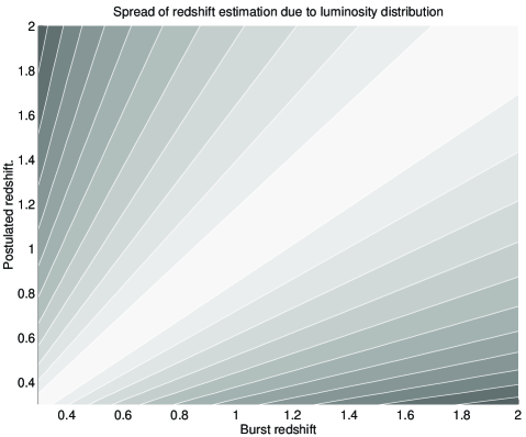
FIG. 2.: Figure 2: Likelihood of a burst from redshift z to be detected as a nominal burst from a postulated redshift. Standard candle sources would make the graph non zero only on the main diagonal. The spread is due to a power-law luminosity distribution given by Eq. 3. The lines represents $33\%$, $10\%$, $3.3\%$… likelihood.

A given cosmological model, with a given evolution model (that is number density of bursts per co-moving as a function of cosmological time) determines $n(z)dz$, the expected number of bursts from a $dz$ interval centered around $z$, per observer unit time. With a given luminosity function at a fixed energy band at the source we calculate now the likelihood of a burst, given the set of data $C_{i}(E_{i})$:

$$\matrix{P(C_{1\ldots n})=\int n(z)h(z)dz\cr=\sum_{i}\tilde{\phi}\left[{C_{i}({E\over 1+z_{i}})d_{L}(z_{i})^{2}(1+z_{i})^{-2}}\right]n(z_{i})\ .}$$ (4)

Once we have this estimate for the likelihood of all bursts we proceed to write the likelihood function of the whole set of data. Then we use the maximal likelihood method to estimate the most likely cosmological parameters and the luminosity function parameters.

It is apparent that as the luminosity distribution widens, the constrain on the redshift weakens, and the information about cosmology is vaguer. The difference between reasonable spectrums is not large. For example to confuse a redshift $z=0.5$ bursts and a redshift $z=1$ with $\alpha=2$ requires a luminosity factor of $4.5$ while $\alpha=1$ requires a luminosity factor of $3.4$. Naturally, as the amount of data increases, the confidence in the determination of $z$ increases. Once more, self consistency requires that similar results are obtained when using different energy channels.

A joint analysis of time-dilation.

The time-dilation analysis should be combined with the peak-flux estimate. The combined analysis provide a self consistent method which estimates the red-shift of each burst using both sets of data. This should be more accurate than the standard analysis [3] ,[4],[5] in which the bursts are grouped into large groups of bright, dim and dimmest bursts.

Using the spectral invariant method we view all bursts in the same intrinsic energy, and in this way we eliminate the energy dependence of the bursts’ duration. Now we would like to combine information about the duration of a burst in the different energy channels, $\delta t_{i}(E_{i})$ (this could be $\Delta t_{50}$ or alternatively the autocorrelation characteristic time) with the set of peak-fluxes $C_{i}(E_{i})$. We estimate the likelihood of the burst as:

$$\matrix{P(C_{1\ldots n},\delta t_{1\ldots n})=\int n(z)h(z)\Psi\left[{{\delta t({E\over 1+z})\over 1+z},E}\right]dz=\cr\sum_{i}n(z_{i})\tilde{\phi}\left[{C({E\over 1+z_{i}})d_{L}(z_{i})^{2}(1+z_{i})^{-2})}\right]\Psi\left[{{\delta t_{i}({E\over 1+z_{i}})\over 1+z_{i}},E}\right]}$$ (5)

Where $\Psi(t,E)$ is the intrinsic energy dependent duration distribution function. Using the maximum likelihood method we can now estimate the best-fit parameters of the luminosity function, $\tilde{\phi}$, the duration distribution, $\Psi(t,E)$, and the maximal redshift from which the bursts are observed.

Discussion

The spectrum invariant method is the only way to have a complete usage of all the information available in the multi-spectral channel detectors in situations in which the spectra is being red-shifted differently from burst to burst. It also uses the time-dilation and the peak-luminosity in a way that more than just brings a consistent answer, it uses the whole data to enlarge the statistical confidence of the results. A luminosity distribution influences considerably the confidence the red-shift determination of a single burst origin. However, it has a minor influence when using a large number of bursts. Similarly the duration distribution makes it impossible to determine the red-shift of a single burst, however one can determine the parameters of the duration distribution and find whether the red-shift data determined from the time dilation analysis is consistent with the one determined from the peak-flux distribution.

REFERENCES

- [1] Fenimore, E. E., et al, 1995, ApJL, 448, 101L
- [2] Fenimore, E. E., and Bloom, J. S., 1995, ApJ, 453, 25.
- [3] Norris, J. P., et al, 1994, ApJ. 424, 540.
- [4] Band, D. L., 1994, ApJL.
- [5] Wijers, R. A. M. J., and Paczyński, B., 1994, ApJL, 437, 107L.