Large-Scale Structure at $z\sim 2.5$

Abstract

We have made a statistically complete, unbiased survey of C iv systems toward a region of high QSO density near the South Galactic Pole using 25 lines of sight spanning $1.5<z<2.8$. Such a survey makes an excellent probe of large-scale structure at early epochs. We find evidence for structure on the $15-35h^{-1}$ proper Mpc scale ($H_{0}\equiv 100$ km s^-1 Mpc${-1}$) as determined by the two point C iv-C iv absorber correlation function, and reject the null hypothesis that C iv systems are distributed randomly on such scales at the $\sim 3.5\sigma$ level. The structure likely reflects the distance between two groups of absorbers subtending $\sim~{}13\times 5\times 21h^{-3}$ and $\sim 7\times 1\times 15h^{-3}$ Mpc³ at $z\sim 2.3$ and $z\sim 2.5$ respectively. There is also a marginal trend for the association of high rest equivalent width C iv absorbers and QSOs at similar redshifts but along different lines of sight. The total number of C iv systems detected is consistent with that which would be expected based on a survey using many widely separated lines of sight. Using the same data, we also find 11 Mg ii absorbers in a complete survey toward 24 lines of sight; there is no evidence for Mg ii-Mg ii or Mg ii-QSO clustering, though the sample size is likely still small to detect such structure if it exists.

1 Introduction

QSO absorption lines provide the means to study large-scale structure far beyond the $z\mathrel{\hbox to0.0pt{\lower 3.0pt\hbox{$\mathchar 536\relax$}\hss}\raise 2.0pt\hbox{$\mathchar 316\relax$}}0.5$ limits of current galaxy surveys. They are a natural extension of pencil beam galaxy surveys (Broadhurst et al. 1990) which claim to find structure at $z<0.5$, and which have sparked interest in “foam” models for large scale structure (e.g. Icke & van de Weygaert 1987, Coles 1990, van de Weygaert 1991, SubbaRao & Szalay 1992). However, regions of sufficient surface density of bright, high-$z$ QSOs which can provide enough systems to outline structure in three dimensions at high redshift and to discriminate between some of the various models (Kaiser & Peacock 1991) are rare. In this paper we investigate the region with the highest known surface density of bright, high redshift QSOs, mapping structure at $z>1.5$ using C iv absorption systems.

Earlier work of this type explored the common C iv absorption in the vicinity of Tol 1037-2703 and Tol 1038-2712 (Jakobsen & Perryman 1992). The 17 CIV systems at $1.8\mathrel{\hbox to0.0pt{\lower 3.0pt\hbox{$\mathchar 536\relax$}\hss}\raise 2.0pt\hbox{$\mathchar 316\relax$}}z\mathrel{\hbox to0.0pt{\lower 3.0pt\hbox{$\mathchar 536\relax$}\hss}\raise 2.0pt\hbox{$\mathchar 316\relax$}}2.2$ extend over nearly a degree, outlining a sheet-like structure $5-10\times 40-50h^{-2}$Mpc² seen nearly edge-on ($H_{0}=100h$ km s^-1 Mpc^-1, $q_{0}=0.5$ and $\Lambda=0$ are assumed throughout). A similar study was made toward PKS 0237-233. Foltz et al. (1993) selected it a priori  on the evidence of a C iv cluster (Heisler, Hogan & White 1989) found in a survey spanning many widely distributed lines of sight by Sargent, Boksenberg, & Steidel (1988, hereafter SBS). There appears to be a spatial overdensity of CIV systems over $1.58\mathrel{\hbox to0.0pt{\lower 3.0pt\hbox{$\mathchar 536\relax$}\hss}\raise 2.0pt\hbox{$\mathchar 316\relax$}}z\mathrel{\hbox to0.0pt{\lower 3.0pt\hbox{$\mathchar 536\relax$}\hss}\raise 2.0pt\hbox{$\mathchar 316\relax$}}1.67$ along the lines of sight to 6 high $z$ QSOs with $12-16$ C iv systems spanning up to $65h^{-1}$Mpc, but most of the absorption is seen only toward two QSOs.

The new QSO field which forms the basis for the present work was found by Hazard et al. (1995) from an objective prism survey in the South Galactic Cap. There are 25 confirmed QSOs within a $\sim 1$ deg² region having redshifts $1.5\mathrel{\hbox to0.0pt{\lower 3.0pt\hbox{$\mathchar 536\relax$}\hss}\raise 2.0pt\hbox{$\mathchar 316\relax$}}z\mathrel{\hbox to0.0pt{\lower 3.0pt\hbox{$\mathchar 536\relax$}\hss}\raise 2.0pt\hbox{$\mathchar 316\relax$}}3.4$. These QSOs are more closely spaced, brighter and at higher redshift than the QSO fields studied by Jakobsen & Perryman (1992) and Foltz et al. (1993). Therefore, it is possible to search a relatively longer baseline for C iv systems at higher spectral and spatial resolution than in previous studies. The results are then compared with general C iv properties determined from SBS and Steidel (1990). Only two of the QSOs in this SGP region have previously been surveyed for C iv absorption (Steidel 1990). A study of this region will indicate whether or not such C iv absorber associations as those in the Tol $1037-2703$/$1038-2712$ and PKS $0237-233$ fields are common. It is also useful for studying the distribution of Ly$\alpha$ forest lines along closely spaced lines of sight. We present results for a spectroscopic survey of these QSOs to search for C iv absorbers as indications of large scale structure. The observations are described in § 2. The absorption system selection and descriptions of individual spectra are in § 3. The results of various cross-correlations are described and discussed in § 4, with conclusions in § 5.

2 Observations and Reductions

The observations were made on the CTIO 4m telescope over two observing sessions covering 1992 September 25-27 and 1993 October 14-17 respectively, under conditions of variable transparency with $1.2-3.0$ arcsec seeing. The data were taken using the Argus multifiber spectrograph in conjunction with a Reticon CCD. Two 632 line/mm gratings were used to permit data coverage spanning 1120 Å in a single exposure, using three different bandpasses (3835–4954, 4594–5713, 4810–5926 Å). Nine separate Argus pointings were used, all centered around RA 00^h 42^m, dec $-26^{\circ}40^{\prime}$. This permitted observations of all previously confirmed QSOs with $z>1.5$ in the Hazard et al. field to be observed in the unvignetted 48 arcmin diameter Argus field of view. The remaining fibers were used to observe additional QSOs and QSO candidates from the Hazard et al. list as well as a number of faint QSOs with $z\mathrel{\hbox to0.0pt{\lower 3.0pt\hbox{$\mathchar 536\relax$}\hss}\raise 2.0pt\hbox{$\mathchar 318\relax$}}3$ from the deep multi-color surveys of Warren, Hewett, & Osmer (1991). Coordinates for the fiber positioning were measured with the Automated Plate Measuring machine at Cambridge, England (Kibblewhite et al. 1984). The data were extracted optimally using a routine adapted from that used in Rauch et al. (1992). The variance for each pixel was determined based on photon counting statistics from the object, sky and readout noise. Final spectra for each object were formed by adding the sky-subtracted, extinction corrected, flux calibrated spectra from each frame, using inverse variance weighting. The resolution is $\sim 2$Å. In all, spectra were obtained for a total of 26 QSOs. Their positions, the best estimate that we have for the emission line redshifts and the relevant exposure times are given in Table 1. The surface distribution of the QSOs is illustrated in Figure 1, while the individual spectra are presented in Figure 2.

3 Spectra and Absorption Systems

3.1 Individual Spectra

Although the primary purpose of this study is to study large-scale structure using C iv absorption systems, we note a few other items of interest concerning the spectra. Overall, we do not detect any candidate damped Ly$\alpha$ absorbers. We consider spectra ranges for the 11 QSOs where the signal-to-noise ratio is sufficient for a 4$\sigma$ detection of a Ly$\alpha$ line of rest equivalent width $W_{0}=5.0$Å, up to 3000 km s^-1 from Ly$\alpha$ emission. Using the statistics of Lanzetta et al. (1991), with redshift density $d{\cal N}/dz=N_{0}(1+z)^{\gamma}$, $N_{0}=0.16\pm 0.03$, $\gamma=0.3\pm 1.4$, we expect 0.2, 1.3, 7.8 damped Ly$\alpha$ systems for $N_{0}=0.16$ and $\gamma=-1.1,0.3,1.7$. We conclude that the region is not anomalously under-dense in damped Ly$\alpha$ systems. We find one obvious BAL in the sample of 26 QSOs, consistent with a frequency of occurrence of $\sim 10$% ; these objects are worthy of further study with greater resolution and spectral coverage. We call attention to the following spectra.

Q$0041-2658$ ($z_{em}=2.457$): There is a complex absorption feature to the blue of C iv $\lambda\lambda 1548,1550$ which corresponds in extent and shape to an absorption feature at the corresponding position of N v $\lambda\lambda 1238,1242$ as well as Ly$\alpha$ absorption. However, the line ratio at 4255–4275 Å (near where associated N v $\lambda\lambda 1238,1242$ would be expected) is consistent with that of Mg ii $\lambda\lambda 2796,2803$. Also, no Si iv $\lambda\lambda 1393,1402$ nor Si ii $\lambda 1260$ are found at $z=2.4264,2.4383$. The automated search procedure may not give consistently good results over such regions, and so only the general troughs are noted.

Q$0042-2656$ ($z_{em}=3.33$): There is a high equivalent width Ly$\alpha$ line at $z=3.3303$ (rest equivalent width $W_{0}=1.65$Å) which may be associated with the QSO. However, a search for metals at the same redshift using Morton’s (1991) line list only reveals a match for Si ii $\lambda 1304$. This would be coincident with C iv $\lambda 1548$ at $z=2.6489$, the presence of which is strongly supported by Ly$\alpha$ absorption with rest equivalent width $W_{0}=1.39$Å.

Q$0042-2714$ ($z_{em}=2.36$): There is strong Ly$\alpha$ absorption just blueward of Ly$\alpha$ emission, which may indicate strong associated absorption. Unfortunately, wavelength coverage is insufficient to confirm this with C iv $\lambda 1550$.

Q$0043-2647$ ($z_{em}=2.12$): This is an extreme example of the BAL phenomenon. We have excluded the spectrum blueward of 4800 Å from our analysis, with the region from $4250-4800$ Å dominated by C iv and Si iv features, with additional BAL absorption further to the blue. We have also not attempted to deblend any of the lines in the region $4580-4800$ Å.

Absorption Line Measurements

The main objective of this work is an investigation of clustering using intervening C iv absorbers. However, because our sample contains so many high redshift QSOs, it also provides much valuable data of Ly$\alpha$ forest absorption systems. Therefore, we have not confined our analysis to the red of Ly$\alpha$ but when possible have also produced lists of Ly$\alpha$ forest lines. The presence of high equivalent width Ly$\alpha$ forest lines is also useful to check independently the validity of suspected metal absorption systems. Absorption lines were searched for with automated software using the statistically based procedure described in Young et al. (1979). All features significant at the 4$\sigma$ level were noted. For metal line doublets, features with both components at the $\geq 3\sigma$ significance are used, subject to their being consistent with laboratory wavelength and equivalent width ratios. This is more significant than an isolated $3\sigma$ absorption line. Standard IRAF routines were used interactively to deblend a subset of metal line complexes ($24$% of all metal doublets). We note that Q$0041-2638$ ($z_{em}=3.053$) and Q$0042-2627$ ($z_{em}=3.289$) were observed by Steidel, providing an overlap with our linelists for $5056-5827$ and $5120-5793$ Å respectively. Quantitatively, of the 33 lines in Steidel’s data in those two wavelength intervals, we list lines or blends for 29 of them. Excluding the three lines from Steidel which we do not detect and 7 which are noticeably blended in our lower resolution data, the remaining 23 differ from Steidel’s values by a mean of $0.4\sigma$ in wavelength and $0.8\sigma$ in equivalent width. The automated search procedures have limited efficiency in complicated troughs; as the intrinsic absorption of BAL QSOs is not relevant to our program, we have not attempted any analysis in the region of BAL troughs. It is estimated that there are typical variations of $10-20$% in equivalent widths due to continuum uncertainties. All wavelengths used were transformed to the vacuum heliocentric frame.

3.2 C iv Systems

The method used by SBS and Steidel (1990) was employed to select C iv absorbers, so as to use their large sample as a comparison data base: all line pairs between Ly$\alpha$ and C iv emission were noted which had both components significant at the $\geq 3\sigma$ level, with wavelength and equivalent width ratios consistent with those of the C iv $\lambda\lambda 1550$ doublet. Complexes with component separation $\Delta v\leq 150$km s^-1 were counted as one system.

From among the C iv systems identified in the above manner, a subset was excluded from further analysis. We first omit “associated absorption systems” within 5000 km s^-1 of the emission redshift (Foltz et al. 1986). Such systems appear to be associated with the background QSOs themselves. In order to use the statistics of SBS and Steidel (1990), we construct our samples using the same rest equivalent width detection limits as SBS and Steidel in order to compare our results to their statistics. The “weak” C iv survey consists of absorbers in regions of spectra where the signal-to-noise ratio allows the rest equivalent width detection limit for the C iv $\lambda 1550$ line at the 3$\sigma$ level to be $W_{0}=0.15$Å. In a similar manner, using a rest equivalent width detection threshold of $W_{0}=0.30$Å produces a sample of “strong” C iv systems.

The weak survey contains 22 C iv systems along 12 lines of sight with $\langle z_{abs}\rangle=2.34$ (Fig. 3). The strong survey contains 12 C iv systems along 18 lines of sight with $\langle z_{abs}\rangle=2.18$. Eight C iv systems are common to both samples. In every case for both surveys where the wavelength coverage permits, there is strong Ly$\alpha$ absorption identified at the absorber redshift.

3.3 Other Heavy Element Systems

Doublets of N v $\lambda$ 1240Å, Si iv 1400Å, Al iii 1860Å and Mg ii 2800Å were similarly searched for. A complete list of all 4$\sigma$ absorption features found in the spectra, along with the 3$\sigma$ features used to identify C iv, Mg ii, Si iv and Al iii doublets, is in Table 2. The metal systems identified by C iv, Mg ii, Si iv and Al iii doublets redward of Ly$\alpha$ emission were cross-correlated with heavy element transition wavelengths from Morton (1991) in order to find additional metal lines associated with those absorbers.

Individual metal systems are summarized in Table 3. C iv systems in the strong and weak surveys are listed in Table 4, marked with S, W or both.

4 Results and Discussion

4.1 C iv Absorber-Absorber Correlations

It is possible to estimate the expected number of C iv systems in our survey by using Steidel’s (1990) sample ES2, which has selection criteria consistent with our weak survey. Steidel approximated the redshift density of ES2 with $d{\cal N}/dz\propto(1+z)^{\gamma}$, $\gamma=-1.26\pm 0.56$; he calculated the mean number density of C iv systems per unit redshift interval at $\langle z_{abs}\rangle=2.134$ to be $N_{0}=2.44\pm 0.29$. If we take $d{\cal N}/dz$ to be constant for $z<2.0$, then the expected number of C iv systems in our weak survey is $13.3^{+2.0}_{-1.9}$, using the mean and extreme values of $\gamma$ and $N_{0}$. Thus there is a C iv overdensity of $1.9^{+0.4}_{-0.5}\sigma$ (with the uncertainty being an overestimate) toward the SGP region. Using the KS test, the 22 observed C iv systems are consistent with the broken power law redshift distribution found by Steidel for $\gamma=-1.26\pm 0.56$. The probability of the data arising from the distribution for $-1.82<\gamma<-0.70$ is $>16$% . The strong sample is too small for the KS test. Using a pure power law with $\gamma=-1.84\pm 0.68$, $N_{0}=1.31\pm 0.16$, $\langle z_{abs}\rangle=1.998$ (from Steidel’s ES5), we expect $9.1\pm 1.3$ strong systems and count 12, so we find no significant overdensity for them.

To test for clustering, we calculate the two point correlation function in three dimensions. The estimator is that used by Davis & Peebles (1983), in which the observed data are cross-correlated with a randomly generated dataset to provide the normalization for the distribution of C iv - C iv pairs from the observed data. Synthetic datasets were generated as follows. The expected C iv absorber redshift density function $d{\cal N}/dz={\cal N}_{0}(1+z)^{\gamma}$ for each line of sight was calculated as in the above paragraph for the strong and weak samples. The distributions for each line of sight were then integrated over redshift, making a cumulative distribution as a function of $z$ for each line of sight which was then normalized by the sum of the cumulative distributions for all lines of sight

$$g_{i}(z)=\frac{\int_{z_{0,i}}^{z}d{\cal N}/dz}{\sum_{i=1}^{n}\int_{z_{0,i}}^{z}d{\cal N}/dz}$$ (1)

Here $z_{0,i}\leq z\leq z_{1,i}$ for redshift sensitivity limits $z_{0,i},z_{1,i}$ for line of sight $i$, and $n$ is the total number of lines of sight used in the strong or weak survey. The cumulative distributions $g_{i}(z)$ for each line of sight were then summed

$$h_{i}(z)=\left\{\begin{array}[]{ll}g_{i}(z)&\mbox{if $i=1$}\\ g_{i}(z)+\sum_{j=1}^{i-1}g_{j}(z_{1,j})&\mbox{if $i\geq 2$}\end{array}\right.$$ (2)

In this way, the distributions of the expected C iv redshift density along each line of sight have been concatenated to map into a single 1-dimensional interval from 0 to 1, representing the expected number of C iv systems as a function of redshift over the whole set of RA, declination and redshift for which the data are complete to the samples’ equivalent width limits.

Table 5 shows, separately for the strong and weak surveys, the expected number of systems per line of sight and the range within the cumulative distribution which is contained in each individual line of sight. Choosing a random number between 0 and 1 and finding the point where the cumulative distribution $h_{i}(z)$ has that value corresponds to choosing randomly a point at redshift $z$ along line of sight $i$ among the combined lines of sight. Doing this 12 (22) times creates a synthetic dataset of the same size as the observed strong (weak) dataset, but which has a Poisson distribution about the expected number of systems at each point in redshift space along a given line of sight.

This synthetic dataset was then cross-correlated with the observed data by calculating the distance $\ell$ between every absorber in the synthetic dataset and every absorber in the observed dataset. The pair separation $\ell_{12}$ for systems at redshifts $z_{1},z_{2}$ and angular separation $\alpha$ are calculated by the law of cosines

$$\ell_{12}=\frac{(r_{1}^{2}+r_{2}^{2}-2r_{1}r_{2}\cos\alpha)^{1/2}}{1+z_{12}}$$ (3)

where $z_{12}=(z_{1}+z_{2})/2$, and $r$ is the proper distance in a $q_{0}=0.5$, $\Lambda=0$ cosmology

$$r=\frac{c}{H_{0}q_{0}^{2}}\{q_{0}z+[q_{0}-1][(1+2q_{0}z)^{1/2}-1]\}$$ (4)

as presented by Misner, Thorne, & Wheeler (1973) and applied by Crotts (1985). The distribution of distances between the absorbers in a particular synthetic dataset and the observed data $d{\cal N}/d\ell$ was recorded, using bins of $5h^{-1}$ proper or $15h^{-1}$ comoving Mpc. In the nomenclature of Davis & Peebles, the correlation function is then calculated as $\xi(\ell)=\frac{DD(\ell)}{DR(\ell)}-1$, where $DD(\ell)$ refers to the distribution of number pairs with distance $d{\cal N}/d\ell$ from the autocorrelation of the observed C iv system pairs, and $DR(\ell)$ refers to that from the cross-correlation of observed-synthetic C iv pairs.

The total number of pairs in the synthetic-observed cross-correlation is larger than that in the observed-observed autocorrelation ($N_{c}^{2}$ versus $N_{c}(N_{c}-1)/2$, for number of C iv absorbers in the sample $N_{c}$), so the number of absorber pairs falling in each distance bin for $d{\cal N}/d\ell$ is normalized by a factor $N_{c}(N_{c}-1)/(2N_{c}^{2})$. A total of $10^{3}$ such synthetic datasets were generated. In this way the expected mean and first moment about the mean for each bin in the distance distribution was estimated.

The distribution of the number of absorber pairs with distance, $d{\cal N}/d\ell$, can be understood by noting that the geometry of the space which is explored is at first approximation cylindrical (Fig. 3). The redshift density is a slowly changing function of $z$ for the redshifts considered ($1.5<z<2.8$) and each line of sight covers a different redshift range. It would be expected that there would be more pairs where most lines of sight overlap in redshift space, at distances corresponding to the width of the cylinder, as compared to larger distances. The field width is about a degree, which is $13-15h^{-1}$ proper Mpc at $1.5<z<2.8$. Very small distances can only be probed along the same line of sight. The closest pair of lines of sight for the weak survey is Q$0042-2656$ ($z_{em}=3.33$) and Q$0042-2657$ ($z_{em}=2.898$), which both probe $2.4<z<2.8$, separated by 6 arcmin ($1.3-1.4h^{-1}$ proper Mpc); few C iv-C iv pairs are expected at smaller scales. This is borne out in the number of pairs expected in the various bins. For $N_{c}=22$ absorbers, 231 pairs are expected, with there being 4.7, 14.6, 17.4, 15.2, 14.0, 13.3, 12.0 pairs expected at separations $0-5$, $5-10$, …, $30-35h^{-1}$ proper Mpc. There is a sharp decrease in the number of pairs expected for $0-5h^{-1}$ proper Mpc, and the number of expected pairs peaks at $10-15h^{-1}$ proper Mpc, then decreases monotonically at larger separations.

The results are shown in Figures 4 and 5, plotted both in proper and comoving $h^{-1}$ Mpc. The few isolated peaks in the strong survey correlation function are $<3\sigma$ and based upon no more than five pairs in a bin, with the results independent of binning. For the weak survey, there are similarly-structured peaks in both plots covering $15-35h^{-1}$ proper or $60-120h^{-1}$ comoving Mpc, covering $2.5-3.2\sigma$ or $2.1-2.9\sigma$ per bin respectively. There is also an isolated peak in the proper separation plot at $100-105h^{-1}$ Mpc which does not appear in the comoving separation plot. It is noted that the geometry of the region studied is not expected to produce a smooth distribution in the number of raw pair counts per bin, but this should be accounted for by the Monte Carlo simulations.

To test the robustness of the results, the two point correlation function is recalculated for the proper distance case with each of the twelve lines of sight removed from the sample in turn. Over $15-25h^{-1}$ Mpc, there is always a signal for the $15-20$, $20-25h^{-1}$ Mpc bins of at least $1.1\sigma$,$2.3\sigma$ over the mean. The peak at $100-105h^{-1}$ Mpc is removed almost entirely (only $1.1\sigma$ overdensity) when Q$0041-2607$ is omitted from the dataset.

A closer examination of the variation of results reveals the causes of the peaks in the two point correlation function. The overdensity at $15-20h^{-1}$ Mpc is reduced the most (to $1.1\sigma$) when Q$0041-2658$ ($z_{abs}=1.8708,2.0217,2.2722,2.3805$) is removed from the sample. Other QSO removals producing similar effects are Q$0042-2627$ (to $1.5\sigma$, $z_{abs}=2.4761,2.5070$) and Q$0041-2607$ (to $1.9\sigma$, $z_{abs}=1.8907,1.9567,2.4012$). The overdensity at $20-25h^{-1}$ Mpc is most strongly reduced by taking out Q$0041-2707$ ($2.3\sigma$, $z_{abs}=2.3429,2.5997$, Q$0042-2656$ ($2.6\sigma$, $z_{abs}=2.4985,2.6489,2.6853$ and Q$0042-2627$ ($2.7\sigma$). This can be interpreted by noting that the absorbers fall into several groups by redshift: a) a pair at $1.8708<z<1.8907$, b) a pair at $2.2656<z<2.2722$, c) three at $2.3122<z<2.3429$, d) another pair at $2.3805<z<2.4012$ and e) five at $2.4761<z<2.5201$. The largest extent within these groups is less than $6h^{-1}$ proper Mpc in redshift space, which dominates pair separations for distances much larger than the transverse field size ($\sim 15h^{-1}$ proper Mpc). Interactions or “beating” between these groups causes increased signal in the two point correlation function. For example, the redshift space proper distance range between the two largest groups c,e is $19-29h^{-1}$ Mpc, which accounts for 15 of the 231 absorber-absorber pairs in the entire sample. Another 30 pairs are accounted for in beating between groups a,e ($98-107h^{-1}$ Mpc), b,e ($29-36h^{-1}$ Mpc and d,e ($10-19h^{-1}$ Mpc). Consolidating groups b,c,d means that 15% of the absorber-absorber pairs are accounted for by the beating of two groups of absorbers, subtending $\sim~{}13\times 5\times 21h^{-3}$ and $\sim 7\times 1\times 15h^{-3}$ Mpc³ respectively and with a line of sight proper distance between them of $12-37h^{-1}$ Mpc. This produces a noticeable effect in the two point correlation over the range $15-25h^{-1}$ Mpc, conservatively determined to be significant to at least the $3.2\sigma$ level. The feature at $100-105h^{-1}$ Mpc, which is formally nearly as strong, is interpreted as less significant because the removal of one line of sight nearly eliminates it, the total number of pairs upon which the feature is based is much smaller, and in any case the 1$\sigma$ error bars for the two-point correlation function tend to be underestimated by Poisson estimates at these large scales (Hamilton 1993).

SBS and Steidel (1990) found significant correlation at the $200<\Delta v<600$ km s^-1 scale ($\sim 0.3-1.0h^{-1}$ Mpc at $z=2.3$), and marginal correlation from $10^{3}-10^{4}$ km s^-1 ($\sim 2-17h^{-1}$ Mpc at $z=2.3$). Our survey is less sensitive at small scales, due to the small number of lines of sight and the minimum comoving distance between sightlines $\sim 2h^{-1}$ Mpc. Heisler, Hogan & White (1989) found the excess power at large scales in SBS attributable to the PKS $0237-233$ absorber group. Conservatively, that group spans $1.5773<z<1.6731$ toward PKS $0237-233$ and Q $0233-2430$, subtending $\sim 22\times 26h^{-2}$ Mpc², larger than either association toward the SGP. It would be extremely useful to combine our data with that of Jakobsen & Perryman (1992) and Foltz et al. (1993) to confirm these results, but their spectra are not of uniformly high enough quality to make complete spectroscopic searches for C iv absorbers as done here.

4.2 QSO–C iv Absorber Correlations

It is possible to cross-correlate the strong and weak C iv samples with the QSOs in the field. We cross-correlate the weak and strong samples with the 25 QSOs with $z_{em}>1.5$ observed in the field. There is no indication for signal on any scale for either sample (Fig. 6). We recalculate the absorber-QSO correlation function neglecting spatial distances (Fig 7). The weak sample still shows no significant signal, but the strong sample has a $1.8\sigma$ overdensity at $0-5h^{-1}$ proper Mpc.

In our strong sample, 14 ($\pm 3.7$) QSO-absorber pairs are found where 8 were expected. The total number of adjacent QSOs in the C iv fields is only 25. Therefore, redshift coincidences or anti-coincidences with C iv systems may be affected by small number statistics. The fact that including spatial distance in the correlation function washes out the signal could mean either that the structures tend to be sheet-like, or that they are larger than $5h^{-1}$ proper Mpc and have large peculiar velocities.

To investigate this hypothesis, we count QSOs within $10h^{-1}$ Mpc projection distance (at the QSO redshift) of the C iv system. We merged the QSO sample here with the QSOs from the Hewitt & Burbidge catalogue (1993) at $z>1.15$ spanning a $3^{\circ}\times 3^{\circ}$ field ($00^{\rm h}\,35^{\rm m}<\alpha<00^{\rm h}\,49^{\rm m}$, $-28^{\circ}<\delta<-25^{\circ}$), producing a sample of 63 QSOs (Table 6). Making the calculation again with the larger QSO database makes no significant change in the results. We then cross-correlated this list separately with the strong and weak samples (Fig. 8). The weak sample has a marginal $2.6\sigma$ signal at +31500 km s^-1, which arises from beating between the C iv group at $2.47<z<2.52$ and a QSO group of four at $2.15<z<2.18$. There is a $2.2\sigma$ overdensity at +4500 km s^-1 which can be attributed to beating between three QSOs at $2.43<z<2.47$ and five C iv systems at $2.47<z<2.52$. There is no significant signal at 1500 km s^-1. This would be expected if QSO redshifts were systematically blueshifted as a consequence of the velocity difference between their high and low ionization emission lines (e.g. Espey et al. 1989). The strong sample also has a +28500 km s^-1 overdensity at the $4.1\sigma$ level, arising from 7 QSO-absorber pairs from the beating of a pair of absorbers at $z_{abs}=2.4761,2.4920$ and QSOs at $z_{em}=2.15,2.15,2.17,2.18$. There are $3.2\sigma$ overdensities at $-6000$ to 0 km s^-1 which are attributable to beating between absorbers at $z_{abs}=2.1285,2.1449$ and QSOs at $z_{em}=2.15,2.15,2.17$.

Møller (1995) found a correlation between C iv systems and the QSOs within $10h^{-1}$ Mpc projection distance of C iv systems toward QSOs along widely separated lines of sight. Specifically, Møller found a significant peak in the correlation function 1500 km s^-1 blueward of the QSO emission redshift, but did not find any such effect for weak C iv absorbers. We have applied Møller’s test to our data and find a QSO-C iv correlation for the strong C iv sample, but in the opposite velocity sense that Møller found. Although the number of QSO-strong C iv pairs in our study is larger than in Møller’s survey, we find a weaker correlation. The difference is not likely due to the higher mean redshift of our systems. Our mean survey redshift for the SGP strong C iv survey is $\langle 2.18\rangle$; in Møller’s strong survey it is $\langle 1.85\rangle$, not a significantly lower redshift. Rather, it is likely due to small number statistics, as the signal at -1500 km s^-1 in our sample is dominated by a few QSOs and strong C iv systems, each of which can affect more than one line of sight.

4.3 Mg ii  Systems

In the process of making the C iv absorber survey, some data on Mg ii systems were also acquired. As evidence mounts that Mg ii systems arise from normal galaxies (Steidel, Dickinson, & Persson 1994), while galaxies and QSOs also exhibit correlations (e.g. Komberg & Lukash 1994), it is useful to examine the Mg ii absorber distribution. We use a detection threshold of 0.6Å for the Mg ii $\lambda 2796$ line, as in Sargent, Steidel & Boksenberg (1989). The 24 lines of sight and redshift intervals useful for a $3\sigma$ detection of Mg ii $\lambda 2796$ are listed in Table 7. Of the 14 Mg ii systems listed in Table 3, 11 fit the detection criteria; the $z=1.0532,1.0548$ systems toward Q$0043-2633$ and the $z=0.7805$ system toward Q$0044-2628$ are excluded. We employ a Mg ii system redshift density of $d{\cal N}/dz\propto(1+z)^{\gamma}$, $\gamma=1.55\pm 0.52$, with a mean number of Mg ii systems per unit redshift of $0.54\pm 0.08$ at a mean redshift of $\langle z_{abs}\rangle=1.097$ (Sargent, Steidel & Boksenberg). Using this fit, the number of expected Mg ii systems is between 4 and 6, indicating a marginal overdensity of observed absorbers. The sample size is smaller than for the strong C iv systems while the volume of space covered is larger. We find no significant signals in the Mg ii-Mg ii two point correlation function, whose results are dominated by small number statistics. We note that 6 of the 11 absorbers are members of pairs with velocity splittings of $\Delta v<5200$ km s^-1. Cross-correlations with QSOs analogous to those for C iv systems were made between the 11 Mg ii systems in the complete sample and with 116 QSOs from the Hewitt & Burbidge (1993) catalogue at $00^{\rm h}\,25^{\rm m}<\alpha<00^{\rm h}\,58^{\rm m}$, $-30^{\circ}<\delta<-25^{\circ}$, $0.13<z<1.42$. No significant indications of structure in the Mg ii-QSO distribution were found, even when expanding the projection radius search for the Møller-style calculations to $20h^{-1}$ and $30h^{-1}$ proper Mpc.

5 Conclusions

We have examined $\sim 2$Å resolution spectra of 25 QSOs with $z_{em}>1.5$ in a $\sim 1^{\circ}$ region near the South Galactic Pole, and find the following:

1) In a complete survey to rest equivalent width $W_{0}=0.15$Å threshold for the C iv $\lambda\lambda 1550$ doublet, we find 22 “weak” C iv absorbers toward 12 QSOs, with velocity separation at least $\Delta v\geq 5000$ km s^-1 from the background QSO. A similar “strong” survey with $W_{0}=0.30$Å reveals 12 C iv absorbers toward 18 QSOs. We also identify 8 associated absorbers with $\Delta v\leq 5000$ km s^-1.

2) The weak and strong surveys have been compared to the redshift distribution of a larger C iv survey by Steidel (1990) using widely scattered lines of sight. There is a 1.9$\sigma$ overdensity of weak systems and 0.8$\sigma$ overdensity of strong systems in our sample. The redshift distribution of both our weak and strong samples is consistent with that of the Steidel sample.

3) We calculate the two point correlation function in three dimensions for each C iv absorber sample. There is no significant indication of clustering in the strong sample. However, there is an excess of C ivC iv pairs in the weak sample at a separation of $15-35h^{-1}$ proper Mpc, at approximately the $3\sigma$ level. The signal arises from “beating” between groups of seven absorbers at $2.26<z<2.40$ and five at $2.47<z<2.50$. The scale of the absorber pair excess is up to twice as large as marginal correlations found by SBS and Steidel (1990).

4) We also cross-correlate the strong and weak C iv absorber samples with 63 QSOs in the field, considering at QSOs within $10h^{-1}$ Mpc from C iv systems. There are several occurrences of beating from small groups of QSOs and C iv absorbers, but these may be attributed to small number statistics.

5) Using the same QSO spectra, we have made a complete survey for Mg ii absorbers with a rest equivalent width detection threshold of 0.6Å for the Mg ii $\lambda$2796 line, using 24 lines of sight. We find 11 Mg ii systems, a $2.1\sigma$ overdensity over what is expected using results from a survey by Sargent, Steidel & Boksenberg using many widely scattered lines of sight. There is no evidence for clustering in the Mg ii-Mg ii two point correlation function, nor with the Mg ii-QSO correlation, though both results may suffer from small statistical samples. However, we note that 6 of the Mg ii systems are members of pairs with velocity splittings of $\Delta v<5200$ km s^-1.

We find evidence at the $3\sigma$ level for groups of C iv absorbers on the $5-10h^{-1}$ Mpc proper distance scale at $2.3\mathrel{\hbox to0.0pt{\lower 3.0pt\hbox{$\mathchar 536\relax$}\hss}\raise 2.0pt\hbox{$\mathchar 316\relax$}}z\mathrel{\hbox to0.0pt{\lower 3.0pt\hbox{$\mathchar 536\relax$}\hss}\raise 2.0pt\hbox{$\mathchar 316\relax$}}2.5$, separated by a $15-25h^{-1}$ proper Mpc gap. We find evidence similar to the QSO-C iv correlations on the $10h^{-1}$ Mpc scale noted by Møller (1995), and conjecture that the structures outlined by such associations are either sheet-like or have large peculiar velocities. The beamwidth of $\sim 15h^{-1}$ Mpc for this survey is at the small end of the scale length where the two point correlation function indicates structure. We plan to widen the survey to find out whether the apparent groups of C iv absorbers form “sheets and walls”, as is seen in local galaxy surveys, or more separated structures.

Table 1: Observed QSOs

	$\alpha_{1950}$	$\delta_{1950}$		$z$-ref	exposure (s) (Å)
Object	$h$  $m$    $s$	$\circ$    ′    ′′	$z_{em}$		3835-4954	4594-5713	4810-5926
Q$0039-2630$	$00\,39\,36.32$	$-26\,30\,31.6$	1.810	1	18900	$\cdots$	$\cdots$
Q$0039-2636$	$00\,39\,41.83$	$-26\,36\,04.5$	1.56	2	18900	$\cdots$	$\cdots$
Q$0041-2607$	$00\,41\,31.11$	$-26\,07\,41.7$	2.505	1	18900	$\cdots$	29400
Q$0041-2608$	$00\,41\,17.10$	$-26\,08\,27.5$	1.72	3	18900	$\cdots$	$\cdots$
Q$0041-2622$	$00\,41\,19.58$	$-26\,22\,46.0$	2.18	4	18900	$\cdots$	29400
Q$0041-2638$	$00\,41\,15.19$	$-26\,38\,35.9$	3.053	1	18900	$\cdots$	32063
Q$0041-2658$	$00\,41\,38.38$	$-26\,58\,30.0$	2.457	1	22000	20241	32063
Q$0041-2707$	$00\,41\,24.38$	$-27\,07\,54.3$	2.786	1	22000	$\cdots$	32063
Q$0042-2627$	$00\,42\,06.42$	$-26\,27\,45.3$	3.289	1	18900	20241	29400
Q$0042-2632$	$00\,42\,03.36$	$-26\,32\,23.1$	1.79	4	18900	20241	44363
Q$0042-2639$	$00\,42\,08.20$	$-26\,39\,25.0$	2.98	5	$\cdots$	20241	44363
Q$0042-2642$	$00\,42\,43.90$	$-26\,42\,15.0$	2.81	5	$\cdots$	20241	$\cdots$
Q$0042-2645$	$00\,42\,52.70$	$-26\,45\,11.2$	1.69	2	22000	20241	32063
Q$0042-2651$	$00\,42\,26.96$	$-26\,51\,44.3$	1.71	2	22000	20241	32063
Q$0042-2656$	$00\,42\,24.89$	$-26\,56\,34.4$	3.33	5	22000	20241	32063
Q$0042-2657$	$00\,42\,52.29$	$-26\,57\,15.3$	2.898	1	22000	20241	32063
Q$0042-2712$	$00\,42\,20.84$	$-27\,12\,07.1$	1.79	3	22000	$\cdots$	17100
Q$0042-2714$	$00\,42\,44.12$	$-27\,14\,56.6$	2.36	6	22000	$\cdots$	$\cdots$
Q$0043-2606$	$00\,43\,48.15$	$-26\,06\,27.1$	3.11	5	$\cdots$	$\cdots$	29400
Q$0043-2633$	$00\,43\,03.10$	$-26\,33\,33.6$	3.44	5	18900	20241	61463
Q$0043-2644$	$00\,43\,38.43$	$-26\,44\,30.0$	1.041	7	$\cdots$	20241	14963
Q$0043-2647$	$00\,43\,11.21$	$-26\,47\,29.6$	2.12	3	22000	$\cdots$	32063
Q$0043-2708$	$00\,43\,28.19$	$-27\,08\,28.6$	2.15	8	22000	$\cdots$	32063
Q$0043-2710$	$00\,43\,47.89$	$-27\,10\,32.5$	1.84	2	22000	$\cdots$	22000
Q$0044-2628$	$00\,44\,14.45$	$-26\,28\,45.3$	2.47	4	$\cdots$	20241	29400
Q$0044-2701$	$00\,44\,00.92$	$-27\,01\,07.4$	2.16	4	22000	20241	32063

Table 3: Identified Metal Systems

		metal lines
QSO	$z_{abs}$	(?=uncertain, bl=blended)	comments
Q$0039-2630$	1.8157	CIV 1548, 1550(3.7$\sigma$)	associated system
Q$0039-2636$	$\cdots$	$\cdots$	$\cdots$
Q$0041-2607$	1.8907	CIV 1548,1550
	1.9567	CIV 1548,1550
	2.4012	SiII 1264?, SiIV 1393,1402, CIV 1548,1550
	2.5069	CIV 1548,1550	associated system
Q$0041-2608$	1.6048	CIV 1548,1550
	1.6947	CIV 1548,1550	associated system
Q$0041-2622$	0.4693	MgII 2796(bl),2803
	0.5118	MgII 2796,2803(bl)
	0.6332	MgII 2796(bl),2803
	0.8070	MgII 2796,2803
	1.6745	CIV 1548,1550, SI 1807?
	2.1973	SiIV 1393,1402, CIV 1548,1550(bl)	associated system
Q$0041-2638$	0.8626	MgII 2796,2803(bl)
	2.2656	CIV 1548,1550	consistent with Steidel (1990) to 2$\sigma$
	2.3399	CIV 1548,1550(bl)	consistent with Steidel (1990) to 2$\sigma$
	2.5177	CIV 1548,1550	Al $\lambda 1670$ at $z=2.2658$ in Steidel
	2.5697	CIV 1548,1550	tentative in Steidel
	2.7409	SiII 1526(1.6$\sigma$)?, CIV 1548,1550	4800 km s-1 from $z=2.7568$
	2.7568	CIV 1548,1550(2.5$\sigma$)	consistent with Steidel (1990) to 2$\sigma$
Q$0041-2658$	0.5240	MgII 2796(bl),2803(bl)
	1.8708	NiII 1467?, CIV 1548,1550
	2.0217	SIII 1425?, CIV 1548,1550, NiII 1709?
	2.1548	CIV 1548(3.2$\sigma$),1550, NiII 1709?
	2.2722	CII 1334, SiIV 1393,1402,
		CIV 1548,1550, AlII 1670
	2.3805	SII 1253?, CIV 1548(bl),1550
	2.4264	CIV 1548,1550	associated complex
	2.4383	NV 1238?, CIV 1548,1550, CI 1657?	3600 km s-1 from $z=2.4264$
Q$0041-2707$	2.3387	CIV 1548	1300 km s-1 from $z=2.3429$
	2.3429	SiIV 1393,1402, SiII 1526,1533,
		CIV 1548(bl),1550
	2.5997	CII 1334, SiIV 1393,1402, SiII 1526,	CIV lines blended with
		CIV 1548(bl),1550(bl)	telluric OI 5577
Q$0042-2627$	2.0291	AlIII 1854,1862
	2.4761	CIV 1548,1550(bl)
	2.5070	CIV 1548,1550
Q$0042-2632$	1.8323	CIV 1548,1550	associated system
Q$0042-2639$	2.1285	CIV 1548,1550
	2.2271	CIV 1548,1550
Q$0042-2642$	$\cdots$	$\cdots$
Q$0042-2645$	$\cdots$	$\cdots$
Q$0042-2651$	$\cdots$	$\cdots$
Q$0042-2656$	2.4985	CIV 1548,1550
	2.6489	CIV 1548,1550
	2.6853	CIV 1548,1550
	2.9027	SiIV 1393,1402
Q$0042-2657$	1.0444	FeII 2382?,2600? MgII 2796,2803
	2.3122	NiII 1467?, CIV 1548,1550
	2.4920	CIV 1548,1550
	2.5201	SiIV 1393?, SI 1473?, CIV 1548,1550
Q$0042-2712$	$\cdots$	$\cdots$
Q$0042-2714$	0.4693	MgII 2796,2803
	1.8143	SI 1473?, CIV 1548,1550
Q$0043-2606$	$\cdots$	$\cdots$
Q$0043-2633$	1.0532	MgII 2796(3.1$\sigma$),2803	480 km s-1 from $z=1.0548$
	1.0548	MgII 2796,2803
	3.0450	SiIV 1393,1402
	3.4056	NV 1238,1242	associated system Q$0043-2644$	$\cdots$	$\cdots$	$z_{em}=1.04$
Q$0043-2647$	1.0617	MnII 2594?, MgII2796,2803,	BAL, no identification
		MgI 2852	attempts blueward of CIV emission
Q$0043-2708$	0.5782	FeII 2600?, MgII 2796,2803
Q$0043-2710$	$\cdots$	$\cdots$
Q$0044-2628$	0.6691	MgII 2796,2803
	0.7805	MgII 2796,2803, FeI 3021?,
		TiII 3242?, NaI 3303?
	2.1449	CIV 1548,1550
	2.2067	CIV 1548,1550
	2.4683	CIV 1548,1550	associated system
Q$0044-2701$	$\cdots$	$\cdots$

Table 4: Strong and Weak Survey C iv Systems

		C iv $z$ sensitivity			Type	rest eq width Å
Object	$z_{em}$	strong	weak	$z_{abs}$		$\lambda$1548	$\lambda$1550	Ly$\alpha$
Q$0039-2630$	1.810	$1.478-1.780$	$1.478-1.780$	$\cdots$		$\cdots$	$\cdots$	$\cdots$
Q$0041-2607$	2.505	$1.747-2.447$	$1.747-2.447$	1.8907	W	0.38	0.22	$\cdots$
				1.9567	W	0.24	0.15	$\cdots$
				2.4012	W	0.29	0.18	0.66
Q$0041-2608$	1.72	$1.548-1.673$	$\cdots$	1.6048	S	0.88	0.44	$\cdots$
Q$0041-2622$	2.18	$1.488-2.127$	$1.835-2.127$	1.6745	S	1.48	1.35	$\cdots$
Q$0041-2638$	3.053	$2.181-2.830$	$2.181-2.830$	2.2656	W	0.26	0.18	0.71
				2.3399	W	0.22	0.34	0.75
				2.7409	W	0.38	0.23	1.51
Q$0041-2658$	2.457	$1.713-2.398$	$1.713-2.398$	1.8708	SW	1.04	0.80	$\cdots$
				2.0217	W	0.46	0.28	$\cdots$
				2.2722	SW	1.83	0.56	3.85
				2.3805	W	0.57	0.15	2.08
Q$0041-2707$	2.786	$1.969-2.723$	$1.969-2.723$	2.3429	SW	1.79	1.24	2.65
				2.5997	SW	0.95	0.68	2.58
Q$0042-2627$	3.289	$2.373-2.826$	$2.373-2.826$	2.4761	SW	0.30	0.34	1.56
				2.5070	W	0.16	0.19	1.70
Q$0042-2632$	1.79	$1.540-1.742$	$\cdots$	$\cdots$		$\cdots$	$\cdots$	$\cdots$
Q$0042-2639$	2.98	$2.123-2.202$	$\cdots$	2.1285	S	0.57	0.33	$\cdots$
		$2.564-2.614$	$\cdots$	$\cdots$		$\cdots$	$\cdots$	$\cdots$
Q$0042-2656$	3.33	$2.398-2.798$	$2.398-2.798$	2.4985	W	0.15	0.15	1.12
				2.6489	W	0.42	0.28	1.39
				2.6853	SW	0.52	0.37	1.70
Q$0042-2657$	2.898	$2.061-2.830$	$2.061-2.809$	2.3122	W	0.56	0.28	1.17
				2.4920	SW	0.49	0.42	1.59
				2.5201	W	0.65	0.24	1.43
Q$0042-2712$	1.79	$1.505-1.742$	$1.616-1.742$	$\cdots$		$\cdots$	$\cdots$	$\cdots$
Q$0042-2714$	2.36	$1.637-2.135$	$\cdots$	1.8143	S	0.54	0.61	$\cdots$
Q$0043-2606$	3.11	$2.225-2.255$	$\cdots$	$\cdots$		$\cdots$	$\cdots$	$\cdots$
Q$0043-2633$	3.44	$2.485-2.830$	$2.485-2.805$	$\cdots$		$\cdots$	$\cdots$	$\cdots$
Q$0044-2628$	2.47	$1.968-2.410$	$2.022-2.410$	2.1449	SW	0.69	0.52	$\cdots$
Q$0044-2701$	2.16	$1.826-1.934$	$\cdots$	$\cdots$		$\cdots$	$\cdots$	$\cdots$
				2.2067	W	0.25	0.18	$\cdots$

Table 5: Expected C iv Systems for Synthetic Dataset Construction

		STRONG			WEAK
		C iv $z$	expected	cumulative	C iv $z$	expected	cumulative
QSO	$z_{em}$	sensitivity	systems	distribution	sensitivity	systems	distribution
Q$0039-2630$	1.810	$1.478-1.780$	0.506	$0.000-0.056$	$1.478-1.780$	0.779	$0.000-0.059$
Q$0041-2607$	2.505	$1.747-2.447$	0.872	$0.056-0.152$	$1.747-2.447$	1.705	$0.059-0.187$
Q$0041-2608$	1.72	$1.548-1.673$	0.212	$0.152-0.175$	$\cdots$	0.000	$\cdots$
Q$0041-2622$	2.18	$1.488-2.127$	0.955	$0.175-0.280$	$1.835-2.127$	0.744	$0.187-0.243$
Q$0041-2638$	3.053	$2.181-2.830$	0.643	$0.280-0.350$	$2.181-2.830$	1.382	$0.243-0.347$
Q$0041-2658$	2.457	$1.713-2.398$	0.876	$0.350-0.447$	$1.713-2.398$	1.688	$0.347-0.474$
Q$0041-2707$	2.786	$1.969-2.723$	0.816	$0.447-0.536$	$1.969-2.723$	1.704	$0.474-0.603$
Q$0042-2627$	3.289	$2.373-2.826$	0.426	$0.536-0.583$	$2.373-2.826$	0.930	$0.603-0.673$
Q$0042-2632$	1.79	$1.540-1.742$	0.336	$0.583-0.620$	$\cdots$	0.000	$\cdots$
Q$0042-2639$	2.98	$2.123-2.202$	0.094	$0.620-0.630$	$\cdots$	0.000	$\cdots$
		$2.564-2.614$	0.047	$0.630-0.636$	$\cdots$	0.000	$\cdots$
Q$0042-2656$	3.33	$2.398-2.798$	0.402	$0.636-0.680$	$2.398-2.798$	0.821	$0.673-0.734$
Q$0042-2657$	2.898	$2.061-2.830$	0.789	$0.680-0.767$	$2.061-2.809$	1.637	$0.734-0.858$
Q$0042-2712$	1.79	$1.505-1.742$	0.399	$0.767-0.811$	$1.616-1.742$	0.325	$0.858-0.882$
Q$0042-2714$	2.36	$1.637-2.135$	0.705	$0.811-0.888$	$\cdots$	0.000	$\cdots$
Q$0043-2606$	3.11	$2.225-2.255$	0.034	$0.888-0.892$	$\cdots$	0.000	$\cdots$
Q$0043-2633$	3.44	$2.485-2.830$	0.314	$0.892-0.926$	$2.485-2.805$	0.647	$0.882-0.931$
Q$0044-2628$	2.47	$1.968-2.410$	0.519	$0.926-0.983$	$2.022-2.410$	0.918	$0.931-1.000$
Q$0044-2701$	2.16	$1.826-1.934$	0.152	$0.983-1.000$	$\cdots$	0.000	$\cdots$

Table 6: Merged QSO sample used for QSO – C iv cross-correlations

QSO	$z$		QSO	$z$		QSO	$z$		QSO	$z$
Q$0035-2515$	1.196		Q$0042-2639$	2.98		Q$0043-2728$	1.89		Q$0047-2621$	2.29
Q$0039-2630$	1.810		Q$0042-2642$	2.81		Q$0043-2734$	3.46		Q$0047-2649$	3.16
Q$0039-2636$	1.56		Q$0042-2645$	1.69		Q$0044-2628$	2.47		Q$0047-2759$	2.143
Q$0039-2727$	1.407		Q$0042-2750$	1.49		Q$0044-2701$	2.16		Q$0048-2526$	2.11
Q$0040-2606$	2.47		Q$0042-2651$	1.71		Q$0044-2721$	3.16		Q$0048-2545$	2.082
Q$0040-2737$	2.43		Q$0042-2656$	3.33		Q$0044-2725$	2.18		Q$0048-2608$	2.249
Q$0040-2758$	3.23		Q$0042-2657$	2.90		Q$0044-2754$	1.88		Q$0048-2624$	2.82
Q$0041-2607$	2.505		Q$0042-2712$	1.79		Q$0045-2551$	2.521		Q$0048-2626$	1.86
Q$0041-2608$	1.72		Q$0042-2714$	2.36		Q$0045-2604$	1.64		Q$0048-2645$	3.17
Q$0041-2612$	1.72		Q$0042-2739$	2.43		Q$0045-2606$	1.242		Q$0048-2656$	2.36
Q$0041-2622$	2.18		Q$0043-2555$	3.31		Q$0045-2614$	2.35		Q$0048-2659$	3.26
Q$0041-2638$	3.053		Q$0043-2606$	3.11		Q$0046-2616$	1.41		Q$0048-2709$	1.79
Q$0041-2658$	2.457		Q$0043-2633$	3.44		Q$0046-2643$	3.52		Q$0048-2728$	2.43
Q$0041-2707$	2.786		Q$0043-2647$	2.12		Q$0046-2645$	2.54		Q$0048.2-2734$	1.39
Q$0042-2627$	3.298		Q$0043-2708$	2.15		Q$0047-2522$	1.184		Q$0048.4-2734$	1.87
Q$0042-2632$	1.79		Q$0043-2710$	1.84		Q$0047-2538$	1.969

Table 7: Expected Mg ii Systems for Synthetic Dataset Construction

			$W_{0,\lambda 2796}\geq 0.6$Å
			Mg ii $z$	expected	cumulative
	QSO	$z_{em}$	sensitivity	systems
	Q$0039-2630$	1.810	$0.373-0.772$	0.153	$0.000-0.033$
	Q$0039-2636$	1.55	$0.699-0.761$	0.028	$0.033-0.039$
	Q$0041-2607$	2.505	$0.523-1.120$	0.289	$0.041-0.102$
	Q$0041-2608$	1.72	$0.421-0.772$	0.138	$0.102-0.132$
	Q$0041-2622$	2.17	$0.382-1.075$	0.310	$0.132-0.199$
	Q$0041-2638$	3.04	$0.763-1.122$	0.192	$0.199-0.240$
	Q$0041-2658$	2.457	$0.504-1.122$	0.297	$0.240-0.305$
	Q$0041-2707$	2.786	$0.645-1.122$	0.243	$0.305-0.357$
	Q$0042-2627$	3.289	$0.869-1.120$	0.140	$0.357-0.388$
	Q$0042-2632$	1.79	$0.447-1.097$	0.302	$0.388-0.453$
	Q$0042-2639$	2.98	$0.731-0.783$	0.024	$0.453-0.458$
			$0.975-0.999$	0.013	$0.458-0.461$
	Q$0042-2645$	1.69	$0.722-1.076$	0.182	$0.482-0.500$
	Q$0042-2651$	1.71	$0.646-1.100$	0.229	$0.500-0.550$
	Q$0042-2656$	3.33	$0.883-1.122$	0.134	$0.550-0.579$
	Q$0042-2657$	2.898	$0.696-1.122$	0.221	$0.579-0.627$
	Q$0042-2712$	1.79	$0.388-1.122$	0.336	$0.627-0.700$
	Q$0042-2714$	2.36	$0.461-0.738$	0.109	$0.700-0.723$
	Q$0043-2606$	3.11	$0.780-0.805$	0.012	$0.723-0.726$
	Q$0043-2633$	3.44	$0.931-1.122$	0.109	$0.726-0.749$
	Q$0043-2644$	1.041	$0.645-1.008$	0.176	$0.749-0.787$
	Q$0043-2647$	2.12	$0.736-1.121$	0.203	$0.787-0.831$
	Q$0043-2708$	2.15	$0.425-1.122$	0.324	$0.831-0.902$
	Q$0044-2628$	2.47	$0.645-1.098$	0.228	$0.902-0.951$
	Q$0044-2701$	2.15	$0.709-1.043$	0.227	$0.951-1.000$

FIGURES

Fig. 1: The SGP QSO field. Symbols indicate QSOs used in the C iv surveys: stars for the weak survey (see § 3.2), squares for the strong survey and triangles for other QSOs observed. Emission redshifts are listed adjacent to the symbols. The field is centered at $\alpha=00^{\rm h}\,42^{\rm m}\,00^{\rm s}$, $\delta=-26^{\circ}\,40^{\prime}\,0^{\prime\prime}$ (1950).

Fig. 2: Spectra for the observed QSOs in relative flux units vs. Å. A flux unit is nominally $10^{-16}$ erg cm^-2 s^-1 Å^-1, but these should be regarded as lower limits only. The $1\sigma$ error array based on photon counting statistics is also shown. Ticks indicate absorption lines in Table 2. Dashed ticks indicate doublet components which are present but at $<4\sigma$ significance. Wavelengths of QSO frame emission lines are labelled.

Fig. 3: The SGP field in RA-$z$ space, centered at $\alpha=00^{\rm h}\,42^{\rm m}\,00^{\rm s}$ (1950). Symbols represent observed QSOs as in Fig. 1: stars for the weak survey, squares for the strong survey and triangles for other QSOs observed. Open circles show strong and filled circles weak C iv absorption systems. Solid and dashed lines indicate sensitivity to the weak and strong surveys respectively.

Fig. 4: The two point correlation function for the strong C iv survey, shown in proper and comoving $h^{-1}$ Mpc. The dotted lines shows the $1\sigma$ uncertainty limits. At $z=2.5$, $1^{\circ}$ on the sky is $14h^{-1}$ proper Mpc, and $\Delta z=0.1$ is $13h^{-1}$ proper Mpc.

Fig. 5: The two point correlation function for the weak C iv survey, shown in proper and comoving $h^{-1}$ Mpc. The dotted lines shows the $1\sigma$ uncertainty limits. Note the $3\sigma$ overdensity at $15-25h^{-1}$ proper $(60-90h^{-1}$ comoving) Mpc.

Fig. 6: The QSO-C iv absorber two point correlation function for the strong (above) and weak (below) C iv surveys. The dotted lines shows the $1\sigma$ uncertainty limits.

Fig. 7: The QSO-C iv absorber two point correlation function for the strong (above) and weak (below) C iv surveys, using only line of sight separations and neglecting spatial separations. The dotted lines shows the $1\sigma$ uncertainty limits.

Fig. 8: The QSO-C iv absorber two point correlation function in velocity space for the strong (above) and weak (below) C iv surveys, using only line of sight separations and neglecting spatial separations. QSOs from this sample and the Hewitt & Burbidge (1993) QSO catalogue with projected distances of $<10h^{-1}$ proper Mpc from the C iv systems were used. The dotted lines shows the $1\sigma$ uncertainty limits. There is a $4\sigma$ overdensity of strong C iv absorbers at $+1500$ km s^-1 in relation to QSOs; no such overdensity exists for weak systems.

Figure 1:

Figure 2: 1 of 25

Figure 2: 2 of 25

Figure 2: 3 of 25

Figure 2: 4 of 25

Figure 2: 5 of 25

Figure 2: 6 of 25

Figure 2: 7 of 25

Figure 2: 8 of 25

Figure 2: 9 of 25

Figure 2: 10 of 25

Figure 2: 11 of 25

Figure 2: 12 of 25

Figure 2: 13 of 25

Figure 2: 14 of 25

Figure 2: 15 of 25

Figure 2: 16 of 25

Figure 2: 17 of 25

Figure 2: 18 of 25

Figure 2: 19 of 25

Figure 2: 20 of 25

Figure 2: 21 of 25

Figure 2: 22 of 25

Figure 2: 23 of 25

Figure 2: 24 of 25

Figure 2: 25 of 25

Figure 3:

Figure 4:

Figure 5:

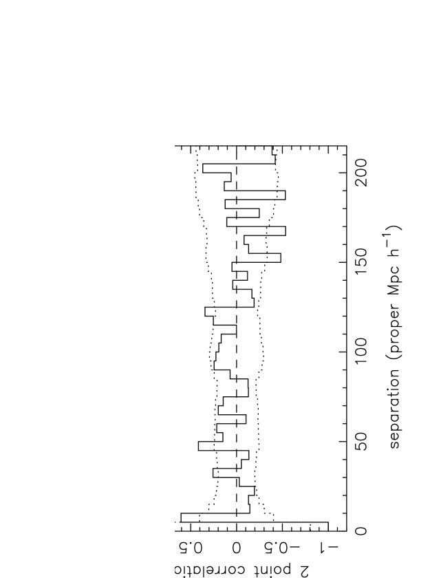
Figure 6:

Figure 7:

Figure 8: