The Average Mass and Light Profiles of Galaxy Clusters

Abstract

The systematic errors in the virial mass-to-light ratio, $M_{v}/L$, of galaxy clusters as an estimator of the field $M/L$ value are assessed. We overlay 14 clusters in redshift space to create an ensemble cluster which averages over substructure and asymmetries. The combined sample, including background, contains about 1150 galaxies, extending to a projected radius of about twice $r_{200}$. The radius $r_{200}$, defined as where the mean interior density is 200 times the critical density, is expected to contain the bulk of the virialized cluster mass. The dynamically derived $M({r_{200}})/L({r_{200}})$ of the ensemble is $(0.82\pm 0.14)\langle M_{v}/L\rangle$. The $M_{v}/L$ overestimate is attributed to not taking into account the surface pressure term in the virial equation. Under the assumption that the velocity anisotropy parameter is in the range $0\leq\beta\leq\text@frac{2}{3}$, the galaxy distribution accurately traces the mass profile beyond about the central $0.3{r_{200}}$. There are no color or luminosity gradients in the galaxy population beyond $2{r_{200}}$, but there is $0.11\pm 0.05$ mag fading in the $r$ band luminosities between the field and cluster galaxies. We correct the cluster virial mass-to-light ratio, $M_{v}/L=289\pm 50h{\rm\,M_{\odot}}/{\rm\,L_{\odot}}$ (calculated assuming $q_{0}=0.1$), for the biases in $M_{v}$ and mean luminosity to estimate the field $M/L=213\pm 59h{\rm\,M_{\odot}}/{\rm\,L_{\odot}}$. With our self-consistently derived field luminosity density, $j/\rho_{c}=1136\pm 138h{\rm\,M_{\odot}}/{\rm\,L_{\odot}}$ (at $z\simeq\text@frac{1}{3}$), the corrected $M/L$ indicates $\Omega_{0}=0.19\pm 0.06\pm 0.04$ (formal $1\sigma$ random error and estimated potential systematic errors) for those components of the mass field in rich clusters.

1 Introduction

The existence of dark matter was discovered in galaxy clusters where the velocity dispersions are nearly an order of magnitude higher than expected from the gravitational binding provided by the stellar masses of their visible galaxies (Zwicky (1933); Smith (1936); Zwicky (1937); Schwarzschild (1954)). Clusters are gravitationally bound, quasi-equilibrium systems assembled over a Hubble time via the infall of the mass in the surrounding field (van Albada (1960); Abell (1965); Peebles (1970); Gott & Gunn (1972); White (1976); Fillmore & Goldreich (1984); Bertschinger (1985)), which implies that both the dark matter and the galaxies within clusters have their origins in the field. Because clusters are large systems that draw their mass and galaxy content from regions 20$h^{-1}$ Mpc across, measurements of cluster $M/L$ values should be representative of the field value, although not necessarily identical to it because of differential galaxy evolution. The product of the field $M/L$ with the field luminosity density, $j$, is equal to the mean mass density of the universe, $\rho_{0}$ (Oort (1958)). The cosmological density parameter, $\Omega_{0}\equiv\rho_{0}/\rho_{c}$, is therefore estimated as the ratio of the cluster $M/L$ (corrected to the field) to the $(M/L)_{c}\equiv\rho_{c}/j$ for closure (e.g.  Gunn (1978)). The resulting $\Omega$ estimate has no dependence on $H_{0}$ for dynamically measured cluster masses (Gott & Turner (1976)). The purpose of this paper is mainly to correct our cluster virial mass-to-light ratio, $M_{v}/L$, (Carlberg, et al.  1996, hereafter C (96)) to the field $M/L$.

Cluster dynamical masses are usually calculated from the virial mass estimator, $M_{v}$, which has the drawback that it makes explicit assumptions about the dynamical state of the clusters. Its reliability is critically dependent on the galaxy population being in dynamical equilibrium with the cluster potential and the galaxy distribution having the same spatial distribution as the total mass distribution of the cluster. Measured virial mass-to-light ratios of clusters, $M_{v}/L$, are generally in the range $200-600h{\rm\,M_{\odot}}/{\rm\,L_{\odot}}$ (e.g.  Gunn (1978); Ramella, Geller & Huchra (1989)) which, in ratio to $(M/L)_{c}\simeq 1500h$ (Efstathiou, Ellis & Peterson (1988); Loveday et al. (1993)) indicates $\Omega\simeq 0.1-0.4$. Cluster $\Omega_{0}$ values have not generally been accepted as conclusive because there are a number of uncontrolled sources of possible systematic error. For instance, cluster galaxies with blue colors are known to have a higher velocity dispersion and are more extended than the red galaxies (Rood et al. (1972); Kent & Gunn (1982)) leading to virial mass estimates that are about a factor of four different for our dataset. The substantial color difference between cluster and field galaxies opens up the possibility that their luminosities per unit mass are quite different. The assumptions which go into the cluster $\Omega$ calculation need to be tested for their validity for a specific sample.

The possibility that the mass distributions of galaxy clusters are more extended than their constituent galaxy populations has been recognized for many years (Limber (1959)). The detection problem is that dynamical mass estimators do not have any useful sensitivity to cluster mass outside the orbits of the galaxies. A specific situation which leads to this bias is found in N-body simulations of cluster buildup in an $\Omega=1$ cosmology with a realistic amount of substructure (West & Richstone (1988); Carlberg & Dubinski (1991); Carlberg (1994); Katz & White (1993); van Kampen (1995)). In this case the simulated “galaxies” become more concentrated within the cluster than its mass. That is, the virial mass calculated from the “galaxies” systematically underestimates the total mass of the cluster in these simulations by as much as order of magnitude.

There are some observational indications of the possibility of a higher $\Omega$ than that calculated from virial masses. Detailed mass modeling for the Coma cluster gives a projected mass of $5.8\times 10^{15}h^{-1}{\rm\,M_{\odot}}$ within $3^{\circ}$ of the center (with a normal mass-to-light ratio, Kent & Gunn (1982)), whereas the virial mass is generally taken to be $2.1\times 10^{15}h^{-1}{\rm\,M_{\odot}}$ for the same region. However, this can also be ascribed to the substantial cluster to cluster variations in the shape of the velocity dispersion profile (den Hartog (1995)) due to the asphericity and substructure within individual clusters. Another indication comes from substructure, which is a complication in the analysis of clusters as individuals, but can be turned to advantage as an indirect, model dependent, $\Omega$ estimator. The results of substructure analysis remain controversial: some workers favor $\Omega\simeq 1$ (Richstone, Loeb & Turner (1992); Mohr et al. (1995)), while others suggest much smaller $\Omega$ values (Tsai & Buote (1995)).

The CNOC (Canadian Network for Observational Cosmology) cluster redshift survey is designed to derive a cluster $\Omega_{0}$ within a homogenous, self-contained, sample where we can explicitly test for systematic errors. The catalogues contain $\sim$2600 redshifts in the fields of 16 clusters (Yee, Ellingson & Carlberg (1996)) from which C (96)) derived an average $\langle{M_{v}/L}\rangle=289\pm 50h{\rm\,M_{\odot}}/{\rm\,L_{\odot}}$ (calculated with $q_{0}=0.1$). The clusters are consistent with having a universal $M_{v}/L$ value (within the errors of about 25%) independent of their velocity dispersion, mean color of their galaxies, blue galaxy content, or mean interior density. The field galaxies in the dataset, with the same corrections, over the same redshift range, yield the closure mass-to-light ratio, $\rho_{c}/j$, to be $1136\pm 138h{\rm\,M_{\odot}}/{\rm\,L_{\odot}}$. Consequently the virial mass-to-light ratio implies $\Omega_{0}=0.25\pm 0.05$ at a mean redshift of 0.32, where the error is the formal $1\sigma$ random error. In C (96) the derived $\Omega$ was erroneously corrected to a redshift zero $\Omega_{0}$. The calculation uses a co-moving volume element ($q_{0}$ dependent) and Hubble constant which are both redshift zero values which do not need further corrections.

Testing the accuracy of the virial mass was a primary consideration in the design of the CNOC observations. The data allow us to derive a radially resolved projected number density profile, $\Sigma_{N}(R)$, and a projected velocity dispersion, $\sigma_{p}(R)$ (in the following, $R$ is used for projected radius; whereas $r$ denotes the spherical co-ordinate). The sample meets the two main requirements for deriving a radially resolved mass profile which are, first, accurate control of the background, and second, enough clusters to average over the aspherical complications of individual clusters. In Section 2 we review the properties of our sample. We define scaling velocities and radii which we use in Section 3 to combine all but two “binary” clusters to create an “ensemble cluster”. This averaging increases the signal-to-noise ratio of our measurements, and is sufficient to justify the assumption of an equilibrium, spherical, cluster in the analysis. The clusters are sampled to densities in redshift space that are comparable to the field density, requiring a background subtraction which is discussed in Section 4. The mean surface density profile of galaxies within the cluster is derived in Section 5, and fitted with a spatial density profile. The projected velocity dispersion profile is derived in Section 6, and fitted to a radial velocity dispersion function for a variety of orbital shape assumptions. Using these results the mass-to-light profile is derived from Jeans equation in Section 7. In Section 8 we examine the relative colors and luminosities of field and cluster galaxies as a measurement of the differential evolution of the two populations. The corrections and error budget are presented in Section 9, followed by our conclusions and discussion in Section 10.

2 Sample and Observations

The CNOC sample is designed to create a dataset that allows as complete internal control of all aspects of the cluster $\Omega$ estimate as possible. It is essential that the sample be useful for a test of the equilibrium hypothesis and whether the virial mass is biased in some way. Furthermore the sample is used to measure differential luminosity evolution between cluster and field galaxies. On the basis of some n-body simulation data (Carlberg et al. (1994)) it was argued that these could be best met within the constraints of available observational resources with a set of a dozen or so clusters at $z\simeq 1/3$ with a total of 3000 or so accurate redshifts.

The cluster sample was chosen from the Einstein Medium Sensitivity Survey Catalogue of X-ray clusters (Gioia et al. (1990); Henry et al. (1992); Gioia & Luppino (1994)) to have a high X-ray luminosity, $L_{x}>4\times 10^{44}$ erg s^-1, which helps guarantee that the clusters are reasonably virialized and have relatively high masses, making them easier to study. The clusters chosen, Table 1, are at moderate redshifts, $0.17<z<0.55$, which has a number of advantages for mass estimation. They are sufficiently distant that they have a significant redshift interval over which the density of foreground and background galaxies are nearly uniformly sampled in redshift. At $z\simeq\text@frac{1}{3}$, a typical cluster diameter of $3$$h^{-1}$ Mpc (comoving) spans an angle of about 12′, which is sufficiently small that uniformity of photometry and sample selection is relatively easily assured. This angle is also comparable to the field size of the Canada-France-Hawaii Telescope (CFHT) Multiple-Object-Spectrograph (LeFèvre et al. (1994)), approximately 10′ square.

Observations were made at CFHT in 24 assigned nights in 1993 and 1994, of which 22 were usefully clear. The sample and observational techniques are described in detail elsewhere (Yee, Ellingson & Carlberg (1996)). The primary catalogues contain Gunn $r$ magnitudes and $g-r$ colors for 25,000 objects, of which about 2600 have velocities, on the average accurate to about 100  km s^-1. About one-third of the sample is cluster galaxies. The other two-thirds are field galaxies, although less than half of them are within the fair sample region defined by the band-limiting filter’s passband and a $\Delta z=0.01$ buffer zone added to the upper and lower cluster redshift range. For reasons of observational efficiency, the survey is not “complete” in the usual sense. Hence, each object with a redshift has calculated weights which are the inverse of the magnitude selection function and the magnitude-dependent geometric selection function (Yee, Ellingson & Carlberg (1996)). There are small changes in the cluster dynamical parameters of Table 1 from those in the global analysis (C (96)). The values here are derived using the final survey catalogues which accounts for the small changes from those given in earlier papers. All calculations in this paper assume $H_{0}=100{\rm\,km\,s^{-1}\,Mpc^{-1}}$, $\Omega_{0}=0.2$ and $\Lambda=0$, although these choices do not affect our main conclusions in any significant way.

3 Dynamical Parameters of the Clusters

The primary goal of this paper is to measure any systematic biases in $M_{v}/L$ as an estimator of the field value. This is done by independently measuring the mass and constraining differential luminosity evolution of cluster and field galaxies. We adopt the virial mass,

$$M_{v}={3\over G}\sigma_{1}^{2}r_{v},$$ (1)

as the standard estimator, where $\sigma_{1}$ and $r_{v}$ are defined below in Equations 2 and 3. The drawback of the virial mass is that it is a statistically “inefficient” estimator (Bahcall & Tremaine (1981); Beers, Flynn & Gebhardt (1990)). Its positive features are that it is completely independent of the distribution of orbital shapes and it is not unduly sensitive to background contamination. An alternate estimator is the projected mass (Bahcall & Tremaine (1981)), which we calculated but do not report. Its main drawback is that it is quite sensitive to background contamination of the data at large radii. For the standard velocity ellipsoid shape the projected mass is always larger than the virial mass, which we find below already overestimates the cluster mass. Hence, we adopted the virial mass as our standard estimator.

The first step in testing the accuracy of $M_{v}$ is to construct a low-noise, effectively spherical, “ensemble” cluster, which averages over internal substructure and the variation of projected quantities with viewing angle. Our clusters span about a factor of two in velocity dispersion and hence are not a uniform set of physically identical objects. Simply overlaying all the clusters onto a common center of mass in physical velocity and position units has some significant advantages (an approach that will be pursued in another paper), but has the disadvantage that any gradients of density or velocity dispersion tend to be blurred out. The natural scaling parameters are each cluster’s RMS velocity dispersion and the characteristic radius at which the cluster is expected to be in an effective equilibrium, which turns out to be a function of the RMS velocity dispersion, alone, within our approximation.

Deciding which galaxies in redshift space are cluster members is fundamentally ambiguous. That is, a cluster galaxy with a completely reasonable line-of-sight velocity of $1000~{}{\rm\,km\,s^{-1}}$ appears in redshift space at 10$h^{-1}$ Mpc from the cluster’s center of mass, far outside the virialized cluster and overlaying field galaxies. This complication increases in severity at large distances from the cluster center, which our sample is specifically designed to probe. One straightforward solution to this problem, which we adopt, is to explicitly subtract the mean density of field galaxies in redshift space from the cluster distribution.

The internal kinetic energy of the cluster is calculated from the characteristic velocity dispersion, $\sigma_{1}$. We iterate the classical estimator

$$\sigma_{1}^{2}=\left({\sum_{i}w_{i}}\right)^{-1}\sum_{i}w_{i}(\Delta v_{i})^{2},\qquad$$ (2)

where the $\Delta v_{i}=c(z_{i}-\overline{z})/(1+\overline{z})$ are the peculiar velocities in the frame of the cluster and $\overline{z}$ is the weighted mean redshift of the cluster. The weights are calculated from the redshift and photometric catalogues to allow for statistical incompleteness of sampling (Yee, Ellingson & Carlberg (1996)). The key to the use of this estimator is to have an objective choice of the galaxies that are likely to be cluster members. The adopted method (C (96)) is as follows. First a choice of the cluster redshift range is made from which a trial $\sigma_{1}$ is calculated. Then all galaxies between 5 and 15 $\sigma_{1}$ are used to make a background estimate, which is subtracted from the weights of the galaxies selected to be in the cluster. If the $\sigma_{1}$ calculated from the background subtracted weights is within the 68% bootstrap confidence range of the trial $\sigma_{1}$ (Efron & Tibshirani (1986)), then the procedure is stopped; otherwise, the redshift limits are increased or decreased to find a convergence.

Precisely the same galaxies as determined to be “in the cluster” from our $\sigma_{1}$ calculation are given to the iterated bi-weight estimator (Beers, Flynn & Gebhardt (1990)). The resulting estimates of the velocity dispersion are, on the average, $1.073\pm 0.019$ times larger than from our method. We find below that the global mean velocity dispersion of the combined dataset, normalized with our $\sigma_{1}$ values, is $1.05\pm 0.04$, whereas it should be unity, which is consistent with either scheme for calculating the velocity dispersions. Since the outcome of this investigation is that $M_{v}$ is biased upwards, the bi-weight calculation would lead to a further increase in the bias.

For each cluster a “ringwise” estimate of the virial radius of the observed distribution is calculated (see C (96) for details):

$${1\over r_{v}}={2\over\pi}\left(\sum_{i}w_{i}\right)^{-2}\sum_{i<j}{w_{i}w_{j}{2\over{\pi(r_{i}+r_{j})}}K(k_{ij})},$$ (3)

where $k_{ij}^{2}=4R_{i}R_{j}/(R_{i}+R_{j})^{2}$ and $K(k)$ is the complete elliptic integral of the first kind in Legendre’s notation (Press et al. (1992)). The angular extent of the sample is set by the observed field size. The redshift range is as found in the velocity dispersion calculation.

The goal is that our data will include the entire virialized mass of the cluster. Analytic models (Gott & Gunn (1972)) and simulation data (Cole & Lacey (1996); Zembrowski & Carlberg (1996)) find that the virialized mass is generally contained inside the surface where the mean interior density is $200\rho_{c}$ at the redshift of the cluster. The mean interior density within our measured $r_{v}$ is

$${\overline{\rho}(r_{v})\over{\rho_{c}(z)}}={1\over{\rho_{c}(z)}}{{3M_{v}}\over{4\pi r_{v}^{3}}}.$$ (4)

In terms of the measured dynamical parameters this is

$${\overline{\rho}(r_{v})\over{\rho_{c}(z)}}={{6\sigma_{1}^{2}}\over{H^{2}(z)r_{v}^{2}}},$$ (5)

where the Hubble constant at $z$ is $H^{2}(z)=H_{0}^{2}[\Omega_{0}(1+z)^{3}+\Omega_{R}(1+z)^{2}+\Omega_{\Lambda}]$ (Peebles (1993)). Normally we take $\Omega_{0}=0.2$, $\Omega_{\Lambda}=0$ and $\Omega_{R}=1-\Omega_{0}$ for an open FRW model. The mean density inside $r_{v}$ serves as a check as to whether the radial extent of the cluster is sufficiently sampled to determine a virial radius that includes most of the virialized mass. Table 1 gives the values for $r_{v}$, $\sigma_{1}$, and $\overline{\rho}(r_{v})/\rho_{c}(z)$, in columns 3, 4 and 5, respectively. The sampling over-density $\overline{\rho}(r_{v})/\rho_{c}(z)$ varies substantially from cluster to cluster, which mainly indicates the radial extent of our coverage of a given cluster. The observations used here extend beyond $r_{200}$ for most clusters. The exceptions are MS1006$+$12, MS1008$-$12, and MS1455$+$22 where the data extend to about 2/3 to 3/4 of $r_{200}$.

The cluster’s virial mass to k-corrected Gunn $r$ luminosity, $M_{v}/L$, and its errors are given in columns 6 and 7 of Table 1. The numbers are slightly different than those found in C (96) because these results are based on the finalized catalogues.

To calculate $r_{200}$, the radius where the mean interior density is $200\rho_{c}(z)$, requires an assumption as to how the mass is distributed. One possibility is that the mass is strongly concentrated to the center of the cluster such that all the mass measured by $M_{v}$ is inside the measured $r_{v}$, in which case,

$${r^{\prime}_{200}}=r_{v}\left[{{\overline{\rho}(r_{v})}\over{200\rho_{c}(z)}}\right]^{1/3}.$$ (6)

This definition of $r_{200}$ is not particularly appropriate when $\overline{\rho}/\rho_{c}(z)<200$, as it is for our best sampled clusters, because the cluster galaxies, and presumably the mass as well, extend beyond $r_{200}$. A superior $r_{200}$ is calculated assuming a density-radius model which is extrapolated to the desired overdensity. Simplicity, and a great deal of work on clusters of galaxies and the properties of dark halos in general, suggests that the first approximation for the density-radius relation is the singular isothermal sphere, $\rho\propto r^{-2}$, in which case we define,

$${r_{200}}=r_{v}\left[{{\overline{\rho}(r_{v})}\over{200\rho_{c}(z)}}\right]^{1/2},$$ (7)

or equivalently,

$${r_{200}}={\sqrt{3}\sigma_{1}\over{10H(z)}}.$$ (8)

Note that ${r^{\prime}_{200}}\propto\sigma_{1}^{2/3}r_{v}^{1/3}$ and ${r_{200}}\propto\sigma_{1}$. That is, $r_{200}$ is independent of the angular extent of the sampling, in so far as the cluster’s $\sigma_{1}$ value has no radial dependence, which for the shallow gradients of the velocity dispersion profile found below is effectively true. At $z=\text@frac{1}{3}$ a low density, flat universe gives a value of $r_{200}$ about 13% larger than in a open universe.

Values of ${r^{\prime}_{200}}$ and $r_{200}$ are given in columns 8 and 10 of Table 1 in units of physical $h^{-1}$ Mpc for our cluster sample. For our sample these two $r_{200}$ estimates have very similar values, so the results are not sensitive to the mass model. The jacknife error estimates for ${r^{\prime}_{200}}$ and $r_{200}$ in $h^{-1}$ Mpc are given in columns 9 and 11, respectively. All of the following analysis will use $r_{200}$ as the scaling radius.

Two of the clusters, MS0906+11 and MS1358+62, are strong binaries, the first having an ill determined velocity dispersion and the second having a massive substructure on one side moving at 1000  km s^-1 relative to the cluster center. These are dropped from all further use in this paper. The scaled velocity-radius data for the remaining clusters are displayed in Figure The Average Mass and Light Profiles of Galaxy Clusters plotted using the brightest cluster galaxies (BCGs) as the projected center and the weighted average redshift as the velocity center.

4 Background Subtraction

All of the cluster properties presented in this paper are measured using galaxies with redshifts. The clusters typically extend over a velocity range of $5000{\rm\,km\,s^{-1}}$, which in redshift space causes orbitting cluster galaxies to be intermingled with field galaxies within a 50$h^{-1}$ Mpc distance interval around the cluster. Background and foreground galaxies that are projected into the redshift space of the cluster must be statistically removed. This survey was deliberately placed at moderate redshift to give a field sample over a considerable redshift column from which the background density can be accurately measured. The background density is measured in the normalized velocity-radius space of Figure The Average Mass and Light Profiles of Galaxy Clusters. It should be noted that the sampling in Figure The Average Mass and Light Profiles of Galaxy Clusters varies substantially with both velocity and radius which is addressed with redshift cutoffs and magnitude and position dependent weights (Yee, Ellingson & Carlberg (1996)). The background and foreground are folded on top of one another within the unbiased redshift sample range of the band limiting filters which removes any linear gradients present in the redshift distribution.

There are two approaches to background subtraction used in the following calculations. For the surface density calculation we use the straightforward average over the sky area observed. The velocity dispersion calculation takes a more cautious approach to background subtraction. A resolved background is derived in precisely the same range of projected radii for which ${\sigma_{p}}(R)$ is calculated. The advantage of this approach is that the contamination of the cluster velocity profile with various nearby groups of galaxies is subtracted in the range of projected radii where they contribute to the background. Furthermore, the ${\sigma_{p}}(R)$ calculated from non-overlapping radial ranges are completely independent of each other.

5 The Average Density Profile

The surface number density profile of the average cluster, $\Sigma_{N}(R)$, is the projection over velocity onto the radius axis, $R$, of the data of Figure The Average Mass and Light Profiles of Galaxy Clusters. To find $\Sigma_{N}(R)$, we sum the statistical weights (which correct for nonuniform sampling, Yee, Ellingson & Carlberg (1996)) for objects within 3$\sigma_{1}$ of zero velocity, divide by the bin area, and subtract the mean background. We prefer the BCGs as the projected centers (Bird (1994)), but repeat most of the analysis using the peak of the smoothed density profile as the centers, which gives a useful view of systematic effects in the analysis.

The mean background volume density in velocity space, $\overline{\rho}_{b}^{\dagger}$, is calculated by summing over the entire range of $R/{r_{200}}$ using the background in the velocity range of 5 to 25 $\sigma_{1}$. We find that $\overline{\rho}_{b}^{\dagger}=0.0065\pm 0.0008$, in units of the normalized total numbers per $\sigma_{1}$ per ${r_{200}}^{2}$. Figure The Average Mass and Light Profiles of Galaxy Clusters shows the variation of the average background density with velocity separation (in normalized units) from the cluster. Between 3 and 6$\sigma_{1}$, the background calculated from the full sample (left panel) is higher than expected for a high velocity tail like a Gaussian. This excess is statistically significant at about the 3 standard deviation level, and results from various small groups that happen to be behind the low redshift clusters. The right panel of Figure The Average Mass and Light Profiles of Galaxy Clusters shows the background calculated after the 7 clusters with $z\leq 0.27$ are dropped. The rapid decline of clustering with redshift leads to a smoother distribution in redshift in the right panel. The mean background is calculated over the entire 5 to 25$\sigma_{1}$ interval for the full sample, so a local excess makes little difference. As a sidelight we note that near the cluster center, 1-3$\sigma_{1}$, the velocity distribution is possibly somewhat “squarer” than a Gaussian distribution. That is, for a Gaussian the ratio of the numbers between 1 and 2$\sigma_{1}$ and 0 to 1$\sigma_{1}$ is about 1/3, whereas we have more than 1/2. This is likely an indicator that the cluster velocity ellipsoids are somewhat radially anisotropic (Dubinski (1993); Crone, Evrard & Richstone (1994)).

To check the sensitivity of the derived $\Sigma_{N}(R)$ to the assumed background level we repeat the calculation using values for $\overline{\rho}_{b}^{\dagger}$ of 0.0048 and 0.0082, which are 2 standard deviations from the mean value. The only part of the profile substantially affected is beyond $r_{200}$, with alternate values being just within the 1 standard deviation range of the estimated density at that point. That is, for our adopted bin widths the statistical error due to sample size generally exceeds the uncertainty in the background subtraction. The fitted profiles described below have scale radii altered by 1.5% for a 26% variation of the background. We conclude that the background subtraction is not a dominant source of error for $\Sigma_{N}(R)$.

The background subtracted $\Sigma_{N}(R)$ are displayed in Figure The Average Mass and Light Profiles of Galaxy Clusters and tabulated in Table 2. The vertical normalization of $\Sigma_{N}(R)$ is a fixed, but arbitrary, value. In Table 2 the number density $\Sigma_{0}$ (column 2) is measured about the BCG, and $\Sigma_{p}$ (column 4) is measured about the peak of the 45″ Gaussian smoothed density map. Within $0.1{r_{200}}$ of the center the density profile is strongly dependent on the choice of center. Because there is usually no galaxy at the point of peak density, there is a slight dip in the central surface density when measured about the peak of the smoothed density distribution. The choice of center makes little difference to the measured $\Sigma_{N}(R)$ at radii beyond $0.1{r_{200}}$, approximately 100$h^{-1}$ kpc, but it does affect fits to a specific model. The point of peak density generally has sufficiently large errors that it could be consistent with being at the BCG, hence we always prefer the BCG center for physical reasons (Bird (1994)). Outside of $2{r_{200}}$ the surface density is comparable to the background but the data are very sparse, which together cause the surface density at large radius to be quite uncertain. No data beyond $2{r_{200}}$ are used in the velocity dispersion analysis. The surface luminosity density profile was also derived; but, being weighted to the brightest galaxies, it is a noisier quantity than the number density. We find that the luminosity density profile shape is essentially the same as the density distribution.

The spatial galaxy number density as a function of radius, $\nu(r)$, is needed to compare the galaxy number profile with the cluster mass profile. The relation between the volume density and the surface density is,

$$\Sigma_{N}(R)=2\int_{R}^{\infty}\nu(r){r\over\sqrt{r^{2}-R^{2}}}\,dr.$$ (9)

A statistically adequate, analytically convenient, model that describes these data is the Hernquist (alternatively designated as an $\eta=2$) model (Hernquist (1990); Tremaine et al. (1994)). We fit the data centered on the BCG of Figure The Average Mass and Light Profiles of Galaxy Clusters to the projection of the volume density model,

$$\nu(r)={A\over{r(r+a)^{3}}}.$$ (10)

This procedure for finding a $\nu(r)$ consistent with the $\Sigma_{N}(R)$ data is not unique, there being both the minor variation of using one of several other entirely reasonable fitting functions, or, adopting a completely different approach such as the non-parametric, maximum likelihood method (Merritt & Tremblay (1994)) modified to allow for background subtraction. The function $\nu(r)=Ar^{-1}(r+a)^{-2}$ (Navarro, Frenk & White (1995)) is also a statistically acceptable fit with a slightly increased $\chi^{2}$. Our measured $\Sigma_{N}(R)$ falls faster than this function predicts at large $R$, but at these radii our measurement is relatively uncertain.

Fitting the surface density data with Equation 10 finds that $a=(0.66\pm 0.09){r_{200}}$ for the clusters centered on their BCGs. The reduced chi-squared statistic, $\chi^{2}/n_{f}$, is 0.74 for $n_{f}=17$ degrees of freedom, which is an acceptable fit. Using the $\Sigma_{N}(R)$ measured about the peak light gives a considerably larger scale radius, $a=(0.97\pm 0.10){r_{200}}$, with $\chi^{2}/n_{f}=1.01$. This larger value of $a$ is at least in part due to a blurring of the density profile by statistical errors in measuring the position of peak number density. Although we believe it is a less appropriate choice for the cluster centers for these data, we carry it along in the analysis as an indicator of systematic errors.

6 The Velocity Dispersion Profile

The measurement of ${\sigma_{p}}(R)$ is a second moment of the velocity distribution about the local mean velocity at projected radius $R$, although the choice of central moment makes essentially no difference to the result. The projected velocity dispersion at $R$, ${\sigma_{p}}(R)$, is calculated using an iterative clipping of the high velocity dispersion tails with a technique similar to that used for the RMS velocity dispersion in C (96), where $\sigma_{1}$ is calculated from the background subtracted data within $n_{c}\sigma$ of zero velocity, where $n_{c}=3$. The iteration begins with ${\sigma_{p}}(R)=1$ in the $\sigma_{1}$ normalized velocities. For the next four iterations the ${\sigma_{p}}(R)$ from the previous iteration is used for clipping. For a 10% change in the clipping level, $n_{c}$, the resulting velocity dispersion changes about 1% at large radii. The error flags are calculated from a full bootstrap resampling of both the cluster and field data.

Rather than radially binning the data, we use a moving average, which includes all galaxies, both cluster and field. Table 3 gives the results with a 51 point moving average which are plotted in Figure The Average Mass and Light Profiles of Galaxy Clusters at intervals of 0.1 in $r_{200}$. These points are always independent for 51 point averaging. Averages using 31 to 201 points give consistent results, the 31 point result being quite noisy, and the 201 point beginning to smooth the velocity dispersion gradient. The results of a 101 point moving average are shown in Figure The Average Mass and Light Profiles of Galaxy Clusters. For 101 point averaging the error flags are not independent outside of $0.4{r_{200}}$.

The random errors of the derived ${\sigma_{p}}(R)$ of the ensemble are dominated by cluster to cluster fluctuations. Within an individual cluster (for instance A2390) the random errors are substantially smaller, but there are large differences in velocity dispersion profiles from cluster to cluster (den Hartog (1995)) which we attribute to projection effects and substructure. At large radii, dynamical measurements from a single cluster likely do not give reliable enclosed masses because of the complications of infall, triaxiality and substructure. The idea of creating the ensemble cluster is of course to diminish these systematic variations to the level where an effectively spherically symmetric average profile emerges.

To derive a $\sigma_{r}(r)$ which is consistent with the observed ${\sigma_{p}}(R)$ we use the same approach as we used for the density profile. That is, we choose a reasonable functional form, then adjust 2 parameters, a scale length and a normalization, until its calculated projection,

$${\sigma_{p}}^{2}(R)\Sigma_{N}(R)=\int_{R}^{\infty}\nu(r)\sigma_{r}^{2}(1-\beta{R^{2}\over r^{2}}){r\over\sqrt{r^{2}-R^{2}}}\,dr.$$ (11)

minimizes the $\chi^{2}$. In this equation $\beta=1-\sigma_{\theta}^{2}/\sigma_{r}^{2}$ is the velocity anisotropy parameter. For the purposes of this paper $\beta$ will be taken to be a constant, although we do use a range of values.

The adopted $\sigma_{r}(r)$ function should be finite at the origin, at large $r$ it should tend to a Keplerian $r^{-1/2}$ for a convergent mass distribution, and it should be a simple smooth function in between. It is important that this function not assume that the galaxy populations are self-consistent with the mass density of the potential. We adopt the simple form,

$$\sigma_{r}^{2}(r)={B\over{b+r}},$$ (12)

for the radial velocity dispersion. This function, with B=$\text@frac{1}{4}$ and assuming $b=a$, is the solution of the Jeans Equation (Equation 13 below) for $\beta=\text@frac{1}{2}$ and $A=1/(2\pi)$ in our assumed $\nu(r)$. The scale lengths $b$ and $a$ are fitted separately, usually finding that $b$ is larger than $a$.

The nonlinear fitting procedure requires that the errors be symmetric about the observed value, so we take the larger of the upper and lower error range at each point. The fit is done assuming $\beta=0,0.25,0.5$ and $0.75$. The projected fit and the 51 point data are shown in Figure The Average Mass and Light Profiles of Galaxy Clusters. The $\chi^{2}/n_{f}$ of the two parameter fit, an amplitude and length scale, is $0.48$ for all $\beta$ values.

7 Mass-to-Light Profiles

To compare the relative distribution of mass and light we integrate our fitted $\nu(r)$ to give $L(r)$, the “light profile” (actually a number density profile), which is converted to a mass profile using a normalized global $M_{v}/L$, calculated in the same manner as for the individual clusters. Then we compare the mass predicted by the light-traces-mass assumption to the $M(r)$ derived from the fitted $\sigma_{r}(r)$ and $\nu(r)$ using Jeans Equation,

$$M(r)=-{\sigma_{r}^{2}r\over G}\left[{{d\ln{\sigma_{r}^{2}}}\over{d\ln{r}}}+{{d\ln{\nu}}\over{{d\ln{r}}}}+2\beta\right].$$ (13)

We will usually refer to the mass derived from this equation as $M_{SHD}(r)$, the stellar hydrodynamical mass.

It must be borne in mind that Equation 13 is a moment of the Collisionless Boltzmann Equation, and will not necessarily give a physical result for all $\beta$, being particularly susceptible to failure for very radial orbits (Binney & Tremaine (1987); Hernquist (1990)). In addition, radial models are usually dynamically unstable to the radial orbit instability (Barnes, Goodman & Hut (1986); Palmer & Papaloizou (1987)). However, the galaxies are only tracers, so in principle they could be on much more radial orbits than the underlying dark matter. On the other hand, it seems likely that galaxies orbiting past the center may be tidally destroyed or simply well mixed so that the galaxy velocity ellipsoid near the center may become less radial than the dark matter.

7.1 Dynamical Modeling Details

Equation 13 is integrated with the boundary condition that $\sigma_{r}\rightarrow 0$ as $r\rightarrow\infty$. Alternative boundary conditions are that the velocity dispersion goes to zero at the turnaround radius (Gott & Gunn (1972)), or, that there is an outer region of nearly radial infall which makes a transition to virialized motion (den Hartog (1995)). N-body simulations (e.g.  Crone, Evrard & Richstone (1994); Cole & Lacey (1996); Zembrowski & Carlberg (1996)) show that on the average, the approximation that the virialized motion continues to $r_{200}$ is a good one. For constant $\beta$ Equation 13 has a formal solution,

$$\sigma_{r}^{2}(r)={{\int_{r}^{\infty}GM(x)\nu(x)x^{(2\beta-2)}\,dx}\over{\nu(r)r^{2\beta}}}.$$ (14)

Satisfying the Jeans equation is a necessary condition for an equilibrium to exist, but it is not sufficient and is certainly not a guarantee that a spherical distribution is dynamically stable. Models with a constant $\beta\gtrsim\text@frac{2}{3}$ are unphysical, because the implied mass is negative in the inner regions (very radial orbits lead to $\nu(r)\propto r^{-2}$, not the $r^{-1}$ here). This, along with the results of numerical simulations, leads to our preference for $0\leq\beta\leq\text@frac{1}{2}$. The model lines plotted on Figure The Average Mass and Light Profiles of Galaxy Clusters are for $\beta=0,\text@frac{1}{2}$ and 1, assuming $M(r)\propto L(r)$ in Eq. 14, using the fitted $\nu(r)$ from Eq. 10, and normalizing the projected RMS velocity dispersion over the observed radial range to the observed value.

The numerical complication in deriving $M(r)$ from Equation 13 is that the logarithmic gradients $d\ln{\sigma_{r}^{2}}/d\ln{r}$ and $d\ln{\nu}/d\ln{r}$ must be calculated. Numerically evaluating these gradients from the data requires some form of smoothing to be stable, which our fits to smooth functions effectively accomplish. We will carry the errors of the projected $\sigma_{p}$ data through the analysis to help give an assessment of the result.

7.2 Velocity Ellipsoid Anisotropy

The radial dependence of the shape of the velocity ellipsoid, as defined by the value of $\beta$, is not empirically known for this sample, although this does not introduce the same uncertainty as it does for finding central dark masses. As the velocity ellipsoid becomes more and more radial at large radii, the mass implied for a measured $\sigma_{p}$ increases. The inferred mass has nearly a full order of magnitude uncertainty when a velocity dispersion is available at only a single point with no knowledge of the shape of the velocity ellipsoid (Merritt (1984); Richstone & Tremaine (1984); The & White (1986)). Because we have measured the velocity dispersion over a wide radial range the uncertainty due to velocity dispersion anisotropy becomes quite small, as shown below.

N-body simulations of objects that form via collapse find that $\beta\geq 0$ (Richstone & Tremaine (1984)), although it is clear now that “vacuum” boundary conditions give far more velocity anisotropy than is realistic in a cosmological setting (Dubinski (1993)) where substantial external torques provide angular momentum to large radius orbits. Furthermore, strongly radial models are unstable (Barnes, Goodman & Hut (1986); Palmer & Papaloizou (1987)), although galaxies, being nearly massless within a cluster, could have a different velocity ellipsoid than the dark matter. For the nearly power law hierarchical clustering that characterizes the growth of clusters in model universes one expects that the velocity ellipsoid will have only a weak radial dependence, because cluster buildup is self-similar. This is borne out in n-body simulations (Dubinski (1993); Crone, Evrard & Richstone (1994); Zembrowski & Carlberg (1996)) which find $0\leq\beta\leq 0.5$ over the radial range of interest for a wide range of $\Omega_{0}$ and clustering models. The depletion of HI in Coma spirals suggests (Pryor & Geller (1984)) that their velocity ellipsoid is not strongly radial, and is consistent with being isotropic.

7.3 The Average Mass-to-Light Ratio within $r_{200}$

A test of the accuracy of the virial mass as an estimator of the total mass virialized in the cluster is whether the product of the virial mass-to-light ratio computed from our average cluster and the integrated interior luminosity, $L(r)$, is equal to the stellar hydrodynamical mass, $M_{SHD}(r)$, derived from Eq. 13. That is, we derive the virial mass bias, $b_{Mv}(r)$, from

$$b_{Mv}(r)={{M_{SHD}(r)}\over{L(r)}}{\tilde{L}\over\tilde{M}_{v}},$$ (15)

where $L(r)$ is simply the volume integral of $\nu(r)$. The normalization of $L(r)$, $\tilde{L}$, is arbitrary since it cancels in Eq. 15. The normalizing virial mass, $\tilde{M}_{v}$, is derived for the ensemble cluster in the same way as for the individual clusters. Two aspects of $b_{Mv}(r)$ are of primary interest. First, $b_{Mv}({r_{200}})$ should be unity if the $\tilde{M}_{v}/\tilde{L}$ calculated from the average cluster is an unbiased estimator for all material inside $r_{200}$, the radius expected to contain most of the virialized mass. Second, the radial gradient of $b_{Mv}(r)$ measures to what degree light traces mass in the average cluster. The first issue is the one of most relevance for the problem of $\Omega$ estimation. It should be noted that whatever the value of $b_{Mv}(r)$ turns out to be here, it is a quantity that is meant to give the systematic error in measuring cluster mass using red selected galaxies in rich, reasonably relaxed clusters. It would be inappropriate to apply the same factor to merging clusters or a galaxy sample selected to emphasize high star formation rates, for example.

The galaxy number density profile, which we will call the light profile, is normalized to a mass using a mass-to-light ratio calculated in the same manner as done for our clusters individually. There are two complications in this calculation which need to be examined. First, the clusters are not all sampled to the same fraction of $r_{200}$. Second, both the $r_{v}$ and the total light are calculated without any allowance for background contamination. To investigate these effects we calculate $\tilde{M}_{v}/\tilde{L}$ using the mean profile, both with and without background subtraction, limiting the data at various $R_{max}/{r_{200}}$. The results are shown in Figure The Average Mass and Light Profiles of Galaxy Clusters.

Remarkably, the ratio $\tilde{M}_{v}/\tilde{L}$ is almost entirely independent of background contamination and sampling radius, once $R_{max}/{r_{200}}\gtrsim 0.5$. The lower line on the figure is made using the surface density without background subtraction, which causes $\tilde{r}_{v}$, hence $\tilde{M}_{v}$, to be overestimated, but the summed luminosity is also overestimated. The pleasing result for this sample is that the two overestimates almost exactly cancel out so that $\tilde{M}_{v}/\tilde{L}$ calculated in the usual manner has no sensitivity to background. Furthermore, $\tilde{M}_{v}/\tilde{L}$ has very little dependence on the sky coverage of the cluster, provided that the data extend beyond $0.5{r_{200}}$. Figure The Average Mass and Light Profiles of Galaxy Clusters shows that the directly calculated average $\tilde{M}_{v}/\tilde{L}$ is high in the inner regions, but then drops to a very stable value at large radius. The normalizing virial mass is $\tilde{M}_{v}=3\tilde{\sigma}_{1}^{2}\tilde{r}_{v}$, where $G=1$ and the parameters are the measured $\tilde{\sigma}_{1}$ and $\tilde{r}_{v}$ for the combined cluster data. We use the quantities for the full sample, with background subtraction, although this choice makes little difference to the results. With this normalization, $b_{Mv}({r_{200}})$ should be unity if $M_{v}$ is unbiased.

7.3.1 Virial Mass Bias

The internal $M_{v}/L$ bias, $b_{Mv}(r)$, from Eq. 15 is displayed as a function of radius in Figure The Average Mass and Light Profiles of Galaxy Clusters for $\beta=0,0.25,0.5$ and $0.75$. The bias would be unity everywhere if the product of $\tilde{M}_{v}/\tilde{L}$ and $L(r)$ was equal to the stellar hydrodynamical mass. Note that if $\beta\gtrsim 2/3$ the implied mass is negative at small radius.

The primary goal of this paper is to correct the virial mass-to-light ratio to the field $M/L$ value. The average virial mass bias for the bulk of the virialized system estimates the systematic offset in the virial mass, and is reasonably estimated as the value of $b_{Mv}$ evaluated at $r_{200}$, displayed in Figure The Average Mass and Light Profiles of Galaxy Clusters as a function of the assumed $\beta$. Because the gradient is small the exact radius used does not make a big difference. The error in $b_{Mv}({r_{200}})$ is calculated from the error in the fit to the $B$ coefficient in $\sigma_{r}(r)$, the error in the other quantities being negligible in comparison. The 3 symbols are for absolute magnitude cutoffs of $M_{r}^{k}=$-18.5, -19.0, and -19.5 mag, respectively, of the entire calculation. The points offset in $\beta$, with the dashed error flags, use the peak density as the centers and are always poorer fits, hence have larger errors. These points are included to illustrate the small systematic differences. All the results are statistically identical.

We find $M_{v}$, as normally calculated, is always an overestimate of the mass, whose value is weakly dependent on the assumed $\beta$ value. For this sample the bias is minimal (i.e.  $b_{Mv}$ closest to unity) near $\beta<\text@frac{1}{2}$ for which it is equal to $0.82\pm 0.14$. All $\beta$ give statistically consistent bias values, although there is clear trend of decreasing $b_{Mv}$ with increasing $\beta$.

7.3.2 The Mass-to-Light Ratio Gradient

The inferred radial gradients of $b_{Mv}$ for different $\beta$ are shown in Figure The Average Mass and Light Profiles of Galaxy Clusters. The gradient is calculated from the slope of the lines in Figure The Average Mass and Light Profiles of Galaxy Clusters. Only for very radial orbits, $\beta\geq\text@frac{2}{3}$, is there even a mildly significant rising mass-to-light ratio with radius, and those are the models with negative central mass. The gradients are sufficiently small that for a wide range of $\beta$ they are consistent with there being no gradient of $M/L$. In no case are the gradients sufficiently large that there is any possibility that the cluster has a dark matter halo that is significantly more extended than the visible galaxies.

7.4 A Model Calculation of the Virial Mass Bias

We have found that the virial mass, as we have calculated from the data, is about a 20% overestimate of the true mass. The origin of this factor needs to be quantitatively understood. We believe that this bias is simply the approximation that the surface pressure term in the virial equation is zero. For our fitted functional forms for the density profile and the velocity dispersion profile, (Equations 10 and 12, respectively), we can provide an estimate of the expected “truncation bias”.

Truncating a density profile of the form Eq. 10, $\rho(r)=Ma(2\pi r)^{-1}(r+a)^{-3}$, will cause the true mass contained within that radius to be overestimated, as quantified below. The potential energy scalar, $W(x)$, of the density distribution truncated at $x$ is,

$$4\pi\int_{0}^{x}\rho M(r)r\,dr={\frac{GM^{2}{x}^{3}\left(x+4a\right)}{6a\,\left(x+a\right)^{4}}},$$ (16)

Calculating the virial radius as $r_{v}=M(x)^{2}/W(x)$ we find that

$$r_{v}(x)={\frac{6\,xa}{x+4a}}.$$ (17)

The estimated virial radius is $6a$ if the distribution is sampled to infinity distribution, whereas for our combined clusters we have measured the virial radius to be $3.9a$ (using the $a$ found from the fit of the distribution with background subtraction). This is consistent, within the errors, with our truncation radius $x\simeq 4a$ and Eq. 17 for the combined sample. The clusters as individuals all have truncation radii less than or equal to this.

If the galaxy distribution follows the mass density the mass contained within $x$ is estimated from the “classical” virial theorem relating the kinetic energy, $T(x)$, $W(x)$, and the surface term, $3PV(x)$, through $2T(x)+W(x)=3PV(x)$, as $M_{v}(<x)=2G^{-1}T(x)r_{v}(x)/M(x)$. The usual assumption for dynamical systems is that $3PV(x)$ is evaluated as $x\rightarrow\infty$, where it is zero. This is not correct in detail for clusters of galaxies, where this term is a significant correction.

For the particular case of $\beta=\text@frac{1}{2}$, it was noted above that the solution of Jeans Equation is $\sigma_{r}^{2}(r)=GM/[4(a+r)]$. Hence the truncated kinetic energy, $T(x)$, is,

$$2\pi(3-2\beta)\int_{0}^{x}\rho(r)\sigma_{r}^{2}(r)r^{2}\,dr={\frac{GM{x}^{2}\left(x+3a\right)}{12a\,\left(x+a\right)^{3}}}.$$ (18)

For the case of the mass being distributed like the galaxies, the ratio of the estimated mass contained within $x$ to the true mass contained is,

$${{M_{v}(<x)}\over{M(x)}}={\frac{\left(x+3a\right)\left(x+a\right)}{x\left(x+4a\right)}}.$$ (19)

Note that this expression could also be derived from $2T+W=3PV$, as discussed in C (96). At any finite radius this estimated mass is greater than the true global value. At $x=a$, $2a$, $3a$ and $4a$ it evaluates to 8/5, 5/4, 8/7 and 35/32, respectively. That is, the mass estimated from the averaged distribution is expected to overestimate the true value by about 10 to 20%. Clusters that are not sampled to large radii will have a larger truncation bias but smaller background contamination in the projected quantities. The data in most of our clusters extend to 1 to 2 $r_{200}$, roughly consistent with the measured $b_{Mv}$.

8 The Radial Gradient of Galaxy Populations

A crucial step in the derivation of $\Omega$ from cluster $M/L$ values is to correct for any differential luminosity evolution between the cluster and field galaxies. The luminosities of galaxies per unit total mass can, in principle, either increase or decrease depending on what happens when galaxies fall into a cluster. The empirical evidence is that once galaxies have spent some time in rich, high X-ray luminosity clusters like those in our sample, star formation largely ceases. However, there are at least two routes to this end point for a gas rich disk galaxy. Galaxies entering the cluster could have their gas largely stripped away, or, a burst of star formation upon cluster entry could boost luminosity prior to depleting the gas. In either of these cases, lowering the star formation rate leads to a decrease in a galaxy’s luminosity by an amount that depends on its entire star formation history. Galaxy merging always decreases numbers, but can lead to luminosity increases if accompanied by star formation. All these possibilities are testable in one way or another, and some substantial constraints on differential evolution can be imposed using the data at hand.

It is well known that the fraction of cluster galaxies with blue colors is a strongly increasing function of redshift, the Butcher-Oemler effect (Butcher & Oemler (1984); Yee et al. (1995)). It should be noted that cluster galaxies are, on the average, never bluer than field galaxies, implying that, on the average, star formation always declines into a cluster. If the infall of field galaxies into clusters induces a temporary increase star formation and hence increases cluster galaxy luminosities relative to the field, then it should be apparent as a change in the color distribution (and the strength of the [OII] lines). This is not seen in our data (e.g.  Abraham et al. (1996)). On the basis of these considerations we expect that cluster galaxies are of intrinsically lower luminosities than the field galaxies.

Our sample of galaxies extends from the cluster center to the distant field, allowing population gradients to be examined as a function of a redshift space radial variable, $s$. A convenient definition of such a variable is based on our normalized co-ordinates, where velocity differences are scaled to $\sigma_{1}$ and projected radial co-ordinates are scaled to $r_{200}$, so that the dimensionless redshift space separation from the center is $s^{2}=R^{2}/{r_{200}}^{2}+(\Delta v)^{2}/\sigma_{1}^{2}$, where $R$ is the projected radius from the center and $\Delta v$ is the rest-frame velocity difference from the average redshift. Note that at large $s$ the galaxies come exclusively from the redshift direction. Figure The Average Mass and Light Profiles of Galaxy Clusters shows the color-radius relation of the full sample. All galaxies with k-corrected absolute $r$ magnitude, $M_{r}^{k}$, brighter than $-19$ mag are plotted. The colors are corrected to an empirically normalized redshift-independent color,

$$(g-r)_{z}=(g-r)[1.2+2.33(z-0.3)]^{-1}$$ (20)

(C (96)). We note that there is no color gradient in the field, but one appears at $s\simeq 2$, where we expect galaxies to enter the virialized region of the cluster. There is no evidence in the colors for excess star formation at the edge of the cluster; indeed, there are no cluster galaxies systematically bluer than field galaxies. Hence, the distribution of galaxy color with radius (Fig. The Average Mass and Light Profiles of Galaxy Clusters) is consistent with infalling galaxies terminating their star formation with little or no “starbursting” once they enter the cluster, as detailed analysis of the CNOC data for A2390 has demonstrated (Abraham et al. (1996)).

A sample extending to a larger projected radius is needed to directly demonstrate kinematic evidence for infall of galaxies into the clusters. However, given the gravitational mass of the cluster, the turnaround radius is straightforwardly derived (Gott & Gunn (1972); Kent & Gunn (1982)) such that field galaxies must be falling into the cluster out to the turnaround radius, approximately $4.6{r_{200}}$ for the model profile here. To a significant degree the cluster must be composed of former field galaxies. In such an infall scenario the cluster galaxies statistically share the star formation history of the field, prior to cluster entry.

The only gross difference between clusters and field is that clusters contain an unusual population of luminous central galaxies. The BCGs only make a difference at small $s$, and generally contribute well less than 10% of the light. In spite of the substantial radial color gradient of Figure The Average Mass and Light Profiles of Galaxy Clusters there is very little change in the $r$ band luminosity distribution of Figure The Average Mass and Light Profiles of Galaxy Clusters. Measurements of the surface brightness evolution of both disks and bulges arrives at the conclusion that the amount of differential evolution between the field and the cluster luminosities is relatively small (Schade et al.  1996a ; 1996b ).

There is no significant difference in the field galaxy luminosities or colors at any radius beyond $2{r_{200}}$, as shown in Figure The Average Mass and Light Profiles of Galaxy Clusters. That is, the field galaxies near the cluster appear to be indistinguishable from those far away. A generic prediction of “natural bias” models of cluster galaxy formation is that the galaxies that eventually fall into the cluster should form earlier because the overdensity of the incipient cluster speeds up the local time scale relative to the mean universe. Possibly this leads to a higher rate of conversion of gas to stars, causing cluster galaxies to be more luminous than their counterparts in the field. The color gradient appears at about $2{r_{200}}$, approximately where one expects cluster X-ray gas to be encountered.

Any fading or brightening of galaxies as they fall into the cluster cannot be large. Without the BCGs we measure a mean $M_{r}^{k}$ in the average cluster, $r\leq{r_{200}}$, which is statistically identical to the field. However, this averages together blue and red galaxies, which contribute differently to the field and cluster, masking a real fading. Splitting at $(g-r)_{z}=0.7$ (Eq. 20) finds that both the blue and red galaxies show a decline in their mean brightness, above our limit, of $0.11$ mag ($\pm 0.05$ for red, $\pm 0.07$ for blue) between field and cluster. Splitting the sample into a low and high redshift sample shows that the fading between red galaxies in cluster and field increases to about 0.2 mag at low redshift. A full luminosity function fit (H. Lin, private communication) finds a 0.2 mag field to cluster fading, but with large errors correlated with the faint end slope. In any case there is no evidence within these data for an excess in stellar luminosity per unit dark matter in cluster galaxies over field galaxies. The corrected $r$ band mass-to-light ratio in the field and these clusters does not vary much simply because there is so much “old” red light which is not altered during cluster infall.

9 Corrections and Error Analysis

The $\Omega_{0}$ estimate (C (96)) from cluster virial masses and the conversion of the cluster luminosity (or numbers of galaxies) to an equivalent co-moving volume in the field depends critically on the accuracy of the virial mass and the average luminosity of field and cluster being identical or having a measurable differential evolution. The expression for $\Omega$ that we used as our best estimator is $\Omega=(\langle M_{v}/L\rangle)/(\rho_{c}/j)$. The field luminosity was estimated to be $\rho_{c}/j=1136\pm 138h{\rm\,M_{\odot}}/{\rm\,L_{\odot}}$ where the errors were determined from a Jacknife analysis. The value and random errors of $\langle M_{v}/L\rangle$ were estimated as $289\pm 50h{\rm\,M_{\odot}}/{\rm\,L_{\odot}}$. From these results we concluded that the virial mass estimator gives $\Omega_{0}=0.25\pm 0.05$. However, this result needs to be corrected for errors in $M_{v}/L$ relative to the field.

We find that the virial mass needs to be multiplied by $b_{Mv}({r_{200}})=0.82\pm 0.14$ to give the SHD mass at $r_{200}$. The correction is a consequence of measuring the virial mass from a truncated distribution and using data beyond $r_{200}$. The values of $b_{Mv}$ for $-1\leq\beta\leq 3/4$ are all within the errors of this value. We also find a significant mean luminosity differential between field and cluster which requires that the cluster luminosity be boosted by $0.11\pm 0.05$ mag to give the field value. Together these corrections reduce $M_{v}/L$ to a field $M/L=213\pm 59h{\rm\,M_{\odot}}/{\rm\,L_{\odot}}$ and hence $\Omega_{0}=0.19\pm 0.06$. The errors in the various quantities are given in Table 4, along with their quadrature and linear sum. The main errors in our result are simply the statistics of the luminosity density and the average cluster $M_{v}/L$ values. The systematic errors are estimated from the extreme versions of the analysis that we find for alternative $\beta$ values, choice of center, and color and redshift samples of the galaxies. To obtain an $\Omega_{0}$ value accurate to about 10% would require a sample approximately four times larger.

The total random error, 30%, is estimated from the quadrature sum of the individual errors. Some of the component errors could be partially correlated which would increase the total error somewhat. The worst case possibility is if all the errors are completely correlated, in which case the error is the linear sum of the errors, 73%. This must be a substantial overestimate because many of the errors come from completely uncorrelated sources.

The systematic errors in Table 4 are harder to estimate. Other choices of density centers and $\beta$ values give answers that allow error estimation for these parameter variations. The least satisfactory situation is the estimate of fading between cluster and field. Our observations contain no evidence for excess star formation between cluster and field, so we feel that an increase in the average light can be ruled out. Similarly, fading of much more than 0.5 mag in our $r$ band light would lead to such gross differences between cluster and field that it would be immediately visible. Furthermore, for such a large fading to occur would likely require a stellar population weighted towards short lived luminous stars. To constrain further the differential luminosity evolution requires more detailed observations of the individual galaxies.

10 Discussion and Conclusions

The overall goal of the CNOC survey is to use clusters of galaxies to derive a value of $\Omega_{0}$ with a well determined error budget with particular emphasis on eliminating systematic errors. The major innovations of our analysis are that it is completely self-contained, with most assumptions being testable, and that the error estimates are derived from the data themselves. The dominant source of error is random cluster-to-cluster variations due to projection and substructure, rather than the internal error from individual clusters. The global mass-to-light ratio (in our photometric system) of our sample clusters is constant within our typical errors of 20-30% at a value of $289\pm 50h{\rm\,M_{\odot}}/{\rm\,L_{\odot}}$. Over the same redshift range we measure the closure value, $\rho_{c}/j$ to be $1136\pm 138h{\rm\,M_{\odot}}/{\rm\,L_{\odot}}$ (C (96)). We have shown that at $r_{200}$ that the ratio of the dynamical mass to the cluster light, $b_{Mv}({r_{200}})=0.82\pm 0.14$, with essentially no dependence on assumptions about velocity anisotropy. After allowing for the fading of cluster galaxies relative to the field, $0.11\pm 0.05$ mag, and the bias in estimating $M_{v}$, we estimate that $M/L$ field is $213\pm 59h{\rm\,M_{\odot}}/{\rm\,L_{\odot}}$, implying $\Omega_{0}=0.19\pm 0.06$. The objectively evaluated random errors and estimated systematic errors are given in Table 4.

A strength of these data is that they cover the entire virialized cluster, extending out to where the overdensities are low, about $15\rho_{c}(z)$, and hence reach to sufficiently large radii that the cluster $M/L$ should represent the $M/L$ of the infalling material. If segregation of dark matter mass and galaxies somehow occurs during infall, prior to to virialization in the cluster, then that could produce an artificially low $M/L$. We find that the galaxy population outside the cluster has no measurable gradients. A benefit of this redshift range is that the galaxy populations in clusters more strongly resemble the field than they do at low redshift, tightening the $M/L$ argument.

Our $\Omega_{0}$ estimate is similar to the Least Action Principle result of $\Omega_{0}=0.17\pm 0.10$ (Shaya, Peebles & Tully (1995)) which probes larger scales which have much smaller density contrast. Our result is inconsistent with an $\Omega_{0}$ of unity in any “cold” matter (less than about 1000 km s^-1) that falls into clusters. Furthermore the result is well below the $b=1$ interpretation of the large scale streaming velocity results (Dekel (1994); Strauss & Willick (1995); Fisher et al. (1994); Dekel et al. (1993)). In particular our result in combination with the Cosmic Virial Theorem estimates of $\Omega_{0}/b\simeq 0.2$ (Davis & Peebles (1983); Bean et al. (1983)) implying that these galaxies are relatively unbiased mass tracers. Because clusters assemble their mass from regions approximately 20$h^{-1}$ Mpc across, the difference between the streaming results and our determination is substantial. That is, there is little room for extra matter which supports density perturbations on larger scales but does not enter clusters over our range of observed redshifts.

The $\Omega_{0}$ we derive is a reasonably comfortable 3 standard deviations above the upper end of the fraction universe in baryons, $\Omega_{b}$, (Walker et al. (1991); Copi, Schramm & Turner (1995)), as the X-ray mass measurements also indicate (White et al. (1993); White & Fabian (1995)). The X-ray analyses for the ratio of the X-ray gas mass, $M_{x}$, to the total mass, $M_{t}$, find $M_{x}/M_{t}\simeq 0.09$ (approximately adjusted to $h=1$, but see White & Fabian (1995)). In combination with our results for $\Omega_{0}$ this line of reasoning gives $\Omega_{b}=0.02h^{3/2}(0.2/\Omega_{0})(0.1/(M_{x}/M_{t}))$ with an error of about 35%. Consequently cluster baryons are consistent with other BBN indicators for $h\simeq 0.7$, although with a fairly large error range.

The fact that the galaxy numbers and the cluster mass are distributed in an identical manner rules out any significant velocity bias between the cluster galaxies and the dark matter. That is, a small (say 20%) decrease in the velocity dispersion of cluster galaxies relative to the dark matter would lead to a substantial segregation of the cluster galaxies relative to the cluster mass (West & Richstone (1988); Carlberg & Dubinski (1991); Katz & White (1993); Carlberg (1994)). The conclusion to be drawn is that the galaxy tracers selected in $\Omega=1$ n-body simulations do not form like the galaxies in the real universe. The implications of this are unclear. It is possible to identify relatively unbiased galaxy tracers in n-body simulations (Carlberg (1994)) so the problem may be within the simulations. A more interesting possibility is that the understanding of galaxy formation and mass clustering that is incorporated into the simulations has some substantial deficiencies.

There are several improvements in this analysis that could be made with more data, mainly at large radii. More data at large radii would reduce the variance resulting from substructure and sample all the clusters to similar $r_{200}$, diminishing the complications of the $\langle M_{v}/L\rangle$ bias correction. With data extending beyond $5{r_{200}}$ one enters the infall regime and expects to see the “compression effect” in the redshift space density contours of the ensemble cluster (Kaiser (1987); Regös & Geller (1989)), which would empirically demonstrate that infall is occurring, and would give a measurement of $\Omega^{0.6}/b$ in the nearly linear regime. With many more velocities in the cluster bodies the shape of the velocity ellipsoid can be directly measured, rather than taken from n-body simulations as was done here.

Table 1: Dynamical Parameters of the CNOC Clusters

Name	$z$	$r_{v}^{\ast}$	$\sigma_{1}$	$\overline{\rho}(r_{v})/\rho_{c}(z)$	$M_{v}/L$	$\epsilon_{M/L}$	${r^{\prime}_{200}}$	$\epsilon_{200}^{\prime}$	$r_{200}$	$\epsilon_{200}$
		$h^{-1}$ Mpc	${\rm\,km\,s^{-1}}$		$h^{-1}{\rm\,M_{\odot}}/{\rm\,L_{\odot}}$		$h^{-1}$ Mpc
A2390	0.2280	3.154	1095	46	337	54	1.93	0.12	1.51	0.08
MS0016$+$16	0.5465	1.639	1243	130	260	79	1.42	0.16	1.32	0.14
MS0302$+$16	0.4245	0.877	656	152	260	110	0.80	0.14	0.77	0.11
MS0440$+$02	0.1965	1.843	611	44	383	110	1.12	0.13	0.87	0.09
MS0451$+$02	0.2011	2.064	979	90	435	80	1.58	0.13	1.38	0.09
MS0451$-$03	0.5391	1.289	1354	252	383	110	1.39	0.14	1.45	0.11
MS0839$+$29	0.1930	0.805	788	389	387	147	1.00	0.19	1.12	0.16
†MS0906$+$11	0.1706	0.790	1834	2282	1041	238	1.78	0.11	2.67	0.17
MS1006$+$12	0.2604	0.890	912	377	338	117	1.10	0.13	1.22	0.15
MS1008$-$12	0.3063	0.893	1059	466	301	82	1.18	0.12	1.36	0.14
MS1224$+$20	0.3255	0.994	798	207	330	135	1.00	0.13	1.01	0.12
MS1231$+$15	0.2353	1.404	662	83	235	50	1.05	0.12	0.91	0.09
‡MS1358$+$62	0.3290	2.393	910	46	229	30	1.47	0.10	1.15	0.07
MS1455$+$22	0.2568	1.027	1169	468	810	249	1.36	0.14	1.57	0.19
MS1512$+$36	0.3727	1.803	697	44	413	185	1.09	0.20	0.85	0.12
MS1621$+$26	0.4275	2.200	833	39	201	39	1.27	0.10	0.97	0.07

^∗ Very dependent on the angular size of the region sampled

${\dagger}$ Strong binary with erroneous velocity dispersion not included in average

${\ddagger}$ Strong binary not included in average

Table 2: Ensemble Surface Density

$\log_{10}(r)$	$\log_{10}(\Sigma_{0})$	$\log_{10}(\epsilon_{\Sigma})$	$\log_{10}(\Sigma_{p})$	$\log_{10}(\epsilon_{\Sigma})$
-1.470	0.613	0.091	0.426	0.084
-1.250	0.529	0.132	0.497	0.153
-1.150	0.410	0.112	0.440	0.186
-1.050	0.387	0.148	0.340	0.103
-0.950	0.182	0.110	0.282	0.093
-0.840	0.188	0.064	0.018	0.111
-0.750	-0.011	0.088	-0.101	0.085
-0.650	0.049	0.062	0.020	0.066
-0.550	-0.144	0.059	-0.118	0.076
-0.450	-0.188	0.059	-0.219	0.058
-0.350	-0.436	0.055	-0.442	0.053
-0.250	-0.673	0.065	-0.559	0.055
-0.150	-0.679	0.068	-0.664	0.066
-0.050	-0.836	0.070	-0.846	0.062
0.050	-0.997	0.074	-0.945	0.084
0.150	-1.293	0.106	-1.187	0.109
0.250	-1.680	0.309	-1.735	0.372
0.350	-2.053	0.288	-3.632	1.653
0.440	-2.106	0.448	-2.106	0.448

Table 3: Line-of-Sight Velocity Dispersion (51 point)

$R$	$\sigma_{p}$	$\sigma_{p}(-1\sigma)$	$\sigma_{p}(+1\sigma)$
0.10	2.28	1.95	2.88
0.20	2.05	1.68	2.36
0.30	2.57	1.69	2.42
0.40	2.58	1.72	2.87
0.50	1.72	1.38	2.38
0.60	1.77	1.05	2.07
0.70	2.25	1.38	3.02
0.80	3.85	2.52	3.77
0.90	3.16	1.46	3.22
1.00	2.10	1.56	3.11
1.10	1.78	1.27	2.38
1.20	3.14	1.62	2.82
1.30	3.31	1.17	2.89
1.40	4.10	0.96	3.48
1.51	1.92	0.00	2.65
1.61	0.98	0.00	4.12

Table 4: Error Budget

Source of Error	Method	Error Estimate
$M_{v}/L$	jacknife	17%
$\rho_{c}/j$	jacknife	12%
flattening correction	jacknife	4%
$M_{v}$ bias ($\beta=0.5$)	model fit	17%
$M_{v}$ bias ($0\leq\beta\leq 0.75$)	systematic	10%
$r_{v}$ normalization	bootstrap	10%
$\sigma_{1}$ normalization	bootstrap	8%
$L_{r}^{k}$ bias	population average	5%
$L_{r}^{k}$ bias	systematic	10%
random errors	quadrature sum	30%
random errors	linear sum	73%
systematic errors	linear sum	20%

(NOT INCLUDED: see website) The ensemble cluster and field constructed from the normalized sample, deleting MS0906+11 and MS1358+62 which are “binaries”. A total of about 1500 galaxies are plotted.

The background density as a function of normalized velocity from the cluster center. The horizontal line shows the calculated mean value of the background over the interval 5 to 25$\sigma_{1}$. The dashed histogram is the lower histogram times 10. The background for the full sample isin the left panel and for the sample that excludes the low redshift clusters is in the right panel.

The surface number density profile of the ensemble cluster. The squares give the surface densities centered about the peak density, the circles centered about the BCG center. The line is the projection of the Hernquist function fit about the BCGs.

A fit to ${\sigma_{p}}(R)$ convolving a radial velocity dispersion of the function $\sigma_{r}^{2}(r)=(1+r)^{-1}$ with the fit to the surface density for $\beta$ of 0, 0.25, 0.5, and 0.75, as lines of increasing curvature. The error flags have been symmetrized and all are independent. The jagged line is the 51 point smoothed velocity dispersion.

The 101 point moving average calculation of the projected velocity dispersion. The model lines are for a light-traces-mass model, with $\beta=\text@frac{1}{2}$ (solid) and $\beta=0,1$ (at large radii, the upper and lower dashed lines, respectively). The line at the bottom is the absolute value of the local mean velocity.

The $M_{v}/L$ calculated from data of limited sky coverage on a cluster. The lower line is for background subtracted data.

The ratio of the derived $M(r)$ to $L(r)$ for $\beta$ of 0, 0.25, 0.5, and 0.75 (strongly circular to completely radial), from top to bottom at small radius, respectively for $M_{r}^{k}=-18.5$ mag. The statistical errors are about 15%.

The virial mass bias, $b_{Mv}$, at $r_{200}$ for varying $\beta$. The symbols denote absolute magnitude cutoffs of -18.5 (triangles), -19.0 (squares) and -19.5 (circles). The offset points with the dashed error flags are about the peak of the number density.

The gradient of the virial mass bias, $b_{Mv}$ as a function of $\beta$. The symbols denote absolute magnitude cutoffs of -18.5 (triangles), -19.0 (squares) and -19.5 (circles) which indicates the small changes for slightly different fits to the observed distributions. The points offset in $\beta$ with dashed error flags are fitted about the peak of the number density.

(NOT INCLUDED: see website) The redshift corrected color vs dimensionless redshift-radius. The BCGs are plotted at a uniform radius of 0.09 units. The average in bins of 0.2 radius unit is plotted as the solid line.

The k-corrected luminosity vs redshift-radius. The average above the luminosity limit is plotted as a solid line.

Figure 2:

Figure 3:

Figure 4:

Figure 5:

Figure 6:

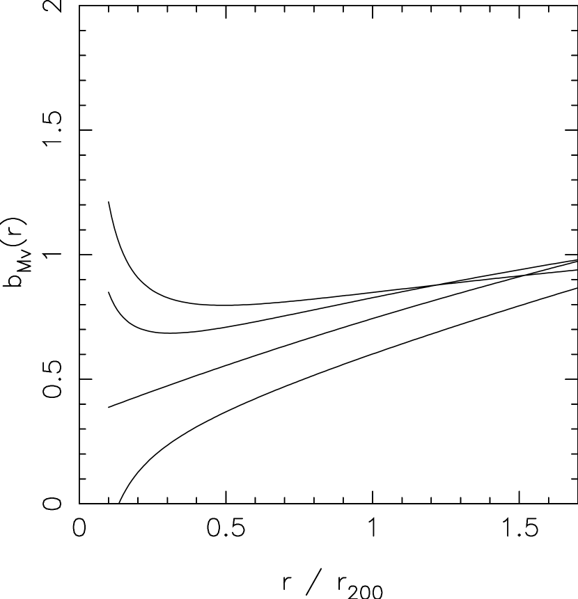
Figure 7:

Figure 8:

Figure 9:

Figure 11:

References

- Abell (1965) Abell, G. O. 1965, ARA&A, 3, 1
- Abraham et al. (1996) Abraham, R. G., Smecker-Hane, T. A., Hutchings, J. B., Carlberg, R. G., Yee, H. K. C., Ellingson, E., Morris, S., Oke, J. B., Davidge, T. 1996, ApJS, in press
- Bahcall & Tremaine (1981) Bahcall, J. & Tremaine, S. D. 1981, ApJ, 244, 805
- Barnes, Goodman & Hut (1986) Barnes, J., Goodman, J., & Hut, P. 1986, ApJ, 300, 112
- Bean et al. (1983) Bean, A. J., Efstathiou, G., Ellis, R. S., Peterson, B. A. & Shanks, T. 1983, MNRAS, 205, 605
- Beers, Flynn & Gebhardt (1990) Beers, T. C., Flynn, K. & Gebhardt, K. 1990, AJ, 100, 32
- Bertschinger (1985) Bertschinger, E. 1985, ApJS, 58, 39
- Binney & Tremaine (1987) Binney, J. & Tremaine, S. 1987, Galactic Dynamics, (Princeton University Press)
- Bird (1994) Bird, C. M. 1994, AJ, 107, 1637
- Butcher & Oemler (1984) Butcher, H. & Oemler, A. 1984, ApJ, 285, 423
- Carlberg & Dubinski (1991) Carlberg, R. G. & Dubinski, J. 1991, ApJ, 369, 13
- Carlberg (1994) Carlberg, R. G. 1994, ApJ, 433, 468
- Carlberg et al. (1994) Carlberg, R. G., Yee, H. K. C., Ellingson, E., Pritchet C., Abraham, R., Smecker-Hane, T., Bond, J. R., Couchman, H. M. P., Crabtree, D., Crampton, D., Davidge, T., Durand, D., Eales, S., Hartwick, F. D. A., Hesser, J. E., Hutchings, J. B., Kaiser, N., Mendes de Oliveira, C., Myers, S. T., Oke, J. B., Rigler, M. A., Schade, D., & West, M. 1994, JRASC, 88, 39
- C (96) Carlberg, R. G., Yee, H. K. C., Ellingson, E., Abraham, R., Gravel, P., Morris, S. M, & Pritchet, C. J. 1996a (C96), ApJ, 462, 32
- Cole & Lacey (1996) Cole, S. & Lacey, C. 1996, MNRAS, 281, 716
- Copi, Schramm & Turner (1995) Copi, C. J., Schramm, D. N., & Turner, M. S. 1995, Science, 267, 192
- Crone, Evrard & Richstone (1994) Crone, M. M., Evrard, A. E., & Richstone, D. O. 1994, ApJ, 434, 402
- Davis & Peebles (1983) Davis, M. & Peebles, P. J. E. 1983, ApJ, 267, 465
- Dekel (1994) Dekel, A. 1994, ARA&A, 32, 371
- Dekel et al. (1993) Dekel, A., Bertschinger, E., Yahil, A., Strauss, M. A., Davis, M., & Huchra, J. P. 1993, ApJ, 412, 1
- Dubinski (1993) Dubinski, J. 1993, ApJ, 401, 441
- Efron & Tibshirani (1986) Efron, B. & Tibshirani, R. 1986, Statistical Science, 1, 54
- Efstathiou, Ellis & Peterson (1988) Efstathiou, G., Ellis, R. S., & Peterson, B. A. 1988, MNRAS, 232, 431
- Fillmore & Goldreich (1984) Fillmore, J. A. & Goldreich, P. 1984, ApJ, 281, 1
- Fisher et al. (1994) Fisher, K. B., Davis, M., Strauss, M. A., Yahil, A., & Huchra, J. P. 1994, MNRAS, 267, 927
- Gioia & Luppino (1994) Gioia, I. M. & Luppino, G. A. 1994, ApJS, 94, 583
- Gioia et al. (1990) Gioia, I. M., Maccacaro, T., Schild, R. E., Wolter, Stocke, J. T., Morris, S. L., & Henry, J. P. 1990, ApJS, 72, 567
- Gott & Gunn (1972) Gott, J. R. & Gunn, J. 1972, ApJ, 176, 1
- Gott & Turner (1976) Gott, J. R. & Turner, E. L 1976, ApJ, 209, 1
- Gunn (1978) Gunn, J. E. 1978, in Observational Cosmology, eds. Maeder, A., Martinet, L, & Tammann, G. 1978 (Geneva Observatory: Sauverny)
- den Hartog (1995) den Hartog, R. 1995, The Dynamics of Rich Galaxy Clusters, Ph. D. Thesis, Leiden University
- Henry et al. (1992) Henry, J. P., Gioia, I. M., Maccacaro, T., Morris, S. L., Stocke, J. T., & Wolter, A. 1992, ApJ, 386, 408
- Hernquist (1990) Hernquist, L. 1990, ApJ, 356, 359
- Kaiser (1987) Kaiser, N. 1987, MNRAS, 227, 1
- van Kampen (1995) van Kampen, E. 1995, MNRAS, 273, 295
- Katz & White (1993) Katz, N. & White, S. D. M. 1993, ApJ, 412, 455
- Kent & Gunn (1982) Kent, S. & Gunn, J. E. 1982, AJ, 87, 945
- LeFèvre et al. (1994) LeFèvre, O., Crampton, D., Felenbok, P., & Monnet, G. 1994, A&A, 282, 340
- Limber (1959) Limber, D. N. 1959, ApJ, 130, 414
- Loveday et al. (1993) Loveday, J., Efstathiou, G., Peterson, B. A., Maddox, S. J. 1993, ApJ, 390, 338
- Merritt (1984) Merritt, D. 1984, ApJ, 313, 121
- Merritt & Tremblay (1994) Merritt, D. & Tremblay, B. 1994, AJ, 108, 514
- Mohr et al. (1995) Mohr, J. J., Evrard, A. E., Frabicant, D. G., & Geller, M. J. 1995, ApJ, 447, 8
- Navarro, Frenk & White (1995) Navarro, J. F., Frenk, C. S., & White, S. D. M. 1995, ApJ submitted
- Oort (1958) Oort, J. H. 1958, in La Structure et L’Évolution de L’Univers, Onzième Conseil de Physique, ed. R. Stoops (Solvay Institute: Bruxelles) p. 163
- Palmer & Papaloizou (1987) Palmer, P. L. & Papaloizou, J. 1987, MNRAS, 224, 1043
- Peebles (1970) Peebles, P. J. E. 1970, AJ, 75, 13
- Peebles (1993) Peebles, P. J. E. 1993, Principles of Physical Cosmology (Princeton University Press: Princeton)
- Press et al. (1992) Press, W. H., Teukolsky, S. A., Vetterling, W. T., & Flannery, B. P. 1992, Numerical Recipes in C (Cambridge University Press)
- Pryor & Geller (1984) Pryor, C. & Geller, M. J. 1984, ApJ, 278, 457
- Ramella, Geller & Huchra (1989) Ramella, M., Geller, M. J., & Huchra, J. P. 1989, ApJ, 344, 57
- Regös & Geller (1989) Regös, A. & Geller, M. J. 1989, AJ, 98, 755
- Richstone, Loeb & Turner (1992) Richstone, D. O., Loeb, A., & Turner, E. L. 1992, ApJ, 393, 477
- Richstone & Tremaine (1984) Richstone, D. O. & Tremaine, S. T. 1984, ApJ, 286, 27
- Rood et al. (1972) Rood, H. J., Page, T. L, Kintner, E. C. & King, I. R. 1972, ApJ, 175, 627
- (56) Schade, D., Carlberg, R. G., Yee, H. K. C., López-Cruz, O. & Ellingson, E. 1996a, ApJ, 464, L63
- (57) Schade, D., Carlberg, R. G., Yee, H. K. C., López-Cruz, O. & Ellingson, E. 1996b, ApJ, 465, L103
- Schwarzschild (1954) Schwarzschild, M. 1954, AJ, 59, 273
- Shaya, Peebles & Tully (1995) Shaya, E. J., Peebles, P. J. E., & Tully, R. B. 1995, ApJ, 454, 15
- Smith (1936) Smith, S. 1936, ApJ, 83, 29
- Strauss & Willick (1995) Strauss, M. A. & Willick, J. A. 1995, Phys. Rep., 261, 271
- The & White (1986) The, L. S. & White, S. D. M. 1984, AJ, 92, 1248
- Tremaine et al. (1994) Tremaine, S., Richstone, D. O., Byun, Y-I., Dressler, A., Faber, S. M., Grillmair, C., Kormendy, J., & Lauer, T. R. 1994, AJ, 107, 634
- Tsai & Buote (1995) Tsai, J. C. & Buote, D. A. 1996, ApJ, 458, 27
- van Albada (1960) van Albada, G. B. 1960, Bull. Astron. Inst. Netherlands, 15, 165
- Walker et al. (1991) Walker, T. P., Steigman, G., Kang, H., Schramm, D. M. & Olive, K. A. 1991, ApJ, 376, 51
- West & Richstone (1988) West, M. J. & Richstone, D. O. 1988, ApJ, 335, 532
- White & Fabian (1995) White, D. A. & Fabian, A. C. 1995, MNRAS, 273, 72
- White (1976) White, S. D. M. 1976, MNRAS, 177, 717
- White et al. (1993) White, S. D. M., Navarro, J. F., Evrard, A. E., & Frenk, C. S. 1993, Nature, 366, 429
- Yee, Ellingson & Carlberg (1996) Yee, H. K. C., Ellingson, E. & Carlberg, R. G. 1996, ApJS, 102, 269
- Yee et al. (1995) Yee, H. K. C., Sawicki, M. J., Ellingson, E., & Carlberg, R. G. 1995, in Fresh Views on Elliptical Galaxies ASP conference series, 86, 301
- Zembrowski & Carlberg (1996) Zembrowski, P. & Carlberg, R. G. 1996, in preparation
- Zwicky (1933) Zwicky, F. 1933, Helv. Phys. Acta 6, 110
- Zwicky (1937) Zwicky, F. 1937, ApJ, 86, 217