Adaptive Smoothed Particle Hydrodynamics: Methodology II

Abstract

Further development and additional details and tests of Adaptive Smoothed Particle Hydrodynamics (ASPH), the new version of Smoothed Particle Hydrodynamics (SPH) described in Shapiro et al. (1996; Paper I) are presented. The ASPH method replaces the isotropic smoothing algorithm of standard SPH, in which interpolation is performed with spherical kernels of radius given by a scalar smoothing length, with anisotropic smoothing involving ellipsoidal kernels and tensor smoothing lengths. In standard SPH the smoothing length for each particle represents the spatial resolution scale in the vicinity of that particle, and is typically allowed to vary in space and time so as to reflect the local value of the mean interparticle spacing. This isotropic approach is not optimal, however, in the presence of strongly anisotropic volume changes such as occur naturally in a wide range of astrophysical flows, including gravitational collapse, cosmological structure formation, cloud-cloud collisions, and radiative shocks. In such cases, the local mean interparticle spacing varies not only in time and space, but in direction as well. This problem is remedied in ASPH, where each axis of the ellipsoidal smoothing kernel for a given particle is adjusted so as to reflect the different mean interparticle spacings along different directions in the vicinity of that particle. By deforming and rotating these ellipsoidal kernels so as to follow the anisotropy of volume changes local to each particle, ASPH adapts its spatial resolution scale in time, space, and direction. This significantly improves the spatial resolving power of the method over that of standard SPH at fixed particle number per simulation.

This paper presents an alternative formulation of the ASPH algorithm for evolving anisotropic smoothing kernels, in which the geometric approach of Paper I, based upon the Lagrangian deformation of ellipsoidal fluid elements surrounding each particle, is replaced by an approach involving a local transformation of coordinates to those in which the underlying anisotropic volume changes appear to be isotropic. Using this formulation the ASPH method is presented in 2D and 3D, including a number of details not previously included in Paper I, some of which represent either advances or different choices with respect to the ASPH method detailed in Paper I. Among the advances included here are an asynchronous time-integration scheme with different time steps for different particles and the generalization of the ASPH method to 3D. In the category of different choices, the shock-tracking algorithm described in Paper I for locally adapting the artificial viscosity to restrict viscous heating just to particles encountering shocks, is not included here. Instead, we adopt a different interpolation kernel for use with the artificial viscosity, which has the effect of spatially localizing effects of the artificial viscosity. This version of the ASPH method in 2D and 3D is then applied to a series of 1D, 2D, and 3D test problems, and the results are compared to those of standard SPH applied to the same problems. These include the problem of cosmological pancake collapse, the Riemann shock tube, cylindrical and spherical Sedov blast waves, the collision of two strong shocks, and problems involving shearing disks intended to test the angular momentum conservation properties of the method. These results further support the idea that ASPH has significantly better resolving power than standard SPH for a wide range of problems, including that of cosmological structure formation.

1 Introduction

As reviewed by Monaghan (1992), the Smoothed Particle Hydrodynamics (SPH) method has proved extremely useful and versatile in simulating a wide range of astrophysical flow problems, from the formation of stars, planets, and moons, to the supernova explosions of massive stars, to the collision of stars, to the formation of galaxies and large-scale structure in cosmology, to name a few. In recent years, the SPH method, in combination with one of a variety of gravitational N-body solvers, has played a leading role in simulations of cosmological gas dynamics (e.g. Evrard 1988; Hernquist & Katz 1989, hereafter HK89; Steinmetz & Müller 1993; Navarro & White 1993; Couchman, Thomas, & Pearce 1995; Tissera, Lambas, & Abadi 1997). For such flow problems, which involve gravitational collapse, supersonic velocities, and the build-up of extremely nonlinear density and pressure contrasts, the SPH method has several advantages over traditional Eulerian finite-difference methods. As a Lagrangian method, SPH is naturally able to adjust its length resolution scale so as to follow the mass as it flows to create a highly inhomogeneous density. In addition, SPH replaces the spatial grid used in traditional finite-difference methods by an interpolation scheme based upon the smoothing of numerical data over irregularly spaced, neighboring mass points – the “particles” in SPH – thereby eliminating the problem which traditional grid-based, Lagrangian schemes have when the grid distorts too much and twists upon itself. A large body of work now exists to show that the SPH method, which is based upon the standard conservation equations of compressible gas dynamics, does indeed yield correct solutions of those equations, as long as the simulated gas is represented by a large enough number of particles, just as Eulerian finite-difference schemes yield correct solutions if the number of grid cells is large enough.

The great complexity and inhomogeneity of astrophysical flows like those studied in cosmology, however, requires an enormous number of particles (or, equivalently, grid cells in the case of Eulerian schemes) in order to resolve the multi-scale phenomena of structure formation arising from a field of Gaussian-random-noise, initial density perturbations, as typically assumed. Unfortunately, current computer hardware is inadequate to handle the required minimum number of SPH particles, in general, so some sacrifice of accuracy is inevitable. As a result, any effort to improve the accuracy and resolving power of the SPH method at fixed number of particles is extremely worthwhile. One such attempt was presented by us in Shapiro et al. (1996, hereafter Paper I), in which we replaced the isotropic smoothing algorithm of SPH, which utilizes spherical interpolation kernels characterized by a scalar smoothing length which varies in space and time according to the local variations of the gas density, by an anisotropic smoothing algorithm which uses ellipsoidal kernels characterized by a different smoothing length along each axis of the ellipsoid and varies these three axes so as to follow the value of the local mean separation of particles surrounding each particle, as it changes in time, space, and direction. A scheme was devised whereby the ellipsoidal kernels of this anisotropic smoothing algorithm were evolved continuously during a simulation so as to track the local deformations and rotations of the fluid. By analogy with the concept of adaptive mesh refinement introduced in Eulerian finite-difference methods in order to replace the traditional spatial grid with one which varies the cell size in time and space automatically so as to respond to the local need for higher spatial resolving power, we termed our modified SPH algorithm with evolving ellipsoidal kernels, “Adaptive Smoothed Particle Hydrodynamics (ASPH).”

The particular motivation for this algorithmic advance was the realization that the isotropic SPH smoothing algorithm, in which the smoothing length is traditionally adjusted in proportion to $\rho^{-1/3}$ (where $\rho$ is the gas density), is adequate for isotropic volume changes but is seriously mismatched to the generic anisotropic volume changes which occur in problems involving gravitational collapse, the collision and merging of subclumps, and strong shock waves, all common to cosmic structure formation. This problem was first discussed by Shapiro (1989) and Shapiro, Kang, & Villumsen (1991), in which the first use of anisotropic smoothing in SPH for cosmological gas dynamics was made, in order to simulate a 1D, planar, cosmological pancake collapse with a 3D, SPH code. There, the anisotropic kernels were all fixed in orientation and, for each, the axis perpendicular to the pancake plane was adjusted in proportion to $\rho^{-1}$ in order to reflect the 1D, planar geometry of collapse. The result was a significant improvement in the resolution of the pancake shocks and postshock flow compared to the traditional isotropic smoothing approach. A second problem which standard SPH has with flows like this was also noted. As had been discussed by Shapiro and Struck-Marcell (1985) before, in their 1D, Lagrangian treatment of pancake hydrodynamics, standard artificial viscosity causes gas undergoing supersonic collapse to be strongly heated, as in the pancake problem, in which gas outside the two strong shocks near the central plane, which parallel the central plane on either side, falls supersonically toward that plane. In principle, however, this heating should be restricted to gas which is actually encountering the shock. It was found to be necessary, in fact, to suppress the unphysical viscous heating of collapsing gas prior to shock formation, caused by the presence of artificial viscosity, in order to resolve the shock and postshock flow correctly. This second problem led Shapiro et al. (1996) to a second modification of SPH which Paper I describes as part of the ASPH method, that of automating the suppression of viscous heating for gas not undergoing a shock transition. In Paper I, this was accomplished by using the anisotropic kernel calculations to predict particle caustic formation as a “shock-tracking” algorithm. Only particles which were thereby identified as those in imminent danger of encountering a shock were allowed to experience artificial viscous heating. As demonstrated in detail in Paper I, the new algorithms of ASPH resulted in a substantial improvement of resolving power over the standard SPH method, at fixed particle number. The reader is referred to Paper I for the detailed demonstration of the relative shortcomings of SPH in comparison with ASPH, including several tests of ASPH, as well as a description of the algorithmic details.

The idea of using anisotropic sampling kernels with SPH dates back to Bicknell & Gingold (1983), who first utilized ellipsoidal SPH kernels in order to study the tidal flattening of stars involved in close-encounters with black holes. They exploited the special geometry of that problem, simplifying the evolution of the flattened kernel shapes. Shapiro, Martel, & Villumsen first began seriously investigating a generalized approach to the problem of using ellipsoidal sampling in SPH (Shapiro et al. 1993; Shapiro, Martel, & Villumsen 1994; Martel et al. 1994), motivated by the shortcomings noted above in SPH simulations of idealized problems typical of cosmological structure formation (i.e., the Zel’dovich pancake). This investigation ultimately led to the ASPH formulation presented in Paper I, in which the scalar smoothing length $h$ of standard SPH is generalized to a smoothing tensor ${\bf H}$, whose 9 components define three vectors ${\bf h}_{k}$ which correspond to the three axes of the smoothing ellipsoid for each particle (in 2D, the ${\bf H}$ tensor has four components, defining the axes of a smoothing ellipse). In principle, these ellipsoid axes ${\bf h}_{k}$ point along the principal axes of the local particle density distribution, with lengths proportional to the mean separation of particles along these directions. In practice, it is necessary to provide a mathematical prescription for evolving the ${\bf H}$ tensor for each particle simultaneously with the time integration of the SPH dynamical equations. In Paper I the mathematical prescription given for calculating and evolving the H tensor is a time-integration based upon the components of the deformation tensor ($\partial v_{\alpha}/\partial x_{\beta}$). A geometric approach is taken to evolve the three axes ${\bf h}_{k}$ of the smoothing ellipsoid at time $t$ into new axes at $t+\Delta t$, by treating the ellipsoid as a Lagrangian fluid element whose axes are given by ${\bf h}_{k}$ and using the tensor $\partial v_{\alpha}/\partial x_{\beta}$ explicitly to evolve the ellipsoidal fluid element. To first order in $\Delta t$ and $\Delta x$, if the surface bounding a fluid element at time $t$ is an ellipsoid, then the new surface which bounds the same fluid element after a time $\Delta t$ has elapsed must also be an ellipsoid. This approach is used explicitly to derive the evolution equations for the components of the ${\bf H}$ tensor for the case of 2D flows. The generalization of the mathematical derivation to 3D, while straightforward, was left for a future publication.

In this paper we present an alternative mathematical formalism for evolving the ASPH smoothing scale. We adopt the viewpoint that the anisotropic volume changes represented by the smoothing ellipsoid can be expressed as a local, linear transformation of coordinates to those in which the underlying anisotropic volume changes appear to be isotropic. This coordinate transformation, expressed in terms of a tensor ${\bf G}$ with units of inverse length, represents the (direction dependent) amount by which the actual interparticle distances must be rescaled in order to make the mean interparticle separations independent of direction in the transformed coordinates. The components of ${\bf G}$ are uniquely and simply related to those of the ${\bf H}$ tensor defined in Paper I, since the two prescriptions are mathematically equivalent to first-order in $\Delta t$ and $\Delta x$. In fact, the directions of the eigenvectors of ${\bf G}$ and ${\bf H}$ are identical, while the associated eigenvalues of ${\bf G}$ are the inverse of those for ${\bf H}$. Expressed in the frame in which ${\bf G}$ and ${\bf H}$ are both diagonal, that is, the diagonal elements of G are just $h_{k}^{-1}$, where $h_{k}$ are the diagonal elements of ${\bf H}$. In order to evolve ${\bf G}$ in time simultaneously with the solution of the hydrodynamical conservation equations, we evaluate ${\bf G}$ by equating the inverse square of ${\bf G}$ with a quantity similar to the inertia tensor of the smoothing ellipsoid. This yields a set of first-order differential equations for the time evolution of ${\bf G}$, once again involving the components of the deformation tensor, $\partial v_{\alpha}/\partial x_{\beta}$. The mathematical derivation for the evolution of ${\bf G}$ is valid for arbitrary dimension, and we explicitly evaluate the form of both ${\bf G}$ and its time derivative $D\mbox{${\bf G}$}/Dt$ in 2D and 3D. This represents the first time that the mathematical prescription for evolving ellipsoidal smoothing kernels has been presented explicitly in 3D.

There are a number of minor implementation differences between this work and that of Paper I. For instance, we do not use the same scheme for suppressing the artificial viscosity. The approach to the artificial viscosity presented here does not require violating energy conservation, and does not include any free parameters which are tweaked to suit a particular problem. On the downside, the algorithm presented here is not as successful at suppressing artificial viscous preheating in the Zel’dovich pancake problem as that of Paper I, though it does improve over the standard implementation of artificial viscosity used with SPH and is general in application, allowing us to test a wide variety of problems. We have also developed a number of efficient numerical algorithms in order to make ASPH applicable to large scale problems, including an adaptive asynchronous time integrator, such that each ASPH node is allowed to possess its own timestep and current time, described in detail in Appendix C. We investigate a number of test problems, including: the Zel’dovich pancake problem (to compare the formalism presented here with that of Paper I); the Sedov Blastwave solution; standard hydrodynamical tests such as the Riemann shocktube and the problem of two interacting strong shocks as described in Woodward (1982) and Woodward & Colella (1984); and a pair rotational problems designed to test the conservation of angular momentum under ASPH.

This paper is organized as follows. In §2 and §3 we describe the techniques of SPH and ASPH, deriving ASPH based upon SPH. In §4 we present various tests and comparisons of these techniques. In §5 we summarize the results of this paper and discuss directions for future work. In Appendix A we present the detailed numerical (A)SPH dynamical equations (both for proper and comoving coordinates). Appendix B presents the full mathematical formalism and derivation for defining and evolving the ASPH smoothing tensor. Finally, Appendix C outlines some of the major algorithms developed in order to efficiently implement ASPH numerically.

2 Standard SPH

ASPH is a generalization of SPH, and therefore throughout this paper we refer to “Standard” SPH as both a starting point and comparison for ASPH. Unfortunately such a standard version does not exist, as there are a variety of subtly different ways to implement SPH. Therefore in Appendix A we present the formalism for what we call Standard SPH. This discussion, in combination with what is discussed in the body of this paper, is complete, but brief. The reader who wishes a more in-depth introduction to SPH is referred to the reviews of Monaghan (1992) or Benz (1990), either of which provide an excellent introduction to this subject. For the experienced practitioner of SPH, we simply state that our implementation of SPH consists of evolving the momentum and specific thermal energy for each node based upon the Lagrangian conservation equations, accounting for pressure and gravitational forces as well as radiative cooling. The mass density is updated using the summation approach. We implement a standard Monaghan-Gingold artificial viscosity (Monaghan & Gingold 1983) defined on a pairwise basis, with the shearing correction suggested by Balsara (1995). We have derived the (A)SPH dynamical equations based upon these choices for proper time-domain coordinates, as well as comoving coordinates expressed as a function of a power of the cosmological expansion factor (for use in cosmological simulations). Finally, we allow a variable smoothing scale which evolves in accordance with the continuity equation as outlined by Benz (1990). We discuss this SPH method of evolving the smoothing scale in §3.2.

3 SPH vs. ASPH

We will now introduce the basic notation and concepts necessary to understand ASPH and how it relates to SPH. As SPH and ASPH are so similar, much of our discussion is applicable to both. In such ambiguous situations we refer to the technique as (A)SPH. The major distinction between SPH and ASPH is the manner in which smoothing scales are defined and evolved, and therefore we will concentrate on this subject. This section is organized as follows: in §3.1 we discuss how smoothing scales are defined under both SPH and ASPH, as well as how they are used in order to make interpolated estimates of local quantities; in §3.2 we discuss how a variable smoothing scale is evolved under SPH; finally in §3.3 we describe how the anisotropic smoothing of ASPH is justified and evolved. Note that we discuss ASPH descriptively here, simply presenting the resulting 2D evolution equations without their derivation. We defer a detailed discussion of the mathematics upon which ASPH is formulated until Appendix B, where the complete 2D and 3D derivations may also be found.

3.1 Interpolation under SPH & ASPH

(A)SPH functions by numerically solving the Lagrangian conservation equations at a series of discrete points or nodes, which are interrelated through an interpolation scheme. In this way (A)SPH resembles the various flavors of Lagrangian finite-difference methods, the major distinction being the method of interpolation. Under a traditional Lagrangian finite-difference approach the interpolation nodes are required to be arranged on an underlying geometry or grid, while (A)SPH’s interpolation scheme makes no such restrictions.

Under the SPH formalism, the interpolated value of a quantity $F$ at some spatial position ${\bf r}$ is defined through the integral

$$\mbox{$\left\langle F({\bf r})\right\rangle$}=\int F({\bf r}^{\prime})W({\bf r}-{\bf r}^{\prime},h)\,d{\bf r}^{\prime}.$$ (1)

The function $W({\bf r},h)$ is called the interpolation kernel, where $h$ represents the SPH smoothing scale. The interpolation kernel has the properties

$$\int W({\bf r}-{\bf r}^{\prime},h)\,d{\bf r}^{\prime}=1,$$ (2)

$$\lim_{h\to 0}W({\bf r}-{\bf r}^{\prime},h)=\delta({\bf r}-{\bf r}^{\prime}).$$ (3)

Note from equation (3) that although the integration of equation (1) formally extends over all space, in fact the most important contributions to the integral occur within a few $h$ of the position ${\bf r}$. This reflects the localized nature of hydrodynamic interactions.

In SPH applications, $h$ is defined as a scalar quantity associated with each discrete SPH node. Thus, SPH interpolation about any given node using such a scalar smoothing scale is isotropic in nature. In other words, each SPH node samples a spherical volume about itself, regardless of the physical conditions in which it is embedded. As we discuss in §3.3, in general this is not optimal. In order to implement an anisotropic smoothing scheme, we require a more generalized methodology for defining smoothing scales. We begin by noting that the interpolation kernel can be written as a function of $\mbox{\boldmath$\eta$}\equiv{\bf r}/h$, such that we can restate $W({\bf r},h)=W({\bf r}/h)=W(\mbox{\boldmath$\eta$})$. In general we refer to $\eta$ as the normalized position vector.

We can now introduce a generalized method of mapping from real to normalized position space (${\bf r}\to\mbox{\boldmath$\eta$}$), which we define through a linear transformation ${\bf G}$. In comparison with SPH, this relation is

SPH: $\mbox{\boldmath$\eta$}={\bf r}/h\quad\to\quad$ ASPH: $\mbox{\boldmath$\eta$}=\mbox{${\bf G}$}{\bf r}$.

Clearly the ${\bf G}$ tensor has the units of an inverse length-scale. The simplest generalization of the spherical smoothing implemented by SPH is to allow smoothing in elliptical (2D) or ellipsoidal (3D) volumes. Placing such a restriction upon ${\bf G}$ implies that it must be a real, symmetric matrix. Our scheme under ASPH then is to associate such an ellipsoidal ${\bf G}$ tensor with each computational node, taking the place of the scalar smoothing scale $h$ of SPH. Under this formalism, SPH can be thought of as a special case of ASPH, where the ${\bf G}$ tensor is diagonal and each diagonal element is equal to $1/h$.

Under this notation it is simple to define an ASPH kernel estimate. We need only replace the SPH method of defining $\eta$ with the ASPH method in the kernel function $W(\mbox{\boldmath$\eta$})=W(\mbox{${\bf G}$}{\bf r})$. However, we also require the spatial gradient of the interpolation kernel $\mbox{${\bf\nabla}$}W$ in order to implement the (A)SPH dynamical equations. This can be expressed through equation (4), so long as we are neglecting ${\bf\nabla}$${\bf G}$ terms (an important assumption we will return to in §3.4)

$$\mbox{${\bf\nabla}$}W(\mbox{${\bf G}$}{\bf r})=\frac{\partial W(\mbox{${\bf G}$}{\bf r})}{\partial{\bf r}}=\frac{\partial\mbox{\boldmath$\eta$}}{\partial{\bf r}}\frac{\partial W}{\partial\mbox{\boldmath$\eta$}}=\mbox{${\bf G}$}\frac{\mbox{\boldmath$\eta$}}{\eta}\frac{\partial W}{\partial\eta}.$$ (4)

Before we can go on to express how to use ${\bf G}$ in making kernel interpolations, we must deal with how to symmetrize such estimates. This issue arises for SPH with a variable smoothing scale as well. The problem can be understood by examining equation (1), which expresses the interpolated value of some general quantity $F$ in terms of a volume integral involving $h$. This equation makes no mention of how to deal with a smoothing scale which varies spatially $h({\bf r})$. One could choose to either use $h({\bf r})$ (known as a “gather” formalism) or $h({\bf r}^{\prime})$ (“scatter”). However, it is advantageous to spatially symmetrize the kernel estimation process such that $W({\bf r},{\bf r}^{\prime},h({\bf r}),h({\bf r}^{\prime}))=W({\bf r}^{\prime},{\bf r},h({\bf r}^{\prime}),h({\bf r}))$ in order to symmetrize the (A)SPH dynamical equations, thereby ensuring rigorous conservation of quantities such as linear momentum. In order to accomplish this we adapt the symmetrization scheme of Hernquist & Katz (HK89), which defines a symmetrized kernel estimate as the average of both the gather and scatter approaches. In terms of two discrete positions ${\bf r}_{i}$ and ${\bf r}_{j}$, the symmetrized kernel function W_ij is

$$\mbox{W${}_{ij}$}\equiv\frac{1}{2}\left[W(\mbox{\boldmath$\eta$}_{i})+W(\mbox{\boldmath$\eta$}_{j})\right],$$ (5)

where

$$\mbox{\boldmath$\eta$}_{i}\equiv\mbox{${\bf G}$}_{i}\mbox{${\bf r}_{ij}$},\quad\mbox{\boldmath$\eta$}_{j}\equiv\mbox{${\bf G}$}_{j}\mbox{${\bf r}_{ij}$},$$ (6)

$$\mbox{${\bf r}_{ij}$}\equiv{\bf r}_{i}-{\bf r}_{j}.$$ (7)

A symmetrized gradient of the kernel can be similarly defined as

$$\mbox{$\mbox{${\bf\nabla}$}\mbox{W}_{ij}$}\equiv\frac{1}{2}\left[\mbox{${\bf\nabla}$}W(\mbox{\boldmath$\eta$}_{i})+\mbox{${\bf\nabla}$}W(\mbox{\boldmath$\eta$}_{j})\right].$$ (8)

These forms also arise naturally from a derivation of (A)SPH based upon the variational principle.

The interpolation relation of equation (1) can now be represented numerically by assigning known values for the general quantity $F({\bf r})$ on a series of discrete nodes at positions ${\bf r}_{j}$ (each with an associated mass $m_{j}$, mass density $\rho_{j}$, and number density $n_{j}=\rho_{j}/m_{j}$), such that we have a discrete set $F_{j}$. The interpolated value of $F$ at position ${\bf r}_{i}$ is

$$F_{i}\equiv\mbox{$\left\langle F({\bf r}_{i})\right\rangle$}=\sum_{j}\frac{F_{j}}{n_{j}}\mbox{W${}_{ij}$}=\sum_{j}F_{j}\frac{m_{j}}{\rho_{j}}\mbox{W${}_{ij}$}.$$ (9)

Note that equation (9) basically represents a monte-carlo interpretation of equation (1). With this machinery in place, it is now possible to derive ASPH dynamical equations using the same approach as SPH. So long as we use the notational conventions outlined above (expressing quantities in terms of the normalized position vector $\eta$ rather than explicitly using $h$) the SPH and ASPH dynamical equations are identical. We present our complete set of (A)SPH dynamical equations derived in this fashion in Appendix A.

The form of the ${\bf G}$ tensor depends upon the dimensionality in which it implemented. The ${\bf G}$ tensor can be defined in terms of the underlying geometry as follows. In 2D, consider a unit normalized position isocontour associated with a given ${\bf G}$. In general such an isocontour represents an arbitrary ellipse in real position space, which is uniquely defined by a semi-major axis $h_{1}$, semi-minor axis $h_{2}$, and position angle $\psi$ associated with the semi-major axis. Since we are considering a unit isocontour, $h_{1}$ and $h_{2}$ are the smoothing scales along the primary axes of the ellipse. In terms of these geometrical quantities, the elements of the ${\bf G}$ tensor are (see Appendix B)

$$\mbox{${\bf G}$}=\left(\begin{array}[]{cc}G_{11}&G_{21}\\ G_{21}&G_{22}\end{array}\right)=\left(\begin{array}[]{cc}\mbox{$h_{1}^{-1}$}\cos^{2}\psi+\mbox{$h_{2}^{-1}$}\sin^{2}\psi&(\mbox{$h_{1}^{-1}$}-\mbox{$h_{2}^{-1}$})\cos\psi\sin\psi\\ (\mbox{$h_{1}^{-1}$}-\mbox{$h_{2}^{-1}$})\cos\psi\sin\psi&\mbox{$h_{1}^{-1}$}\sin^{2}\psi+\mbox{$h_{2}^{-1}$}\cos^{2}\psi\end{array}\right).$$ (10)

The 3D ${\bf G}$ tensor can be similarly derived, as discussed in appendix B.4, resulting in equation (B35).

We have discussed the interpolation kernel $W$ completely generally to this point. There are many possible choices for such a function, so long as the criteria of equations (2) and (3) are met and they can be expressed as functions of the normalized position $\eta$. The most popular forms currently in use with SPH are the Bi-Cubic Spline and the Gaussian kernels. In our investigation we use the Bi-Cubic Spline, which in $\nu$ dimension is

$$\mbox{$W^{\nu\mbox{\scriptsize-D}}_{\mbox{\scriptsize spline}}$}(\mbox{\boldmath$\eta$})=\mbox{$A^{\nu\mbox{\scriptsize-D}}_{\mbox{\scriptsize spline}}$}\left\{\begin{array}[]{l@{\quad}l}1-3/2\,\eta^{2}+3/4\,\eta^{3},&0\leq\eta\leq 1;\\ 1/4\,(2-\eta)^{3},&1<\eta\leq 2;\\ 0,&\eta>2,\end{array}\right.$$ (11)

$$\mbox{${\bf\nabla}$}\mbox{$W^{\nu\mbox{\scriptsize-D}}_{\mbox{\scriptsize spline}}$}(\mbox{\boldmath$\eta$})=\mbox{$A^{\nu\mbox{\scriptsize-D}}_{\mbox{\scriptsize spline}}$}\mbox{${\bf G}$}\frac{\mbox{\boldmath$\eta$}}{\eta}\left\{\begin{array}[]{l@{\quad}l}-3\eta+9/4\,\eta^{2},&0\leq\eta\leq 1;\\ -3/4\,(2-\eta)^{2},&1<\eta\leq 2;\\ 0,&\eta>2,\end{array}\right.$$ (12)

$$\mbox{$A^{1\mbox{\scriptsize-D}}_{\mbox{\scriptsize spline}}$}=\frac{2}{3}|\mbox{${\bf G}$}|,\quad\mbox{$A^{2\mbox{\scriptsize-D}}_{\mbox{\scriptsize spline}}$}=\frac{10}{7\pi}|\mbox{${\bf G}$}|,\quad\mbox{$A^{3\mbox{\scriptsize-D}}_{\mbox{\scriptsize spline}}$}=\frac{1}{\pi}|\mbox{${\bf G}$}|,$$ (13)

where $A^{\nu\mbox{\scriptsize-D}}_{\mbox{\scriptsize spline}}$ represents the normalization constant required to meet the condition of equation (2).

3.2 Evolving the Smoothing Scale under SPH

Before going on to discuss how ${\bf G}$ is evolved under ASPH, we must begin with the rationale for evolving the variable smoothing scale under SPH. Most modern implementations of SPH allow an individual, time variable smoothing scale to be associated with each SPH node, such that $h({\bf r},t)$. The justification for implementing and evolving such a variable smoothing scale is based upon the philosophy that each SPH node should sample roughly the same number of “significant neighbors” (that is, the number of neighboring SPH nodes within some critical threshold distance, usually expressed as a multiple of the smoothing scale $\eta\leq\mbox{$\eta^{\mbox{\scriptsize cut}}$}$). This implies that each SPH node will always sample roughly the same amount of mass, which is consistent with SPH’s Lagrangian nature. This results in higher resolutions in dense regions, while still maintaining meaningful (if poorly resolved) measurements in low density regions. This condition can be stated mathematically in $\nu$ dimensions as $h_{i}\propto\rho_{i}^{-1/\nu}$ for a given node $i$.

A well-defined standard method for evolving the SPH smoothing scale in order to meet this criterion is based upon the continuity equation (Benz 1990 and references therein), and can be expressed as

$$\frac{Dh_{i}}{Dt}=-\frac{1}{\nu}\frac{h_{i}}{\rho_{i}}\frac{D\rho_{i}}{Dt}=\frac{h_{i}}{\nu}(\mbox{${\bf\nabla}$}\cdot{\bf v})_{i}=-\frac{1}{\nu}\frac{h_{i}}{\rho_{i}}\sum_{j}m_{j}\mbox{${\bf v}_{ij}$}\cdot\mbox{$\mbox{${\bf\nabla}$}\mbox{W}_{ij}$}.$$ (14)

3.3 Evolving ${\bf G}$ under ASPH

In order to understand the motivation for developing ASPH, it is necessary to understand the potential inefficiencies of the SPH approach as defined by equation (14). Consider a system undergoing planar collapse in some arbitrary direction. In 3D, the standard SPH smoothing scale will adapt to this collapse process as $h\propto\rho^{-1/3}$. However, a purely planar collapse is really a 1D problem, and ideally smoothing scales perpendicular to the plane of collapse should evolve as $h_{\bot}\propto\rho^{-1}$, while smoothing scales parallel to the collapse should remain unchanged. In such a situation, the approach in 3D SPH will lead to less than optimal resolution along the direction of collapse (since $h_{\bot}$ is shrinking too slowly), while nodes in the collapsing region will lose contact with neighbors parallel to the collapse (since $h_{\|}$ is shrinking, but the internode spacing parallel to the plane of collapse remains unchanged). In general, problems of computational interest are not isotropic in nature, and in particular gravitational clustering scenarios generically result in strongly anisotropic density evolution. ASPH seeks to address this problem by allowing an anisotropic definition of the smoothing process, as well as a self-consistent method for evolving this anisotropic smoothing function. The ASPH algorithm can be viewed as trying to adapt to the physical or intrinsic dimensionality of a problem, rather than the imposed geometrical dimensionality.

This line of reasoning suggests a straightforward approach to evolving the ASPH smoothing transformation ${\bf G}$. We can generalize the SPH philosophy of attempting to maintain the same number of neighbors per node into an attempt to maintain the same number of neighbors in all directions for each node. This can be rephrased to state that we will try to keep the distribution of neighboring nodes isotropic in normalized ($\eta$) space. In more physical terms each ASPH node attempts to always sample the same Lagrangian volume as the system evolves, which is appropriate for ASPH’s Lagrangian nature. This can be viewed as an attempt to track the local deformation of a fluid element with an idealized shape corresponding to the underlying geometry of the ${\bf G}$ tensor. At best such a picture represents an analogy, as a true fluid element is not constrained to remain ellipsoidal, and the volumes defined by the collection of $\mbox{${\bf G}$}_{i}$’s interpenetrate. Nevertheless, the fluid element analogy is useful in order to gain an intuitive sense as to the behaviour of the ${\bf G}$ tensors.

The deformation tensor $\sigma$ ($\sigma_{\alpha\beta}\equiv\partial v_{\alpha}/\partial r_{\beta}$ where $(\alpha,\beta)$ refer to spatial directions) indicates how the velocity field varies spatially to first-order, such that ${\bf v}({\bf r}+d{\bf r})\approx{\bf v}({\bf r})+\mbox{\boldmath$\sigma$}~{}d{\bf r}$. This quantity predicts how a local volume of the fluid will deform with time. If we visualize the ASPH interpolation volume as an embedded volume within the fluid, $\sigma$ predicts how this volume should be deformed by the local velocity field, such that the enclosed Lagrangian volume remains constant. As this is a first-order transformation, an initially ellipsoidal volume will be in general be mapped to a new ellipsoidal volume, guaranteeing that our ellipsoidal transformation for ${\bf G}$ will remain appropriate. Under the (A)SPH formalism the deformation tensor can be estimated by

$$\mbox{$\left\langle\sigma_{\alpha\beta}\right\rangle$}_{i}=-\sum_{j}m_{j}(v_{ij})_{\alpha}\frac{\partial\mbox{W${}_{ij}$}}{\partial r_{\beta}}.$$ (15)

We will defer a rigorous mathematical derivation of ${\bf G}$ and its evolution to appendix B, and simply present the results for the 2D case here. The evolution of the 2D ${\bf G}$ tensor (eq. [10]) is given by

$$\frac{D\mbox{${\bf G}$}}{Dt} = \left(\begin{array}[]{cc}DG_{11}/Dt&DG_{21}/Dt\\ DG_{21}/Dt&DG_{22}/Dt\end{array}\right)$$ (18)

$$= \left(\begin{array}[]{cc}G_{21}(\dot{\theta}-\sigma_{21})-G_{11}\sigma_{11}&G_{22}\dot{\theta}-G_{11}\sigma_{12}-G_{21}\sigma_{22}\\ -G_{11}\dot{\theta}-G_{21}\sigma_{11}-G_{22}\sigma_{21}&-G_{21}(\dot{\theta}+\sigma_{12})-G_{22}\sigma_{22}\end{array}\right),$$ (21)

$$\dot{\theta} = \frac{G_{11}\sigma_{12}-G_{22}\sigma_{21}-G_{21}(\sigma_{11}-\sigma_{22})}{G_{11}+G_{22}}.$$ (22)

In order to demonstrate the connection of this evolution equation for ${\bf G}$ with the SPH relation for $h$, consider the evolution of the determinant $|\mbox{${\bf G}$}|$.

$$\frac{D|\mbox{${\bf G}$}|}{Dt} = G_{11}\frac{DG_{22}}{Dt}+G_{22}\frac{DG_{11}}{Dt}-2G_{21}\frac{DG_{21}}{Dt}$$

$$= -(G_{11}G_{22}-G_{21}^{2})(\sigma_{11}+\sigma_{22})$$

$$= -|\mbox{${\bf G}$}|\mbox{${\bf\nabla}$}\cdot{\bf v}$$

$$= \frac{|\mbox{${\bf G}$}|}{\rho}\frac{D\rho}{Dt}.$$

For the special case of SPH, the determinant reduces to $\mbox{$|\mbox{${\bf G}$}|^{\mbox{\scriptsize SPH}}$}=h^{-\nu}$ in $\nu$ dimensions. In 2D, the SPH evolution equation for $h$ (eq. [14]) yields

$$\frac{Dh^{-2}}{Dt}=-2h^{-3}\frac{Dh}{Dt}=\frac{h^{-2}}{\rho}\frac{D\rho}{Dt}.$$ (24)

Equation (3.3) shows that $|\mbox{${\bf G}$}|$ is directly proportional to the density $(|\mbox{${\bf G}$}|\propto\rho)$. This also proves that the smoothing volume represented by $|\mbox{${\bf G}$}|^{-1}$ under ASPH evolves identically with its SPH counterpart, demonstrating that for the case of isotropic evolution ASPH formally reduces to SPH. Though derived here in 2D, this result applies in general.

3.4 Stabilizing ASPH: Smoothing the ${\bf G}$ Tensor Field

The evolution equation for the ${\bf G}$ tensor is derived based upon first-order arguments about the local velocity field – specifically, that the local velocity can be approximated by ${\bf v}({\bf r}+d{\bf r})\approx{\bf v}({\bf r})+\mbox{\boldmath$\sigma$}~{}d{\bf r}$. Clearly, in complex simulations one can encounter situations where this approximation is not valid on “local” scales (scales of order a few $h$). A cosmological example of such a situation is the formation of a poorly resolved cluster at the intersection of several filaments, each of which contains gas streaming into the cluster. Ideally one would wish to resolve all mass scales adequately such that the “local” velocity field will always be well represented by $\sigma$ on scales of $h$, but in reality computational limitations make this infeasible. Any simulation will always have a lower mass cutoff in the resolved mass distribution. In particular, a Cold Dark Matter like initial density fluctuation power-spectrum will generically have substantial power on small scales, and it is reasonable to assume that in such situations one will have to deal with nonlinear velocity fields down to scales of $h$.

If we examine the assumptions underlying our derivation of the evolution equations for ${\bf G}$, we find that we implicitly require the ${\bf G}$ tensor field to be well-behaved on scales of a few smoothing lengths. This point can be demonstrated in two ways. First, consider the expression for the gradient of the kernel $\mbox{${\bf\nabla}$}W$ (eq. [4]). As with SPH, we neglect any ${\bf\nabla}$${\bf G}$ terms, which formally should be included. Including these terms is somewhat problematic as they must be estimated numerically, and we have found that attempting to include them does little more than introduce noise. Neglecting such terms implies that we require ${\bf\nabla}$${\bf G}$ to be negligible on scales of a few characteristic smoothing lengths. Another way of viewing this problem emerges if we use our idealized fluid element analogy. The smoothing volumes represented by neighboring ${\bf G}$ tensors must necessarily overlap – this implies that the ${\bf G}$ tensors of closely neighboring nodes should represent the same local idealized fluid element. Strong disorder in this ${\bf G}$ tensor field on local scales is therefore inconsistent.

Arguments such as these lead us to conclude that we require the ${\bf G}$ tensor field to be almost uniform on scales of a few smoothing lengths, and smoothly varying on larger scales. If this condition is not met, how would we expect this inconsistency to affect ASPH? Under our standard formulation of SPH, it will formally conserve mass (with the summation definition for the density), linear and angular momentum (because all pair interactions are symmetric and radial), while energy is conserved to second-order. ASPH utilizes the same dynamical equations as SPH, including the use of the symmetrized kernel function W_ij (eq. [5]). Therefore, ASPH will rigorously conserve mass and linear momentum, while energy will be conserved to second-order (see Appendix A for a discussion of the dynamical equations and these conservation properties). However, because the gradient of the kernel $\mbox{${\bf\nabla}$}W$ is not necessarily radial under ASPH, forces between interacting pairs of nodes will not in general be radial and therefore angular momentum will not be rigorously conserved. This makes the conservation of angular momentum under ASPH analogous to the conservation of energy – angular momentum will only be conserved to the order that the system is being solved (in general to second-order). ASPH is therefore vulnerable to errors in the angular momentum as well as the energy, and we might expect that as an ASPH simulation breaks down non-conservation of these quantities could be a symptom. As we discuss in §4.2, we find precisely this sort of behaviour.

We therefore require a method of ensuring that the ${\bf G}$ tensor field is well-behaved. The most obvious step to take is to smooth the ${\bf G}$ tensor field using the ASPH formalism. We must be cautious in the implementation of such a scheme, however. Recall that the ${\bf G}$ tensor has units of an inverse smoothing scale. Taking a straight ASPH estimate of ${\bf G}$ is equivalent to taking the harmonic mean of the smoothing scales, which can be unstable toward small smoothing scales. Additionally, we would like to preserve the property of the determinant $|\mbox{${\bf G}$}|$ such that it evolves smoothly in accordance with the local density, as demonstrated in equation (3.3). Discontinuous changes in ${\bf G}$ are equivalent to discontinuously changing an individual nodes contribution to the local density. After exploring several possible implementations for a smoothing scheme, we have settled on the following approach. Periodically each $\mbox{${\bf G}$}_{i}$ tensor is replaced by an averaged $\mbox{${\bf G}$}_{i}^{\prime}$ calculated as

$$\mbox{$\left\langle\mbox{${\bf G}$}^{-1}\right\rangle$}_{i}=\frac{\sum_{j}\mbox{${\bf G}$}_{j}^{-1}\mbox{W${}_{ij}$}}{\sum_{j}\mbox{W${}_{ij}$}},\quad\mbox{${\bf G}$}_{i}^{\prime}=|\mbox{${\bf G}$}_{i}|\,\left|\mbox{$\left\langle\mbox{${\bf G}$}^{-1}\right\rangle$}_{i}\right|\mbox{$\left\langle\mbox{${\bf G}$}^{-1}\right\rangle$}_{i}^{-1}.$$ (25)

Note this scheme represents three modifications of an ordinary ASPH average. First, we average the quantity $\mbox{${\bf G}$}^{-1}$ in order to avoid the problems of a harmonic mean on the smoothing scale. Second, we force the determinant to be preserved $|\mbox{${\bf G}$}_{i}^{\prime}|=|\mbox{${\bf G}$}_{i}|$. Finally, we force the normalization of the average to be unity by dividing by $\sum_{j}\mbox{W${}_{ij}$}$. Formally this sum should be unity (eq. [2]), but in practice because we only sum over a finite number of nodes, this quantity typically deviates from that ideal. We have found that normalizing the average in this way increases the stability of the technique. The frequency with which we must enforce this smoothing process must be determined experimentally. We have found that smoothing roughly once or twice every characteristic timescale is generally adequate (where by characteristic timescale we mean the timescale setting the current timestep – see appendix C.2).

It is worth noting that there is an alternate method of viewing this problem and its solution. The evolution of the ${\bf G}$ tensor is based upon attempting to follow the deformation of the local velocity field based on using the deformation tensor $\sigma_{\alpha\beta}=\partial v_{\alpha}/\partial x_{\beta}$, which is only correct to a first-order. If the local velocity field is not this obligingly simple, then the arguments we base our ${\bf G}$ evolution equations on break down and there is no guarantee trouble will not ensue. This leads to the idea that smoothing on the deformation tensor $\left\langle\mbox{\boldmath$\sigma$}\right\rangle$ could also be an equivalent method of dealing with this problem. Such a solution seems intuitively pleasing, as it would no longer involve directly fiddling with the ${\bf G}$ tensors themselves. However, this is basically equivalent to our adopted method of smoothing on the ${\bf G}$ tensors, which has the additional advantage of directly guaranteeing the good behaviour of the ${\bf G}$ tensor field. We should also point out that formally SPH also requires that $\mbox{${\bf\nabla}$}h$ be negligible on scales of a few $h$, and therefore standard SPH schemes utilizing a spatially variable smoothing scale should also ensure this behaviour in some way. Steinmetz & Müller (1993) find that the stability of SPH with a variable smoothing scale is indeed improved by spatially smoothing the $h$ field.

3.5 Artificial Viscosity under ASPH

Cosmological simulations often show evidence of nonphysical preheating in shock forming regions, particularly during collapse situations. This can result in poor resolution of shockfronts and related phenomena. This behaviour is due to the use of an artificial viscosity such as that denoted by $\Pi$ in the (A)SPH dynamical equations [A.1] & [A.1]). Such an artificial viscosity term is required in the (A)SPH formalism both for stability and because without it (A)SPH is insufficiently dissipative to prevent the interpenetration of converging streams of gas, resulting in a poor representation of shock conditions. However, the artificial viscosity is by definition an artificial term, and ideally its use should be restricted solely to ongoing shocks, where it is required. This problem is particularly accentuated in cosmological studies, since the kinetic energy is typically much larger than the thermal, and the artificial viscosity functions by converting kinetic to thermal energy. Inspection of the standard Monaghan-Gingold (1983) form of the artificial viscosity (eqs. [A11] & [A12]) shows that traditionally $\Pi$ is restricted to only be active for convergent flows within the material being modeled. While a convergent flow is a minimal requirement for the presence of shocks, clearly not all convergent flows necessarily result in the formation of shocks (e.g. homologous collapse). This overuse of $\Pi$ is what leads to the excessive heating of the material around shockfronts, a problem which can be especially troublesome in gravitational collapse scenarios, where the spurious preheating of the gas can become acute enough to interfere with the collapse process itself. As this is precisely the sort of scenario we are concerned with modeling well, we would like to improve upon this algorithm.

This line of reasoning led to the development of the algorithm outlined in Paper I for the suppression of the artificial viscosity. Through experimentation we determined that it is possible to delay the turn-on time for the artificial viscosity in the energy equation (which is the source of the spurious heating), but it is necessary to keep the artificial viscosity active in the momentum equation in order to prevent interpenetration of the (A)SPH nodes. That scheme yields excellent results insofar as suppressing the artificial viscous preheating of material, particularly in the Zel’dovich pancake scenario, for which it was developed. In this paper we adopt a different prescription for suppressing the artificial viscosity. Rather than attempting to delay the turn-on time for $\Pi$ and treating it distinctly between the momentum and energy equations, we instead adopt a different interpolation kernel to be used with $\Pi$, which we denote as W${}^{\Pi}_{ij}$. We choose a form for W${}^{\Pi}_{ij}$ such that it is more spatially compact and has a sharper gradient than W_ij. We use the standard artificial viscosity turn-on criteria (given in eq. [A11]), and make no distinction between $\Pi$ in the momentum and energy equations. In effect, this approach can be thought of as restricting the influence of the artificial viscosity spatially, rather than temporally as the scheme of Paper I.

There are many possible choices that could be used for W${}^{\Pi}_{ij}$. In order to successfully suppress the preheating problem while still stopping interpenetration, we want a kernel which is more spatially compact and possesses a stronger gradient as compared with the Spline kernel (eq. [11]). We use a simple variant of the Gaussian kernel, as given by

$$\mbox{$W^{\nu\mbox{\scriptsize-D}}_{\mbox{\scriptsize Gauss2}}$}(\mbox{\boldmath$\eta$})=\mbox{$A^{\nu\mbox{\scriptsize-D}}_{\mbox{\scriptsize Gauss2}}$}\exp\left(-K\eta^{4}\right),$$ (26)

where the appropriate normalization constants are

$$\mbox{$A^{1\mbox{\scriptsize-D}}_{\mbox{\scriptsize Gauss2}}$}=\frac{2K^{1/4}|\mbox{${\bf G}$}|}{\Gamma(1/4)},\quad\mbox{$A^{2\mbox{\scriptsize-D}}_{\mbox{\scriptsize Gauss2}}$}=\frac{2K^{1/2}|\mbox{${\bf G}$}|}{\pi^{3/2}},\quad\mbox{$A^{3\mbox{\scriptsize-D}}_{\mbox{\scriptsize Gauss2}}$}=\frac{K^{3/4}|\mbox{${\bf G}$}|}{\pi\Gamma(3/4)}.$$ (27)

The gradient of this kernel is

$$\mbox{${\bf\nabla}$}\mbox{$W^{\nu\mbox{\scriptsize-D}}_{\mbox{\scriptsize Gauss2}}$}(\mbox{\boldmath$\eta$})=\mbox{${\bf G}$}\frac{\mbox{\boldmath$\eta$}}{\eta}\frac{\partial\mbox{$W^{\nu\mbox{\scriptsize-D}}_{\mbox{\scriptsize Gauss2}}$}}{\partial\eta}=-4K\mbox{$W^{\nu\mbox{\scriptsize-D}}_{\mbox{\scriptsize Gauss2}}$}\eta^{2}\mbox{${\bf G}$}\mbox{\boldmath$\eta$}.$$ (28)

Through experimentation we have found setting $K=1.5^{4}$ is a safe choice. Using this kernel as W${}^{\Pi}_{ij}$ successfully prevents interpenetration in all of our test cases, while still reducing the preheating of the ASPH gas in collapse simulations (see the Zel’dovich pancake tests in §4.1.1). Comparison of these results with similar 2D pancake runs in Paper I reveal that this form of $\Pi$ suppression is not as effective as that presented in Paper I, at least for this class of problems. However, this scheme does have the advantages that it is applicable in all situations (there are no problem dependent parameters to fiddle), and because $\Pi$ is treated identically in the momentum and energy equations energy conservation is preserved.

Finally, we should point out that while we find using this modified artificial viscosity works well under the ASPH tests presented in this paper, we also find in similar SPH experiments that it has little effect when used in conjunction with SPH. The precise reason for this remains unclear, but it is possible that the planar shocks in these problems are simply not well enough resolved in the SPH models we perform. One could therefore infer if the SPH resolution were improved by using a larger number of particles, we might ultimately find some benefit to this scheme under SPH.

4 Tests

In this section we discuss a set of test cases performed under both ASPH and SPH. These tests have been selected to compare the relative advantages of the two techniques, as well as to test questions about the validity of ASPH (in particular the angular momentum issue). We concentrate on 2D simulations, for the pragmatic reason that we must run problems in at least 2D for there to be a distinction between ASPH and SPH (in 1D the two are formally identical), while 3D simulations are much more computationally expensive. We present a few low-resolution 3D versions of some of our tests, to begin exploring the validity of the technique in 3D. We defer extensive testing of the 3D formalism for now. All simulation results presented as SPH utilize our “Standard” SPH formalism, outlined in Appendix A. All ASPH simulations have been performed using both smoothing of the ${\bf G}$ tensor field (§3.4) and special treatment of the artificial viscosity (§3.5), unless otherwise noted. In appendix C we present a brief discussion of the specific algorithms used to perform these simulations.

We present two broad classes of test cases: those which are physically 1D (such as the Zel’dovich pancake problem, the Sedov Blastwave, and a few flavors of the Riemann Shocktube), and those which are physically 2D (rotating tests such as the Pseudo-Keplerian Disk and a collapsing disk with angular momentum).

4.1 1D Test Cases

This class of test problems, although performed in higher dimensional frameworks, possess symmetries which allow them to considered physically 1D. These tests are chosen for two reasons. First, they possess analytical solutions, allowing objective comparison and judgment of the results. Secondly, since they are physically 1D they represent cases where ASPH can be expected to have an advantage over SPH, in that ASPH can recognize and adapt to the physical dimensionality of the problem, whereas SPH cannot. We present four examples of this class of problem: the Zel’dovich pancake (§4.1.1), the Sedov blastwave (§4.1.2), a simple 4:1 Riemann shocktube (§4.1.3), and a double-shocktube with two interacting strong shockfronts (§4.1.4). The first two cases are chosen to typify the sorts of problems we are interested in solving as well as demonstrating the distinction between ASPH and SPH, while the last two represent standard hydrodynamic test cases.

4.1.1 Zel’dovich Pancake Test

This class of problems consists of setting up 1D plane-wave perturbations in an arbitrary dimension cosmological scenario (Zel’dovich 1970), and has been well-studied previously in scenarios which incorporate gas dynamics as well as collisionless dark matter (Shapiro & Struck-Marcell 1985). The Zel’dovich problem represents a standard test case for cosmological codes (Efstathiou et al. 1985; Villumsen 1989). As this class of problems has been discussed extensively in Paper I as well as Shapiro & Struck-Marcell (1985), we need not go over the analytical properties here. We reexamine this problem primarily because the implementation of ASPH used for this work differs from that of Paper I, and because here we present 3D as well as 2D results. Pancake collapse represents a simplified example of the sort of cosmological structure formation scenarios we wish to investigate in general.

All of the Zel’dovich Pancake simulations we present are performed under an Einstein-de Sitter cosmology ($\Omega=1$, $\Lambda=0$), with equal baryonic and dark matter mass fractions ($\Omega^{\mbox{\scriptsize bary}}$ = $\Omega^{\mbox{\scriptsize dm}}$ = 0.5). The baryonic gas is assumed to be a pure hydrogen, adiabatic gas ($\mu=1$, $\gamma=5/3$). Since these simulations are carried out in a cosmological framework, they are evolved in comoving coordinates using a power of the expansion factor ($p=a^{\alpha}$), rather than time, as the integration variable (see appendix A.2). The system is simulated in a periodic unit volume, using a 2D Particle-Mesh (PM) gravity calculation to solve for the self-gravitation. We present 2D examples and a low-resolution 3D example of this problem. In 2D, the gravity obeys a $1/r$ force law, such that each pair of nodes interact gravitationally as though they are a pair of infinite, thin, parallel rods in 3D. In this way the 2D simulations can be thought of as a “slice” through an infinite 3D simulation. Table 1 summarizes the major simulation parameters we use for our Zel’dovich pancake simulations.

Under this framework, we present ASPH and SPH simulations of 2D Zel’dovich pancakes with $(k_{x}=0,k_{y}=1)$ and $(k_{x}=2,k_{y}=1)$, and a 3D version with $(k_{x}=0,k_{y}=0,k_{z}=1)$. All ${\bf G}$ tensors are initialized as SPH spherical tensors with the determinant $|\mbox{${\bf G}$}|$ scaled appropriately for the local density. This is somewhat inconsistent for ASPH runs, since the linear evolution of an ASPH ${\bf G}$ tensor should only affect the geometry of the ${\bf G}$ tensors perpendicularly to the plane of collapse. However, at $a=1$ the initial conditions are almost uniform (the perturbations are small), and starting in this manner allows both the SPH and ASPH runs to use identical initial conditions.

Single-Wavelength 2D Zel’dovich Pancakes:

This case represents the simplest possible class of this problem: a single-wavelength pancake along one principal axis. Here we choose to use $(k_{x}=0,k_{y}=1)$, which corresponds to a collapse proceeding in the $y$ direction – by symmetry, there should be no evolution in the $x$ direction.

Figure 1: “Kernel plots” ($h=0.2$ smoothing scale isocontours) for the central region in the $(k_{x}=0,k_{y}=1)$ 2D Zel’dovich pancake simulations. The upper and lower panels on the left show the ASPH simulation at expansions $a/a_{c}=1.5$ and $a/a_{c}=2.5$, respectively, while the right-hand panels show the SPH simulation at the same times.

Figure 1 gives examples of what we refer to as “kernel plots”. These are plots of smoothing scale isocontours about each (A)SPH node in a given region. In 2D, SPH kernel plots are circles about each nodes position, whereas in general ASPH kernel plots are ellipses. We generically choose to plot the $h=0.2$ isocontour. Since the spline kernel extends to a cutoff radius of $\mbox{$\eta^{\mbox{\scriptsize cut}}$}=2$, this implies each node “sees” neighbors out to a contour 10 times that shown. We find that these sorts of figures are quite useful in order to gain an intuitive feel for how the ${\bf G}$ tensor field is adapting to the local fluid flow. In this case, we have plotted subregions centered about the pancake midplane at expansion factors $a/a_{c}=1.5$ and $a/a_{c}=2.5$. We can see that ASPH is better able to deal with this sort of 1D flow, since the ASPH ${\bf G}$ tensors can adapt the smoothing scales fully in the $y$ direction, whereas SPH must adapt smoothing scales isotropically. In other words, the ASPH smoothing scale in the $y$ direction is better able to evolve as the ideal $\rho^{-1}$ (since the collapse is a 1D process), whereas the SPH smoothing scales are constrained to evolve as $\rho^{-1/2}$. This implies not only that ASPH is better able to sample along the physically interesting dimension where the collapse is occurring, but also avoids the undesirable effect of losing neighbor information parallel to the plane of the pancake. Since the SPH smoothing scale must shrink isotropically as each node falls into the pancake, while the internode spacing parallel to the pancake is not changing, communication between the nodes parallel to the pancake begins to break down. This makes SPH more unstable to perturbations in the $x$ direction, as is evident in the SPH kernel plot at $a/a_{c}=2.5$ (the bottom right panel in Figure 1). This disorder in the SPH node positions is purely a hydrodynamical problem, since the dark matter does not suffer from such deviations. In the ASPH plots we can also see that, while formally there should be no evolution of the ASPH smoothing scale parallel to the pancake plane, this quantity is changing slightly. This is due to the fact that we preserve the determinant $|\mbox{${\bf G}$}|$ when we smooth the ${\bf G}$ tensor field. Without such smoothing, the ASPH ${\bf G}$ tensors do not demonstrate any evolution parallel to the pancake plane.

Figure 2: Half-wavelength profiles of density $\rho$, specific thermal energy $u$, velocity $v$, and pressure $P$ as a function of distance from the pancake caustic $d_{c}$ for the $(k_{x}=0,k_{y}=1)$ 2D Zel’dovich pancake simulations. All quantities are converted to proper coordinates and are expressed in units of the critical density, pancake wavelength, and the Hubble time at the beginning of the simulation. The solid lines are the analytical expectations, the square points ASPH results, and the crossed points SPH. The left panel is at $a/a_{c}=1.5$, while the right shows $a/a_{c}=2.5$.

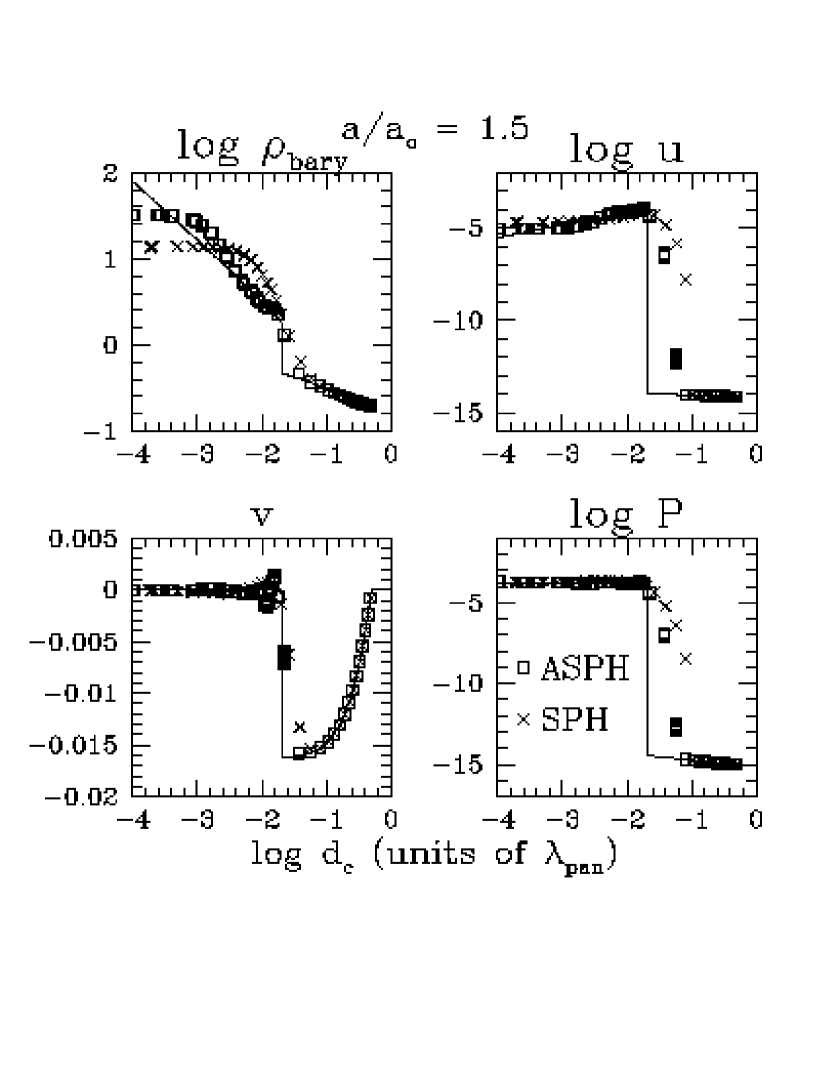
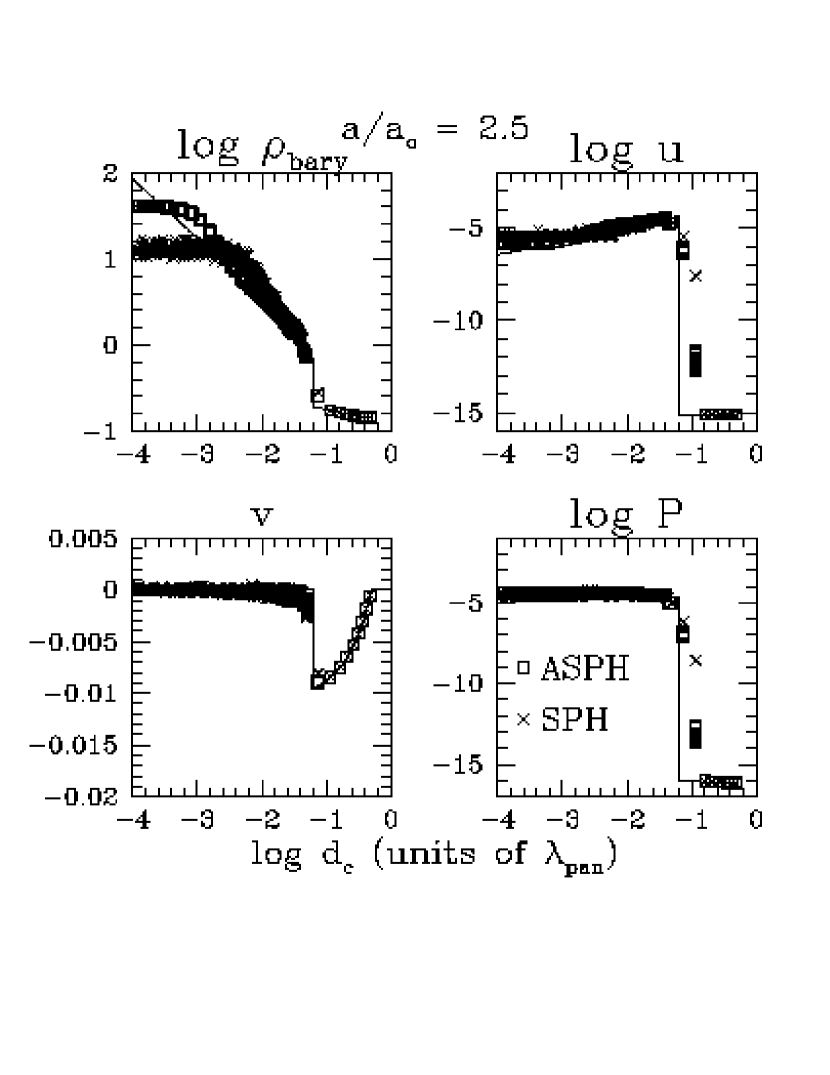
Figure 2 shows half-wavelength profiles for the mass density $\rho$, specific thermal energy $u$, velocity $v$, and pressure $P$ for the baryonic component of these simulations, plotted as a function of distance from the pancake caustic $d_{c}$. This figure represents the system for $y\geq 0.5$, and can be thought of as looking parallel to the pancake in the $x$ direction through the system. Since there are $64^{2}$ (A)SPH nodes in these simulations, there are effectively 64 nodes per wavelength (since this is a physically 1D problem), or 32 nodes per half-wavelength as plotted here. Bear in mind that all nodes in the region $y\geq 0.5$ are plotted, and therefore each of the “points” seen actually represents 64 overlapping points which share the same $x$ coordinate. It is clear where the symmetry in these simulations breaks down, as these points begin to diverge. This symmetry breaking is particularly evident in the final results at $a/a_{c}=2.5$ in the SPH simulation. ASPH’s finer resolution along the direction of collapse allows a better representation of the physical state of the system. In particular, ASPH resolves peak densities in the plane of collapse $\sim 3$ times what SPH is capable of with the same number of nodes. Additionally, ASPH proves much more stable against symmetry breaking than SPH, since the ASPH nodes are able to sample effectively parallel to the pancake even under extreme collapse. The careful reader will note, however, that the gravitational softening due to the PM grid becomes important for scales below $\log d_{c}/\mbox{$\lambda_{\mbox{\scriptsize pan}}$}\lesssim-2.1$, and the scales where we reach our peak densities ($\log d_{c}/\mbox{$\lambda_{\mbox{\scriptsize pan}}$}\sim-3$ in the ASPH case) are below this threshold. The scales at which the shock transitions themselves occur are certainly resolved by the expansions considered here, but just how far in the results can be trusted is somewhat unclear. For this problem the gravitational softening does not necessarily represent the scale at which numerics begins to dominate the solution, because the trajectories of the mass elements are essentially ballistic as they approach the pancake caustic, and therefore the gravitational acceleration at that point is of secondary importance. This conclusion is supported by the fact these profiles are unchanged when the models are rerun with four times as many PM gridcells ($256^{2}$ rather than $128^{2}$), and therefore twice the linear gravitational resolution.

Figure 3: Evolution of the global energies (kinetic, thermal, potential, and Layzer-Irvine sum) for the $(k_{x}=0,k_{y}=1)$ 2D Zel’dovich pancake simulations.

Figure 3 plots the evolution of the global energies (kinetic, thermal, potential, and the Layzer-Irvine sum) throughout these simulations. The Layzer-Irvine energy sum, $L.I.=a^{4}(K.E.+T.E.)+a\Phi-\int\Phi\,da$ (Efstathiou et al. 1985), demonstrates that both ASPH and SPH conserve global energy equivalently, with fluctuations in this total of less than a percent the total fluctuation in its components.

A natural question which might arise at this point is: how many particles would an SPH simulation require to treat this problem roughly as well as ASPH? We could, for instance, choose to match the maximum resolved density, which differs by about a factor of 3. The SPH smoothing scale is related to the density and total number of particles as $\mbox{$h_{\mbox{\scriptsize SPH}}$}\propto\rho^{-1/\nu}\propto N^{-1/\nu}$ in $\nu$ dimensions, implying that the resolved density varies linearly with the number of particles. We can therefore estimate that an SPH simulation would require of order 3 times as many particles in order to resolve the peak density equivalently to ASPH in this problem. The ASPH algorithm itself (e.g., using and evolving the ${\bf G}$ tensors) involves very little computational penalty compared with straight SPH – the majority of the increased computational effort is due the smaller timesteps required by ASPH’s increased resolution. Since an SPH simulation with equivalent resolution would also require such smaller timesteps, the overall computational penalty for running an SPH simulation with equivalent resolution to our ASPH example is roughly given by the increased number of particles, or again roughly a factor of 3 in this case. Alternately, if we instead choose to try and match the maximum linear resolution achieved, experiments such as those shown in Paper I indicate SPH would require of order 10 times as many particles per dimension to match ASPH, implying 100 times as many particles in 2D or 1000 times in 3D.

However, it is important to consider these sorts of comparisons with caution, as the results depend upon both the problem in question and precisely what it is we are trying to match. Because both ASPH and SPH are Lagrangian techniques their intrinsic resolutions are most naturally expressed in terms of a mass resolution, fundamentally represented by the discretization of the mass in the simulation into particles. The actual mass resolution achieved is a convolution of the particle mass scale with the local (A)SPH interpolation kernel, which is where the spatial adaptability of the technique comes into play. The theoretical ideal mass resolution is set by the particle discretization, and the degree to which this resolution is actually realized at each point in a problem is determined by how well the local spatial filtering adapts to the distorting particle distribution, making this a complicated, problem dependent question. All the comparisons in this paper relate SPH and ASPH experiments using the same number of particles and the same number of neighbors per particle, and therefore formally have the same ultimate limiting mass resolution. We can improve the fidelity of the SPH runs by using more particles until the quantitative SPH results for some chosen parameter (such as the peak density for a particular structure) match those of ASPH. However, by increasing the number of particles we are in fact using an SPH experiment with a potentially much better mass resolution than the ASPH example. The results of such intrinsically unbalanced comparisons can be misleading. As an example, consider the collapse of a planar perturbation such as the Zel’dovich pancake. Suppose this pancake is subject to some instability which causes it to depart from planar symmetry after the pancake shocks form, leading to the formation of clumps and filaments in the postshock layer. Suppose the mass of the clumps which are physically produced by this instability is too small to be resolved by either the SPH or ASPH simulations when they have the same particle number, because that mass is below the mean mass per smoothing volume, for example. In that case, one would not expect to see the production of the clumps in either method. If one were to try to offset the poorer spatial resolving power of the SPH method at the same particle number as the ASPH method, by increasing the particle number of the SPH method by some substantial factor, however, then the nominal mass resolution of the SPH method increases as well. It might then be possible for the SPH method to produce clumps as expected from the existence of the instability, while the ASPH simulation with fewer particles resolves the pancake shocks just as well but is not capable of producing transverse clumping. In this example we would find qualitatively different results because we have fundamentally altered the underlying resolution of the experiment, and are therefore probing different physical regimes.

These sorts of problem dependent, confusing comparisons can be avoided by recognizing that the fundamental resolution of these techniques is best expressed as a mass per smoothing volume, or more precisely as the mass per smoothing scale within each representative volume. ASPH is better able to maintain a fixed mass per smoothing scale in the presence of evolving physical anisotropies than SPH, and thereby strives to better and more consistently realize the theoretical mass resolution set by the particle discretization throughout the computational volume, regardless of how the particle distribution is distorted. A more appropriate way to compare the two techniques is that, for physically anisotropic situations such as demonstrated here, ASPH allows a more effective representation of the underlying physics than an SPH model for a given number of particles at relatively little computational penalty. The distinction is not unlike that of comparing SPH with a variable smoothing scale to the case with constant smoothing: the resolution of SPH with a constant smoothing scale depends on how many particles happen to fall within a given smoothing volume at any point during the problem; SPH with variable smoothing improves upon this by trying to ensure that each particle samples the same amount of mass at all times; ASPH goes further still in that it tries to ensure that at all times each particle will sample the same amount of mass in every direction, so that the mass per smoothing scale is held constant. ASPH is not a substitute for improving the fundamental mass resolution through increasing the number of particles, but rather strives to maintain the best possible realization of the ideal Lagrangian resolution for a given number of particles.

We should also point out that comparison of the profiles for the Zel’dovich pancake shown here with analogous figures in Paper I demonstrates that, while the results are fundamentally the same (i.e., the relative improvement offered by ASPH over SPH), the shock transition is more tightly constrained using the formalism of Paper I. This distinction is due to the difference in the methods used to suppress the artificial viscosity. The method described in Paper I is clearly more effective at capturing the sharp shock transition in this problem.

Multiple-Wavelength 2D Zel’dovich pancakes:

Figure 4: Kernel plots for the multiple-wavelength $(k_{x}=2,k_{y}=1)$ 2D Zel’dovich pancake simulations @ $a/a_{c}=2.5$. The left panel shows the ASPH run, and the right SPH.

Figure 5: Half-wavelength physical profiles of density $\rho$, specific thermal energy $u$, velocity $v$, and pressure $P$ as a function of distance from the pancake caustic $d_{c}$ for the $(k_{x}=2,k_{y}=1)$ 2D Zel’dovich pancake simulations. Units and plotting conventions are the same as used in Figure 2. The left panel shows results for $a/a_{c}=1.5$, and the right shows $a/a_{c}=2.5$.

Figure 6: Evolution of the global energies (kinetic, thermal, potential, and Layzer-Irvine sum) for the multiple-wavelength $(k_{x}=2,k_{y}=1)$ 2D Zel’dovich pancake simulations.

We now present a slightly modified pancaking problem: that of $(k_{x}=2,k_{y}=1)$. In this case there are $5^{1/2}$ wavelengths in our computational volume, each tilted with respect to the principal axes. This problem represents no fundamental change from the previous example, but rather provides an example where the physical problem does not align with any special simulation symmetry (i.e., there is no alignment with either a simulation axis or any special direction with respect to the initial node seeding). The only real difference between this and the previous single-wavelength example is that now the resolution per wavelength is effectively reduced, since we have increased the number of waves in the box with the same number of particles. There are now effectively $64/5^{1/2}\sim 28$ nodes per wavelength, or $\sim 14$ nodes per half-wavelength.

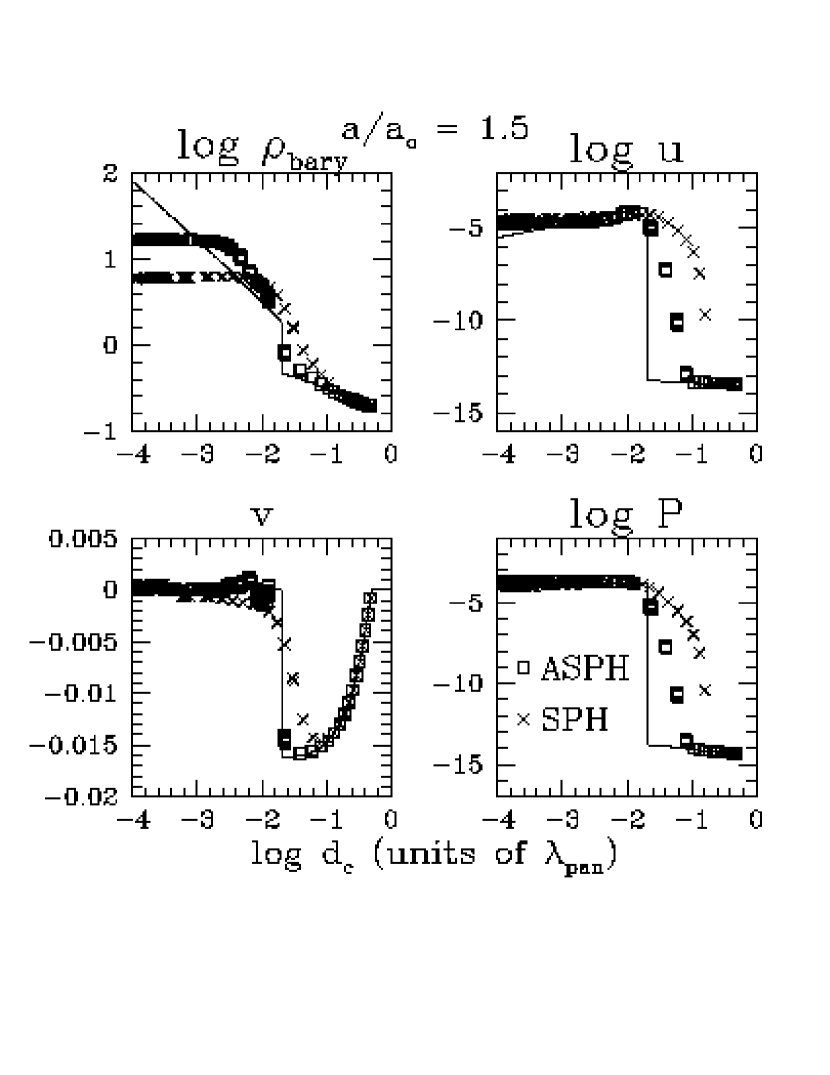
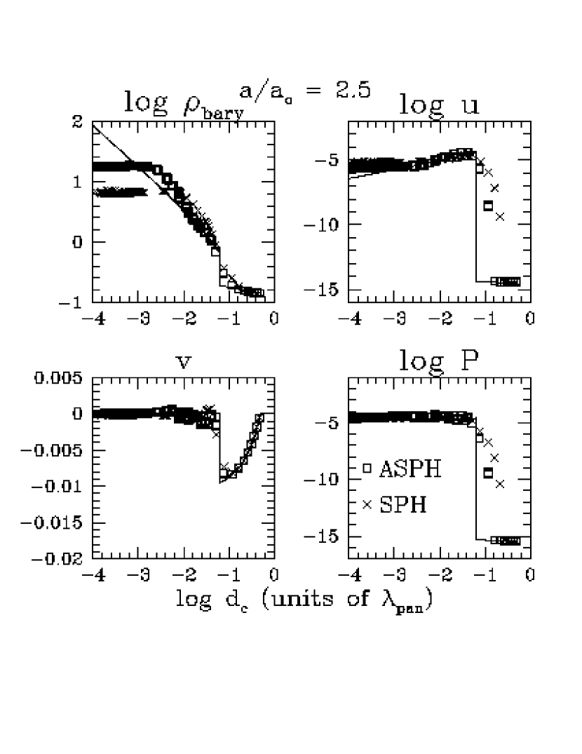
Figure 4 presents kernel plots for both the SPH and ASPH simulations at expansion $a/a_{c}=2.5$. It is clear that ASPH has successfully adapted to the tilted geometry of this problem. Additionally, there is no evidence of the transverse perturbations evident in the single-wavelength case (as is particularly notable for SPH at $a/a_{c}=2.5$). This difference is due to the fact that in the $(k_{x}=0,k_{y}=1)$ case we are trying to stack up nodes exactly one on top of the other. Any deviation from this perfect line-up will be amplified, and lead to a breakdown in the symmetry. In the $(k_{x}=2,k_{y}=1)$ case we have broken that symmetry, and therefore the instability is greatly reduced. Figure 5 presents half-wavelength profiles for both simulations at expansion factors $a/a_{c}=1.5$ and $a/a_{c}=2.5$. The results are fundamentally the same as shown in Figure 2 – ASPH again resolves central densities $\sim 3$ times those in the equivalent SPH experiment. We can therefore conclude that it would take SPH 3 times as many particles (and CPU work) to produce equivalent fidelity for this problem, though with the same caveats as outlined for such comparisons in §4.1.1. Finally, Figure 6 shows the evolution of the global energies for these simulations. Again there is little qualitative change from the single-wavelength case, with a total energy conservation violation of less than a percent.

Single-Wavelength 3D Zel’dovich Pancakes:

Figure 7: Kernel plots for 3D Zel’dovich pancake simulations @ $a/a_{c}=2.5$. We only display a thin slice $(x\in[0.4,0.6],y\in[0.50.52],z\in[0.4,0.6])$ out of unit volume simulations, rotated slightly for clarity. The $h=0.2$ isocontours are drawn as wire-mesh surfaces. The left panel shows the ASPH simulation, and the right SPH.

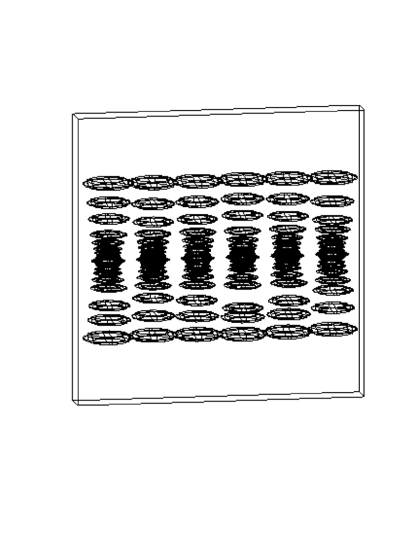
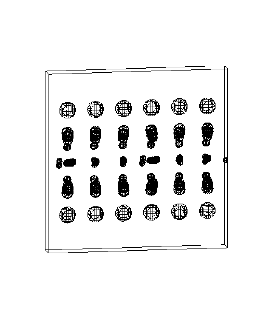
We now revisit the single wavelength version of the problem in 3D with $(k_{x}=0,k_{y}=0,k_{z}=1)$. These 3D simulations are much lower resolution than the 2D cases – with only $32^{3}$ nodes in 3D as compared with $64^{2}$ in 2D, we have effectively lowered the spatial resolution by a factor of two and the mass resolution by a factor of 8. In Figure 7 we present kernel plots of an ASPH and an SPH simulation at $a/a_{c}=2.5$. For clarity we have selected out only a single plane of nodes in the central regions of the simulation to display. The surfaces are again $h=0.2$ isocontours – note that in general ASPH kernels are ellipsoidal in shape, while SPH are spherical. It is evident that ASPH retains the ability to recognize and adapt to the 1D nature of this collapse, flattening out the kernels as they fall into the pancake caustic. The SPH kernels, which are restricted to remain spherical, are not able to adapt as well to the ongoing collapse. By $a/a_{c}=2.5$, it is clear that the SPH simulation is breaking the symmetry of the problem, as the SPH nodes begin to slip by one another and become disorganized in the pancake midplane. The ASPH simulation maintains the physical symmetry of the problem more effectively.

Figure 8: Half-wavelength profiles of density $\rho$, specific thermal energy $u$, velocity $v$, and pressure $P$ as a function of distance from the pancake caustic $d_{c}$ for the $(k_{x}=0,k_{y}=0,k_{z}=1)$ 3D Zel’dovich pancake simulations at $a/a_{c}=2.5$. All quantities are converted to proper coordinates and are expressed in units of the critical density, pancake wavelength, and the Hubble time at the beginning of the simulation. Solid lines represent the analytical expectations. The left-hand panel shows the ASPH simulation, and the right SPH.

Figure 9: Evolution of the global energies (kinetic, thermal, potential, and Layzer-Irvine sum) for the $(k_{x}=0,k_{y}=0,k_{z}=1)$ 3D Zel’dovich pancake simulations.

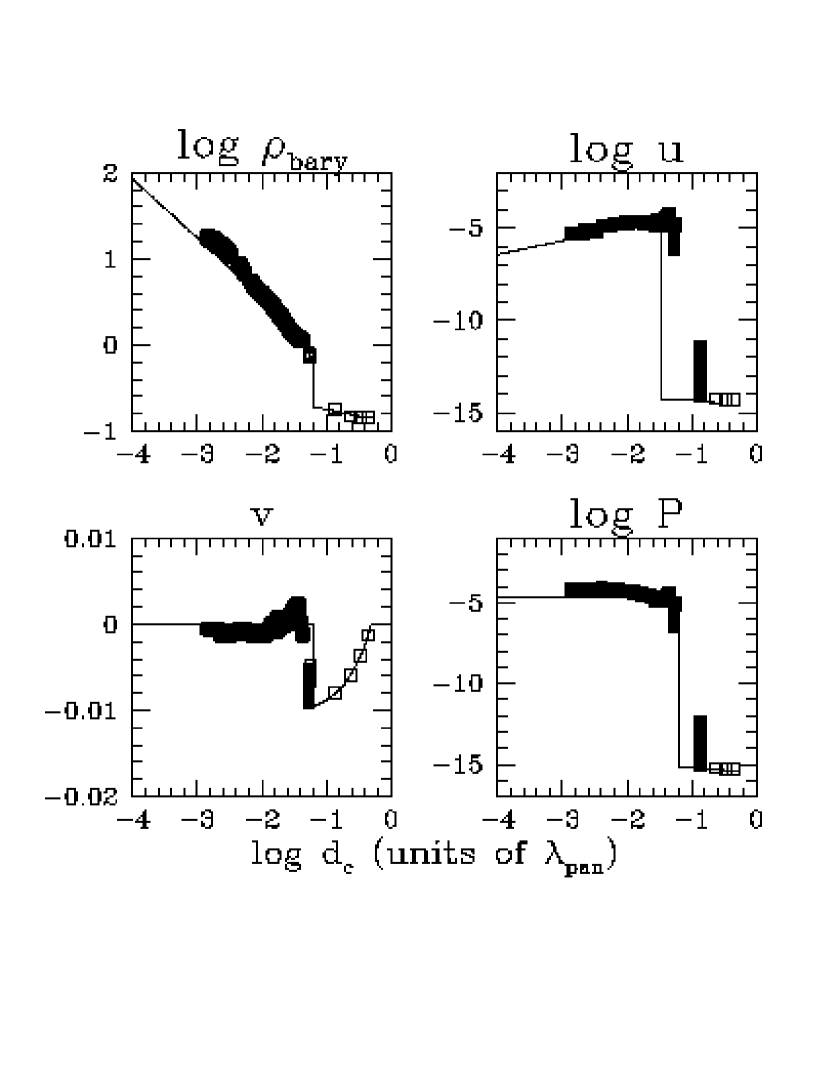
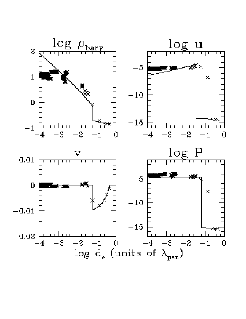
We can see the physical effects of these differences in the profiles presented in Figure 8. Comparing the density profiles at $a/a_{c}=2.5$, the ASPH simulation follows the analytical profile essentially as far the nodes can resolve (down to scales $d_{c}/\mbox{$\lambda_{\mbox{\scriptsize pan}}$}\sim 10^{-3}$), whereas the SPH simulation fails to on scales of $d_{c}/\mbox{$\lambda_{\mbox{\scriptsize pan}}$}\sim 10^{-2}$, becoming quite disordered on smaller scales. At all times the shock transition is both more sharply defined and better localized under ASPH. Finally in Figure 9 we present the evolution of the global energies throughout these 3D simulations. As in 2D, we find that both techniques conserve energy to better than 1%.

4.1.2 Sedov Blastwave Test

We will now turn to an entirely different class of test problems: that of an intense explosion in a gas. This problem possesses a set of well-known similarity solutions (Sedov 1959). We simulate this problem in both 2D and 3D, and compare the results to Sedov’s solutions in the appropriate geometry. This problem represents a somewhat difficult case for Lagrangian techniques such as (A)SPH, since the void is dynamically important.

The formal initial condition for this problem is to introduce an intense point source of thermal energy into an initially pressureless, homogeneous gas. This immediately poses a problem for any (A)SPH formalism, as (A)SPH cannot represent a discontinuous energy distribution. Therefore, in order to initialize this problem we distribute a thermal energy spike amongst a small number of nodes in the gas, and then smooth this distribution. This results in an energy spike in the gas resembling the shape of our smoothing kernel, as this is the closest (A)SPH can come to representing a delta function. The remaining nodes are initialized with a small, but finite, internal energy in order to simulate an initially pressureless gas. All ${\bf G}$ tensors are initialized as identical, spherical SPH tensors appropriate for the undisturbed initial density $\rho_{0}$ and desired number of significant neighbors per smoothing length $N_{h}$. The major simulation parameters we use for our Sedov blastwave simulations are summarized in Table 2.

2D Sedov Blastwave Simulations:

Figure 10: Kernel plots for 2D Sedov blastwave simulations at time $t=0.12$ for the cases of ASPH (left panel) and SPH (right panel).

Figure 11: Surface plots of the mass density field $\rho$ in one quadrant of the expanding shockfront for the 2D Sedov blastwave simulations at $t=0.12$. The left panel shows the ASPH simulation, and the right SPH.

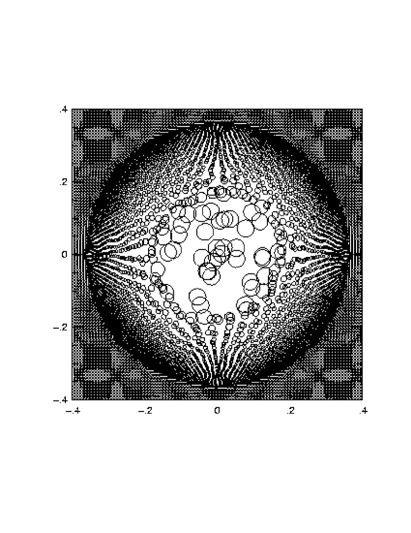
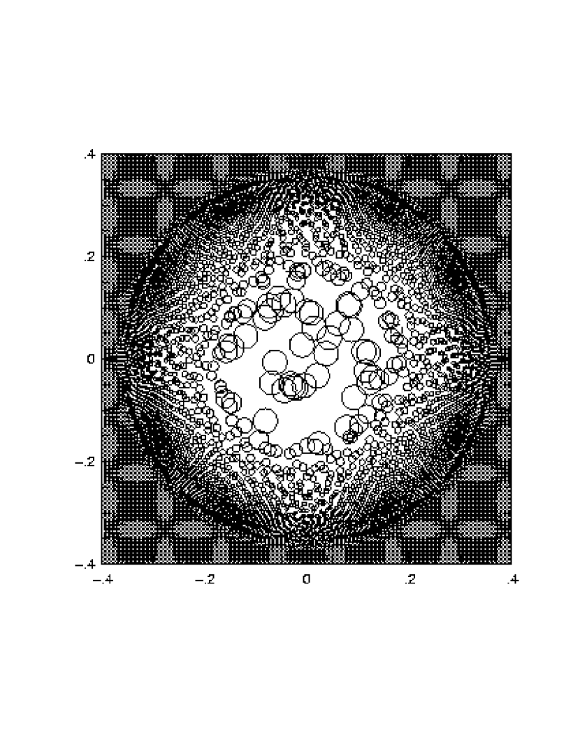
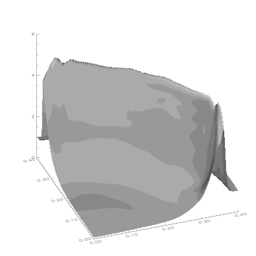
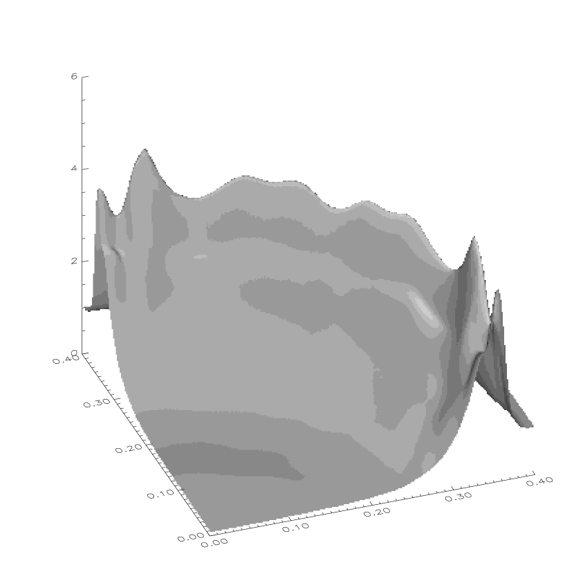
Figure 10 presents kernel plots for an ASPH and an SPH simulation of this problem at time $t=0.12$. It is clear that the ASPH model is more successful at producing a round, azimuthally symmetric shockfront than the SPH case. ASPH is able to produce a better shape for the shock because the ASPH smoothing scale parallel to the shockfront is not shrinking, and therefore communication between the nodes parallel to the shockfront is maintained. The effects of this difference are evident in Figure 11, which shows surface plots of the density in one quadrant of the blast for each of these runs. It is clear that the SPH density along the shock front shows greater fluctuations compared with the ASPH runs, which maintains the most consistent symmetry.

Figure 12: Azimuthally averaged radial density profiles for ASPH (open squares) and SPH (crosses) simulations of the 2D Sedov blastwave at times $t$ = 0.04, 0.08, 0.12, and 0.16. The SPH simulation is offset radially for clarity – the ASPH curves show the correct radial position. Each point represents the average of a radial bin containing 100 nodes. The solid lines show the analytic, cylindrical Sedov solution.

Figure 13: Azimuthally averaged radial profiles of mass density $\rho(r)$, pressure $P(r)$, and radial velocity $v_{r}(r)$ for the 2D Sedov blastwave simulations at time $t=0.12$. Shown are ASPH (open squares), SPH (crosses), and the cylindrical Sedov solution (solid lines). Each point represents an average for a radial bin containing 100 nodes.

Figure 12 presents a time-series of azimuthally averaged radial density profiles for these simulations, binned in radial steps of equal numbers of particles. Shown are times in the interval $t\in[0.02,0.16]$. The SPH run has been offset radially for clarity. Since we use $\gamma=1.4$, the strong-shock prediction for the density jump at the shock front is $\rho_{2}/\rho_{1}=(\gamma+1)/(\gamma-1)=6$. The ASPH runs converge to a peak shock density $\rho_{2}>5$ fairly rapidly, while the SPH run does not achieve a similar peak density until the end of the simulation, by which time the shock has swept up most of the particles in the simulation. The reason for these differences is that the ASPH ${\bf G}$ tensors are able to adapt to the radial nature of the problem, allowing the radial smoothing scale to adjust much more readily than SPH’s isotropic approach allows. We can gauge how well ASPH’s anisotropic smoothing is adapting to the predicted density jump by examining how elliptical the kernels are becoming. For the predicted density jump of $\rho_{2}/\rho_{1}=6$, we would expect the ratio of the shortest to longest axis of an ASPH node in the shock front to be $6^{-1}\sim 0.167$, while we in fact find in the simulation $h_{2}/h_{1}\sim 0.145$ at the shock front. It is heartening that, as expected, the SPH results converge with the ASPH as the number of nodes increases. It should be noted, however, that even though the SPH radial profiles do eventually catch up with ASPH, SPH never achieves as round a shockfront. Figure 13 presents radial profiles of the radial velocity $v_{r}$, mass density $\rho$, and pressure $P$ at $t=0.12$. Also plotted is the cylindrical Sedov solution, as the solid lines. The break in the pressure profile at $r\sim 0.2$ lies between the mass elements which mark the edge of the initial thermal energy spike.

Figure 14: Evolution of the global energies (kinetic, thermal, and total) for the 2D Sedov blastwave simulations.

Finally, Figure 14 presents the evolution of the global energies for 2D Sedov models. During the ASPH run the total energy fluctuates peak to peak $\Delta E/E\sim 2\%$ the fluctuation of its components, while SPH only suffers fluctuations of $\Delta E/E\sim 0.2\%$. It is not unexpected for ASPH to have slightly worse energy conservation than SPH, because ASPH introduces more degrees of freedom into the problem. The difference is analogous to comparing SPH with a fixed smoothing scale to SPH with variable smoothing.

3D Sedov Blastwave Simulations:

We also examine 3D simulations of the Sedov blastwave problem under both ASPH and SPH. In this case we use $N=32^{3}$ (A)SPH nodes, which results in a linear resolution of only one quarter what we have in 2D. We can therefore expect the 3D simulations to be much lower-resolution than the previous 2D case.

Figure 15: Kernel plots for 3D Sedov blastwave simulations at time $t=0.1$ for the cases of ASPH (left panel) and SPH (right panel). These figures show a small slice through the expanding blastwave for clarity: the region plotted is $(x\in[0,0.45],y\in[0,0.45],z\in[0,0.02])$ out of a unit volume.

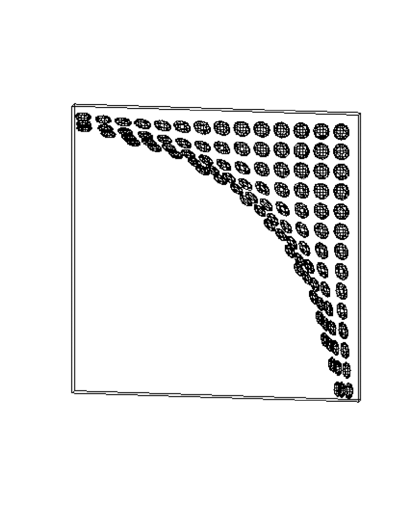
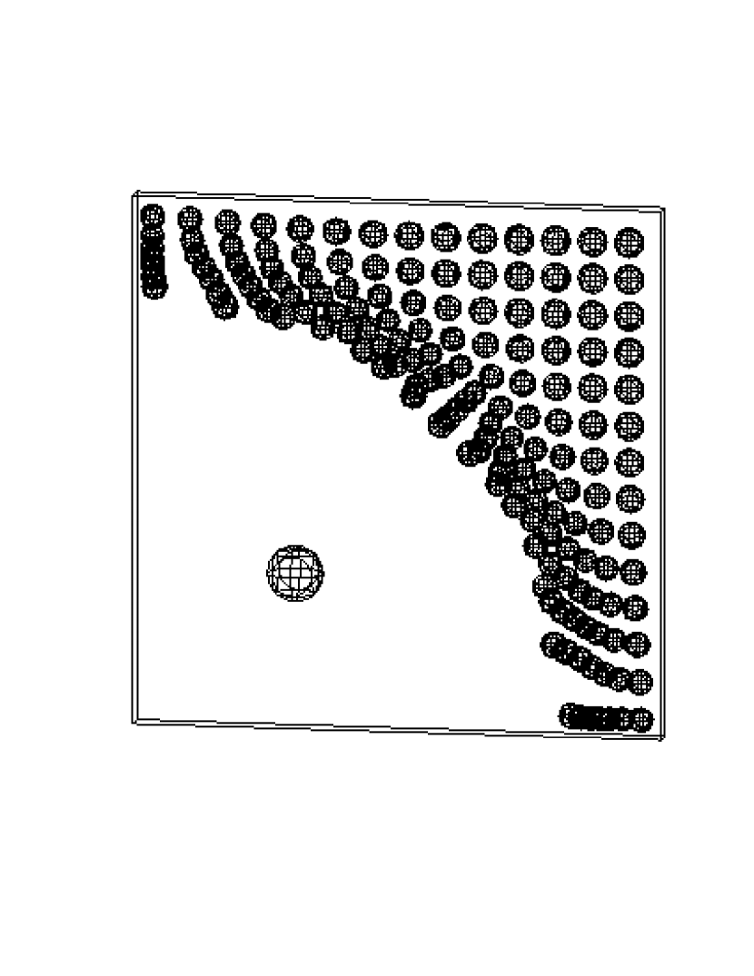
Figure 15 presents kernel plots for the ASPH and SPH 3D Sedov blastwave simulations at time $t=0.1$. We only plot a thin slice through the volume (selecting out a single plane of nodes) for clarity. It is clear that the ASPH kernel shapes are indeed flattening radially as expected, while the SPH nodes show relatively little change in the expanding shockfront. This difference is expected, since in 3D the ASPH ${\bf G}$ tensors are still able to approach the $\rho^{-1}$ evolution of the smoothing scale in the radial direction, while the SPH smoothing scales are constrained to evolve much more slowly as $\rho^{1/3}$. Also, as is evident in 2D, the ASPH nodes in 3D retain their ability to adapt to the physical, spherical geometry of the problem well, avoiding the grid based artifacts evident in the SPH node distribution.

Figure 16: Average radial density profiles for ASPH (open squares) and SPH (crosses) 3D Sedov blastwave simulations at times $t$ = 0.01, 0.04, 0.07, and 0.10. Each point represents an average of a radial bin containing 50 nodes. The solid lines show the Sedov solution.

Figure 17: Average radial profile of density $\rho(r)$, pressure $P(r)$, and radial velocity $v_{r}(r)$ for 3D Sedov blastwave simulations at $t=0.1$. The squares represent the ASPH result, crosses SPH, and the solid lines show the spherical Sedov solutions.

Figure 18: Evolution of the global energies (kinetic, thermal, and total) for the 3D Sedov blastwave simulations.

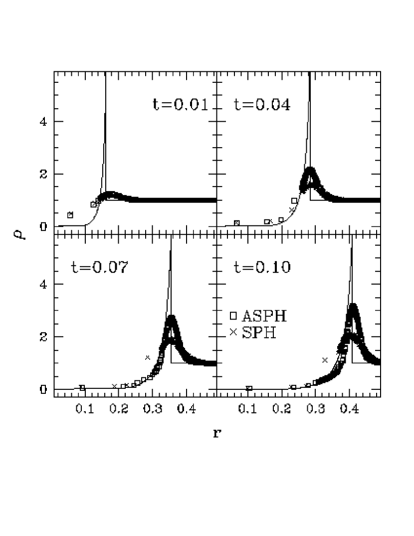
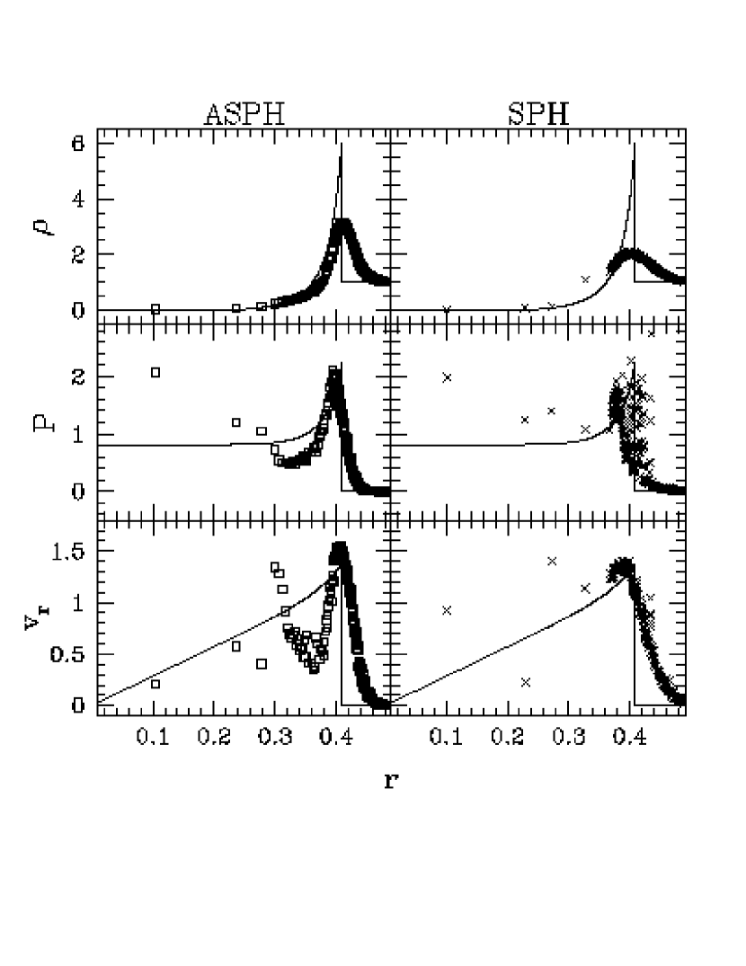
Figure 16 presents a time sequence of radial profiles for these simulations. Each point represents an average of 50 particles in a radial bin. The solid lines show the Sedov similarity solution predictions. The lower resolution of these simulations in comparison with the 2D simulations is quite evident, as both simulations fall well short of the predicted density jump $\rho_{2}/\rho_{1}=6$. If as in the 2D case we examine the typical compression of an ASPH kernel in the shock front, we find that typically the ratio of the shortest to longest axis is $h_{3}/h_{1}\sim 0.4$, as compared with the theoretical prediction $6^{-1}\sim 0.167$. Nevertheless, it is clear that ASPH is still able to resolve the density jump more effectively than SPH, exceeding SPH’s maximum density by $50\%$ at $t=0.1$ and localizing the shock more precisely. Figure 17 plots the radial profiles of the density, pressure, and velocity at $t=0.1$ of both simulations against the analytical solutions. It is evident that that ASPH is better able to reproduce the analytical profiles in all these quantities, though again the lack of resolution due to paucity of particles hurts both simulations. Finally, Figure 18 shows the evolution of the global energies. In this case ASPH conserves energy to better than $\Delta E/E\sim 1\%$, while SPH conserves to $\Delta E/E\sim 0.1\%$.

4.1.3 Riemann Shocktube Test

The Riemann shocktube is a well-known test problem to which SPH codes are traditionally subjected (Monaghan & Gingold 1983; HK89; Rasio & Shapiro 1991). This problem is also examined in Paper I, but only with a 1D code. We reexamine it here since the ASPH formalism differs from that of Paper I, and because the treatment here is 2D. As this is such a well-known problem, we will only briefly outline the setup. The initial conditions consist of placing two regions of gas, differing in density and pressure, adjacent to one another across an interface. This discontinuity will collapse in a quasi-analytically known manner. Because this problem requires a fairly large number of nodes along the collapse dimension to get reasonable results, we have chosen to initialize it in a slightly different manner than previous problems. In this case, our computational volume is a rectangular strip (of aspect ratio 4:1) with the long axis aligned with the direction of collapse. This allows us to have more of our nodes in the direction of interest, while still maintaining a 2D simulation. We should also note that since this simulation is periodic, we in fact have two shocktubes evolving in our volume. Therefore, even though we have 150 rows of particles along our $x$ dimension, we really only have 75 rows per shocktube. All ${\bf G}$ tensors are initialized as circular SPH ${\bf G}$ tensors appropriate for the local density. Table 3 presents the major simulation parameters for this test.

Figure 19: Kernel plots for 2D Riemann shocktube simulations at $t=0.15$. Shown are ASPH (left panel) and SPH (right panel) simulations.

Figure 20: Profiles of mass density $\rho(x)$, pressure $P(x)$, and velocity $v_{x}(x)$ along the $x$ axis for the ASPH (squares) and SPH (crosses) 2D Riemann shocktube simulations at $t=0.15$. Solid lines show the analytical profiles.

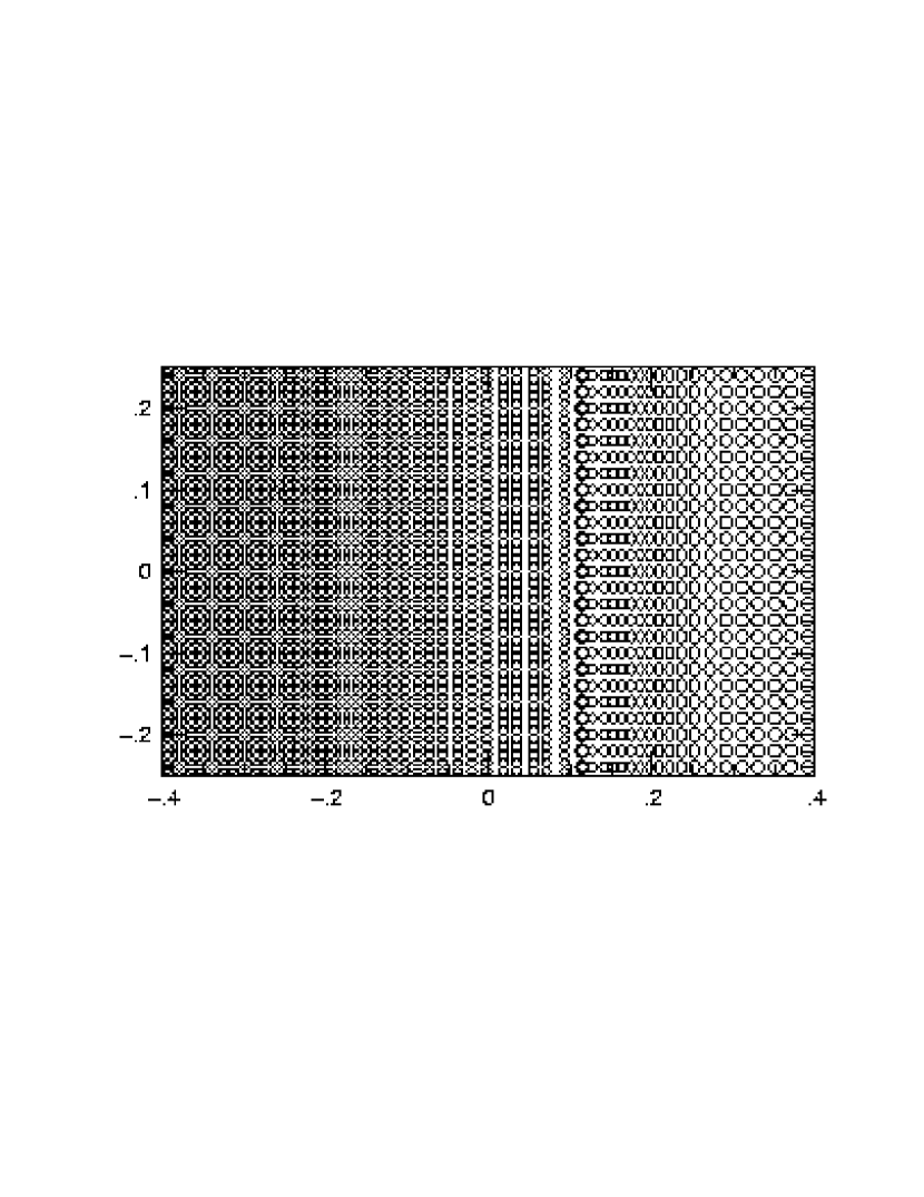
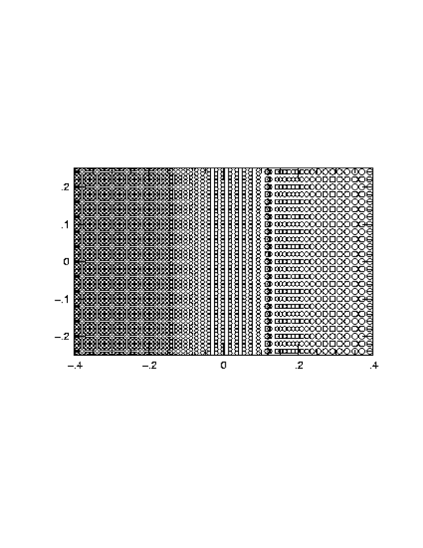
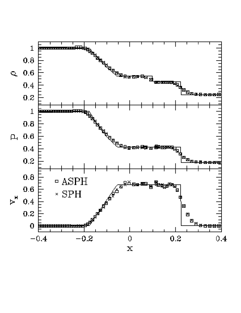
Figure 19 shows kernel plots for a region including one of the shockfronts at $t=0.15$, the end state of the simulations. Note that the ASPH ${\bf G}$ tensors are only slightly deformed by the relatively gentle density evolution of this problem, with axis ratios in the range $h_{2}/h_{1}\in[0.63,1.0]$, $\mbox{$\left\langle h_{2}/h_{1}\right\rangle$}=0.87$. Figure 20 shows the $x$ profiles for the mass density $\rho$, pressure $P$, and velocity $v_{x}$ for the regions shown in Figure 19, along with the analytic solutions for these quantities. We plot all nodes in this region, so each point plotted actually represents many overlapping points as we project in the $y$ direction through the system. There is little evidence for symmetry breaking, as the points overlap nicely. ASPH and SPH appear to solve this problem equivalently, with little distinction between the two. This is not surprising, as the density evolution is fairly gentle and therefore there is little need for large dynamic range in the resolution scale.

4.1.4 Two Interacting Blast Waves

We will now discuss a test problem popularized by Woodward & Colella (1984), which has become a fairly standard hydrodynamic test. This problem involves multiple interactions of strong shocks, rarefaction waves, and contact discontinuities, and is in general a rather stringent test. The initial conditions are discussed in detail in Woodward (1982) and Woodward & Colella (1984), so we only summarize here. A $\gamma=1.4$ gas is initialized at unit density ($\rho=1$) in a unit length. Three regions of differing pressure are established according to

$$P(x)=\left\{\begin{array}[]{l@{\quad}l}1000,&x\in[0,0.1];\\ 0.01,&x\in[0.1,0.9];\\ 100,&x\in[0.9,1].\end{array}\right.$$ (29)

The system is evolved within reflecting boundary conditions. Note that these initial conditions result in two strong blast-waves (of Mach numbers $\sim 170$ and $\sim 51$ respectively) propagating toward one another through the low pressure gas, as well as two rarefaction waves moving backwards through the hot gas. In addition to Woodward & Colella’s comparisons, this problem has also been investigated under 1D SPH by Steinmetz & Müller (1993) and in 2D under the free Lagrangian method by Whitehurst (1995). In order to mimic the reflecting boundary conditions, we use a periodic volume with the initial conditions of equation (29) mirrored about $x=0$. Additionally, as in the previous Riemann shocktube this problem requires a fair degree of linear resolution in the direction of evolution, so we evolve the system in a rectangular strip of gas. Even using an exceedingly thin strip of gas we still only have marginal resolution along the direction of interest (256 nodes in the cases shown here). Table 4 summarizes our major simulation parameters for this test.

Figure 21: Kernel plots for the 2D Woodward double blastwave simulations at $t=0.038$ in the sub-region ($x\in[0.55,0.9],y\in[0,0.125]$). Shown are ASPH (left panel) and SPH (right panel).

Figure 22a: Velocity ($v_{x}$) and mass density ($\rho$) profiles plotted against $x$ for the ASPH simulation of the 2D Woodward double blastwave problem. Shown are profiles for times $t$ = 0.01, 0.016, 0.026, 0.028, 0.030, 0.032, 0.034, and 0.038, which are chosen for direct comparison to the corresponding figures in Woodward & Colella (1984) and Steinmetz & Müller (1993).

Figure 22b: Velocity ($v_{x}$) and mass density ($\rho$) profiles plotted against $x$ for the SPH simulation of the 2D Woodward double blastwave problem. Panels selected and arranged as in Figure 22a.

Figure 25: Evolution of the global energies (kinetic, thermal, and total) for the 2D Woodward double blastwave simulations.

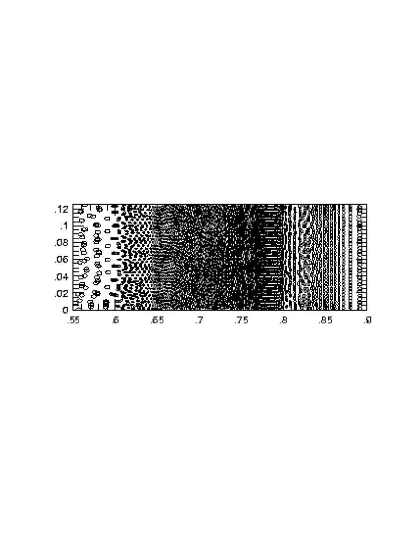
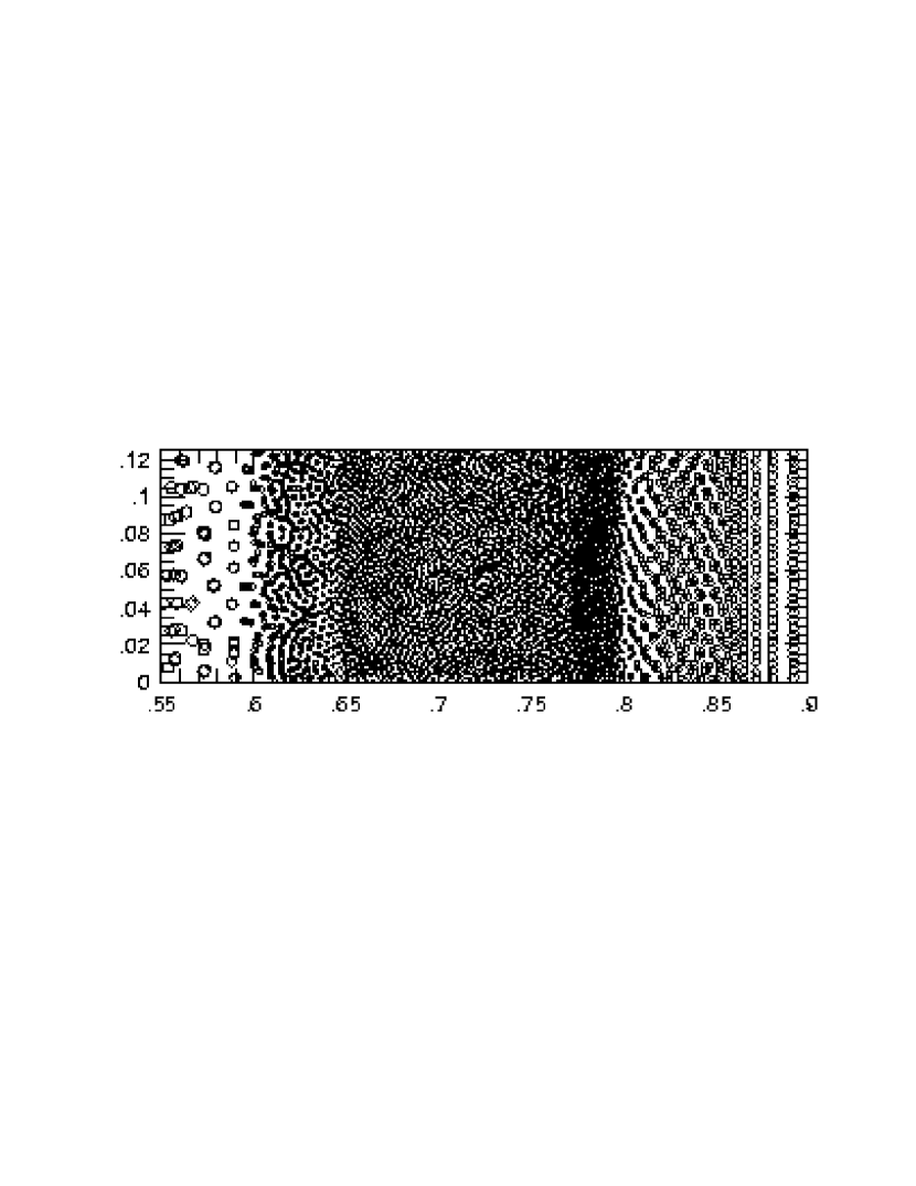
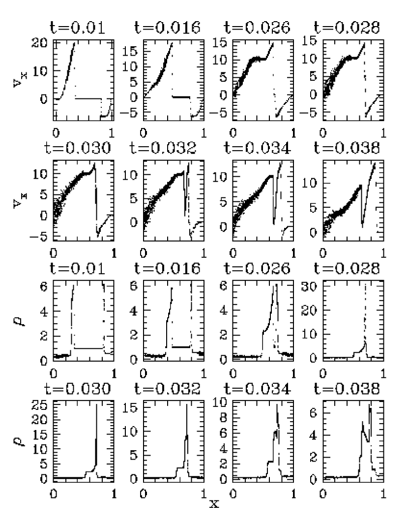
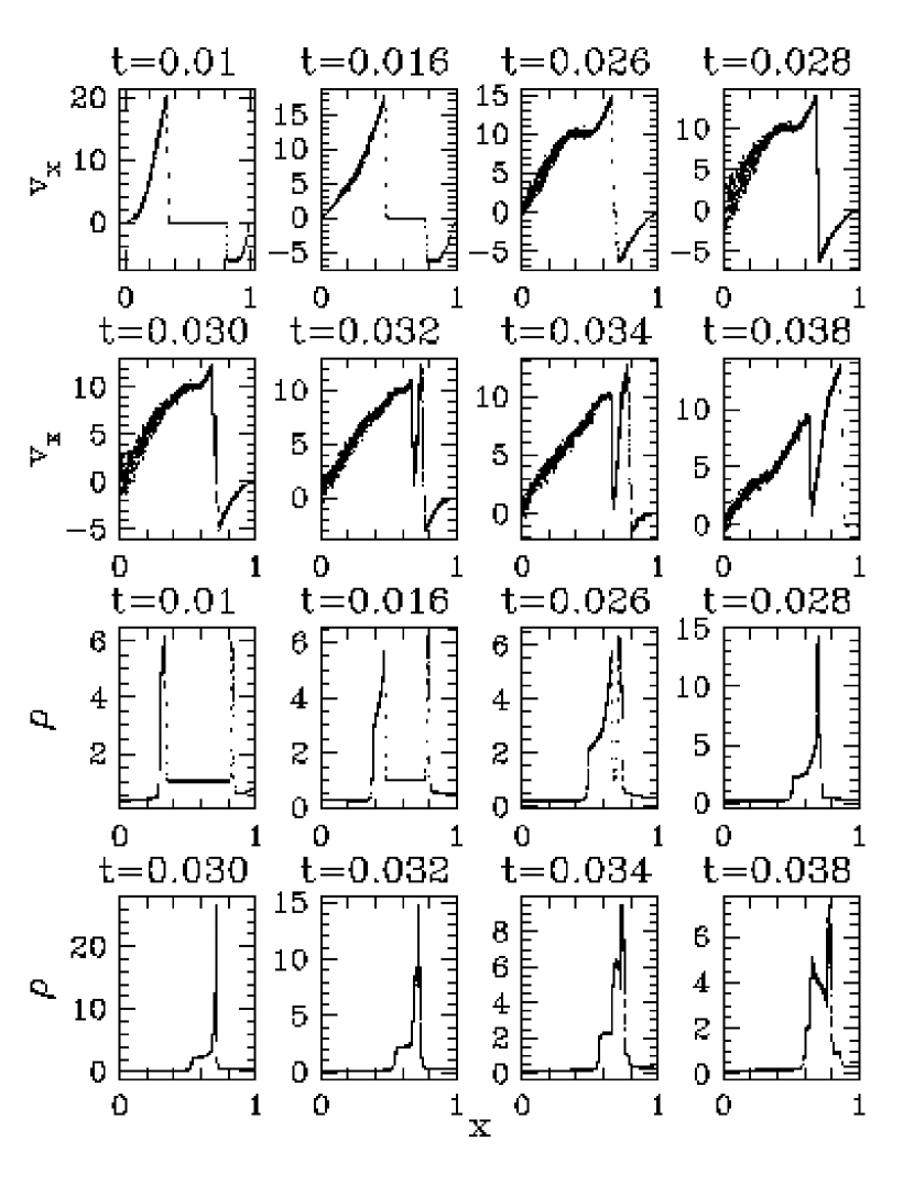
Figure 21 shows kernel plots for the region $(x,y)\in([0.55,0.9],[0,0.125])$ at the end state $t=0.038$ of these simulations. In accordance with the 1D nature of this problem, the ASPH ${\bf G}$ tensors adapt primarily in the $x$ direction, and remain marginally better ordered (closer to the initial lattice) than the SPH case. Figures 22aa & b show the velocity and mass density profiles for these simulations at the same times slices shown in both Woodward & Colella (1984) and Steinmetz & Müller (1993), in order to facilitate comparison. Both ASPH and SPH represent this problem reasonably well, though note that at time $t=0.028$ (just as the two shockfronts collide) the ASPH simulation resolves a much higher density spike (of order $\rho_{peak}\sim 30$), as compared with SPH (which finds $\rho_{peak}\sim 14$). The predicted value for this density jump is 24, so ASPH slightly overshoots. The higher ASPH value is a direct result of ASPH’s ability to achieve superior spatial resolution in this small region. We also note that in the regions where there is evident disorder in these profiles (particularly behind the rarefaction wave moving through the initially $P=1000$ gas) the system is hitting the maximum smoothing scale we can allow due to the narrow width of the simulation, so some fraction of this scatter is in fact likely an artifact. In general, as found by Müller & Steinmetz (1993), both SPH and ASPH seem capable of solving this problem, despite the commonly held belief that SPH cannot deal with strong shock phenomena.

4.2 2D Test Cases

Figure 26: Gray-scale images of the SPH estimated components $\left\langle\partial v_{\alpha}/\partial x_{\beta}\right\rangle$ for a bar in solid-body rotation with angular velocity $\omega$. These quantities formally should be constant throughout the bar.

Each of the previous test cases represent idealized situations with no “handedness” to the problem (i.e. they are physically 1D). Additionally, due to the physical symmetry of these 1D problems, the ${\bf G}$ tensors are able to align themselves such that all significant interactions take place along one of their major axes. In this section we will investigate problems which break these symmetries and are truly 2D, concentrating on rotational test cases in order to investigate the question of angular momentum conservation under ASPH (discussed in §3.4). Specifically we will examine a gas disk subjected to an external Keplerian potential (§4.2.1) and a self-gravitating disk undergoing radial collapse with rotation (§4.2.2).

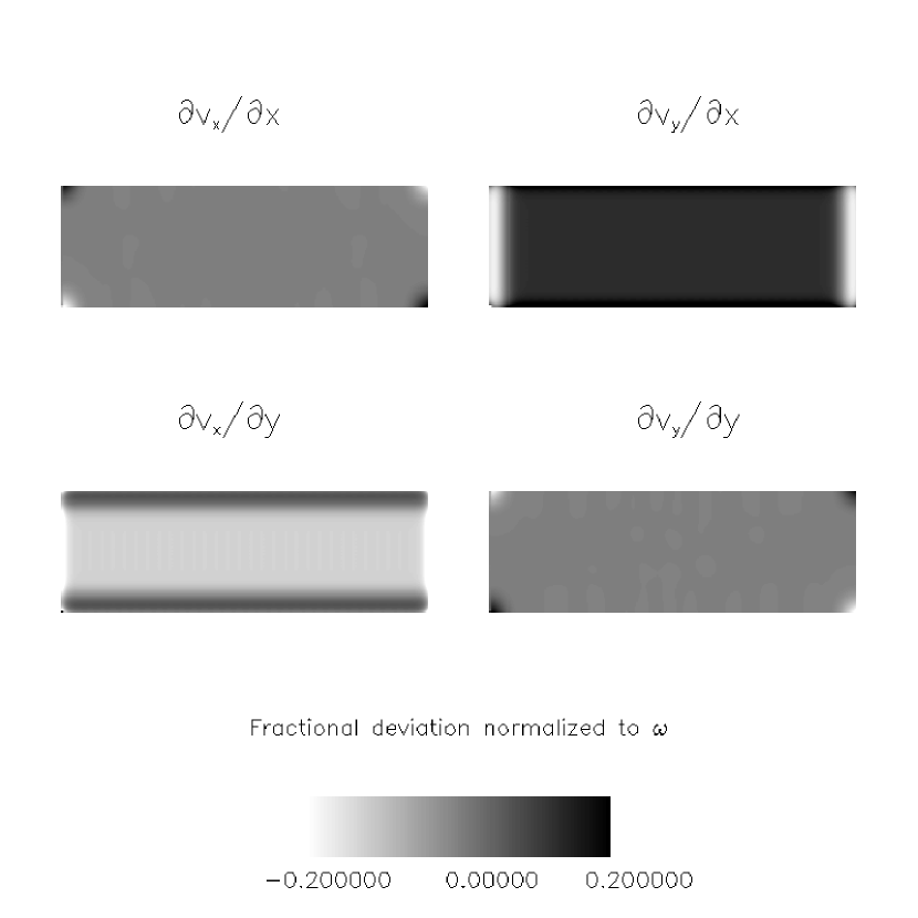
Before we begin this discussion, though, we should address why we do not examine an obvious test case for angular momentum. The simplest example of a problem with a well-defined angular momentum is a rigidly rotating bar, something with an equation of state like a solid so that it should simply maintain solid body rotation. There is, however, an unfortunate flaw with such a deceptively simple system, which is that it possesses an edge. (A)SPH is derived assuming that there are no distinct surfaces or edges present in a modeled system, but rather that all quantities vary smoothly. (A)SPH sampled averages, such as defined by equations (1)-(2), will be in error near an edge. Of particular concern for ASPH is the fact that the estimates for the spatial gradients of the velocity field $\left\langle\partial v_{\alpha}/\partial x_{\beta}\right\rangle$ (eq. [15]) will be in error near any edges, which ensures that the evolution of the ${\bf G}$ tensor will also be incorrect. Figure 26 presents images of the SPH estimates of the elements of $\left\langle\partial v_{\alpha}/\partial x_{\beta}\right\rangle$ for a 2D bar rigorously in solid body rotation. If these estimates were correct, then the images should be uniform throughout. This figure clearly shows that, as expected, the SPH estimates are in error near the edges, by as much as $50\%$. So long as this is the case, the ${\bf G}$ tensors near the edges of the system will not be evolved correctly, resulting in a false torque about the surface, and thereby violating angular momentum conservation. We have in fact found this to be the case for ASPH simulations of such systems, and the magnitude of the angular momentum violation scales as the number of surface nodes in the system. It is interesting to note that SPH cannot deal with surfaces any better than ASPH (see, e.g., Monaghan 1992), but because by construction SPH cannot violate global angular momentum conservation, such tests are meaningless. This is simply an example that global conservation alone does not guarantee a successful simulation. Fisher & Owen (1997) are currently investigating a modified technique based upon SPH designed to account and correct for such problems.

In order to investigate the angular momentum issue, it is necessary to study a non-periodic system, which requires the density fall to zero at some point. For this reason, we have investigated rotating disk systems in this paper, in an effort to have the density fall off smoothly to an edge. The fact that there is still an edge is somewhat worrisome, but by having the density fall off smoothly we hope to moderate this problem. Additionally, these sort of systems are more representative of the sorts of rotating problems we are likely to encounter in cosmological structure formation scenarios, such as if we were to model a disk galaxy.

4.2.1 Pseudo-Keplerian Disks

Our first rotational test is a type of Keplerian disk, modified to include pressure support. Since this is not a standard test case, we will describe the initial conditions in some detail. A gas disk is created in rotational and pressure balance with a fixed, external gravitational potential produced by a theoretical point mass at the disk’s center. The initial radial density and pressure profiles of the disk are chosen arbitrarily. The disk is not self-gravitating. In order to make this problem computationally feasible, it is necessary to use a softened potential for the point mass

$$\Phi(r)=-\frac{GM}{(r^{2}+r_{c}^{2})^{1/2}}\quad\Rightarrow\quad{\bf g}(r)=-\frac{GM{\bf r}}{(r^{2}+r_{c}^{2})^{3/2}},$$ (30)

where $M$ is the mass of the gravitating point mass and $r_{c}$ is the softening core radius. Note that the nodes in this gravitational potential are treated as point masses in 3D, not as infinite rods (as was the case for the Zel’dovich pancake simulations). We are now simulating gas confined to a plane.

The forms we choose for the initial radial mass density and pressure profiles are

$$\rho(r)=\rho_{0}\left(1-\frac{r^{2}}{r_{d}^{2}}\right),$$ (31)

$$P(r)=K\rho^{2}(r)=K\rho_{0}^{2}\left(1-\frac{r^{2}}{r_{d}^{2}}\right)^{2},$$ (32)

where $\rho_{0}$ is the central gas density, $r_{d}$ is the outer radius of the gas disk, and $K$ is a constant which sets the amount of pressure support. Based on these choices, the balancing rotational velocity of the gas is

$$v_{t}^{2}(r)=\frac{GMr^{2}}{(r^{2}+r_{c}^{2})^{3/2}}-4K\rho_{0}\frac{r^{2}}{r_{d}^{2}},$$ (33)

where $v_{t}(r)$ is the supporting circular (or tangential) velocity. Equation (33) limits the possible range of the pressure constant $K$ to

$$K\in\left[0,\;\frac{GMr_{d}^{2}}{4\rho_{0}(r_{c}^{2}+r_{d}^{2})^{3/2}}\right].$$ (34)

We generically choose the largest possible value for $K$ in order to maximize the amount of pressure support. Note that maximizing $K$ in this fashion sets $v_{t}(r_{d})=0$.

There is no physical motivation for choosing this problem to study. Rather, this test is designed solely for the purpose of testing ASPH. Since there is no preferred resolution direction, ASPH has no real advantage under this problem. Therefore ASPH’s extra degrees of freedom, rather than offering a real advantage, can only lead to trouble. For $r>r_{c}$, this system possesses a strong radial velocity shear, which will tend to elongate the ASPH ${\bf G}$ tensors into the flow. This is a shear field that cannot be represented under the first-order treatment our ${\bf G}$ evolution derivation is based upon. The problem can be understood by considering the evolution of a hypothetical fluid element in such a Keplerian potential: for $r>r_{c}$ a true fluid element will distend and eventually be infinitely sheared around an arc of the disk. This creates a situation which our first-order derivation of ${\bf G}$ and its evolution cannot ideally adapt to (an ellipse cannot be distorted to follow such a curving arc and remain an ellipse). Therefore our evolution equations for the ${\bf G}$ tensor field must fail at some level for this case. Additionally, the imposed point mass potential is very strongly centralized, whereas our initial density profile is flat-topped. This situation is unstable, and although the system is born in radial balance, we can expect as it evolves it will rapidly deviate from the initial conditions. These effects will tend to force the ASPH ${\bf G}$ tensor field to evolve under conditions it cannot simply, nor ideally, adapt to. Finally, our use of an external central force as the binding global potential will rigorously ensure angular momentum conservation for the gravitational interactions. Any angular momentum errors incurred are therefore due to either numerical problems or ASPH.

In order to initialize the (A)SPH node positions, we first select candidate positions quasi-randomly based on the Sobol sequence. These potential positions are subjected to a Monte-Carlo acceptance/rejection scheme, with a probability distribution appropriate to match the density profile of equation (31). Once a node position is selected, the specific thermal energy is uniquely identified by the required pressure profile in combination with the theoretical density. The ${\bf G}$ tensors are initialized as SPH ${\bf G}$ tensors with determinants $|\mbox{${\bf G}$}|$ scaled appropriately for the theoretical local density. The system is evolved until it is seen to settle into an apparently equilibrium distribution. Finally, in order to obtain meaningful measurements of the angular momentum, these simulations are evolved in a non-periodic computational volume. Table 5 summarizes our input numerical parameters for these simulations.

Figure 27: Kernel plots for the 2D Pseudo-Keplerian Disk simulations at $t=3.0$ for the cases of ASPH (left panel) and SPH (right panel). Arrows are drawn for each node indicating the direction and magnitude of their velocity.

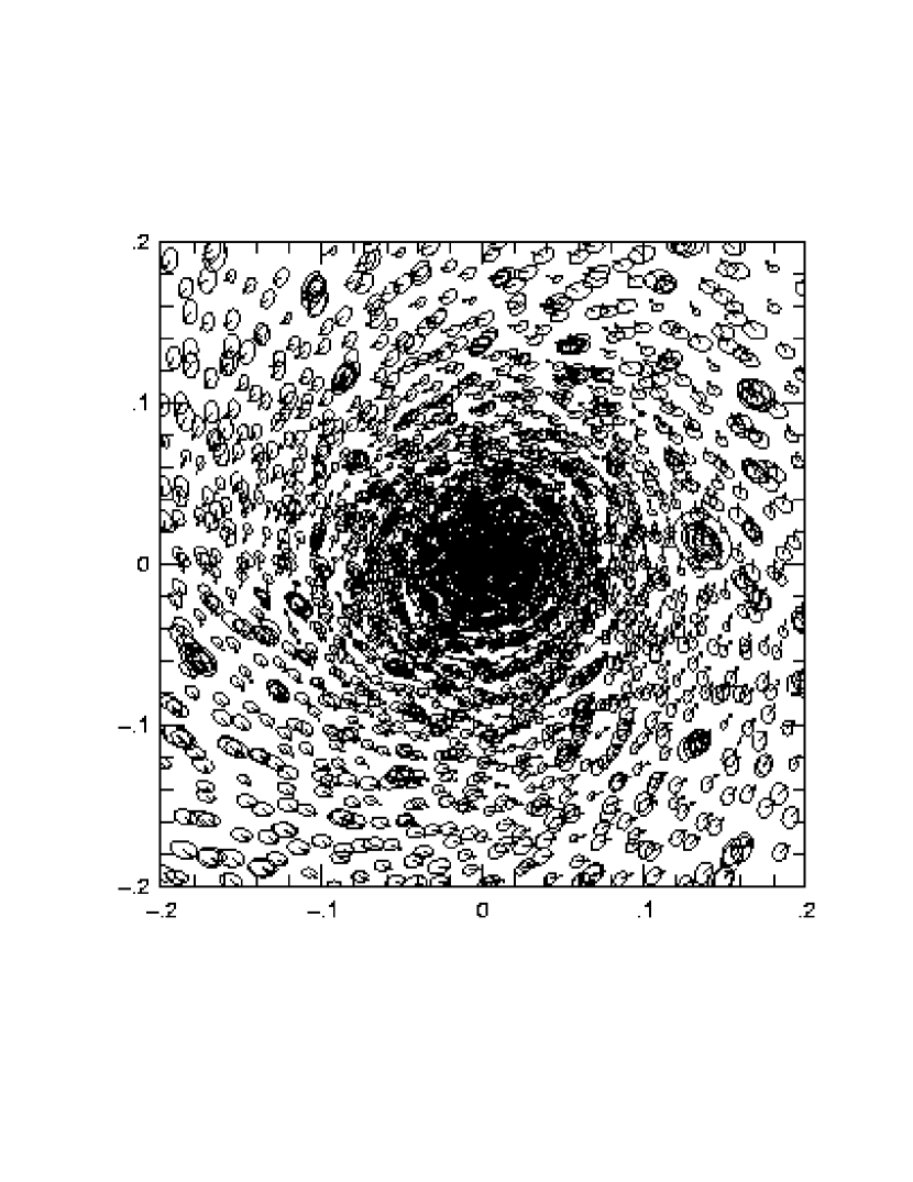
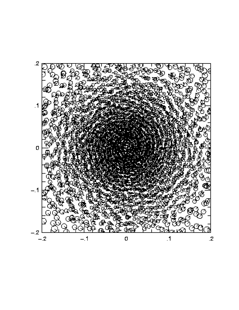
Figure 27 shows kernel plots of the central core regions for both the ASPH and SPH simulations at $t=3.0$. In order to emphasize the steady rotation field, we also plot arrows for each node indicating both the direction and relative magnitude of the velocity. Though grossly similar, there are interesting differences in these two simulations. It appears that the core of the ASPH simulation is relatively denser or more collapsed as compared with SPH. The ASPH kernels seem to be elongated into the direction of rotation, and there is an apparent trend for the ASPH kernels’ ellipticity to increase with radius. The geometry of the ${\bf G}$ tensors ranges from $h_{2}/h_{1}\in[0.5,1.0]$, $\mbox{$\left\langle h_{2}/h_{1}\right\rangle$}=0.75$. This behaviour is understandable in terms of our smoothing algorithm. At all radii the rotational shearing field tends to elongate the ${\bf G}$ tensors into the direction of rotation. At “small” radii ($r/h\sim 1$), the requirement that each node sample several neighbors implies that each sees neighboring nodes which are significantly further around the arc of rotation, and therefore will be trying to elongate their ${\bf G}$ tensors in noticeably different directions. When the ${\bf G}$ tensor field is smoothed, averaging over many different $\mbox{${\bf G}$}_{i}$’s elongated in different directions will result in an average round shape. As we move out to larger radii ($r/h\gg 1$), this averaging process will progressively sample more and more “local” conditions. In this case, each ASPH node sees itself embedded within a coherently shearing field, with neighbors elongating in a similar manner. Averaging in this case retains the elliptical shape, though limits how elliptical each element can become. This sort of behaviour is desirable. When an ASPH node is in a region where on scales of $h$ there are conflicting signals dictating the evolution of ${\bf G}$, the “safest” choice is for ${\bf G}$ to adopt a round shape, emulating SPH. This reflects the fact that the evolution of the ${\bf G}$ tensor is based upon approximating the local velocity field by the first-order argument ${\bf v}({\bf r}+d{\bf r})\approx{\bf v}({\bf r})+\mbox{\boldmath$\sigma$}~{}d{\bf r}$. If this approximation is invalid, then the evolution equations for ${\bf G}$ break down. Only when there is a clear, unambiguous signal dictating the evolution of ${\bf G}$ should it be allowed to deviate from this “safe” choice.

Figure 28: Azimuthally averaged radial mass profiles for the 2D Pseudo-Keplerian Disk simulations. Each curve represent the fraction of the mass of the disk contained within the radius $r$ at a particular time. The top panels show the function $M(r)$ for times varying from the beginning of the simulation to the end ($t\in[0,3]$). The bottom panels show only the last 6 measurements of $M(r)$, in the time range $t\in[2.5,3]$.

Figure 29: Azimuthally averaged radial density profiles for the 2D Pseudo-Keplerian Disk simulations, expressed as a function of the enclosed mass fraction $\rho(\mbox{$M_{\mbox{\scriptsize interior}}$})$. The top panels show the function $\rho(\mbox{$M_{\mbox{\scriptsize interior}}$})$ for times varying from $t\in[0,3]$, while the bottom panels only show the last few measurements at times $t\in[2.5,3]$.

In order to examine these different mass distributions in a more quantitative fashion, Figures 28 and 29 show the distribution of $M(r)$ and $\rho(M)$ respectively, measured radially outward from the center of the potential. Note that these two figures are plotted subtly differently: Figure 28 shows the mass fraction as a function of radius $M(r)$/$M_{\mbox{\scriptsize tot}}$, whereas Figure 29 shows the density distribution as a function of the radially enclosed mass fraction $\rho(\mbox{$M_{\mbox{\scriptsize interior}}$}/\mbox{$M_{\mbox{\scriptsize tot}}$})$. Each figure plots many curves: the upper panels show the evolution of these functions from the beginning to the end of the simulations, while the lower panels only show the final few measurements. It is evident that in the beginning the mass distribution evolves fairly steadily up to a point, and then settles into an equilibrium (or at least slowly evolving) state. In Figure 28 we can see that the total ASPH mass distribution is slightly more diffuse than SPH, indicating more mass has been thrown to the outer regions of the disk or become unbound. Figure 29 also shows that the core of the ASPH disk is more dense than the SPH by a little more than a factor of two, confirming the visual impression of the kernel plots.

Figure 30: Azimuthally averaged radial measurements of angular momentum $\Delta L_{z}$ as a function of the enclosed mass for the 2D Pseudo-Keplerian Disk simulations. These curves represent a radial measurement of $dL_{z}/dM$, where $M$ is interpreted as the radially enclosed mass. The top panels show the function $dL_{z}/dM$ for times varying from $t\in[0,3]$, while the bottom panels only show the last few measurements at times $t\in[2.5,3]$.

Figure 31: The total enclosed angular momentum $L_{z}$ as a function of the enclosed mass $M$ for the 2D Pseudo-Keplerian Disk simulations, as measured radially from the center of the disk. These curves of $L_{z}(M)$ represent the integration $\int_{0}^{M}(dL_{z}/dM)dM$ of the function $dL_{z}/dM(M)$ presented in Figure 30.

Figure 32: Evolution of the global energies (left panel: kinetic, thermal, potential, and total) and the total angular momentum $L_{z}$ (right panel) for the 2D Pseudo-Keplerian Disk simulations.

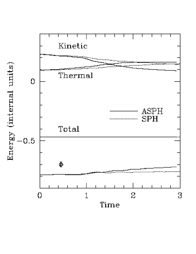
Our primary interest in this problem is the evolution of the angular momentum. Figure 30 shows the function $dL_{z}/dM(M)$, which is the amount of angular momentum contained in shells as a function of the total mass interior to that shell. Figure 31 shows the integration of this function $L_{z}(M)=\int_{0}^{M}(dL_{z}/dM)dM$, which represents the total angular momentum contained within the mass fraction $M$. Since this problem should settle to a condition of axisymmetry, we expect that the radial angular momentum distribution should settle to a steady state. It is evident from Figure 30 that the radial distribution of $dL_{z}/dM$ initially changes rather rapidly, and then settles for both simulations to a fairly steady configuration. The ASPH and SPH distributions of angular momentum are somewhat different, however. ASPH settles into a nearly linear distribution of $dL_{z}/dM$ with respect to increasing mass, while SPH characteristically maintains more angular momentum in the core region. These differences are expected since ASPH finds a denser core, and therefore must lose more angular momentum from the core mass. Nevertheless, both simulations do converge to equilibrium, rotating configurations. Figure 32 shows the evolution of the global energies and angular momentum. SPH of course conserves global angular momentum nearly exactly (by construction), while ASPH suffers an overall fluctuation $\Delta L_{z}/L_{z}\sim 3\%$.

Since we do not have an analytical expectation for this problem, it is difficult to know which technique better represents the “true” solution. However, we can state that ASPH appears to conserve the global angular momentum reasonably, and also does not seem to suffer dramatic local transport problems (as evidenced by the fact that the local radial angular momentum distribution establishes an equilibrium state). It is worth noting that smoothing the ${\bf G}$ tensors is critical for this problem. In all of the previous tests we found that smoothing ${\bf G}$ has relatively little impact on the outcome. However, in this case, without smoothing the ${\bf G}$ tensors rapidly become extremely distorted in the shearing velocity field, which leads to poor angular momentum conservation (angular momentum losses $\Delta L_{z}/L_{z}\sim 100\%$ in a single rotation or two). These extreme distortions in the individual ${\bf G}$ tensors are unphysical, since they are trying to track neighboring ASPH nodes around the arc of rotation, which they cannot do. Smoothing the ${\bf G}$ tensors limits this process and keeps the distortion manageable, though there may ultimately prove to be a better solution.

4.2.2 Collapsing Disk with Rotation

The Pseudo-Keplerian disk simulation offers encouraging evidence that ASPH can solve rotational problems while maintaining reasonable conservation of the angular momentum. However, it is not convincing in and of itself. Although the Pseudo-Keplerian disk does undergo significant radial evolution, this evolution is relatively gentle in time, and does not involve strongly distorting the ${\bf G}$ tensors themselves. This is mainly due to the fact that the only strong signal to drive the evolution of the ${\bf G}$ tensors is the shearing rotational field. We now wish to propose a more stringent test of angular momentum conservation, in which we can expect significant evolution of the ${\bf G}$ tensors right down into the core, at least initially. In order to accomplish this, we simulate a modified form of a standard Maclaurin disk (Binney & Tremaine 1987), which is an analytically tractable class of rotating hydrodynamic disks. The modification we make to this problem is to take away the majority of its pressure support, making the system unstable to collapse. When the timescale for collapse is significantly shorter than the rotational timescale, the collapse process will dominate the ${\bf G}$ tensor evolution. Additionally, a rotational problem undergoing rapid and violent collapse presents a difficult problem both in terms of the transport and conservation of angular momentum, making this an overall much more difficult test.

As the Maclaurin disk is a well-documented problem, we will only briefly outline this setup here, emphasizing our modification of the pressure term. The Maclaurin disks represent a class of gas disks which have radial density, pressure, and circular velocity profiles

$$\rho(r)=\rho_{0}\left(1-\frac{r^{2}}{r_{d}^{2}}\right)^{1/2},$$ (35)

$$P(r)=fK\rho^{3}(r),$$ (36)

$$v_{t}(r)=\Omega r,$$ (37)

$$\Omega\in[0,\Omega_{0}],\quad\quad\Omega_{0}^{2}=\frac{\pi^{2}G\rho_{0}}{2r_{d}},$$ (38)

where $\rho_{0}$ is the central density, $r_{d}$ the disk radius, $K$ a constant normalizing the pressure, $f\in[0,1]$ a multiplicative fudge factor, $\Omega$ the frequency of rotation, and $\Omega_{0}$ the natural frequency of the system. Our modification is the introduction of $f$, which allows us to tweak the fraction of the required pressure support actually introduced into the system. If we set $f=1$ we recover the traditional Maclaurin disk problem, for which solid body rotation provides radial balance. For $f<1$, the pressure support is inadequate and the disk becomes unstable to collapse.

As with the Pseudo-Keplerian disk, this simulation is performed in a non-periodic computational volume in order make measurements of the global angular momentum meaningful. We solve for the self-gravity utilizing a non-periodic PM code. The gravity calculation treats the nodes as points in 3D, so we are again considering gas confined to a plane in a 3D space rather than infinite parallel rods. In order to seed the initial positions of the (A)SPH nodes to match the density profile of equation (35), we select candidate positions using a Sobol sequence which are subjected to a monte-carlo acceptance/rejection criterion. All ${\bf G}$ tensors are initialized as round SPH ${\bf G}$ tensors, scaled appropriately for the local theoretical density. Table 6 summarizes our major numerical parameters for these simulations.

Figure 33: Kernel plots for the 2D collapsing disk simulations. Panels are arranged with time increasing down columns: $t=0.08$ (pre-collapse) in the upper row, $t=0.1$ (maximum collapse) in the middle row, and $t=0.5$ (post-collapse) in the lower row. The ASPH simulation is on the left, and SPH on the right. The arrows associated with each node indicate the direction and magnitude of the velocity.

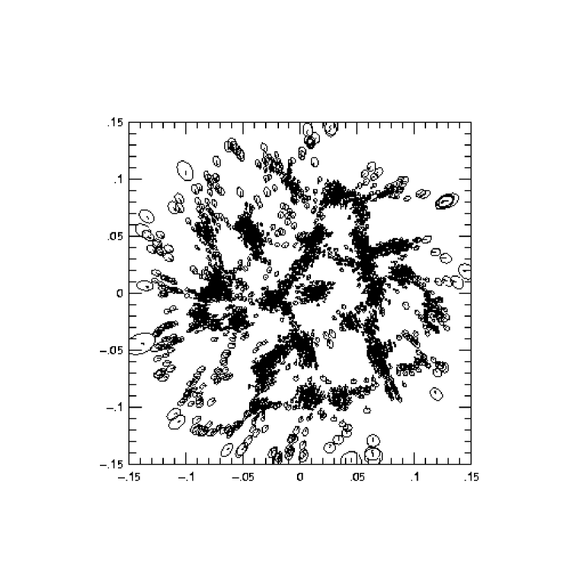
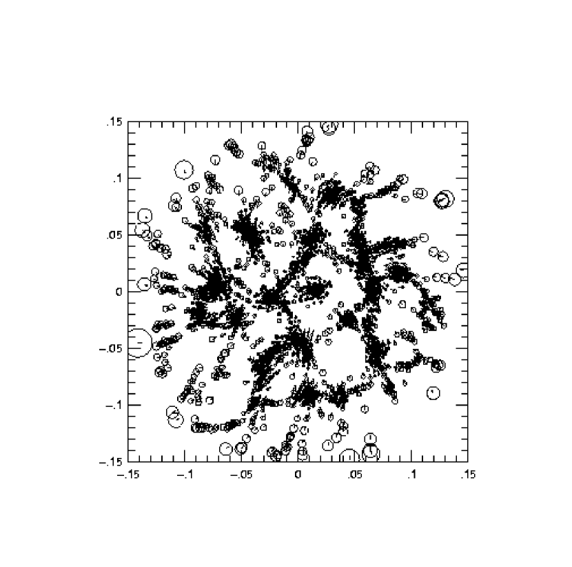
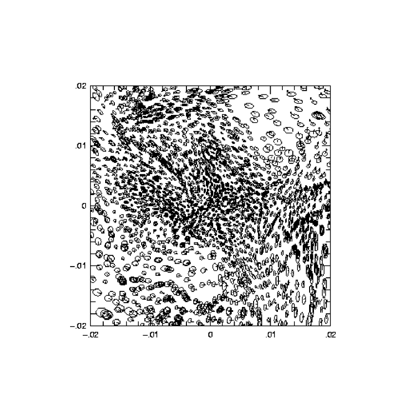
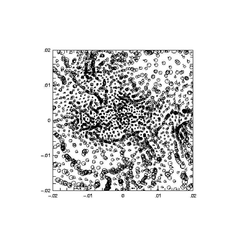
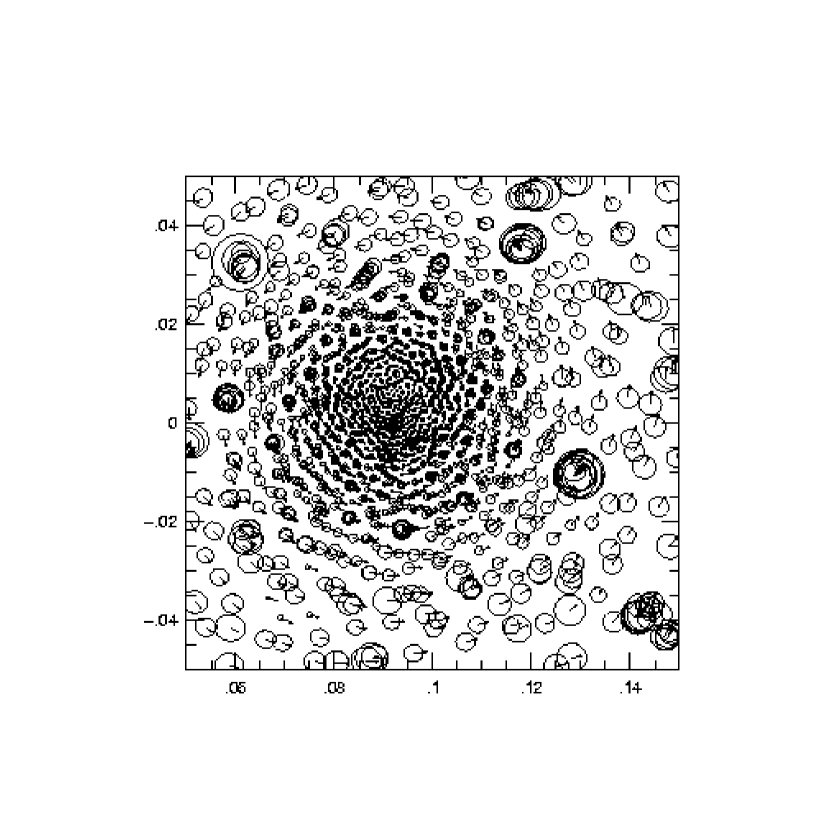
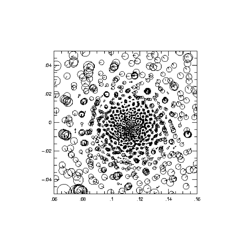
The evolution of this system is quite complex. With $f=0.001$, the system is highly unstable, undergoing immediate, radical collapse. As the overall radial collapse proceeds, the disk fragments into a collection of filaments due to the gravitational amplification of perturbations in the noisy initial density field. During this filamentary stage, the ASPH ${\bf G}$ tensors become quite elliptical, aligning themselves along the filaments. By $t=0.1$ the system reaches maximum collapse, and this filamentary structure is destroyed. After this time, we find that the system settles into a two-phase structure. There is a hot, dense, rapidly rotating core surrounded by a diffuse, slowly expanding halo. Figure 33 presents kernel plots for the ASPH and SPH simulations at times $t=0.08,0.1,0.5$, corresponding to the pre-collapse, maximal-collapse, and post-collapse regimes. We also plot the velocity fields on these kernel plots as vector fields. At $t=0.08$ (top panels), the pre-collapse filamentary structure is evident. During this stage, the ASPH simulation exhibits ${\bf G}$ tensors with ellipticities in the range $h_{2}/h_{1}\in[0.28,0.99]$, $\mbox{$\left\langle h_{2}/h_{1}\right\rangle$}=0.64$. Examining the middle row of panels at $t=0.1$ (the initial point of maximum collapse), there is an evident clumpiness in the distribution of nodes with a large range of smoothing scales. The velocity field demonstrates a rather complex structure, though an overall counterclockwise sense of rotation is maintained, reflecting our input angular momentum. Note that the ASPH simulation shows markedly elliptical kernels in this collapsing core region, with axis ratios in the range $h_{2}/h_{1}\in[0.21,0.98]$, $\mbox{$\left\langle h_{2}/h_{1}\right\rangle$}=0.59$. Despite this, the particle positions and overall fluid flow corresponds well between the ASPH and SPH runs at this time. Finally, at $t=0.5$ in the bottom row of panels, we find that the system settles into orderly rotation about a dense core. The ASPH simulation exhibits basically round ${\bf G}$ tensors in the core (with overall ${\bf G}$ geometries in the range $h_{2}/h_{1}\in[0.46,1.0]$, $\mbox{$\left\langle h_{2}/h_{1}\right\rangle$}=0.92$) reminiscent of the Pseudo-Keplerian Disk, which is appropriate as there is no preferred resolution direction.

Figure 34: Azimuthally averaged radial mass profiles for the 2D collapsing disk simulations. Each curve represent the fraction of the mass of the disk contained within the radius $r$. The top panels show the function $M(r)$ for times varying from the beginning of the simulation to the end ($t\in[0,0.5]$). The bottom panels show only the last measurements of $M(r)$, in the time range $t\in[0.35,0.5]$.

Figure 35: Azimuthally averaged radial density profiles for the 2D collapsing disk simulations, expressed as a function of the enclosed mass fraction $\rho(\mbox{$M_{\mbox{\scriptsize interior}}$})$. The top panels show the function $\rho(M_{interior})$ for times varying from $t\in[0,0.5]$, while the bottom panels only show the last few measurements at times $t\in[0.35,0.5]$.

Figures 34 and 35 show the evolution of the functions $M(r)$ and $\rho(M)$, analogously to Figures 28 and 29 for the Pseudo-Keplerian disk simulations. In this case, though, we measure the radial coordinate out from the center of mass of the central disk, since this is a self-gravitating system and therefore the minimum of the potential moves with the center of mass. It is clear that the system rapidly forms a concentrated central disk containing $\sim 70\%$ of the mass following the maximum collapse. The radial density gradient of this central disk is also quite large, varying from $\rho\sim 10^{3}$ in the central regions to $\rho\sim 10^{-1}$ at the edge. The ASPH and SPH simulations both seem to agree well on this mass distribution.

Figure 36: Azimuthally averaged radial measurements of angular momentum $\Delta L_{z}$ as a function of the enclosed mass for the 2D collapsing disk simulations. These curves represent a radial measurement of $dL_{z}/dM$, where $M$ is interpreted as the radially enclosed mass. The top panels show the function $dL_{z}/dM$ for times varying from $t\in[0,0.5]$, while the bottom panels only show the last few measurements at times $t\in[0.35,0.5]$.

Figure 37: The total enclosed angular momentum $L_{z}$ as a function of the enclosed mass $M$ for the 2D collapsing disk simulations, as measured radially from the center of the disk. The curves of $L_{z}(M)$ represent the integration $\int_{0}^{M}(dL_{z}/dM)dM$ of the function $dL_{z}/dM(M)$ presented in Figure 36.

Figure 36 shows the radial distributions of $dL_{z}/dM(M)$ throughout the simulations. It is evident that once the systems achieve equilibrium, the central $70\%$ of the mass (representing the collapsed disk) maintains a steady distribution of angular momentum. However, outside the collapsed disk this distribution becomes quite noisy for the hot, diffuse gas. It is also curious to note that it appears the ASPH simulation maintains slightly more angular momentum in the disk as compared with SPH. This is also evident in the cumulative distribution of $L_{z}(M)=\int_{0}^{M}(dL_{z}/dM)dM$ in Figure 37. This trend is the opposite that found in the previous Pseudo-Keplerian disk, where SPH maintains a larger core angular momentum than ASPH. Regardless, it is clear that both ASPH and SPH settle to equilibrium distributions of the local angular momentum once the system settles and axisymmetry is achieved.

Figure 38: Evolution of the global energies (left panel: kinetic, thermal, potential, and total) and the total angular momentum $L_{z}$ (right panel) for the 2D collapsing disk simulations.

Finally, in Figure 38 we present the time evolution of the global energies and angular momentum. It is apparent that at time $t=0.1$ the system undergoes maximal collapse, at which time all the energies suffer a dramatic spike. After this time the energies achieve equilibrium values. The global angular momentum for the ASPH simulation varies by $\Delta L_{z}/L_{z}\sim 3\%$ throughout the simulation, while SPH varies by $\Delta L_{z}/L_{z}\sim 1\%$. This error is likely due to the PM code, which does not conserve angular momentum precisely. We therefore conclude that in this test ASPH again conserves angular momentum reasonably, both locally and globally.

5 Summary and Conclusions

A new version of SPH, which we call Adaptive SPH, or ASPH, which replaces the isotropic smoothing of standard SPH by anisotropic smoothing, is described in detail here, along with the results of test problems and comparisons with standard SPH. This is Paper II of a pair of methodology papers describing ASPH and its application to cosmological gas dynamics. In Paper I, we demonstrated the relative shortcomings of SPH compared to ASPH whenever the flow problem to be simulated involves highly anisotropic volume changes, such as occur commonly in cosmic structure formation, involving gravitational collapse and strong shocks. Paper I described the ASPH algorithm in detail, including a mathematical prescription for evolving the ellipsoidal smoothing kernels based upon the idea that each ellipsoid rotates and deforms with the flow so as to track the Lagrangian evolution of infinitesimal fluid elements centered on each SPH particle. In Paper I, this ASPH algorithm was implemented in 2D and tested against a variety of problems like the Riemann shock and cosmological pancake problems, in comparison with standard SPH. In addition to anisotropic smoothing, the ASPH method described in Paper I included an algorithm designed to reduce the spurious effects of artificial viscous heating of gas undergoing supersonic compression far from a shock, by selective inclusion of artificial viscosity in the energy equation only for particles which are close to being overtaken by shocks. The combined effects of anisotropic smoothing and this suppression of viscous heating away from shocks was shown in Paper I to result in a substantial increase in spatial resolving power at fixed particle number, for problems like cosmological pancake collapse, generic to cosmic structure formation.

In Paper II, we have described further developments of the ASPH method, further tests, and an alternative mathematical prescription for the evolution of the anisotropic smoothing kernels. The latter is based upon a linear transformation of spatial coordinates for each particle to one in which the mean spacing of particles in the vicinity of that particle appears to be isotropic. Paper II has described the implementation of this ASPH algorithm in both 2D and 3D. Several refinements of the ASPH scheme described in Paper I are described here, such as the use of separate time-steps for separate particles and a new scheme for nearest-neighbor assignment, which improve the efficiency of the method, and the use of ellipsoidal smoothing kernels whose axis length and orientations are themselves “smoothed” over nearest neighbors, which enhances the stability of the ASPH method. An alternative to the artificial viscosity suppression algorithm of Paper I is also introduced, involving the use of a spatially compact kernel just for artificial viscosity, which improves the overall energy conservation of the ASPH method, albeit at the cost of decreasing somewhat the quality of the comparison between the ASPH and exact solutions for the Zel’dovich pancake problem. However, even with this more conservative algorithm in Paper II for artificial viscosity than was utilized in Paper I, the improvement of the ability of ASPH to resolve pancake shocks and postshock profiles over that of standard SPH is substantial. Tests of the ASPH method in Paper II also go beyond those in Paper I to show that the advantages of ASPH over SPH at fixed particle number extend even to problems other than anisotropic gravitational collapse, as in the Zel’dovich pancake problem, to include situations like the classical problem of a point explosion in a uniform gas, described by the Sedov similarity solution. The conclusion of this set of tests is that ASPH achieves a significant improvement relative to SPH in a much wider range of circumstances than those involving anisotropic gravitational collapse during cosmic structure formation which initially motivated us to develop ASPH.

It is worth discussing in detail how the resolving power of these techniques is defined, in order to make the sorts of comparisons discussed above clear. Since ASPH and SPH are Lagrangian techniques, their respective resolutions are most naturally described in terms of a mass resolution, essentially given by the mass per smoothing volume. For the same number of particles per simulation volume, the higher spatial resolving power of ASPH over SPH ensures that the true mass resolution of ASPH is closer to the mass per smoothing volume than is that of SPH, since the evolution of the properties of the mass in each smoothing volume is more accurately accomplished by ASPH. This is a consequence of the fact that the interpolation amongst nearest neighbor particles is more accurate when proper account is taken of the mean interparticle spacing along different directions. In SPH, however, the failure of the length resolution to adapt in direction to follow the anisotropy of volume changes causes the interpolation amongst particles to degrade the spatial resolution in a direction-dependent way, which causes the true mass resolution of the method to be worse than the nominal mass per smoothing volume. Quantifying the degree to which ASPH improves both the spatial and mass resolution in this sense is difficult to do in a problem-independent way. Instead, one must appeal to specific application problems to assess the relative resolving powers of SPH and ASPH.

For the case of cosmological pancake collapse, one can compare the ASPH and SPH results and assess how many SPH particles would be required to get the shock jump and postshock fluid variable profiles to be within some fractional error of the exact solution. This was done in Paper I, for example, by using 1D versions of the SPH and ASPH methods which enabled us to vary the number of particles per dimension over a very much wider range than would have been possible if we had used a true 3D code, and yet serves to indicate the relative number of particles required per pancake wavelength per column along the direction of collapse to resolve the flow adequately. In that case, it was found that an order of magnitude more particles per dimension are required in SPH than ASPH, in order to ensure that a randomly oriented 1D pancake is as well-resolved by the SPH results as by the ASPH results. This means that, for a 3D calculation of a randomly oriented pancake, the total number of SPH particles per simulation volume must be as much as 1000 times greater than for ASPH. (The results in this paper are not quite so dramatic since we only consider 2D comparisons here.) This result is for the case with no radiative cooling. If radiative cooling is included, this ratio is even larger. This is a necessary condition for the SPH code to do as well as the ASPH code at resolving a 1D pancake collapse. The latter is a fundamental and generic structure which forms during cosmological structure formation under quite general circumstances (see, for example, the introduction of Valinia et al. 1997 for a review of this latter point and references). As such, it is realistic to use this problem-specific comparison of SPH and ASPH as a general indication of how many more particles of SPH are required to do as well as ASPH at resolving cosmological structure formation.

It is, of course, true that in using SPH with more particles to achieve the equivalent spatial resolution as ASPH with fewer particles, one is improving the mass resolution of the SPH calculations at the same time. It is difficult to quantify that improvement, however, since the true mass resolution is worse than the mass per smoothing volume wherever the isotropic interpolations of SPH encounter anisotropic volume changes, as they inevitably must in a wide range of problems, including cosmological structure formation. A side benefit of this increase in the number of particles is that the initial conditions for the gas, which for cosmological structure simulations are usually close to uniform with small amplitude density fluctuations, can include a larger range of a wavenumbers for the initial perturbations. This is analogous to the effect of comparing an Eulerian grid-based method with adaptive mesh refinement (AMR) to one without, where the AMR method achieves the same high resolution as the non-AMR method but with many fewer initial grid-cells and a smaller total number of grid-cells, even after the highest level of refinement has occurred. In the AMR case, the resolution of the method in space improves during the simulation as mesh refinement is added, while in the non-AMR case the mesh must be refined everywhere and at all times to the full extent of the maximum local refinement added by the AMR code in order to match the AMR code’s resolving power. In that case the AMR code, while much more efficient, can never recover the extra dynamic range of the initial conditions which the more expensive, non-AMR code gains as a side benefit of its having a uniformly higher number of cells than the AMR code at the initial time-slice. Nevertheless, it is well-established that the AMR modification of Eulerian grid-based hydrodynamics methods is a powerful enhancement of the resolving power of the Eulerian method at fixed computational resources. A similar statement can be made for the effect of ASPH as an improvement of the resolving power of the SPH method, for a wide range of astrophysically interesting flows.

In this context, it is important to point out that the range of problems for which the ASPH method gives better results than standard SPH is much wider than just that of the Zel’dovich pancake problem (or the general gravitational growth of cosmological density fluctuations, which often lead to highly anisotropic collapse problems such as pancake and filament formation). Our results here for the Sedov blastwaves clearly demonstrate that ASPH has strong advantages over SPH even for problems which do not involve pancake collapse or any other anisotropic gravitational compression. It is more difficult to quantify the increase in the number of SPH particles which would be necessary in order to yield results as close to the exact solution as ASPH, however, simply because our 2D and especially our 3D results indicate that this problem requires a very large number of particles in order to yield a close match to the exact solution, even for ASPH. As a result, it is not yet possible computationally to handle a large enough number of SPH particles to demonstrate how large a number is required to match the success of the ASPH results.

We have also investigated the potential shortcomings of the ASPH technique, the most serious of which is that while SPH is rigorously guaranteed to conserve angular momentum globally, ASPH is not. Through a set of 2D rotational problems we show that, with reasonable precautions enforced, ASPH does globally conserve angular momentum satisfactorily (to a level of order a few percent) over many dynamical times, for the challenging types of rotating gas problems involving shearing and collapsing disks which we have devised to test it.

In addition to the global conservation of the angular momentum, we have also considered the possibility that ASPH could result in erroneous local transport of the angular momentum due to false interparticle torques on the ellipsoidal kernels. We have tested this hypothesis by examining rotating systems which eventually settle to axisymmetric configurations, since inviscid, axisymmetric systems cannot physically transport angular momentum radially and therefore any transport measured would have to be a numerical effect. We find that once our test problems settle to axisymmetric configurations both ASPH and SPH cease to transport the angular momentum, despite the continued presence of elliptical kernels in the ASPH models. Thus, for the 2D rotating systems considered here, ASPH does not result in either significant violations of the global conservation of angular momentum, nor spurious transport of the local angular momentum. We are encouraged by these test results to pursue the issue of angular momentum conservation by the ASPH method further in future papers, with particular emphasis on 3D rotating problems.

In general ASPH appears to be quite promising for a number of applications where SPH has been previously used. ASPH offers the ability to maximize the spatial resolution for a given number of computational nodes, at only a modest computational penalty compared to standard SPH. This can be understood by examining the mechanics of an ASPH implementation vs. SPH. Where SPH involves dividing a scalar distance by a smoothing scale, ASPH requires a matrix multiplication, incurring a computational penalty of a few operations. Determining the evolution of the ${\bf G}$ tensor relies solely upon evaluating $\sigma_{\alpha\beta}=\partial v_{\alpha}/\partial x_{\beta}$, the trace of which is required by SPH regardless. This quantity can be determined in the same loop over neighbors which calculates the normal SPH dynamical equations, and therefore the computational penalty is again light. The majority of the increased computational burden for ASPH is due to the necessity of smaller timesteps and therefore more integration cycles, required by stability criteria for higher resolutions (see appendix C.2). This is a penalty which will always be necessitated by higher resolution, though, and should not reflect disfavorably on ASPH. For this reason it is critical to devise efficient integration schemes for use with large scale ASPH simulations, such as the asynchronous algorithm described in appendix C.1, which allows each ASPH node to evolve at its own timescale, semi-independently of the simulation as a whole.

Appendix A (A)SPH Dynamical Equations

In this appendix we briefly describe the (A)SPH dynamical equations, with the exception of the evolution of the ${\bf G}$ tensor which is treated in detail in Appendix B. In §A.1 we present the set of proper coordinate, time dependent equations we use to evolve non-cosmological simulations – §A.2 presents the set of comoving dynamical equations, expressed in terms of a power of the cosmological expansion factor, rather than time, as the independent variable. We express all dynamical equations in terms of the normalized position vector $\eta$, such that they are equally applicable to SPH and ASPH.

A.1 (A)SPH Equations in Proper Space

The (A)SPH dynamical equations are based upon solving discretized forms of the Lagrangian conservation equations at the positions of each (A)SPH node. We use the following forms of the Lagrangian conservation equations

$$\frac{D\rho}{Dt}=-\rho\mbox{${\bf\nabla}$}\cdot{\bf v},$$ (A1)

$$\frac{D{\bf v}}{Dt}=-\frac{\mbox{${\bf\nabla}$}P}{\rho}+{\bf g},$$ (A2)

$$\frac{Du}{Dt}=-\frac{P}{\rho}\mbox{${\bf\nabla}$}\cdot{\bf v}+\frac{1}{\rho}\left[\Gamma(T)-\Lambda(T)\right],$$ (A3)

which represent the conservation laws for mass, momentum, and energy. Note we make use of the convention that the Lagrangian derivative is $D/Dt\equiv\partial/\partial t+({\bf v}\cdot\mbox{${\bf\nabla}$})$. We define $\rho$ as the mass density, ${\bf v}$ velocity, $P$ pressure, ${\bf g}$ gravitational acceleration, $u$ specific thermal energy, $T$ temperature, $\Gamma(T)$ the photoionization heating rate, and $\Lambda(T)$ the radiative cooling rate. These forms of the conservation equations account for pressure and gravitational forces, as well as the lowest order influences of radiation. We neglect the influence of viscous drag, heat conduction, and radiation pressure. These other effects could in principle be included at the penalty of complicating the equations. However, throughout this work we have chosen to follow a similar philosophy to that of Evrard (Evrard 1988; Evrard et al. 1994) in keeping the dynamical system relatively “clean”, avoiding the introduction of too many complicating parameters. The physical processes accounted for here are thought to be the dominant processes in the formation of cosmological structures such as large galaxies (Rees & Ostriker 1977; Silk 1977; White & Rees 1978).

We use the equation of state appropriate for an ideal gas, which yields the relations

$$P=(\gamma-1)\rho u,$$ (A4)

$$kT=(\gamma-1)\mu m_{p}u,$$ (A5)

with $\gamma\equiv c_{P}/c_{V}$ the ratio of the specific heats, $k$ Boltzmann’s constant, $\mu$ the average atomic weight (in atomic units), and $m_{p}$ the mass of a proton.

Granted these forms of the conservation equations and an equation of state, the evolution equations for a given node $i$ in proper coordinates are

$$\frac{D{\bf r}_{i}}{Dt}={\bf v}_{i},$$ (A6)

$$\frac{D{\bf v}_{i}}{Dt} = -\sum_{j}m_{j}\left[\left(\frac{P_{i}}{\rho_{i}^{2}}+\frac{P_{j}}{\rho_{j}^{2}}\right)\mbox{$\mbox{${\bf\nabla}$}\mbox{W}_{ij}$}+\Pi_{ij}\mbox{$\mbox{${\bf\nabla}$}\mbox{W}^{\Pi}_{ij}$}\right]+{\bf g}_{i}$$

$$= -\sum_{j}m_{j}\left[(\gamma-1)\left(\frac{u_{i}}{\rho_{i}}+\frac{u_{j}}{\rho_{j}}\right)\mbox{$\mbox{${\bf\nabla}$}\mbox{W}_{ij}$}+\Pi_{ij}\mbox{$\mbox{${\bf\nabla}$}\mbox{W}^{\Pi}_{ij}$}\right]+{\bf g}_{i},$$

$$\frac{Du_{i}}{Dt} = \frac{P_{i}}{\rho_{i}^{2}}\sum_{j}m_{j}\mbox{${\bf v}_{ij}$}\cdot\mbox{$\mbox{${\bf\nabla}$}\mbox{W}_{ij}$}\,+\,\frac{1}{2}\sum_{j}m_{j}\Pi_{ij}\mbox{${\bf v}_{ij}$}\cdot\mbox{$\mbox{${\bf\nabla}$}\mbox{W}^{\Pi}_{ij}$}+\>\frac{\Gamma(T_{i})-\Lambda(T_{i})}{\rho_{i}}$$

$$= \sum_{j}m_{j}\mbox{${\bf v}_{ij}$}\cdot\left[(\gamma-1)\frac{u_{i}}{\rho_{i}}\mbox{$\mbox{${\bf\nabla}$}\mbox{W}_{ij}$}+\frac{1}{2}\Pi_{ij}\mbox{$\mbox{${\bf\nabla}$}\mbox{W}^{\Pi}_{ij}$}\right]+\>\frac{\Gamma(T_{i})-\Lambda(T_{i})}{\rho_{i}},$$

$$\frac{D\rho_{i}}{Dt}=\sum_{j}m_{j}\mbox{${\bf v}_{ij}$}\cdot\mbox{$\mbox{${\bf\nabla}$}\mbox{W}_{ij}$},$$ (A9)

$$\rho_{i}=\sum_{j}m_{j}\mbox{W${}_{ij}$}.$$ (A10)

Note that there is no direct assumption about the dimensionality of the problem in these expressions. This exemplifies one of the nice properties of (A)SPH based techniques, in that they are easily implemented in any number of dimensions. It is only in the evolution of the smoothing scales that the dimensionality of the problem becomes important, as is discussed in the body of the paper (§3.2 and §3.3) and in detail in appendix B.

Inspection of the above set of equations reveals that equations (A9) and (A10) are redundant. Either are capable of specifying the density. If we choose equation (A9), then the density becomes another parameter to be evolved from a given set of initial conditions. This approach has the disadvantage of not ensuring absolute mass conservation. If we instead choose to use the summation approach of equation (A10), then mass conservation is rigorously enforced. We nominally use the summation technique to update the density. However, our code utilizes an asynchronous integration algorithm, which requires intermediate estimates of the mass density. For this reason we also calculate equation (A9) for use in making these estimates, and therefore include it here.

The term $\Pi_{ij}$ in the momentum and energy equations (eqs. [A.1] and [A.1]) represents an artificial viscosity, which is present to account for shock conditions in the gas. Without this artificial viscosity, (A)SPH is insufficiently dissipative to prevent interpenetration of the nodes, and shock conditions will be poorly represented. We adopt a standard SPH form of the artificial viscosity due to Monaghan & Gingold (1983), which is defined on a pair-by-pair basis as

$$\Pi_{i}=\left\{\begin{array}[]{l@{\quad}l}\rho_{i}^{-1}(-\alpha_{\Pi}c_{i}\mu_{i}+\beta_{\Pi}\mu_{i}^{2}),&({\bf v}_{i}-{\bf v}_{j})\cdot({\bf r}_{i}-{\bf r}_{j})=\mbox{${\bf v}_{ij}$}\cdot\mbox{${\bf r}_{ij}$}<0;\\ 0,&\mbox{otherwise},\end{array}\right.$$ (A11)

$$\mu_{i}=\frac{({\bf v}_{i}-{\bf v}_{j})\cdot({\bf r}_{i}-{\bf r}_{j})}{h_{i}\left(\frac{|{\bf r}_{i}-{\bf r}_{j}|^{2}}{h_{i}^{2}}+\zeta^{2}\right)}=\frac{\mbox{${\bf v}_{ij}$}\cdot\mbox{\boldmath$\eta$}_{i}}{\mbox{\boldmath$\eta$}_{i}\cdot\mbox{\boldmath$\eta$}_{i}+\zeta^{2}},$$ (A12)

where $\alpha_{\Pi}$ and $\beta_{\Pi}$ are numerical constants of order unity, $c_{i}^{2}\equiv(dP/d\rho)_{S}=\gamma P_{i}/\rho_{i}$ the sound speed, and $\zeta$ a numerical factor required to avoid divergences. Note that this artificial viscosity is easily represented as a function of $\eta$, so that it may be directly implemented under ASPH. This form of artificial viscosity represents a hybrid of the usual Von Neumann-Richtmyer artificial viscosity $\Pi=\beta_{\Pi}\rho l^{2}(\mbox{${\bf\nabla}$}\cdot{\bf v})^{2}$ and a bulk viscosity $\Pi=-\alpha_{\Pi}\rho lc_{s}\mbox{${\bf\nabla}$}\cdot{\bf v}$ (where $l$ is the characteristic resolution scale for the shock), and has units of $P/\rho^{2}$. In order to maintain the symmetry of the SPH equations we must use a symmetrized version of the artificial viscosity, which can be defined analogously to equation (5) as $\Pi_{ij}=(\Pi_{i}+\Pi_{j})/2$.

The Monaghan-Gingold formulation of the artificial viscosity outlined is very successful at reproducing shock conditions in SPH simulations, but has the unfortunate drawback of producing a great deal of artificial shear viscosity. This can cause spurious transport of angular momentum in rotating systems, and is therefore of concern to us in this paper since we are concerned with testing the angular momentum properties of ASPH. In order to deal with this problem, we implement a multiplicative correction factor $f$ suggested by Balsara (1995)

$$\tilde{\Pi}_{ij}=\Pi_{ij}\frac{f_{i}+f_{j}}{2},$$ (A13)

$$f_{i}=\frac{|\mbox{$\left\langle\mbox{${\bf\nabla}$}\cdot{\bf v}\right\rangle$}_{i}|}{|\mbox{$\left\langle\mbox{${\bf\nabla}$}\cdot{\bf v}\right\rangle$}_{i}|+|\mbox{$\left\langle\mbox{${\bf\nabla}$}\times{\bf v}\right\rangle$}_{i}|+0.0001c_{i}/h_{i}}.$$ (A14)

Note that in a shear-free flow ($\mbox{${\bf\nabla}$}\cdot{\bf v}\neq 0$, $\mbox{${\bf\nabla}$}\times{\bf v}=0$), $f=1$ and we recover the normal Monaghan-Gingold form for $\Pi_{ij}$. However, in a pure shear flow ($\mbox{${\bf\nabla}$}\cdot{\bf v}=0$, $\mbox{${\bf\nabla}$}\times{\bf v}\neq 0$), $f=0$ and the artificial viscosity is suppressed. Clearly this correction term cannot completely fix the problem of artificial shear viscosity (such as in a combined compressive, shearing flow), but at least it moderates the problem.

Artificial viscosity is a necessary evil for many hydrodynamic techniques, and ideally should be used as little as possible. The artificial viscosity is present solely to account for shock conditions and ensure that (A)SPH nodes do not interpenetrate. In the definition of equation (A11) $\Pi$ is restricted to be active solely for convergent flows. While a convergent flow is a minimal requirement for the presence of a shock, not all convergent flows necessarily indicate shock conditions. Overuse of $\Pi$ can lead to spurious heating of the system, resulting in poor resolution of shocks. This issue is of great concern for gravitational collapse simulations, which is precisely the sort of situation we are concerned with modeling in a gravitationally dominated cosmological structure simulation. In an effort to overcome these shortcomings, we utilize a distinct interpolation kernel with the artificial viscosity (W${}^{\Pi}_{ij}$ vs. W_ij, see eqs. [A.1] and [A.1]). In concert with ASPH’s finer resolution, a judicious choice for W${}^{\Pi}_{ij}$ allows significant improvement in the resolution of shocks. This approach reduces the spurious preheating problem endemic to the standard SPH implementation of the artificial viscosity, allowing the capture of the shock jump over a few nodes. This is discussed in §3.5. The Zel’dovich pancake test case in §4.1.1 is one example of the improvement that can be gained by this approach.

For the case of SPH, these forms of the dynamical equations rigorously ensure the conservation of mass (with the summation approach to density), linear momentum (due to the symmetrization of the momentum equation), and angular momentum (because all node interactions are radially symmetric on a pair-by-pair basis) – energy is only conserved to second-order. It is worth noting, though, that some of these conservation properties are somewhat artificially enforced. For instance, we allow a variable smoothing scale $h({\bf r})$, and therefore formally the expression for the gradient of the kernel should include $\mbox{${\bf\nabla}$}h$ terms. These terms are almost universally neglected by practitioners of SPH, as they must be numerically estimated and it can be argued they are of secondary importance (Evrard 1988). However, we note that if such terms are included then the expression for the gradient of the kernel becomes

$$\mbox{${\bf\nabla}$}W({\bf r},h)=\frac{\partial W({\bf r},h)}{\partial{\bf r}}\;+\;\frac{\partial W({\bf r},h)}{\partial h}\mbox{${\bf\nabla}$}h.$$ (A15)

This expression for the $\mbox{${\bf\nabla}$}W$ is not necessarily radial for interacting pairs of nodes, and therefore if these $\mbox{${\bf\nabla}$}h$ terms are included angular momentum is not rigorously conserved.

For the case of ASPH, using these forms of the dynamical equations again rigorously enforces the conservation of mass and linear momentum. However, for an ellipsoidal kernel $\mbox{${\bf\nabla}$}W$ is not necessarily radial, and therefore angular momentum conservation is not guaranteed. Based on our experience with testing ASPH in rotational problems, we have found that so long as one does not violate the basic assumptions upon which ASPH is derived (the system studied should be smooth in nature, and the ${\bf G}$ tensor field should be well-behaved on scales of a few $h$), angular momentum will be conserved acceptably (of order a few percent over several dynamical times). We discuss this issue in some detail in §3.4, and test the conservation of angular momentum in §4.2.

We parenthetically note that the obvious solution to the angular momentum issue is to simply radialize the ASPH force in pairwise interactions between nodes. This would then guarantee the global conservation of angular momentum, just as with SPH. However, we have found that such an approach yields unphysical results in practice. For instance, using such radialized forces in the Sedov problem leads to artificial, angular shapes to the shock front. The problem is easily understood, since forcing the ASPH internode forces to be radial means that direction of the mutual forces between nodes differs from the true gradient of the smoothing kernel. The only forces which will be correctly aligned are those along the principal axes of the smoothing ellipses.

A.2 (A)SPH Equations in Comoving Coordinates

Our goal with this work is to use (A)SPH simulations to investigate the formation and evolution of cosmological structure. Such studies are most naturally implemented in comoving, rather than proper, coordinates. It is also advantageous to convert from using time dependent equations to using a power of the universal metric or expansion factor $a$, such that we evolve in terms of an independent variable $p=a^{\alpha}$. This is a standard formalism used in collisionless cosmological simulations (Efstathiou et al. 1985; Villumsen 1989), and we wish to similarly adapt (A)SPH. In order to accomplish this, we define several comoving quantities analogous to their proper counterparts. We denote comoving positions by ${\bf x}$, comoving “velocities” (in terms of $p$ rather than $t$) as ${\bf w}\equiv d{\bf x}/dp$, and the comoving specific thermal energy by $\varepsilon$. All other comoving quantities are denoted by a superscript $c$ to avoid confusion. For the purposes of clarity, it is worthwhile to compile a list of conversions for quantities between the proper time-dependent and comoving frames. Table 7 provides such a summary. Note that in this table we relate non-relativistic quantities, appropriate for use with our Newtonian approximation to the cosmology. We also refer to velocities as peculiar velocities (${\bf v}^{\mbox{\scriptsize p}}$ vs. ${\bf v}$) with reference to the overall expansion of space. While some of these quantities may appear a bit strangely defined, recall that we are only redefining the meaning of position in going from the proper to comoving frame – both time and mass remain unchanged. The conversions of Table 7 result based on these choices.

The comoving forms of the Lagrangian conservation equations, as transformed from their proper forms (eqs. [A1] to [A3]) are

$$\frac{D\mbox{$\rho^{\mbox{\scriptsize c}}$}}{Dp}=-\mbox{$\rho^{\mbox{\scriptsize c}}$}\mbox{${\bf\nabla}$}_{x}\cdot{\bf w},$$ (A16)

$$\frac{D{\bf w}}{Dp}=-2A(p){\bf w}+B(p)\mbox{${\bf g}^{\mbox{\scriptsize c}}$}-\dot{p}^{-2}\frac{\mbox{${\bf\nabla}$}_{x}\mbox{$P^{\mbox{\scriptsize c}}$}}{\mbox{$\rho^{\mbox{\scriptsize c}}$}},$$ (A17)

$$\frac{D\mbox{$\varepsilon$}}{Dp}=-\frac{1}{\dot{p}}\frac{\dot{a}}{a}\left(2\mbox{$\varepsilon$}+3\frac{\mbox{$P^{\mbox{\scriptsize c}}$}}{\mbox{$\rho^{\mbox{\scriptsize c}}$}}\right)-\frac{\mbox{$P^{\mbox{\scriptsize c}}$}}{\mbox{$\rho^{\mbox{\scriptsize c}}$}}\mbox{${\bf\nabla}$}_{x}\cdot{\bf w}+\frac{a}{\dot{p}}\frac{\Gamma(T)-\Lambda(T)}{\mbox{$\rho^{\mbox{\scriptsize c}}$}},$$ (A18)

where we use the definitions

$$A(p)\equiv\frac{1+\alpha+a\ddot{a}\dot{a}^{-2}}{2\alpha a^{\alpha}},\quad\quad B(p)\equiv(\alpha^{2}a^{2\alpha+1}\dot{a}^{2})^{-1},$$ (A19)

and the evolution of the expansion factor is given by

$$\dot{a}=\left(\frac{8\pi G\mbox{$\bar{\rho}^{\mbox{\scriptsize c}}$}}{3}\right)^{\frac{1}{2}}\left(\frac{1}{\Omega_{i}}-1+\frac{1}{a}\right)^{\frac{1}{2}},$$ (A20)

where $\bar{\rho}^{\mbox{\scriptsize c}}$ is the average comoving mass density and $\Omega_{\mbox{\scriptsize i}}$ the initial value of the cosmological density parameter at $a=1$, defined as the beginning of the simulation.

Transforming these comoving forms of the conservation equations to the (A)SPH formalism, we find for the (A)SPH dynamical equations

$$\frac{D{\bf x}_{i}}{Dp}={\bf w}_{i},$$ (A21)

$$\frac{D{\bf w}_{i}}{Dp}=-2A(p){\bf w}_{i}+B(p)\mbox{${\bf g}_{i}^{\mbox{\scriptsize c}}$}-\dot{p}^{-2}\sum_{j}m_{j}\left[(\gamma-1)\left(\frac{\mbox{$\varepsilon$}_{i}}{\mbox{$\rho_{i}^{\mbox{\scriptsize c}}$}}+\frac{\mbox{$\varepsilon$}_{j}}{\mbox{$\rho_{j}^{\mbox{\scriptsize c}}$}}\right)\mbox{$\mbox{${\bf\nabla}$}_{x}\mbox{W}_{ij}$}+\mbox{$\Pi_{{ij}}^{\mbox{\scriptsize c}}$}\mbox{$\mbox{${\bf\nabla}$}_{x}\mbox{W}^{\Pi}_{ij}$}\right],$$ (A22)

$$\frac{D\mbox{$\varepsilon$}_{i}}{Dp} = \sum_{j}m_{j}{\bf w}_{ij}\cdot\left[(\gamma-1)\frac{\mbox{$\varepsilon$}_{i}}{\mbox{$\rho_{i}^{\mbox{\scriptsize c}}$}}\mbox{$\mbox{${\bf\nabla}$}_{x}\mbox{W}_{ij}$}+\frac{1}{2}\mbox{$\Pi_{{ij}}^{\mbox{\scriptsize c}}$}\mbox{$\mbox{${\bf\nabla}$}_{x}\mbox{W}^{\Pi}_{ij}$}\right]-$$

$$\frac{1}{\dot{p}}\frac{\dot{a}}{a}(3\gamma-1)\mbox{$\varepsilon$}_{i}+\frac{a}{\dot{p}}\frac{\Gamma(T_{i})-\Lambda(T_{i})}{\mbox{$\rho_{i}^{\mbox{\scriptsize c}}$}},$$

$$\frac{D\mbox{$\rho_{i}^{\mbox{\scriptsize c}}$}}{Dp}=-\mbox{$\rho_{i}^{\mbox{\scriptsize c}}$}\mbox{${\bf\nabla}$}_{x}\cdot{\bf w}_{ij}=\sum_{j}m_{j}{\bf w}_{ij}\cdot\mbox{$\mbox{${\bf\nabla}$}_{x}\mbox{W}_{ij}$},$$ (A24)

$$\mbox{$\rho_{i}^{\mbox{\scriptsize c}}$}=\sum_{j}m_{j}\mbox{W${}_{ij}$},$$ (A25)

where we have explicitly used the ideal gas equation of state (eq. [A4]).

The treatment of the comoving artificial viscosity ($\Pi^{\mbox{\scriptsize c}}$) deserves some attention. Since the artificial viscosity has units of $\mbox{$P^{\mbox{\scriptsize{visc}}}$}/\rho^{2}$, it transforms to comoving coordinates as $\Pi=a^{5}\mbox{$\Pi^{\mbox{\scriptsize c}}$}$. A comoving artificial viscosity term defined analogously to equations (A11) and (A12) is therefore

$$\mbox{$\Pi_{i}^{\mbox{\scriptsize c}}$}=\left\{\begin{array}[]{l@{\quad}l}a^{-2}(\mbox{$\rho_{i}^{\mbox{\scriptsize c}}$})^{-1}(-\alpha_{\Pi}c_{i}\mu_{i}+\beta_{\Pi}\mu_{i}^{2}),&\mbox{${\bf v}_{ij}$}\cdot\mbox{${\bf r}_{ij}$}=a^{2}\dot{p}{\bf x}_{ij}\cdot{\bf w}_{ij}+a\dot{a}x_{ij}^{2}<0;\\ 0,&\mbox{otherwise},\end{array}\right.$$ (A26)

$$\mu_{i}=\frac{a{\bf x}_{ij}\cdot(\dot{p}{\bf w}_{ij}+\dot{a}{\bf x}_{ij})}{\mbox{$h_{i}^{\mbox{\scriptsize c}}$}\left(\frac{x_{ij}^{2}}{(\mbox{$h_{i}^{\mbox{\scriptsize c}}$})^{2}}+\zeta^{2}\right)}=\frac{a\mbox{$\mbox{\boldmath$\eta$}_{i}^{\mbox{\scriptsize c}}$}\cdot(\dot{p}{\bf w}_{ij}+\dot{a}{\bf x}_{ij})}{\mbox{$\mbox{\boldmath$\eta$}_{i}^{\mbox{\scriptsize c}}$}\cdot\mbox{$\mbox{\boldmath$\eta$}_{i}^{\mbox{\scriptsize c}}$}+\zeta^{2}},$$ (A27)

where the sound speed is given by

$$c_{i}=\left(\gamma\frac{P_{i}}{\rho_{i}}\right)^{1/2}=[\gamma(\gamma-1)u_{i}]^{1/2}=a[\gamma(\gamma-1)\mbox{$\varepsilon$}_{i}]^{1/2}.$$ (A28)

Note that in equation (A26) the artificial viscosity is switched on only for flows which are convergent in proper coordinates rather than comoving. This accounts for the extra term $a\dot{a}x_{ij}^{2}$.

Appendix B Defining and Evolving the ASPH ${\bf G}$ Tensor

In this appendix we present the detailed mathematical derivation of the ${\bf G}$ tensor and its derivative $D\mbox{${\bf G}$}/Dt$. We begin by presenting these derivations and justifications in a completely general, dimension-free formalism. Then in appendices B.3 and B.4 we present the specific cases of 2D and 3D, respectively.

B.1 ${\bf G}$ as a Linear Transformation

The ${\bf G}$ tensor is defined as a linear transformation which maps from real position space to normalized position space (${\bf r}\to\mbox{\boldmath$\eta$}$). In this section we will use a superscript letter in parenthesis to denote different coordinate frames. A superscript $(r)$ implies the ordinary, positional frame within which ${\bf r}$ is defined. A superscript $(k)$ implies the primary coordinate frame of our smoothing kernel in which the ${\bf G}$ tensor is diagonal. These two frames are related by a rotational transformation. We can find the representation of the ${\bf G}$ tensor in the real frame through a similarity transform

$$\mbox{${\bf G}$}^{(r)}=\mbox{${\bf T_{r}}$}^{(k\to r)}\mbox{${\bf G}$}^{(k)}\mbox{${\bf T_{r}}$}^{(r\to k)}.$$ (B1)

Here $\mbox{${\bf G}$}^{(r)}$ and $\mbox{${\bf G}$}^{(k)}$ are the ${\bf G}$ tensor represented in the overall and kernel frames, and $\mbox{${\bf T_{r}}$}^{(r\to k)}$ and $\mbox{${\bf T_{r}}$}^{(k\to r)}$ are the rotational transformations to and from the kernel frame, respectively. The advantage of this relation is that ${\bf G}$ is trivial to define in the kernel coordinate frame. In this frame, $\mbox{${\bf G}$}^{(k)}$ is diagonal, with each diagonal element corresponding to the inverse smoothing scale along that cardinal direction.

B.2 The Evolution Equation $D\mbox{${\bf G}$}/Dt$

We will now derive the evolution equation for ${\bf G}$ in arbitrary dimension. The ${\bf G}$ tensor associated with each particle can be viewed as defining an ellipsoidal mass distribution according to $\rho({\bf r})=m~{}W(\mbox{${\bf G}$}{\bf r})$, where $m$ is the mass of the particle and $W(\mbox{${\bf G}$}{\bf r})$ the interpolation function. For convenience, we define a new tensor ${\bf J}$ in terms of this density distribution as

$$J_{ij}=\frac{\int_{V}x_{i}x_{j}~{}m~{}W(\mbox{${\bf G}$}{\bf r})~{}dV}{\int_{V}m~{}W(\mbox{${\bf G}$}{\bf r})~{}dV},$$ (B2)

where $x_{i}$ represents the $i$th coordinate of the position vector ${\bf r}$. Note that ${\bf J}$ is similar to the inertia tensor, $I_{ij}=\int_{V}(r^{2}\delta_{ij}-x_{i}x_{j})~{}\rho({\bf r})~{}dV$. Evaluating equation (B2), we find that ${\bf J}$ is related to ${\bf G}$ by

$$\mbox{${\bf J}$}=\mbox{${\bf G}$}^{-2}.$$ (B3)

Adopting the convention that an unprimed quantity is at time $t$, and primed at time $t+Dt$, the deformation tensor $\sigma_{ik}=\partial v_{i}/\partial x_{k}$ maps position space as

$$x_{i}^{\prime}=x_{i}+Dt~{}\sigma_{ik}x_{k}.$$ (B4)

To first-order we then have

$$x_{i}^{\prime}x_{j}^{\prime}\approx x_{i}x_{j}+x_{i}\sigma_{jl}x_{l}~{}Dt+x_{j}\sigma_{ik}x_{k}~{}Dt,$$ (B5)

which implies that ${\bf J}$ evolves as

$$\frac{DJ_{ij}}{Dt}=\sum_{l}\sigma_{jl}J_{li}+\sum_{k}\sigma_{ik}J_{kj}=(\sigma J)_{ji}+(\sigma J)_{ij},$$ (B6)

so that

$$\frac{D\mbox{${\bf J}$}}{Dt}=\mbox{\boldmath$\sigma$}\mbox{${\bf J}$}+\mbox{${\bf J}$}^{t}\mbox{\boldmath$\sigma$}^{t}=\mbox{\boldmath$\sigma$}\mbox{${\bf J}$}+\mbox{${\bf J}$}\mbox{\boldmath$\sigma$}^{t}=\mbox{\boldmath$\sigma$}\mbox{${\bf G}$}^{-2}+\mbox{${\bf G}$}^{-2}\mbox{\boldmath$\sigma$}^{t},$$ (B7)

where we denote a transposed matrix by a superscript ^t. This relation is derived using the fact that ${\bf G}$ and ${\bf J}$ are symmetric, but places no restrictions on the form of $\sigma$. We can use equation (B7) to find the evolution of ${\bf G}$ as follows.

$$\Delta\mbox{${\bf J}$}=(\mbox{${\bf G}$}+\Delta\mbox{${\bf G}$})^{-2}-\mbox{${\bf G}$}^{-2}=(\mbox{\boldmath$\sigma$}\mbox{${\bf G}$}^{-2}+\mbox{${\bf G}$}^{-2}\mbox{\boldmath$\sigma$}^{t})~{}\Delta t.$$ (B8)

Working this out, keeping only first-order terms we get

$$\mbox{${\bf G}$}~{}\Delta\mbox{${\bf G}$}+\Delta\mbox{${\bf G}$}~{}\mbox{${\bf G}$}=-(\mbox{${\bf G}$}^{2}\mbox{\boldmath$\sigma$}+\mbox{\boldmath$\sigma$}^{t}\mbox{${\bf G}$}^{2})~{}\Delta t,$$ (B9)

$$(\Delta\mbox{${\bf G}$}+\mbox{${\bf G}$}\mbox{\boldmath$\sigma$}~{}\Delta t)\mbox{${\bf G}$}^{-1}+\mbox{${\bf G}$}^{-1}(\Delta\mbox{${\bf G}$}+\mbox{\boldmath$\sigma$}^{t}\mbox{${\bf G}$}~{}\Delta t)=0,$$ (B10)

which can be rewritten

$$(\Delta\mbox{${\bf G}$}+\mbox{${\bf G}$}\mbox{\boldmath$\sigma$}~{}\Delta t)\mbox{${\bf G}$}^{-1}+((\Delta\mbox{${\bf G}$}+\mbox{${\bf G}$}\mbox{\boldmath$\sigma$}~{}\Delta t)\mbox{${\bf G}$}^{-1})^{t}=0.$$ (B11)

Equation (B11) implies that the term $(\Delta\mbox{${\bf G}$}+\mbox{${\bf G}$}\mbox{\boldmath$\sigma$}~{}\Delta t)\mbox{${\bf G}$}^{-1}$ represents an antisymmetric rotation matrix, which we denote by $\Delta\mbox{${\bf R}$}$. The general solution for $D\mbox{${\bf G}$}/Dt$ is then

$$(\Delta\mbox{${\bf G}$}+\mbox{${\bf G}$}\mbox{\boldmath$\sigma$}~{}\Delta t)\mbox{${\bf G}$}^{-1}=\Delta\mbox{${\bf R}$}~{}~{}~{}\Rightarrow~{}~{}~{}\Delta\mbox{${\bf G}$}=\Delta\mbox{${\bf R}$}~{}\mbox{${\bf G}$}-\mbox{${\bf G}$}\mbox{\boldmath$\sigma$}~{}\Delta t,$$ (B12)

or

$$\frac{D\mbox{${\bf G}$}}{Dt}=\frac{D\mbox{${\bf R}$}}{Dt}\mbox{${\bf G}$}-\mbox{${\bf G}$}\mbox{\boldmath$\sigma$},$$ (B13)

where the infinitesimal rotational transformation $\Delta\mbox{${\bf R}$}$ is uniquely specified by

$$\mbox{${\bf G}$}^{-1}\frac{D\mbox{${\bf R}$}}{Dt}+\left(\mbox{${\bf G}$}^{-1}\frac{D\mbox{${\bf R}$}}{Dt}\right)^{t}=\mbox{${\bf G}$}\mbox{\boldmath$\sigma$}-\mbox{\boldmath$\sigma$}^{t}\mbox{${\bf G}$}.$$ (B14)

The infinitesimal rotation angles may either be solved for by expanding equation (B14) or by setting the off-axis elements of $D\mbox{${\bf G}$}/Dt$ from equation (B13) equal. Either method yields (in $\nu$ dimensions) $\nu$ independent equations in $\nu$ unknowns. Once these rotational angles are found, the solution for $D\mbox{${\bf G}$}/Dt$ is completely specified.

B.3 ASPH in 2D

We now present the full ASPH formalism for the 2D case. The results of this section have already been given in the body of the paper.

B.3.1 The 2D ${\bf G}$ tensor

In order to define the ${\bf G}$ tensor it is helpful to start from the underlying geometry. We will specify the geometry of the $\eta=1$ isocontour (which in 2D is in general an ellipse) and define ${\bf G}$ in terms of this geometry. We define the components of this isocontour as follows: $h_{1}$ represents the semi-major axis, $h_{2}$ the semi-minor axis, and $\psi$ the position angle associated with the semi-major axis. ${\bf G}$ is therefore defined in its primary (or kernel) frame by

$$\mbox{${\bf G}$}^{(k)}=\left(\begin{array}[]{cc}\mbox{$h_{1}^{-1}$}&0\\ 0&\mbox{$h_{2}^{-1}$}\end{array}\right).$$ (B15)

In the primary frame of ${\bf G}$, $h_{1}$ lies along the $x^{(k)}$ axis. $\psi$ represents the angle of rotation for the transformation between the kernel and real frames. The rotational transformations relating the real and kernel frames are then

$$\mbox{${\bf T_{r}}$}^{(r\to k)}=\left(\begin{array}[]{cc}\cos\psi&\sin\psi\\ -\sin\psi&\cos\psi\end{array}\right),\quad\quad\mbox{${\bf T_{r}}$}^{(k\to r)}=\left(\begin{array}[]{cc}\cos\psi&-\sin\psi\\ \sin\psi&\cos\psi\end{array}\right).$$ (B16)

We can apply the similarity transform of equation (B1) to find the representation of $\mbox{${\bf G}$}^{(r)}$

$$\mbox{${\bf G}$}^{(r)} = \mbox{${\bf T_{r}}$}^{(k\to r)}\mbox{${\bf G}$}^{(k)}\mbox{${\bf T_{r}}$}^{(r\to k)}$$ (B17)

$$= \left(\begin{array}[]{cc}\mbox{$h_{1}^{-1}$}\cos^{2}\psi+\mbox{$h_{2}^{-1}$}\sin^{2}\psi&(\mbox{$h_{1}^{-1}$}-\mbox{$h_{2}^{-1}$})\cos\psi\sin\psi\\ (\mbox{$h_{1}^{-1}$}-\mbox{$h_{2}^{-1}$})\cos\psi\sin\psi&\mbox{$h_{1}^{-1}$}\sin^{2}\psi+\mbox{$h_{2}^{-1}$}\cos^{2}\psi\end{array}\right).$$ (B20)

B.3.2 The 2D ${\bf G}$ Evolution Equation

We now present the form of the 2D ${\bf G}$ evolution equation. First we need the following 2D forms for ${\bf G}$, $\sigma$, and ${\bf R}$.

$$\mbox{${\bf G}$}\equiv\left(\begin{array}[]{cc}G_{11}&G_{21}\\ G_{21}&G_{22}\end{array}\right),$$ (B21)

$$\mbox{\boldmath$\sigma$}\equiv\left(\begin{array}[]{cc}\sigma_{11}&\sigma_{12}\\ \sigma_{21}&\sigma_{22}\end{array}\right)=\left(\begin{array}[]{cc}\mbox{$\frac{\partial v_{x}}{\partial x}$}&\mbox{$\frac{\partial v_{x}}{\partial y}$}\\ \mbox{$\frac{\partial v_{y}}{\partial x}$}&\mbox{$\frac{\partial v_{y}}{\partial y}$}\end{array}\right),$$ (B22)

$$\frac{D\mbox{${\bf R}$}}{Dt}=\left(\begin{array}[]{cc}0&\dot{\theta}\\ -\dot{\theta}&0\end{array}\right).$$ (B23)

We then have for $D\mbox{${\bf G}$}/Dt$ via equation (B13)

$$\frac{D\mbox{${\bf G}$}}{Dt} = \frac{D\mbox{${\bf R}$}}{Dt}\mbox{${\bf G}$}-\mbox{${\bf G}$}\mbox{\boldmath$\sigma$}$$ (B24)

$$= \left(\begin{array}[]{cc}DG_{11}/Dt&DG_{21}/Dt\\ DG_{21}/Dt&DG_{22}/Dt\end{array}\right)$$ (B27)

$$= \left(\begin{array}[]{cc}G_{21}(\dot{\theta}-\sigma_{21})-G_{11}\sigma_{11}&G_{22}\dot{\theta}-G_{11}\sigma_{12}-G_{21}\sigma_{22}\\ -G_{11}\dot{\theta}-G_{21}\sigma_{11}-G_{22}\sigma_{21}&-G_{21}(\dot{\theta}+\sigma_{12})-G_{22}\sigma_{22}\end{array}\right),$$ (B30)

$$\dot{\theta} = \frac{G_{11}\sigma_{12}-G_{22}\sigma_{21}-G_{21}(\sigma_{11}-\sigma_{22})}{G_{11}+G_{22}},$$ (B31)

where we have solved for $\dot{\theta}$ by setting $D\mbox{${\bf G}$}_{12}/Dt=D\mbox{${\bf G}$}_{21}/Dt$.

B.4 ASPH in 3D

B.4.1 The 3D ${\bf G}$ Tensor

Once again we specify the form of the 3D ${\bf G}$ tensor in terms of the geometry of the $\eta=1$ isocontour. In order to specify rotations in 3D space we adopt the so-called “xyz” convention as outlined in Goldstein (1981), which has the advantage of being non-degenerate for infinitesimal rotations. We choose to represent the rotation angles to transform from the real frame to the kernel’s principal frame as $(\omega,\psi,\chi)$, where $\omega$ is the yaw angle about the $z$ axis, $\psi$ is pitch angle about the intermediate $y$ axis, and $\chi$ is the bank or roll angle about the $x$ axis in the kernel’s frame. For the sake of notational compactness we also adopt the convention that an angle subscripted by 1 represents the cosine of that angle, and a subscript 2 represents the sine (i.e. $\psi_{1}\equiv\cos\psi$, $\psi_{2}\equiv\sin\psi$). The full rotational transformations $\mbox{${\bf T_{r}}$}^{(r\to k)}$ and $\mbox{${\bf T_{r}}$}^{(k\to r)}$ can now be written as

$$\mbox{${\bf T_{r}}$}^{(r\to k)}=\left(\begin{array}[]{ccc}\psi_{1}\omega_{1}&\psi_{1}\omega_{2}&-\psi_{2}\\ \chi_{2}\psi_{2}\omega_{1}-\chi_{1}\omega_{2}&\chi_{2}\psi_{2}\omega_{2}+\chi_{1}\omega_{1}&\psi_{1}\chi_{2}\\ \chi_{1}\psi_{2}\omega_{1}+\chi_{2}\omega_{2}&\chi_{1}\psi_{2}\omega_{2}-\chi_{2}\omega_{1}&\psi_{1}\chi_{1}\end{array}\right),$$ (B32)

$$\mbox{${\bf T_{r}}$}^{(k\to r)}=\left(\begin{array}[]{ccc}\psi_{1}\omega_{1}&\chi_{2}\psi_{2}\omega_{1}-\chi_{1}\omega_{2}&\chi_{1}\psi_{2}\omega_{1}+\chi_{2}\omega_{2}\\ \psi_{1}\omega_{2}&\chi_{2}\psi_{2}\omega_{2}+\chi_{1}\omega_{1}&\chi_{1}\psi_{2}\omega_{2}-\chi_{2}\omega_{1}\\ -\psi_{2}&\psi_{1}\chi_{2}&\psi_{1}\chi_{1}\end{array}\right).$$ (B33)

We identify $(h_{1},h_{2},h_{3})$ as the smoothing scales along the $(x^{(k)},y^{(k)},z^{(k)})$ axes in the kernel’s primary frame, such that $h_{1}\geq h_{2}\geq h_{3}$. The ${\bf G}$ tensor is therefore given in the kernels primary frame by

$$\mbox{${\bf G}$}^{(k)}=\left(\begin{array}[]{ccc}\mbox{$h_{1}^{-1}$}&0&0\\ 0&\mbox{$h_{2}^{-1}$}&0\\ 0&0&\mbox{$h_{3}^{-1}$}\end{array}\right),$$ (B34)

and applying the similarity transform (eq. [B1]) we find for $\mbox{${\bf G}$}^{(r)}$

$$\mbox{${\bf G}$}^{(r)}=\mbox{${\bf T_{r}}$}^{(k\to r)}\mbox{${\bf G}$}^{(k)}\mbox{${\bf T_{r}}$}^{(r\to k)}\equiv\left(\begin{array}[]{ccc}G_{11}&G_{21}&G_{31}\\ G_{21}&G_{22}&G_{32}\\ G_{31}&G_{32}&G_{33}\end{array}\right),$$ (B35)

where the six unique matrix elements are given by

$$G_{11} = \mbox{$h_{1}^{-1}$}\omega_{1}^{2}\psi_{1}^{2}+$$

$$\mbox{$h_{2}^{-1}$}(\omega_{1}\psi_{2}\chi_{2}-\omega_{2}\chi_{1})^{2}+$$

$$\mbox{$h_{3}^{-1}$}(\omega_{1}\psi_{2}\chi_{1}+\omega_{2}\chi_{2})^{2},$$

$$G_{21} = \mbox{$h_{1}^{-1}$}\omega_{1}\omega_{2}\psi_{1}^{2}+$$

$$\mbox{$h_{2}^{-1}$}(\omega_{1}\psi_{2}\chi_{2}-\omega_{2}\chi_{1})(\omega_{2}\psi_{2}\chi_{2}+\omega_{1}\chi_{1})+$$

$$\mbox{$h_{3}^{-1}$}(\omega_{2}\psi_{2}\chi_{1}-\omega_{1}\chi_{2})(\omega_{1}\psi_{2}\chi_{1}+\omega_{2}\chi_{2}),$$

$$G_{31} = -\mbox{$h_{1}^{-1}$}\omega_{1}\psi_{1}\psi_{2}+$$

$$\mbox{$h_{2}^{-1}$}\psi_{1}\chi_{2}(\omega_{1}\psi_{2}\chi_{2}-\omega_{2}\chi_{1})+$$

$$\mbox{$h_{3}^{-1}$}\psi_{1}\chi_{1}(\omega_{1}\psi_{2}\chi_{1}+\omega_{2}\chi_{2}),$$

$$G_{22} = \mbox{$h_{1}^{-1}$}\omega_{2}^{2}\psi_{1}^{2}+$$

$$\mbox{$h_{2}^{-1}$}(\omega_{2}\psi_{2}\chi_{2}+\omega_{1}\chi_{1})^{2}+$$

$$\mbox{$h_{3}^{-1}$}(\omega_{2}\psi_{2}\chi_{1}-\omega_{1}\chi_{2})^{2},$$

$$G_{32} = -\mbox{$h_{1}^{-1}$}\omega_{2}\psi_{1}\psi_{2}+$$

$$\mbox{$h_{2}^{-1}$}\psi_{1}\chi_{2}(\omega_{2}\psi_{2}\chi_{2}+\omega_{1}\chi_{1})+$$

$$\mbox{$h_{3}^{-1}$}\psi_{1}\chi_{1}(\omega_{2}\psi_{2}\chi_{1}-\omega_{1}\chi_{2}),$$

$$G_{33} = \mbox{$h_{1}^{-1}$}\psi_{2}^{2}+\mbox{$h_{2}^{-1}$}\psi_{1}^{2}\chi_{2}^{2}+\mbox{$h_{3}^{-1}$}\psi_{1}^{2}\chi_{1}^{2}.$$ (B41)

Clearly these expressions for the elements of ${\bf G}$ are quite unwieldy, and would be most computationally expensive if we needed to evaluate these expressions each time we wished to use the ${\bf G}$ tensor. Fortunately, however, we need only use these expressions when we are initializing the ${\bf G}$ matrix. Once we have the numerical values for these elements, we need not concern ourselves with the geometry in order to use or evolve ${\bf G}$.

B.4.2 The 3D ${\bf G}$ Evolution Equation

Finally, we present the form of the 3D ${\bf G}$ evolution equation. We define ${\bf G}$, $\sigma$, and ${\bf R}$as

$$\mbox{${\bf G}$}\equiv\left(\begin{array}[]{ccc}G_{11}&G_{21}&G_{31}\\ G_{21}&G_{22}&G_{32}\\ G_{31}&G_{32}&G_{33}\end{array}\right),$$ (B42)

$$\mbox{\boldmath$\sigma$}\equiv\left(\begin{array}[]{ccc}\sigma_{11}&\sigma_{12}&\sigma_{13}\\ \sigma_{21}&\sigma_{22}&\sigma_{23}\\ \sigma_{31}&\sigma_{32}&\sigma_{33}\end{array}\right)=\left(\begin{array}[]{ccc}\mbox{$\frac{\partial v_{x}}{\partial x}$}&\mbox{$\frac{\partial v_{x}}{\partial y}$}&\mbox{$\frac{\partial v_{x}}{\partial z}$}\\ \mbox{$\frac{\partial v_{y}}{\partial x}$}&\mbox{$\frac{\partial v_{y}}{\partial y}$}&\mbox{$\frac{\partial v_{y}}{\partial z}$}\\ \mbox{$\frac{\partial v_{z}}{\partial x}$}&\mbox{$\frac{\partial v_{z}}{\partial y}$}&\mbox{$\frac{\partial v_{z}}{\partial z}$}\end{array}\right),$$ (B43)

$$\frac{D\mbox{${\bf R}$}}{Dt}=\left(\begin{array}[]{ccc}0&\mbox{$\dot{\gamma}$}&-\mbox{$\dot{\theta}$}\\ -\mbox{$\dot{\gamma}$}&0&\mbox{$\dot{\phi}$}\\ \mbox{$\dot{\theta}$}&-\mbox{$\dot{\phi}$}&0\end{array}\right),$$ (B44)

where we have used $(\mbox{$\dot{\gamma}$},\mbox{$\dot{\theta}$},\mbox{$\dot{\phi}$})$ as the infinitesimal rotation angles for ${\bf R}$. Then through equation (B13) we have for $D\mbox{${\bf G}$}/Dt$

$$\frac{D\mbox{${\bf G}$}}{Dt}=+\frac{D\mbox{${\bf R}$}}{Dt}\mbox{${\bf G}$}-\mbox{${\bf G}$}\mbox{\boldmath$\sigma$}=\left(\begin{array}[]{ccc}D\mbox{${\bf G}$}_{11}/Dt&D\mbox{${\bf G}$}_{12}/Dt&D\mbox{${\bf G}$}_{13}/Dt\\ D\mbox{${\bf G}$}_{21}/Dt&D\mbox{${\bf G}$}_{22}/Dt&D\mbox{${\bf G}$}_{23}/Dt\\ D\mbox{${\bf G}$}_{31}/Dt&D\mbox{${\bf G}$}_{32}/Dt&D\mbox{${\bf G}$}_{33}/Dt\end{array}\right),$$ (B45)

where the individual elements are

$$\frac{D\mbox{${\bf G}$}_{11}}{Dt} = -G_{11}\sigma_{11}+G_{21}(\dot{\gamma}-\sigma_{21})-G_{31}(\dot{\theta}+\sigma_{31}),$$ (B46)

$$\frac{D\mbox{${\bf G}$}_{12}}{Dt} = G_{22}\dot{\gamma}-G_{32}\dot{\theta}-G_{11}\sigma_{12}-G_{21}\sigma_{22}-G_{31}\sigma_{32},$$ (B47)

$$\frac{D\mbox{${\bf G}$}_{13}}{Dt} = G_{32}\dot{\gamma}-G_{33}\dot{\theta}-G_{11}\sigma_{13}-G_{21}\sigma_{23}-G_{31}\sigma_{33},$$ (B48)

$$\frac{D\mbox{${\bf G}$}_{21}}{Dt} = -G_{11}\dot{\gamma}+G_{31}\dot{\phi}-G_{21}\sigma_{11}-G_{22}\sigma_{21}-G_{32}\sigma_{31},$$ (B49)

$$\frac{D\mbox{${\bf G}$}_{22}}{Dt} = G_{32}(\dot{\phi}-\sigma_{32})-G_{21}(\dot{\gamma}+\sigma_{12})-G_{22}\sigma_{22},$$ (B50)

$$\frac{D\mbox{${\bf G}$}_{23}}{Dt} = -G_{31}\dot{\gamma}+G_{33}\dot{\phi}-G_{21}\sigma_{13}-G_{22}\sigma_{23}-G_{32}\sigma_{33},$$ (B51)

$$\frac{D\mbox{${\bf G}$}_{31}}{Dt} = G_{11}\dot{\theta}-G_{21}\dot{\phi}-G_{31}\sigma_{11}-G_{32}\sigma_{21}-G_{33}\sigma_{31},$$ (B52)

$$\frac{D\mbox{${\bf G}$}_{32}}{Dt} = G_{21}\dot{\theta}-G_{22}\dot{\phi}-G_{31}\sigma_{12}-G_{32}\sigma_{22}-G_{33}\sigma_{32},$$ (B53)

$$\frac{D\mbox{${\bf G}$}_{33}}{Dt} = G_{31}(\dot{\theta}-\sigma_{13})-G_{32}(\dot{\phi}+\sigma_{23})-G_{33}\sigma_{33}.$$ (B54)

In order to solve for the rotation angles $(\gamma,\mbox{$\dot{\theta}$},\mbox{$\dot{\phi}$})$, we could set the symmetric off-axis elements of $D\mbox{${\bf G}$}/Dt$ equal and solve the resulting system of linear equations.

$$\dot{\gamma} = \frac{\gamma_{c}\gamma_{d}-\gamma_{b}\gamma_{e}}{\gamma_{a}\gamma_{c}-\gamma_{b}^{2}},$$ (B55)

$$\dot{\theta} = \frac{\gamma_{b}\gamma_{d}-\gamma_{a}\gamma_{e}}{\gamma_{a}\gamma_{c}-\gamma_{b}^{2}},$$ (B56)

$$\dot{\phi} = \frac{G_{31}\dot{\gamma}+G_{21}\dot{\theta}+C}{G_{22}+G_{33}},$$ (B57)

where we have defined for convenience

$$\gamma_{a} \equiv (G_{11}+G_{22})(G_{22}+G_{33})-G_{31}^{2},$$ (B58)

$$\gamma_{b} \equiv (G_{22}+G_{33})G_{32}+G_{21}G_{31},$$ (B59)

$$\gamma_{c} \equiv (G_{11}+G_{33})(G_{22}+G_{33})-G_{21}^{2},$$ (B60)

$$\gamma_{d} \equiv (G_{22}+G_{33})A+G_{31}C,$$ (B61)

$$\gamma_{e} \equiv (G_{22}+G_{33})B-G_{21}C,$$ (B62)

$$A \equiv G_{11}\sigma_{12}-G_{21}(\sigma_{11}-\sigma_{22})+G_{31}\sigma_{32}-G_{22}\sigma_{21}-G_{32}\sigma_{31},$$ (B63)

$$B \equiv G_{11}\sigma_{13}+G_{21}\sigma_{23}-G_{31}(\sigma_{11}-\sigma_{33})-G_{32}\sigma_{21}-G_{33}\sigma_{31},$$ (B64)

$$C \equiv G_{21}\sigma_{13}+G_{22}\sigma_{23}-G_{32}(\sigma_{22}-\sigma_{33})-G_{31}\sigma_{12}-G_{33}\sigma_{32}.$$ (B65)

We note that in the process of solving for these angles one must be careful never to divide by off-axis elements of ${\bf G}$, as only the diagonal elements of ${\bf G}$ are guaranteed not to be zero.

This now completely specifies $D\mbox{${\bf G}$}/Dt$ in closed (if somewhat ungainly) form. As before, only half (3) of the off-axis elements of $D\mbox{${\bf G}$}/Dt$ need be evaluated, as $D\mbox{${\bf G}$}/Dt$ is formally symmetric. We present the full expressions in equations (B46) - (B54), since these forms are needed to find $(\dot{\gamma},\dot{\theta},\dot{\phi})$.

Appendix C Numerical Algorithms

In this appendix we will briefly discuss some of the numerical algorithms we have developed in the process of implementing ASPH, including time integration (§C.1), timestep criteria (§C.2), and neighbor selection (§C.3). While these sorts of numerical details are not fundamental, we consider this discussion worthwhile as it is imperative to code ASPH efficiently if we wish to be able to perform large-scale, dynamic simulations. This issue is particularly crucial for ASPH because the increased spatial resolution (as compared with SPH) implies correspondingly shorter timescales (and therefore timesteps), increasing the computational demands for integrating the system. It is critical to an ASPH simulation that the time integration be performed with sufficient temporal resolution, or the Courant and related timestep criteria imply that the spatial resolution is compromised. The processes of integration and significant neighbor selection typically dominate the computational time for (A)SPH simulations, so we focus on these issues here.

C.1 Asynchronous Time Integration

In a typical cosmological structure simulation, regions of vastly different densities and temperatures (and therefore timescales) can generically be expected to evolve. This follows directly from the gravitational instability which is the driving source for this structure, as gravity tends to form collapsed, dense, hot structures from initially cool, nearly homogeneous gas. In order to efficiently integrate such systems, it is advantageous to decouple regions with such differing timescales and evolve them independently, such that regions with small timesteps can be followed without the penalty of having to advance the entire system at such smaller timescales. This is possible for (A)SPH due to the local nature of hydrodynamic interactions, as reflected by the local sampling of the (A)SPH interpolation kernel. This suggests the development of an asynchronous integrator, such that each (A)SPH node can evolve with its own timestep and current time. Clearly, since the evolution of each node depends upon the state of its neighbors, neighboring nodes cannot be completely decoupled. However, by its nature (A)SPH is a smooth technique, and we expect that neighboring nodes will be in physically similar states, and thereby possess similar timescales. This implies such an asynchronous integration approach is consistent for (A)SPH. We also enforce criteria in the integration algorithm which insure that coupled nodes will remain nearly synchronous.

Other investigators have also developed asynchronous integrators, such as Hernquist & Katz (HK89) who implement an asynchronous version of the second-order accurate time-centered leapfrog algorithm in their TREESPH code. We choose instead to develop our integration algorithm around a second-order Runge-Kutta scheme, which eases the conceptual complexity of the algorithm. This is primarily because Runge-Kutta maintains a node’s information at a single time, rather than having the variables and their derivatives at differing times such as required by the leapfrog scheme. The generalized second-order Runge-Kutta algorithm can be quantified as follows. In order to integrate a quantity $x$ at time $t$ through a timestep $dt$ we use

$$x(t+dt)=x(t)+\left(a_{1}\frac{dx(t)}{dt}+a_{2}\frac{dx(t+\chi~{}dt)}{dt}\right)~{}dt,$$ (C1)

where

$$a_{1}=1-\frac{1}{2\chi},\quad a_{2}=\frac{1}{2\chi},\quad\chi\in[0.5,0.9],$$ (C2)

and we have limits on $\chi$ in equation (C2) for the sake of stability. Note that this scheme requires that we be able to evaluate the derivatives for a given node $i$ at an intermediate time $t_{n}=t_{i}+\chi_{i}~{}dt_{i}$. This requires that we have synchronous information at time $t_{n}$ for all of the nodes significant to $i$ (all nodes within a few $h$). Fortunately, we need only integrate this intermediate neighbor information to first-order in order to maintain the second-order accuracy of equation (C1), such that we can extrapolate the set of information for all significant nodes $j$ via

$$x_{j}(t_{n})\approx x_{j}(t_{j})+\frac{dx_{j}}{dt}(t_{j})(t_{n}-t_{j}).$$ (C3)

The flexibility in the value of $\chi$ in equation (C1) allows us to use this same set of synchronous neighbor information at $t_{n}$ for several nodes $i$, so long as $t_{n}$ falls within the desired range for $\chi_{i}$. This sort of recycling is important, as the process of selecting neighbors and creating this synchronous information can become computationally expensive if required too often.

We will now outline the asynchronous integration algorithm. All nodes start synchronously at a time $t_{0}$, with an allowed range of timesteps $[\mbox{$dt^{\mbox{\scriptsize min}}$},\mbox{$dt^{\mbox{\scriptsize max}}$}]$. The goal of this algorithm is to advance all nodes asynchronously to a “goal time” $\mbox{$t^{\mbox{\scriptsize goal}}$}=t_{0}+\mbox{$dt^{\mbox{\scriptsize max}}$}$, at which time they will all be synchronous again. Note the inclusion of gravity introduces a complication, in that while hydrodynamic interactions are local in nature, gravitation is global. Therefore, while localized regions can be decoupled for the (A)SPH interactions, this is not possible for the gravitational forces. Fortunately, the gravitational timescale (given roughly by the gravitational dynamical time $\mbox{$dt^{\mbox{\scriptsize grav}}$}=\mbox{$\epsilon^{\mbox{\scriptsize grav}}$}/(G\rho)^{1/2}$, where $\epsilon^{\mbox{\scriptsize grav}}$ is the fraction of the gravitational timescale we use) is typically the longest, least restrictive of the physical timescales, and we can therefore set our overall $\mbox{$dt^{\mbox{\scriptsize max}}$}=\mbox{$dt^{\mbox{\scriptsize grav}}$}$, and solve the gravitational problem synchronously. In order to determine the gravitational forces for the hydrodynamic integrations in the interval $[t_{0},\mbox{$t^{\mbox{\scriptsize goal}}$}]$, we estimate the purely gravitational forces at $t_{0}$, $t_{0}+0.5\times\mbox{$dt^{\mbox{\scriptsize max}}$}$, and $t^{\mbox{\scriptsize goal}}$, and parabolically interpolate for the forces in this interval. This is equivalent to integrating the gravitational problem synchronously using the time-centered version of equation (C1). The asynchronous algorithm for the hydrodynamic interactions is:

1. All nodes start out synchronous at time $t_{0}$, each with a current time $t_{i}$, timestep $dt_{i}\in[\mbox{$dt^{\mbox{\scriptsize min}}$},\mbox{$dt^{\mbox{\scriptsize max}}$}]$, and “target time” $\mbox{$t_{i}^{\mbox{\scriptsize targ}}$}=t_{i}+dt_{i}$.

2. A “local goal time” $\mbox{$t^{\mbox{\scriptsize lgoal}}$}=\min(\mbox{$t_{i}^{\mbox{\scriptsize targ}}$})\;\forall i$ is identified, which is simply the minimum available target time. All nodes which share this $t^{\mbox{\scriptsize lgoal}}$ are located and placed in a sequential list.

3. The list of nodes due for integration is broken up into spatially correlated batches, such that a single set of neighbor information can be used for one such batch of nodes, rather than having to recalculate the neighbor information for each node. Such batches are identified as those which share the same gridcell, as discussed in §C.3.

4. We loop over each batch of nodes. For each batch, a list of synchronous neighbor information ($r_{j},v_{j},u_{j},...$) is constructed at both an intermediate time $t_{n}\in[t_{i},\mbox{$t^{\mbox{\scriptsize lgoal}}$}]$ and the end time $t^{\mbox{\scriptsize lgoal}}$.

5. Each node in a batch is integrated to second-order via equation (C1) using the intermediate neighbor information at $t_{n}$. Once integrated, each nodes derivatives are updated using the neighbor information at $t^{\mbox{\scriptsize lgoal}}$. The individual timesteps are also updated, creating a new set of potential target times $t_{i}^{\mbox{\scriptsize targ}}$.

6. Once all nodes with the currently targeted local goal time $t^{\mbox{\scriptsize lgoal}}$ have been integrated, we make another pass through all of these nodes. For each of the just integrated nodes the potential neighbors are found, and the minimum target time for all these causally connected nodes is determined. The timestep for each of these linked nodes (including the neighboring nodes, whether they were just integrated or not) is then reset such that they all have this same minimum target time. In this way we ensure that nodes which are causally connected will be integrated together synchronously, and that regions of small timescales will not sweep through those with larger timescales before they can adapt.

7. We now loop back to step 2, and repeat this process until all nodes have been advanced to $t^{\mbox{\scriptsize goal}}$, at which time the system is again synchronous.

Finally, we note that for the purposes of efficiency it is useful to try and keep as many nodes evolving at the same timestep and target time as possible, such that the size of the batches that can be integrated together will be increased. In an effort to achieve this, we force all timesteps to be integer multiples of the minimum timestep. Of course, forcing all nodes which are significant neighbors to one another to share the same target time (as described in step 6 above) is also quite helpful for this purpose.

C.2 Timestep Criteria

As our integration scheme is based upon a second-order Runge-Kutta algorithm, we have a good deal of flexibility in how to choose our timesteps. Typically, Runge-Kutta integrators use an accuracy limited criterion to determine the step-size. However, in order to determine such an accuracy limited timestep requires trial integrations, which can become prohibitively expensive under (A)SPH. We therefore set the integration timestep by using physical arguments about the timescales in the system, leading to criteria such as the Courant time. In general these criteria underestimate the necessary timestep as compared with an accuracy limited scheme, but the simplicity and speed with which these physical criteria can be evaluated make up for the added integration cycles required.

In choosing a timestep appropriate for the gas dynamical calculations, the basic criterion is that the timestep should be small enough such that the fastest signal (of velocity $v_{s}$) can only propagate across a given fraction $\epsilon$ of $h$, implying $\Delta t\leq\epsilon h/v_{s}$. Since each ASPH node possesses an anisotropic smoothing scale embodied by ${\bf G}$, we choose the smallest smoothing scale associated with ${\bf G}$ to use for this criterion. This is given by the inverse of the maximum eigenvalue of ${\bf G}$. There are three basic timescales which set our timestep choice. The first of these is the familiar sound-speed Courant condition, which can be expressed for a given node $i$ by

$$\mbox{$\Delta t_{i}^{\mbox{\scriptsize c}}$}=\mbox{$\epsilon^{\mbox{\scriptsize c}}$}\frac{\mbox{$h_{i}^{\mbox{\scriptsize min}}$}}{\mbox{$c_{i}^{\mbox{\scriptsize s}}$}},$$ (C4)

where $\epsilon^{\mbox{\scriptsize c}}$ represents the fractional multiplier for the Courant condition, $h_{i}^{\mbox{\scriptsize min}}$ is the minimum smoothing scale associated with $\mbox{${\bf G}$}_{i}$, and $\mbox{$c_{i}^{\mbox{\scriptsize s}}$}=(\gamma P_{i}/\rho_{i})^{1/2}=[(\gamma-1)u_{i}]^{1/2}$ is the local sound speed. Our second timescale is set by the local divergence of the velocity field. We need only concern ourselves with the divergence of the velocity, since (A)SPH is a Lagrangian technique and it is only the relative, rather than the bulk, velocity of the nodes which is significant. The eigenvalues of the symmetric part of the local deformation tensor essentially measure this quantity on the scale of $h$, so we can set this timescale as

$$\mbox{$\Delta t_{i}^{\mbox{\scriptsize v}}$}=\mbox{$\epsilon^{\mbox{\scriptsize v}}$}/\min\left\{\mbox{Eigenvalue}\left[\frac{1}{2}(\sigma_{\alpha\beta}+\sigma_{\beta\alpha})_{i}\right]\right\}.$$ (C5)

Our final timescale limits how rapidly the ${\bf G}$ tensor is allowed to evolve (or equivalently the rate of density evolution), which can be set by placing a limit on the evolution of the density. This is accomplished through

$$\mbox{$\Delta t_{i}^{\mbox{\scriptsize$\rho$}}$}=\mbox{$\epsilon^{\mbox{\scriptsize$\rho$}}$}\frac{\rho_{i}}{D\rho_{i}/Dt}.$$ (C6)

Together, these three relations determine our timestep for a given node $i$, such that $\Delta t_{i}=\min(\mbox{$\Delta t_{i}^{\mbox{\scriptsize c}}$},\mbox{$\Delta t_{i}^{\mbox{\scriptsize v}}$},\mbox{$\Delta t_{i}^{\mbox{\scriptsize$\rho$}}$})$. We have found experimentally that using $\mbox{$\epsilon^{\mbox{\scriptsize c}}$}=\mbox{$\epsilon^{\mbox{\scriptsize v}}$}=\mbox{$\epsilon^{\mbox{\scriptsize$\rho$}}$}=0.1$ is successful. Such choices are in fact quite conservative, but our asynchronous approach to the integration allows us to be somewhat generous here.

There is yet one more timescale which we must consider when setting the timestep: the gravitational timescale. As mentioned previously in appendix C.1, we can set this timestep as a fraction of the gravitational dynamical time, $\mbox{$dt^{\mbox{\scriptsize grav}}$}=\mbox{$\epsilon^{\mbox{\scriptsize grav}}$}/(G\rho)^{1/2}$. In practice in our current code, we choose a fixed timestep $dt^{\mbox{\scriptsize max}}$ such that we expect $\mbox{$dt^{\mbox{\scriptsize max}}$}\lesssim\mbox{$\epsilon^{\mbox{\scriptsize grav}}$}/(G\rho)^{1/2}$ at all times, and evolve the gravitational problem at this fixed timestep. We only explicity evaluate the gas dynamical times listed above, which are used to set the individual timesteps for the ASPH particles, so that $\Delta t_{i}=\min(\mbox{$\Delta t_{i}^{\mbox{\scriptsize c}}$},\mbox{$\Delta t_{i}^{\mbox{\scriptsize v}}$},\mbox{$\Delta t_{i}^{\mbox{\scriptsize$\rho$}}$},\mbox{$dt^{\mbox{\scriptsize max}}$})$. The dark matter, of course, evolves at the fixed timestep $dt^{\mbox{\scriptsize max}}$.

C.3 Neighbor Selection

Hydrodynamic interactions are strongly local in nature, which is why (A)SPH kernel estimates only sample neighboring nodes out to a few smoothing scales. For this reason, developing an efficient method of identifying only those nodes which are within a few $h$ of a given nodes position can potentially greatly increase the speed of an (A)SPH code. For example, if we have a simulation of $N$ nodes, each of which sample roughly $N_{n}\ll N$ significant neighbors, ideally the computation time should scale as ${\cal O}(NN_{n})$. If the problem were treated as a global interaction, such that no effort were made to identify only those neighbors which are significant for any given interaction, the computational time would scale like ${\cal O}(N^{2})$. This is an enormous difference, and therefore for large-scale (A)SPH simulations it is imperative that an efficient neighbor finding algorithm be developed. ASPH presents two complications such an algorithm must deal with. First, since each node samples ellipsoidal regions, we would like to develop an algorithm which can recognize this anisotropy when selecting candidate neighbors. Secondly, our symmetrization scheme (eq. [5]) requires that we not only find all nodes $j$ which fall under the influence of the node in question $i$, but also any nodes which may happen to lie outside of the cutoff normalized radius $\eta_{i}>\mbox{$\eta^{\mbox{\scriptsize cut}}$}$ and yet still influence $i$ because $\eta_{j}<\mbox{$\eta^{\mbox{\scriptsize cut}}$}$. The criteria for determining whether or not a given node $j$ should be counted as significant for $i$ can be quantified as

$$\mbox{$\eta_{ij}^{\mbox{\scriptsize min}}$}\equiv\min(\eta_{i},\eta_{j})\leq\mbox{$\eta^{\mbox{\scriptsize cut}}$}.$$ (C7)

We have developed an algorithm for finding a group of such potential nearest neighbors, which relies on a two-stage culling process. The first step is based upon the popular gridcell method, whereby the simulation volume is divided up into a collection of subvolumes or gridcells. Each node is then associated with the gridcell within which it happens to fall, allowing a fast but crude spatial localization of the nodes (at least to the resolution scale of the gridcell size). Ideally, the gridcell size should be related to the smoothing scale, such that the length of a gridcell is roughly the radius of influence for a given nodes influence (i.e., a few $h$). However, in our implementations of both SPH and ASPH the smoothing scales vary, and for ASPH there isn’t even a single, unique smoothing scale per node. We deal with these issues by establishing a hierarchy of gridlevels. On successive gridlevels the linear gridcell size is halved, such that

$$\mbox{$\Delta^{\mbox{\scriptsize g}}$}=\frac{\mbox{$\Delta^{\mbox{\scriptsize 0}}$}}{2^{g}},$$ (C8)

where $\Delta^{\mbox{\scriptsize g}}$ represents the length of one side of a gridcell on gridlevel $g$, and $\Delta^{\mbox{\scriptsize 0}}$ represents the top-most gridcell size (on gridlevel $g=0$). Note that under this convention the gridcell sizes decrease with increasing gridlevel, and for $N_{g}$ total gridlevels, $g\in[0,N_{g}-1]$. Each node is now associated with a particular gridlevel and gridcell on that level. The appropriate gridlevel for a given node $i$ is defined to be the “deepest” (maximum $g$) level on which that node can only influence at most one gridcell in any direction, implying

$$\mbox{$\Delta_{i}^{\mbox{\scriptsize g}}$}\geq\mbox{$\eta^{\mbox{\scriptsize cut}}$}\mbox{$h_{i}^{\mbox{\scriptsize max}}$},$$ (C9)

giving us

$$g_{i}\leq\log_{2}\left(\frac{\mbox{$\Delta^{\mbox{\scriptsize 0}}$}}{\mbox{$\eta^{\mbox{\scriptsize cut}}$}\mbox{$h_{i}^{\mbox{\scriptsize max}}$}}\right),$$ (C10)

where we have defined $h_{i}^{\mbox{\scriptsize max}}$ to be the maximum smoothing scale associated with node $i$. Once each node is associated with a gridlevel and gridcell in this fashion, the search algorithm for finding a list of potential neighbors for node $i$ goes as follows. Beginning with the topmost ($g=0$) gridlevel, we identify which gridcell contains node $i$, and build a list of all nodes on this gridlevel which are in this or any immediately adjacent gridcells. We descend through gridlevels $g\leq g_{i}$ and repeat this process. This stage picks up any nodes with smoothing scales greater than our node in question $\mbox{$h_{j}^{\mbox{\scriptsize max}}$}\geq\mbox{$h_{i}^{\mbox{\scriptsize max}}$}$. For $g>g_{i}$, we are now dealing with nodes which possess smoothing scales $\mbox{$h_{j}^{\mbox{\scriptsize max}}$}<\mbox{$h_{i}^{\mbox{\scriptsize max}}$}$. In this case, we must check all adjacent gridcells out to a radius equivalent to the gridcell size on level $g_{i}$ (a radius in gridcells on gridlevel $g$ of $2^{g-g_{i}}$). Once we have descended through all gridlevels in this fashion, we will have a list of potential neighbor nodes for node $i$ guaranteed to include all nodes which meet the criteria $\mbox{$\eta_{ij}^{\mbox{\scriptsize min}}$}\leq\mbox{$\eta^{\mbox{\scriptsize cut}}$}$. Note that this list of potential neighbors is in fact appropriate for all nodes which are members of $i$’s gridcell. This provides us with a logical definition for the groups of nodes which are to be integrated together, as described in §C.1. Batches of nodes which are defined as those nodes which are assigned to the same gridcell should all have the same target time for integration, and the same set of neighbor information can be used for them all.

While this gridcell search is quick and efficient, it is still possible to further cull the resulting list of potential neighbors to a smaller set. There are two reasons for this. First, the volume per gridcell on each gridlevel decreases as $2^{\nu}$ in $\nu$ dimensions, which is not a very fine scale. Secondly, we have not yet capitalized upon the anisotropy of the smoothing scales, but rather have used the maximum smoothing scale associated with each node to select neighbors. We therefore implement a second culling stage to the neighbor selection process. For each $\mbox{${\bf G}$}_{i}$, the maximum smoothing scale in each dimension $\mbox{${\bf h}_{i}^{\mbox{\scriptsize max}}$}\equiv(\mbox{$h_{x}^{\mbox{\scriptsize max}}$},\mbox{$h_{y}^{\mbox{\scriptsize max}}$},\mbox{$h_{z}^{\mbox{\scriptsize max}}$})_{i}$ can be used to more finely cull the potential neighbor list. This process is slightly complicated by our symmetrization scheme and the fact that we want our list of potential neighbors to apply to all nodes in a particular gridcell, rather than a single node. We employ the following culling algorithm, wherein we denote nodes which are members of our target gridcell with the subscript $i$ and the full list of potential neighbors as $j$. (The set $i$ is therefore a subset of $j$.)

1. For all nodes $i$, identify the minimum and maximum coordinates $(\mbox{$xi^{\mbox{\scriptsize min}}$},\mbox{$xi^{\mbox{\scriptsize max}}$})_{\alpha}\equiv(\min(x_{i})_{\alpha}\forall i,\max(x_{i})_{\alpha}\forall i)$, and the minimum and maximum coordinates influenced by these nodes $(\mbox{$xih^{\mbox{\scriptsize min}}$},\mbox{$xih^{\mbox{\scriptsize max}}$})_{\alpha}\equiv(\min(x_{i}-\mbox{$\eta^{\mbox{\scriptsize cut}}$}\mbox{$h_{i}^{\mbox{\scriptsize max}}$})_{\alpha}\forall i,\max(x_{i}+\mbox{$\eta^{\mbox{\scriptsize cut}}$}\mbox{$h_{i}^{\mbox{\scriptsize max}}$})_{\alpha}\forall i)$.

2. Loop over all nodes $j$.

3. For each $j$ verify whether or not the node is significant to any $i$ node (fulfilling the criterion $\eta_{i}<\mbox{$\eta^{\mbox{\scriptsize cut}}$}$) by verifying that ${\bf x}_{j}\in[\mbox{${\bf xih}^{\mbox{\scriptsize min}}$},\mbox{${\bf xih}^{\mbox{\scriptsize max}}$}]$.

4. Then check whether any $i$ node can count as significant to $j$ (fulfilling the criterion $\eta_{j}<\mbox{$\eta^{\mbox{\scriptsize cut}}$}$) by verifying the volumes defined by $[{\bf x}_{j}-\mbox{$\eta^{\mbox{\scriptsize cut}}$}\mbox{${\bf h}_{j}^{\mbox{\scriptsize max}}$},{\bf x}_{j}+\mbox{$\eta^{\mbox{\scriptsize cut}}$}\mbox{${\bf h}_{j}^{\mbox{\scriptsize max}}$}]$ and $[\mbox{${\bf xi}^{\mbox{\scriptsize min}}$},\mbox{${\bf xi}^{\mbox{\scriptsize max}}$}]$ overlap.

5. If a node $j$ fails both of these tests, then remove it from the list of candidate neighbors.

Together these two steps quickly create a relatively small list of candidate neighbor nodes for a given gridcell. Note that this algorithm is guaranteed to find all significant neighbors, so long as the topmost gridcell size meets the criterion $\mbox{$\Delta^{\mbox{\scriptsize 0}}$}\geq\mbox{$\eta^{\mbox{\scriptsize cut}}$}\mbox{$h^{\mbox{\scriptsize max}}$}$.

Table 1: Simulation Parameters for Zel’dovich Pancake Simulations

Parameter(s)	2D	3D
$\mbox{$\Omega^{\mbox{\scriptsize bary}}$},\mbox{$\Omega^{\mbox{\scriptsize dm}}$},\Lambda$	0.5, 0.5, 0
$H_{0}$	50 km/sec/Mpc
$a_{i},a_{c},a_{f},a_{0}$	1, 4, 10, 1000
$z_{i},z_{c},z_{f},z_{0}$	999, 249, 99, 0
Periodic Simulation Volume	$(x\in[0,1],y\in[0,1])$	$(x\in[0,1],y\in[0,1],z\in[0,1])$
$l_{i}^{\mbox{\scriptsize phys}}$	1 Mpc
$T_{i}$	3000 K
$\gamma$	5/3
$\mu$	1
$\mbox{$N^{\mbox{\scriptsize bary}}$},\mbox{$N^{\mbox{\scriptsize dm}}$}$	$64^{2},64^{2}$	$32^{3},32^{3}$
$N_{h}$	2
$\alpha$	1
$dp$	$\in[1.0\times 10^{-5},0.05]$
$h$	$\in[1.0\times 10^{-5},0.12]$
PM mesh size $N^{\mbox{\scriptsize grid}}$	$128^{2}$	$128^{3}$

Table 2: Simulation Parameters for Sedov Blastwave Simulations

Parameter(s)	2D	3D
Periodic simulation volume	([-0.5,0.5], [-0.5,0.5])	([-0.5,0.5], [-0.5,0.5], [-0.5,0.5])
${\bf r}_{\mbox{\scriptsize spike}}$	(0,0,0)
$E^{\mbox{\scriptsize spike}}$	1.0
$u^{\mbox{\scriptsize bkgd}}$	$10^{-10}$
$\rho_{0}$	1
$\gamma$	1.4
$t_{f}$	0.16	0.1
$N$	$128^{2}$	$32^{3}$
$N_{h}$	2
$dt$	$\in[1.0\times 10^{-5},0.001]$
$h$	$\in[1.0\times 10^{-5},0.12]$

Table 3: Simulation Parameters for Riemann shocktube simulations

Parameter(s)	Value(s)
Periodic simulation volume	$(x\in[-1,1],y\in[-0.25,0.25])$
High Density Region $(x<0)$: $\rho_{0},P_{0},{\bf v}_{0}$	1.0, 1.0, 0.0
Low Density Region $(x>0)$: $\rho_{0},P_{0},{\bf v}_{0}$	0.25, 0.1795, 0.0
$\gamma$	1.4
$t_{f}$	0.15
$N$	6250
$N_{h}$	2
$dt$	$\in[0.0005,0.01]$
$h$	$\in[10^{-5},0.0625]$

Table 4: Simulation Parameters for Double Blast Wave simulations

Parameter(s)	Value(s)
Periodic simulation volume	$(x\in[-1,1],y\in[0,0.125])$
$\rho_{0}$	1
$P(|x|\leq 0.1)$	1000
$P(0.1<|x|\leq 0.9)$	0.01
$P(|x|\leq 1)$	100
$\gamma$	1.4
$t_{f}$	0.038
$N$	16384
$N_{h}$	2
$dt$	$\in[10^{-8},10^{-3}]$
$h$	$\in[10^{-5},0.125]$

Table 5: Simulation Parameters for Pseudo-Keplerian Disk Simulations

Parameter(s)	Value(s)
Non-periodic volume	$(x\in[-0.5,0.5],y\in[-0.5,0.5])$
Gas disk centered on $(x_{d},y_{d})$	$(0,0)$
$G$	1
Gravitating point mass $M$	1
$\rho_{0}$	1
$\gamma$	5/3
$r_{c}$	0.05
$r_{d}$	0.25
Rotation Period at core radius $\tau(r_{c})$	0.1
$t_{f}$	3.0
$N$	4096
$N_{h}$	2
$dt$	$\in[7.8125\times 10^{-6},0.001]$
$h$	$\in[10^{-5},0.12]$

Table 6: Simulation Parameters for Collapsing Disk Simulations

Parameter(s)	Value(s)
Non-periodic Volume	$(x\in[-0.5,0.5],y\in[-0.5,0.5])$
Gas disk centered on $(x_{d},y_{d})$	$(0,0)$
$G$	1
$M^{\mbox{\scriptsize disk}}$	1
$r_{d}$	0.25
$\Omega/\Omega_{0}$	0.25
$f$	0.001
$\gamma$	5/3
$t_{f}$	0.5
$N$	4096
$N_{h}$	2
$dt$	$\in[1.0\times 10^{-5},5\times 10^{-4}]$
$h$	$\in[10^{-5},0.12]$
PM mesh size $N^{\mbox{\scriptsize grid}}$	$128^{2}$

Table 7: Proper $\to$ comoving conversions

Quantity	Proper frame	Comoving frame
Position	${\bf r}$	$a{\bf x}$
Peculiar Velocity	${\bf v}^{\mbox{\scriptsize p}}$	$a\mbox{${\bf v}^{\mbox{\scriptsize pc}}$}=a\dot{p}{\bf w}$
Specific Thermal Energy	$u$	$a^{2}\mbox{$\varepsilon$}$
Temperature	$T$	$a^{2}\mbox{$T^{\mbox{\scriptsize c}}$}$
Density	$\rho$	$a^{-3}\mbox{$\rho^{\mbox{\scriptsize c}}$}$
Pressure	$P$	$a^{-1}\mbox{$P^{\mbox{\scriptsize c}}$}$
Spatial Gradient Operator	$\mbox{${\bf\nabla}$}_{r}$	$a^{-1}\mbox{${\bf\nabla}$}_{x}$