To appear in Cold Gas at High Redshift, eds. M. Bremer, H. Rottgering, C. Carilli, and P. van de Werf, Kluwer, Dordrecht (1996)

1 Introduction

Galaxy redshift surveys reveal the presence of large scale structure in the local universe, a network of sheets and filaments interlaced with voids and tunnels. Zel’dovich Zel’dovich70 showed that gravitational instability in an expanding universe can create such structures from generic random initial conditions. Zeldovich’s analysis was originally used to describe the first collapse in “top–down” scenarios like the hot dark matter model, which have a cutoff in the primordial fluctuation power spectrum at small scales. The theories of structure formation that are most popular today have no intrinsic cutoff in the power spectrum. Structures in such a theory grow by hierarchical clustering — low mass perturbations collapse early, then merge into progressively larger objects.

The Zel’dovich analysis does not apply directly to hierarchical clustering models, but numerical and analytic studies show that they tend to develop the same types of structure (e.g., Shandarin and Zel’dovich, 1989; Weinberg and Gunn, 1990; Melott and Shandarin, 1993). The smooth “pancakes” of the top–down theory are replaced by “second generation pancakes” that are themselves made up of smaller clumps. The characteristic scale of voids, sheets, and filaments grows with time, as larger scales reach the non-linear regime. In a hierarchical scenario, one naturally expects the high redshift universe to contain “small scale structure” that is qualitatively similar to today’s large scale structure, but reduced in size by a factor that depends on the specifics of the cosmological model.

Observations of absorption and emission by neutral hydrogen can trace this small scale structure over a wide range of redshifts. Such observations probe the evolution of the intergalactic medium and the condensation of gas into galaxies, filling in the gap between cosmic microwave background anisotropies and maps of present day structure. On the theoretical side, an important recent development is the use of hydrodynamic simulations to work out the predictions of a priori cosmological models for observable high redshift structure. This talk is based primarily on the results of a numerical simulation of the cold dark matter (CDM) model using TreeSPH, a combined N-body/hydrodynamics code. The simulation methods and some applications to galaxy formation are discussed in Katz et al. Katz et al. (1995a), and some early results on Ly$\alpha$ absorbers are described in Katz et al. (1995b, hereafter KWHM) and Hernquist et al. (1995, hereafter HKWM).

2 Ly$\alpha$ Absorption in the CDM Model

Figure 1.  : The distribution of gas particles in a hydrodynamic simulation of the CDM model, at $z=2$. The simulation volume is a cube 22.222 comoving Mpc on a side (for $h=0.5$), making the physical size at this redshift 7.4 Mpc.

Figure 1 shows the distribution of gas (SPH) particles at $z=2$ in a simulation of the “standard” CDM model, with parameters $\Omega=1$, $\Omega_{b}=0.05$, and $h\equiv H_{0}/100\,$km s^-1 Mpc^-1$=0.5$. The simulation volume is a periodic cube of comoving size 22.222 Mpc, so its physical size at $z=2$ is 7.4 Mpc, with a corresponding Hubble flow of 1925 km s^-1. There are $64^{3}$ SPH particles to represent the baryon component and $64^{3}$ collisionless particles (not shown) to represent the cold dark matter component; individual particle masses are $1.5\times 10^{8}M_{\odot}$ and $2.8\times 10^{9}M_{\odot}$, respectively. The simulation incorporates radiative cooling for a gas of primordial composition (76% hydrogen, 24% helium) in ionization equilibrium with an ultraviolet (UV) radiation background of intensity $J(\nu)=10^{-22}F(z)(\nu_{L}/\nu)\,{\rm erg\,s}^{-1}\,{\rm cm}^{-2}\,{\rm sr}^{-1}\,{\rm Hz}^{-1}$, where $\nu_{L}$ is the Lyman limit frequency and $F(z)=0$ for $z>6$, $4/(1+z)$ for $6>z>3$, and 1 for $3>z>2$.

We normalize the CDM power spectrum so that, if it were linearly extrapolated to $z=0$, the rms mass fluctuation in spheres of radius 16 Mpc would be $\sigma_{8h^{-1}{\rm Mpc}}=0.7$. This normalization is roughly that required to match the observed abundance of massive galaxy clusters White et al. (1993). However, with this normalization and the other parameters we have adopted, the CDM model predicts large scale microwave background fluctuations nearly a factor of two lower than those observed by COBE Bunn et al. (1995). An $\Omega=1$ model dominated by cold dark matter must involve some additional complication (e.g. a “tilted” or “broken” primeval power spectrum, a lower Hubble constant, an admixture of massive neutrinos) in order to account for COBE fluctuations and galaxy clusters simultaneously. The version of CDM that we have simulated might be a useful approximation to such a model on the scales considered here. We plan to examine alternative scenarios — in particular low–$\Omega$ CDM models — in the near future.

The spatial structure in Figure 1 has the filamentary character seen in typical simulations (and observations) of large scale structure. However, the size of the structures is relatively small — the largest low density regions, for instance, have a diameter of $5-10$ comoving Mpc. This scale would be somewhat larger if the simulation box were itself large enough to accommodate longer wavelength modes, but primarily the reduced scale of structures reflects the lower amplitude of fluctuations at $z=2$ relative to $z=0$. Only at later times do larger scale fluctuations reach the amplitude required to produce non-linear gravitational collapse. At the level of detail discernible in Figure 1, the dark matter distribution would look very similar to the depicted gas distribution.

Figure 2.  : The distribution of gas in the density–temperature plane at $z=2$. Each point represents a single SPH particle; temperatures are in degrees Kelvin and densities are scaled to the mean baryon density. Histograms show the 1-d marginal distributions, i.e. the fraction of particles in each decade of density and of temperature.

Figure 3.  : The spatial distribution of gas in different regimes of density and temperature, as indicated above each panel.

Figure 2 shows the distribution of gas in the density–temperature plane. Each point represents a single SPH particle, and histograms at the edges of the Figure show marginal distributions. This representation reveals four main components. One is low density, low temperature gas, which occupies a well defined locus along which adiabatic cooling balances heating by photoionization. A second is overdense, shock heated gas; at this redshift, 10% of the gas has $T>10^{5}\,{\rm K}$ and 5% has $T>10^{6}\,{\rm K}$. The third component consists of very overdense gas that has radiatively cooled to the equilibrium temperature, $T\approx 10^{4}\,{\rm K}$, where heat input and radiative cooling balance. The fourth component is warm gas at moderate overdensity. While this category is to some extent a “catch–all” for gas that does not fit into one of the other, more distinct components, it accounts for an appreciable fraction of the baryonic mass.

Figure 4.  : A map of the projected neutral hydrogen column density in the simulation at $z=2$. At this redshift in the $\Omega=1$ cosmology, the depth of the 7.4 Mpc simulation box would be $c\Delta z=1924\,$km s^-1and the angular size would be 15.1 arc-minutes. In this representation, the saturated (white) regions have $N_{\rm HI}\mathrel{\hbox{\raise 2.15277pt\hbox{$>$}\hbox to0.0pt{\hss\lower 2.15277pt\hbox{$\sim$}}}}10^{16.5}\ {\rm cm}^{-2}$, and the faintest visible structures have $N_{\rm HI}\sim 10^{14.5}\ {\rm cm}^{-2}$. Even regions that are black in this map can give rise to absorption at column densities typical of the Ly$\alpha$ forest.

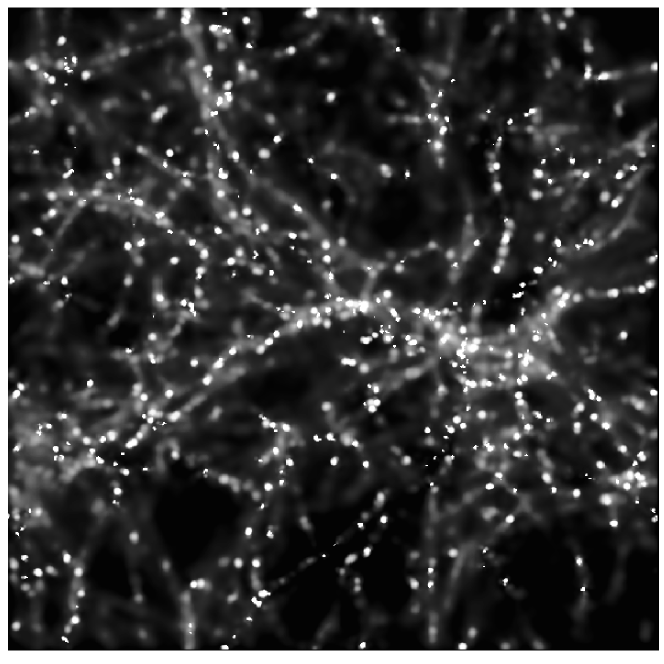
Figure 3 shows the spatial distribution of the gas in different regimes of density and temperature. Gas with $T<30,000\,{\rm K}$ and overdensity $\rho/\bar{\rho}<1000$ (upper left panel) mostly occupies the low density regions, though hints of the filaments in Figure 1 can be seen here as well. The filaments stand out dramatically in the warm gas component, with $30,000\,{\rm K}<T<10^{6}\,{\rm K}$ (upper right panel). This temperature cut selects gas that has been heated by adiabatic compression and mild shocks as it falls into moderate overdensity structures. The hottest gas ($T>10^{6}\,{\rm K}$, lower left panel) is confined to fully virialized dark matter potential wells, and its spatial distribution is more clumpy. The gas with $T<30,000\,{\rm K}$ and $\rho/\bar{\rho}>1000$ (lower right panel) occupies radiatively cooled knots inside these hot gas halos. The larger halos may contain several such knots. The most massive knots contain several hundred particles (merged into a single extended dot at the resolution of Figure 3), while the least massive, which are generally the ones that have started to cool and condense most recently, contain only a handful of cold gas particles. The gravitational softening of the simulation, 7 kpc at $z=2$, prevents us from resolving the detailed internal structure of these knots, but the physical conditions imply that they are likely to fragment and form stars. It is plausible to identify these knots as young — in some cases just forming — galaxies.

Knowing the density and temperature of each gas particle and the intensity of the model UV background, we can compute the corresponding neutral hydrogen fractions assuming ionization equilibrium. Figure 4 shows a 2-d map of the neutral hydrogen column density projected through the simulation cube. There is a close correspondence between the prominent structures in this map and the gas distributions in the right hand panels of Figure 3. The cold gas knots nearly always produce absorption at a column density of $N_{HI}=10^{17}\,{\rm cm}^{-2}$ or greater, features that appear white in the grey scale representation of Figure 4 (these regions are corrected for self-shielding using a procedure described in KWHM). The warm gas filaments produce the extended, lacy structures at lower column density. It is important to note that the faintest visible structures in Figure 4 have $N_{HI}\approx 10^{14.5}\,{\rm cm}^{-2}$, so much of the absorption at column densities typical of the Ly$\alpha$ forest arises in regions that are black in this Figure.

Figure 5.  : Examples of artificial spectra at $z=2$. Solid lines show transmission against velocity along four random lines of sight. At this redshift, the physical size of the periodic simulation box is 7.41 Mpc, corresponding to a Hubble flow of 1924.5 km/s. Dashed and dotted lines show spectra along lines of sight displaced arbitrarily from that of the primary spectrum by physical separations of 100 kpc and 300 kpc, respectively. The translation from velocity $v$ to wavelength $\lambda$ is $\lambda=1216\times(1+z)\times(1+v/c)$ Å, where $z=2$.

Figure 6.  : Distribution of neutral hydrogen column densities. The solid line shows the simulation results at $z=2$. Points with error bars are taken from the observational compilation by Petitjean et al. (1993).

Figure 5 shows artificial QSO absorption spectra along four randomly chosen lines of sight through the simulation box at $z=2$. In each panel, the solid line shows the transmission $T=e^{-\tau}$, where $\tau$ is the Ly$\alpha$ optical depth. The dashed line shows a spectrum along a line of sight 100 kpc away from this primary spectrum. The dotted line shows a spectrum at 300 kpc separation (200 kpc from the dashed spectrum). Many absorption features appear in both of the first two spectra, and there are significant matches even for lines of sight separated by 300 kpc, though these are often accompanied by substantial changes in the features’ depth or shape. Figure 4 shows that the low column density absorbing structures are extended and coherent, so the correlation of features along neighboring lines of sight is not surprising. Qualitatively, it appears that our results can account for the large coherence scale found in absorption studies of QSO pairs (e.g. Bechtold et al. 1994; Dinshaw et al. 1994, 1995), though quantitative tests (e.g. Charlton et al. 1995) are needed to assess the agreement or lack of agreement with recent observations.

Figure 6 displays the distribution of neutral hydrogen column densities, $d^{2}N/dN_{HI}\,dz$, at $z=2$. The procedure adopted to identify lines at column densities $N_{HI}<10^{15.5}\,{\rm cm}^{-2}$ is described in HKWM. Above this column density, we determine the distribution by measuring the fractional area above each column density in the projected HI map of Figure 4. High column density lines are rare enough that the absorption along any line of sight that has $N_{\rm HI}>10^{15.5}\,{\rm cm}^{-2}$ through our 7.4 Mpc box is always dominated by a single absorber. Observational data and error bars in Figure 6 are taken from Table 2 of Petitjean et al. Petitjean et al. (1993). There is a significant (factor of ten) discrepancy with the Petitjean et al. data for column densities near $10^{17}{\rm cm}^{-2}$, which could reflect either a failure of standard CDM or the presence in the real universe of an additional population of Lyman-limit systems that are not resolved by the simulation. Nonetheless, given that CDM is an a priori theoretical model that was not “designed” or adjusted to fit these observations, the overall level of agreement across eight orders of magnitude in neutral hydrogen column density is rather remarkable. Other analyses of absorption in this simulation are presented by HKWM and KWHM.

Cen et al. Cen et al. (1994), who were the first to use these sorts of simulations to model the Ly$\alpha$ forest, report similar agreement between observations and a low-$\Omega$ CDM model with a cosmological constant. Zhang et al. Zhang et al. (1995) find similar agreement for an $\Omega=1$ CDM model with a higher normalization ($\sigma_{8h^{-1}{\rm Mpc}}=1$) than used here. The qualitative success of three different models (and numerical methods) suggests that the Ly$\alpha$ forest arises naturally, and at least somewhat generically, in a hierarchical theory of structure formation with a photoionizing background. The comparison between simulations and the extraordinary data emerging from high resolution QSO spectra can clearly be carried out much more carefully than has been done so far. There is every reason to hope that detailed comparisons will reveal discrepancies that restrict the pool of acceptable theoretical models. For now, the agreement between simulated and observed line populations suggests that the simulation described here is worth taking seriously as a realistic general picture for the origin of Ly$\alpha$ absorbers.

In this simulation, the structures that produce low column density absorption ($N_{\rm HI}\sim 10^{13}-10^{15}{\rm cm}^{-2}$) are physically diverse: they include filaments of warm gas, caustics in frequency space produced by converging velocity flows McGill (1990), high density halos of hot, collisionally ionized gas, layers of cool gas sandwiched between shocks Cen et al. (1994), and modest local undulations in undistinguished regions of the intergalactic medium. Temperatures of the absorbing gas range from below $10^{4}K$ to above $10^{6}K$. The “typical” low column density absorbers — to the extent that we can identify such a class — are flattened structures of rather low overdensity ($\rho/\bar{\rho}\sim 1-10$), and their line widths are often set by peculiar motions or Hubble flow rather than thermal broadening. Because of their low overdensities, most of the absorbers are far from dynamical or thermal equilibrium, and many are still expanding with residual Hubble flow. The simulation reveals a smoothly fluctuating intergalactic medium, with no sharp distinction between “background” and “Ly$\alpha$ clouds”. Indeed, in this picture one might say that the Ly$\alpha$ forest is the absorption by diffuse intergalactic hydrogen known as the Gunn-Peterson Gunn and Peterson (1965) effect. There is also absorption by low density gas outside of the “lines,” but it is relatively weak. At higher redshifts, increasing neutral fractions make the absorbing gas more opaque, and the distinction between lines and background becomes even harder to draw.

A comparison between Figures 3 and 4 shows a clear association between high column density absorbers and the knots of radiatively cooled gas that represent forming galaxies. Damped Ly$\alpha$ absorption ($N_{\rm HI}\geq 10^{20.2}\,{\rm cm}^{-2}$) occurs along lines of sight that pass through the denser, more massive protogalaxies. The column density correlates inversely with the projected distance from the protogalaxy center, and the maximum projected separation that yields damped absorption is about 20 kpc (see KWHM). Lyman limit absorption ($10^{17}\,{\rm cm}^{-2}\leq N_{\rm HI}\leq 10^{20.2}\,{\rm cm}^{-2}$) occurs on lines of sight that pass either through the outer parts (20–100 kpc projected separation) of the more massive protogalaxies or near the centers of younger, lower density systems. By definition the stronger Lyman limit systems are self-shielded against the ionizing background, so they are mainly neutral, in constrast to the Ly$\alpha$ forest systems, which usually have neutral fractions of $10^{-6}-10^{-4}$.

3 Prospects for 21cm Observations

Figure 4 can be regarded as a (highly) idealized 21cm observation of a CDM universe at $z=2$, covering a region 15.1 arc-minutes on a side and 1924 km s^-1 in velocity. The contributions of Ingram and Braun to these proceedings show examples of what the Square-Kilometer Array (SKA) might see if it observed a universe like this, with realistic assumptions about resolution and noise. Here we will stick to more generic comments, inspired by the simulation but not directly tied to it. Some of the issues that affect the observability of high redshift HI in a variety of cosmological models are discussed by Scott and Rees Scott and Rees (1990) and references therein.

In a typical hierarchical model, the “re”combination of hydrogen at $z=1100$ is followed by an era of linear growth, with the density contrast of fluctuations $|\delta|\ll 1$ on all cosmologically relevant scales. To the extent that pressure and Compton drag against the microwave background can be ignored, density contrasts grow in proportion to the expansion factor, $\delta\propto a\propto t^{2/3}$. Once the strongest fluctuations (which occur on small scales) reach $\delta\sim 1$, they collapse, eventually giving rise to luminous objects that reionize the remaining diffuse gas. It is not at all clear what objects actually cause reionization (globular clusters? quasars? supermassive stars? dwarf galaxies?), but the visibility of high redshift quasars at wavelengths shorter than Ly$\alpha$ implies that the reionization occurred before $z\approx 5$. It could plausibly have happened much earlier (Tegmark et al., 1994; Fukugita and Kawasaki, 1994), though the detection of microwave background anisotropies at degree scales suggests that it did not occur at $z$ much above 50 Scott et al. (1995).

Reionization heats the diffuse medium to $T\sim 10^{4}\,{\rm K}$, introducing a Jeans mass — thermal pressure prevents baryons from collapsing into objects with circular velocities below about 35 km s^-1(Quinn et al., 1995; Thoul and Weinberg, 1995). Depending on the relative timing of reionization and fluctuation growth, the universe may enter a quiet phase during which little collapse occurs. Eventually, however, fluctuations larger than the Jeans mass reach the nonlinear regime, and the condensation of gas into protogalaxies and consequent star formation can begin in earnest. As time goes on and larger scale fluctuations become nonlinear, galaxies pull themselves into groups, clusters, and superclusters.

Reionization may have occurred at a redshift beyond the reach of current radio telescopes. However, it could have occurred at a redshift only slightly greater than 5, since at $z=5$ the density of quasars is plummeting and the opacity of the diffuse medium is rising. In this case, there might be interesting observables at $5<z<8$. Structure should be present on Mpc scales, and much of the gas should be cool enough to have a high neutral fraction. More work, including analysis of simulations, is needed to investigate whether the predicted structure is bright enough to detect with existing or plausible future instruments. If reionization takes place by the growth of “Stromgren spheres” around quasars or other rare objects, then there might be strong structure in the neutral hydrogen even where the underlying gas distribution is fairly uniform.

The prospects for HI emission searches above $z=5$ are intriguing but highly uncertain. Below this redshift, observations give more guidance about what to expect. In particular, we know that the universe is reionized, and the statistics of Ly$\alpha$ absorption give an estimate of the neutral hydrogen density parameter $\Omega_{HI}$.

In the simulation of §2, most of the gas at $z\sim 2-4$ is either in the low density, photoionized medium (roughly speaking, the Ly$\alpha$ forest), or in the high density, hot, collisionally ionized medium. However, nearly all of the neutral gas is in high density, radiatively cooled objects — Lyman limit and damped Ly$\alpha$ absorbers. This theoretical result is consistent with observational inferences, which show that the value of $\Omega_{HI}$ is dominated by contributions from the highest column density systems.

Single objects containing $10^{14}M_{\odot}$ of HI do not appear in the simulation, and they seem unlikely on generic grounds. The collapse of an object with $10^{14}M_{\odot}$ of baryons would shock–heat and collisionally ionize the gas, and before collapse the gas would be low density and photoionized. One could in principle have an object in which $10^{14}M_{\odot}$ of baryons collapsed and cooled — a sort of super damped Ly$\alpha$ system — but if such objects were common we would expect to see many galaxies with $10^{14}M_{\odot}$ of stars today.

The simulated observations of Ingram and Braun in these proceedings show that it is difficult to detect the faint caustics seen in Figure 4 even with an instrument as ambitious as the SKA. What the SKA can detect rather easily are the damped Ly$\alpha$ systems, which are more numerous than present day, $L^{*}$ galaxies by a factor of several. A single pointing covers a small angular field, but it is sensitive to a gigantic range in redshift. A program of multiple long exposures could thus provide a “galaxy” (damped Ly$\alpha$) redshift survey over a large cosmological volume at high redshift. This would be an extraordinary feat, and observing the history of galaxy clustering would doubtless teach us a great deal about the underlying physics of structure formation.

At lower sensitivity, the first objects to be detected in 21cm emission at high redshift are likely to be clusters of damped Ly$\alpha$ systems, the high redshift analogs of today’s rich galaxy clusters. The statistics of these can in principle be calculated from simulations, but very large simulation volumes are needed to predict the abundance of the rarest, most massive systems. We will therefore attempt a more phenomenological calculation, based on scaling the abundance of present galaxy clusters back to high $z$.

Bahcall and Cen Bahcall and Cen (1993) find that the abundance of observed rich clusters with total mass $M$ or greater can be described by the cumulative mass function

$$n(>M)=n_{0}^{*}(M/M_{0}^{*})^{-1}e^{-M/M_{0}^{*}},$$

with $M_{0}^{*}=1.8\times 10^{14}h^{-1}M_{\odot}$ and $n_{0}^{*}=4\times 10^{-5}h^{3}$ Mpc^-3. Suppose that this mass function has emerged from a hierarchical model of structure formation in which the power spectrum on the scales of interest can be approximated as $P(k)\propto k^{n}$. The characteristic mass $M_{0}^{*}$ corresponds to the scale on which the rms linear theory mass fluctuations have some value $\sigma^{*}\sim 1/2$, so that only the rare ($\sim 2-3\sigma$) fluctuations on this scale have collapsed to form virialized clusters. At high redshift we might expect a mass function of similar form, but the characteristic mass $M_{z}^{*}$ will correspond to the (smaller) scale on which the rms fluctuation is $\sigma^{*}$ at this redshift. For a $k^{n}$ power spectrum,

$$\sigma(M,z)=\sigma^{*}(M/M_{0}^{*})^{-(3+n)/6}D(z),$$

where a useful approximation to the growth factor $D(z)$ is Shandarin et al. (1983)

$$D(z)\approx\left(1+{2.5\Omega_{0}z\over 1+1.5\Omega_{0}}\right)^{-1}.$$

The condition $\sigma(M_{z}^{*},z)=\sigma^{*}$ implies that the characteristic mass at redshift $z$ is $M_{z}^{*}=M_{0}^{*}D^{6/(3+n)}.$ The abundance $n_{z}^{*}$, in comoving units, can be determined from the condition $n_{z}^{*}M_{z}^{*}=n_{0}^{*}M_{0}^{*}\Longrightarrow n_{z}^{*}=n_{0}^{*}D^{-6/(3+n)}$, since objects of mass $M>M^{*}$ contain a constant fraction of the total mass of the universe in this sort of scale free model.

For our purposes, we are interested in a cluster’s HI mass rather than its total mass. To go from one to the other, we can make the adventurous assumption that the ratio of $M_{HI}$ to $M_{tot}$ is the same as the universal ratio $\Omega_{HI}(z)/\Omega(z)$. This assumption is almost certainly incorrect today because the galaxies in clusters tend to be gas poor, early types. It may be more plausible at high redshift, when galaxies are primarily gaseous; indeed, the error may be in the opposite sense (underestimating $M_{HI}$ instead of overestimating) if galaxies at high $z$ formed preferentially in the densest regions. Putting all of this together, we arrive at an expression for the cumulative, comoving number density of clusters with HI mass greater than $M_{HI}$:

$$n(>M_{HI})=n_{0}^{*}F\left({M_{HI}F\over RM_{0}^{*}}\right)^{-1}{\rm exp}\left({-M_{HI}F\over RM_{0}^{*}}\right)~{},$$

$$M_{0}^{*}=1.8\times 10^{14}h^{-1}M_{\odot},\quad n_{0}^{*}=4\times 10^{-5}h^{3}{\rm\ comoving\ Mpc}^{-3},$$

$$F\equiv D^{-6/(3+n)},\quad R\equiv{\Omega_{HI}(z)\over\Omega(z)}={\Omega_{HI}(z)\over\Omega_{0}}{(1+\Omega_{0}z)\over(1+z)}~{}.$$

There are many ways that this calculation could depart from reality, but it illustrates how the power spectrum, the cosmological model, and the history of the neutral gas density might interact in determining the abundance of observable high redshift objects. Unfortunately, the numbers that it yields are not particularly encouraging because even today the HI mass of an $M^{*}$ object is only several$\,\times\,10^{11}h^{-1}M_{\odot}$, and at higher redshift the tendency of galaxies to be more gas rich is countered by the lower masses of the largest collapsed clusters. As a specific example, if we adopt $z=3$, $n=-1$, $\Omega_{0}=0.3$, and $\Omega_{HI}(z)=0.004$, then $F=16.61$, $R=6.3\times 10^{-3}$, the HI mass of an $M^{*}$ object is $RM_{0}^{*}F^{-1}=6.9\times 10^{10}h^{-1}M_{\odot}$, and the abundance of such objects is $n_{0}^{*}Fe^{-1}=2.4\times 10^{-4}\,h^{3}$ comoving Mpc^-3. For an HI mass of $3\times 10^{11}h^{-1}M_{\odot}$, 4.37 times higher, the abundance is down by a factor of $e^{-4.37}/4.37$ to $6.9\times 10^{-7}h^{3}$ comoving Mpc^-3.

Of course, the fact that this argument leads to a low abundance of massive HI concentrations means that detection of such a concentration would be all the more interesting. The most dubious elements of the argument (if one is looking for order of magnitude gains, not factors of 2) are probably the assumption that the HI to total mass ratio $R$ is universal and the assumption that the objects easiest to detect are indeed collapsed clusters as opposed to, e.g., lower overdensity structures that are just detaching from the Hubble flow.

4 Conclusions

According to conventional theories of cosmic structure fomration, the large scale structure that we observe today should be mirrored in a scaled down form at high redshift. Absorption and emission measurements of high redshift HI can trace out the elements of this small scale structure. The agreement between hydrodynamic simulations and observed quasar spectra suggests that the Ly$\alpha$ forest is produced largely by the moderately overdense ($\rho/\bar{\rho}\sim 1-10$) components of this structure, especially the collapsing filaments and sheets of warm, photoionized gas. Lyman limit and damped Ly$\alpha$ absorption probably arises in the radiatively cooled gas of forming galaxies. Detecting 21cm emission from high redshifts is an ambitious goal, but simulated observations and inferences from absorption suggest that the radio arrays of the future could map the youthful universe in the way that today’s galaxy redshift surveys have mapped the local large scale structure. The opportunity to watch galaxies, clusters, voids, and superclusters grow through time should take us a long way towards understanding their origin in the physics of the big bang.

DW acknowledges research and travel support from NASA grant NAG5-2882.

References

- Bechtold et al. (1994) Bechtold, J., Crotts, A.P.S., Duncan, R.C. and Fang, Y. (1994), ApJ, 437, L83
- Bahcall and Cen (1993) Bahcall, N. A. and Cen, R. (1993), ApJ, 407, L49
- Bunn et al. (1995) Bunn, E. F., Scott, D., and White, M. (1995), ApJ, 441, L9
- Cen et al. (1994) Cen, R., Miralda-Escudé, J., Ostriker, J.P. and Rauch, M. (1994), ApJ, 437, L9
- Charlton et al. (1995) Charlton, J.C., Churchill, C.W., and Linder, S.M. (1995), ApJ, 452, L81
- Dinshaw et al. (1995) Dinshaw, N., Foltz, C.B., Impey, C.D., Weymann, R.J. and Morris, S.L. (1995), Nature, 373, 223
- Dinshaw et al. (1994) Dinshaw, N., Impey, C.D., Foltz, C.B., Weymann, R.J. and Chaffee, F.H. (1994), ApJ, 437, L87
- Fukugita and Kawasaki (1994) Fukugita, M. and Kawasaki, M. (1994), MNRAS, 269, 563
- Gunn and Peterson (1965) Gunn, J.E. and Peterson, B.A. (1965), ApJ, 142, 1633
- Hernquist et al. (1995) Hernquist, L., Katz, N., Weinberg, D. H. and Miralda-Escudé, J. (1995), submitted to ApJ Letters (HKWM)
- Katz et al. (1995a) Katz, N., Weinberg, D. H. and Hernquist, L. (1995), submitted to ApJS
- Katz et al. (1995b) Katz, N., Weinberg, D. H., Hernquist, L. and Miralda-Escudé, J. (1995), submitted to ApJ Letters (KWHM)
- McGill (1990) McGill, C. (1990), MNRAS, 242, 544
- Melott and Shandarin (1993) Melott, A. L. and Shandarin, S. F. (1993), ApJ, 410, 469
- Petitjean et al. (1993) Petitjean, P., Webb, J.K., Rauch, M., Carswell, R.F. and Lanzetta, K. 1993, MNRAS, 262, 499
- Quinn et al. (1995) Quinn, T., Katz, N., and Efstathiou, G. (1995), MNRAS, in press
- Scott and Rees (1990) Scott, D. and Rees, M. J. (1990), MNRAS, 247, 510
- Scott et al. (1995) Scott, D., Silk, J., and White, M. (1995), Science, 268, 829
- Shandarin et al. (1983) Shandarin, S. F., Doroshkevich, A. G., and Zel’dovich, Ya. B (1983), Sov Phys Usp, 26, 46
- Shandarin and Zel’dovich (1989) Shandarin, S. F. and Zel’dovich, Ya. B (1993), Rev Mod Phys, 61, 185
- Tegmark et al. (1994) Tegmark, M., Silk, J., and Blanchard, A. (1994), ApJ, 420, 2
- Thoul and Weinberg (1995) Thoul, A. A. and Weinberg, D. H. (1995), submitted to ApJ
- Weinberg and Gunn (1990) Weinberg, D. H. and Gunn, J. E. (1990), MNRAS, 247, 260
- White et al. (1993) White, S. D. M., Efstathiou, G., and Frenk, C. S. (1993), MNRAS, 262, 1023
- Zel’dovich (1970) Zel’dovich, Y. B. 1970, A&A, 5, 84
- Zhang et al. (1995) Zhang, Y., Anninos, P. & Norman, M.L. 1995, preprint astro-ph/9508133