Abstract

Modeling the atmospheres of SNe Ia requires the solution of the NLTE radiative transfer equation. We discuss the formulation of the radiative transfer equation in the co-moving frame. For characteristic velocities larger than $\sim 2000$ km s^-1, the effects of advection on the synthetic spectra are non-negligible, and hence should be included in model calculations. We show that the time-independent or quasi-static approximation is adequate for SNe Ia near maximum light, as well as for most other astrophysical problems; e.g., hot stars, novae, and other types of supernovae. We examine the use of the Sobolev approximation in modeling moving atmospheres and find that the number of overlapping lines in the co-moving frame make the approximation suspect in models that predict both lines and continua. We briefly discuss the form of the Rosseland mean opacity in the co-moving frame, and present a formula that is easy to implement in radiation hydrodynamics calculations.

1 Introduction

There are many astrophysical systems that require a solution to the radiative transfer equation in moving media; e.g., Wolf-Rayet and other hot stars with stellar winds, novae, supernovae, the material surrounding quasars, and even the early phases of the universe when the material is still optically thick (?). Because there is such a large simplification in the radiation-matter interaction terms, it is both customary and expedient to solve the radiation transfer equation in the co-moving frame. In a series of papers Mihalas and co-workers (?????) examined methods for solving the co-moving frame line-transfer problem, where the Doppler effect dominates because the characteristic width over which the line profile varies is small. This effectively increases the importance of the Doppler effect over the other $O(v/c)$ (advection and aberration) effects by the ratio $c/v_{\rm therm}$, where $v_{\rm therm}$ is the thermal velocity corresponding to the intrinsic Doppler line-width. Recently, there have been increasingly sophisticated attempts to model the atmospheres of hot stars (e.g., ?), novae (??), and supernovae (?????), including NLTE for lines and continua, and the effects of line blanketing. Here we systematically discuss the important effects that must be included when solving the radiative transfer equation in the co-moving frame, elucidate the range of applicability of Eulerian approximations such as the Sobolev approximation, and present a co-moving formulation of the Rosseland mean opacity. Some of the results discussed here are also discussed in ?).

2 Radiative Transfer Equation

The co-moving frame radiative transfer equation for spherically symmetric flows can be written as (cf. ?):

$$\gamma(1+\beta\mu)\frac{\partial{I_{\nu}}}{\partial t}+\gamma(\mu+\beta)\frac{\partial{I_{\nu}}}{\partial r}$$

$$+ \frac{\partial}{\partial\mu}\left\{\gamma(1-\mu^{2})\left[\frac{1+\beta\mu}{r}\right.\right.$$

$$\left.\left.\quad-\gamma^{2}(\mu+\beta)\frac{\partial\beta}{\partial r}-\gamma^{2}(1+\beta\mu)\frac{\partial\beta}{\partial t}\right]{I_{\nu}}\right\}$$

$$- \frac{\partial}{\partial\nu}\left\{\gamma\nu\left[\frac{\beta(1-\mu^{2})}{r}+\gamma^{2}\mu(\mu+\beta)\frac{\partial\beta}{\partial r}\right.\right.$$

$$\left.\left.\quad+\gamma^{2}\mu(1+\beta\mu)\frac{\partial\beta}{\partial t}\right]{I_{\nu}}\right\}$$

$$+ \gamma\left\{\frac{2\mu+\beta(3-\mu^{2})}{r}\right.$$

$$\quad\left.+\gamma^{2}(1+\mu^{2}+2\beta\mu)\frac{\partial\beta}{\partial r}+\gamma^{2}[2\mu+\beta(1+\mu^{2})]\frac{\partial\beta}{\partial t}\right\}{I_{\nu}}$$

$$=\eta_{\nu}-\chi_{\nu}{I_{\nu}}.$$

We set $c=1$; $\beta$ is the velocity; and $\gamma=(1-\beta^{2})^{-1/2}$ is the usual Lorentz factor. We emphasize that, in Eq. 2, the physical (dependent) variables are all evaluated in the co-moving Lagrangian frame. However, the choice of independent variables is free, and the coordinate $r$ in Eq. 2 is an Eulerian variable (for a discussion of this point, cf. ?). This is the most convenient choice for solving the transfer equation, where one usually specifies the grid by fixing the optical depth for some reference frequency. However, this grid differs from the fully Lagrangian grid typically used in radiation hydrodynamics. In the latter case, $r\equiv r(m)$.

In order to illuminate the physics, and without loss of generality, we expand Eq. 2 in powers of $\beta$ and keep terms only to $O(\beta)$. While this is not necessary (???), it is adequate for most astrophysical flows. To $O(\beta)$, the radiation transport equation becomes:

$$\frac{\partial{I_{\nu}}}{\partial t}+(\mu+\beta)\frac{\partial{I_{\nu}}}{\partial r}$$

$$+(1-\mu^{2})\left[\mu(\frac{\beta}{r}-\frac{\partial\beta}{\partial r})+\frac{1}{r}-\frac{\partial\beta}{\partial t}\right]\frac{\partial{I_{\nu}}}{\partial\mu}$$

$$+\left[\mu^{2}(\frac{\beta}{r}-\frac{\partial\beta}{\partial r})-\frac{\beta}{r}\right]\left\{\frac{\partial{I_{\nu}}}{\partial\ln\nu}-3{I_{\nu}}\right\}-\mu\frac{\partial\beta}{\partial t}\frac{\partial{I_{\nu}}}{\partial\ln\nu}$$ (2)

$$=\eta_{\nu}-\chi_{\nu}{I_{\nu}}.$$

In writing Eq. 2, we have retained the first term, which accounts for the explicit time dependence of the radiation field in the co-moving frame. We have also retained the acceleration term, $\frac{\partial\beta}{\partial t}$. Both terms are of $O(\beta)$ when compared to other terms in the equation, such as the $\beta/r$ terms, and hence, are of $O(\beta^{2})$ on a fluid flow timescale and can be dropped (????). Upon doing so, one derives the time-independent (or quasi-static) transfer equation in the co-moving frame:

$$(\mu+\beta)\frac{\partial{I_{\nu}}}{\partial r}+(1-\mu^{2})\left[\mu(\frac{\beta}{r}-\frac{\partial\beta}{\partial r})+\frac{1}{r}\right]\frac{\partial{I_{\nu}}}{\partial\mu}$$ (3)

$$+\left[\mu^{2}(\frac{\beta}{r}-\frac{\partial\beta}{\partial r})-\frac{\beta}{r}\right]\left\{\frac{\partial{I_{\nu}}}{\partial\ln\nu}-3{I_{\nu}}\right\}$$

$$=\eta_{\nu}-\chi_{\nu}{I_{\nu}}.$$

To further simplify the equation and to help elucidate the fundamental physics, let us restrict ourselves to consideration of homologous flows: $\beta\propto r$. In this case Eq. 3 becomes:

$$(\mu+\beta)\frac{\partial{I_{\nu}}}{\partial r}+\frac{(1-\mu^{2})}{r}\frac{\partial{I_{\nu}}}{\partial\mu}-\frac{\beta}{r}\left\{\frac{\partial{I_{\nu}}}{\partial\ln\nu}-3{I_{\nu}}\right\}$$ (4)

$$=\eta_{\nu}-\chi_{\nu}{I_{\nu}}.$$

In order to identify the physical significance of the terms, it is useful to compare this equation to its static counterpart:

$$\mu\frac{\partial{I_{\nu}}}{\partial r}+\frac{(1-\mu^{2})}{r}\frac{\partial{I_{\nu}}}{\partial\mu}=\eta_{\nu}-\chi_{\nu}{I_{\nu}}.$$ (5)

Comparing Eqs. 4 and 5, the physical meaning of the terms is apparent: $\beta\frac{\partial{I_{\nu}}}{\partial r}$ is the advection term, ${\beta}/{r}\frac{\partial{I_{\nu}}}{\partial\ln\nu}$ represents the Doppler shift, and $-3\beta/r{I_{\nu}}$ describes the effect of aberration.

It is clear that all three terms are of O($\beta$) and must be retained to have a consistent treatment in the co-moving frame. The $O(\beta)$ transport equation is more difficult to solve because the characteristics, which are simply parallel lines of constant impact parameter when the advection term, $\beta\frac{\partial{I_{\nu}}}{\partial r}$, is neglected, become curved lines; therefore, the reflection symmetry is lost (??). This is because the material is moving, “sweeping up” radiation, causing the characteristics to be curved. Therefore, one can no longer use reflection symmetry to integrate the solution only along outgoing rays. One must integrate along both incoming and outgoing rays (???). ?) examined the magnitude of the advection and aberration terms and estimated that they are of order $5\beta$ and that the advection term is more important than the aberration term.

Let us now examine the moments of Eq. 4. The zeroth moment is:

$$\beta\frac{\partial{J_{\nu}}}{\partial r}+\frac{1}{r^{2}}\frac{\partial(r^{2}{H_{\nu}})}{\partial r}+\frac{\beta}{r}(3{J_{\nu}}-\frac{\partial{J_{\nu}}}{\partial\ln\nu})=\eta_{\nu}-\chi_{\nu}{J_{\nu}},$$ (6)

and the first moment is:

$$\frac{\partial{K_{\nu}}}{\partial r} + \frac{\beta}{r^{2}}\frac{\partial(r^{2}{H_{\nu}})}{\partial r}-\frac{({J_{\nu}}-3{K_{\nu}})}{r}+\frac{\beta}{r}({H_{\nu}}-\frac{\partial{H_{\nu}}}{\partial\ln\nu})$$ (7)

$$= -\chi_{\nu}{H_{\nu}}.$$

The Eddington moments are given by:

$$J_{\nu} = \frac{1}{2}\int_{-1}^{1}{I_{\nu}}\,d\mu$$

$$H_{\nu} = \frac{1}{2}\int_{-1}^{1}\mu{I_{\nu}}\,d\mu$$ (8)

$$K_{\nu} = \frac{1}{2}\int_{-1}^{1}\mu^{2}{I_{\nu}}\,d\mu$$

where $\mu=\cos\theta$. When advection is neglected, the moment equations become:

$$\displaystyle\frac{1}{r^{2}}\frac{\partial(r^{2}{H_{\nu}})}{\partial r} +\frac{\beta}{r}(3{J_{\nu}}-\frac{\partial{J_{\nu}}}{\partial\ln\nu})=\eta_{\nu}-\chi_{\nu}{J_{\nu}},$$

$$\displaystyle\frac{\partial{K_{\nu}}}{\partial r} -\frac{({J_{\nu}}-3{K_{\nu}})}{r}+\frac{\beta}{r}(3{H_{\nu}}-\frac{\partial{H_{\nu}}}{\partial\ln\nu})$$

$$= -\chi_{\nu}{H_{\nu}},$$ (10)

i.e., the gradient of the energy density is absent from the zeroth moment equation, and the divergence of the flux is no longer included in the first moment equation. Integrating the moment equations (Eqs. 6 and 7) over frequency, and assuming that radiative equilibrium holds, i.e., that energy is conserved or total emission equals total absorption [$\int_{0}^{\infty}(\eta_{\nu}-\chi_{\nu}{J_{\nu}})\,d\nu=0$], one obtains for the zeroth moment:

$$\frac{D\,J}{D\,t}+\frac{1}{r^{2}}\frac{\partial(r^{2}\,H)}{\partial r}+\frac{4\beta}{r}J=0,$$ (11)

where we have restored the time derivative:

$$\frac{D}{Dt}=\frac{\partial}{\partial t}+\beta\frac{\partial}{\partial r}.$$ (12)

It has been suggested (?) that one can correct for neglecting the advection term and include the effects of the radiation field time dependence on a radiation flow timescale by using Eq. 11 and by arbitrarily setting the co-moving luminosity ($=r^{2}\,H$) to be constant. In this case, Eq. 11 becomes:

$$\frac{D\,J}{D\,t}=-\frac{4\beta}{r}J.$$ (13)

This is interpreted as an operator equality:

$$\frac{D}{Dt}=-\frac{4\beta}{r}.$$ (14)

When Eq. 14 is substituted into the radiation transport equation, the transport equation becomes:

$$\mu\frac{\partial{I_{\nu}}}{\partial r}+\frac{(1-\mu^{2})}{r}\frac{\partial{I_{\nu}}}{\partial\mu}-\frac{\beta}{r}\left\{\frac{\partial{I_{\nu}}}{\partial\ln\nu}+{I_{\nu}}\right\}=\eta_{\nu}-\chi_{\nu}{I_{\nu}}.$$ (15)

Comparing Eq. 15 to Eq. 4, we see that this scheme is equivalent to making the quasi-static approximation, neglecting advection, and changing the sign and coefficient of the aberration term, which is unphysical.

We have compared simulations with and without the advection term for two models that provide reasonable fits to SN 1987A at 13 and 31 days after explosion. These calculations were performed using version 5.5.9 of the general radiative transfer code, PHOENIX, developed by Hauschildt (???). This code accurately solves the fully relativistic transfer equation, Eq. 2, in the quasi-static approximation, $\frac{\partial{I_{\nu}}}{\partial t}=0$ (Note contrary to what is incorrectly stated by Höflich et al., in this volume, we do not solve a simple non-relativistic transport equation with the Rybicki method, but we indeed solve the full special relativistic, spherically symmetric radiative transfer equation for lines and continua with an operator splitting scheme based on a short characteristic method with non-local, adjustable approximate $\Lambda$-operator). The model parameters are given in Table 1 (for a discussion of the model parameters, cf. ?). For the day-13 spectrum, Figure 1 compares the spectra of a calculation that includes advection with one that does not, while Figure 2 displays the same for day-31. The differences are about the size predicted by ?), with the effects being more apparent in the faster day-13 model than in the much slower day-31 model. Figures 3 and 4 show comparisons of the temperature profiles for both models. Neglecting advection alters the temperature structure, which can be interpreted as resulting from the change in the relations between the moments (compare Eqs. 6 and 7 with Eqs. 2 and 10). Figure 5 illustrates that this is the most important effect of neglecting advection. The temperature structure and departure coefficients are kept fixed in order to only alter the transport equation. In this case, the emergent spectra are much more similar than those in Fig. 1. From these results, it is clear that the effects of advection should not be neglected in models of supernovae where the characteristic velocities are larger than $\approx 5000$ km s^-1. For systems where velocities are lower than $\sim 2000$ km s^-1, advection may be neglected with reasonable accuracy.

Day 13 Day 31   $T_{\rm eff}$ (K) 5400 4400 $v_{0}$ (km s^-1) 5500 1700 $R_{0}$ (cm) $6.1\times 10^{14}$ $4.5\times 10^{14}$ N 6 6

TABLE 1.  : ${T_{\rm eff}}$, $R_{0}$ , ${v_{0}}$ are the “effective” temperature, radius, and velocity at the reference point $\tau_{\rm std}=1$; N is the power-law density index.

Figure 1.  : The spectrum produced by a full calculation, which fit SN 1987A at 13 days past explosion (solid line), is compared to one with the same parameters in which advection is neglected (dot-dashed line). Both calculations are in radiative equilibrium.

Figure 2.  : The spectrum produced by a full calculation, which fit SN 1987A at 31 days past explosion (solid line), is compared to one with the same parameters in which advection is neglected (dot-dashed line). Both calculations are in radiative equilibrium.

Figure 3.  : The temperature profiles for the models plotted in Fig. 1 are compared.

Figure 4.  : The temperature profiles for the models plotted in Fig. 2 are compared.

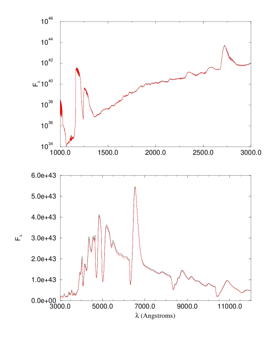
Figure 5.  : The spectrum produced by a full calculation, which fit SN 1987A at 13 days past explosion (solid line), is compared to one with the same parameters in which advection is neglected (dotted line). The structure is fixed to be that of the full calculation.

3 Quasi-Static Approximation

We can estimate the effects of making the quasi-static approximation by examining the radiation transfer equation. For clarity, we again restrict ourselves to $O(\beta)$ and homologous flows. Restoring the time derivative in Eq. 4, we have:

$$\frac{\partial{I_{\nu}}}{\partial t} + (\mu+\beta)\frac{\partial{I_{\nu}}}{\partial r}+\frac{(1-\mu^{2})}{r}\frac{\partial{I_{\nu}}}{\partial\mu}$$ (16)

$$- \frac{\beta}{r}\left\{\frac{\partial{I_{\nu}}}{\partial\ln\nu}-3{I_{\nu}}\right\}$$

$$=\eta_{\nu}-\chi_{\nu}{I_{\nu}}.$$

In order to solve this equation numerically, we would replace the time derivative with the difference:

$$\frac{\partial{I_{\nu}}}{\partial t}=\frac{{I_{\nu}}-{I_{\nu}}^{n}}{\delta t},$$ (17)

where ${I_{\nu}}^{n}$ is the intensity evaluated at the previous time $t^{n}$, ${I_{\nu}}$ is the intensity at the current time $t^{n+1}$, and $\delta t=t^{n+1}-t^{n}$. Inserting this expression into Eq. 16, and moving the time derivative to the right-hand side of the transfer equation, we obtain:

$$(\mu+\beta)\frac{\partial{I_{\nu}}}{\partial r} + \frac{(1-\mu^{2})}{r}\frac{\partial{I_{\nu}}}{\partial\mu}-\frac{\beta}{r}\left\{\frac{\partial{I_{\nu}}}{\partial\ln\nu}-3{I_{\nu}}\right\}$$ (18)

$$= (\eta_{\nu}+\frac{{I_{\nu}}^{n}}{\delta t})-(\chi_{\nu}+\frac{1}{\delta t}){I_{\nu}},$$

which shows that the time derivative term can be viewed as an additional source and sink of radiation. We can estimate the size of the error made in the quasi-static approximation by examining the ratio $\chi^{-1}/(c\delta t)$, where we have restored the explicit $c$. In supernovae, the natural timescale is the age of the object, $t=R/v$. We may estimate that $\chi\approx\tau/R$, where $\tau$ is an appropriate optical depth. Then, the ratio becomes:

$$\frac{\chi^{-1}}{c\delta t}\approx\frac{\beta}{\tau}.$$ (19)

For Type Ia supernovae at maximum light, the continuum extinction optical depth is about 10, and $\beta\sim 1/30$. So the error is at most 0.3%; small compared to errors in the atomic physics. This error will be considerably smaller for other types of supernovae, which are optically thick for longer times. In fact, Eq. 19 is an overestimate of the error because we have neglected the source term ${I_{\nu}}^{n}/(c\delta t)$, which counteracts the extra sink term.

Claims (Eastman, this volume) that in order to account for “old photons”, time dependence must be included in the transfer equation are not correct. The effects of both dynamic and static diffusion are included in radiation hydrodynamics without including the time-dependent term in the transfer equation (?). The effects of departures from radiative equilibrium can be included in our modeling.

4 NLTE Effects

Figure 6 displays the model atoms for Li I, Ca II, Ti I, Ti II, Fe II, and Co II used in PHOENIX. In addition H I, He I, He II, Mg II, Ne I, and O I are also treated in NLTE. In the very near future we will add C I-IV, N I-VI, O II–VI, Si II–III, and S II–III. In particular, our large Fe II model atom (617 levels, 13675 primary transitions; see ?, for more details) allows us to determine the importance of the size of model atoms and of the validity of common assumptions that are often made in handling the millions of secondary transitions that must be included in order to correctly reproduce the UV line blanketing. We find that large changes in luminosity (see Pinto, this volume) can be avoided by treating the secondary lines with a small but non-zero thermalization parameter (?), as required by physical considerations.

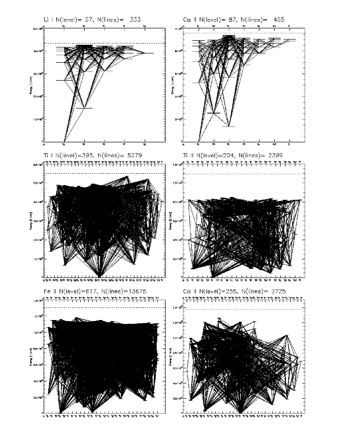
Figure 6.  : Grotrian diagrams for Li I, Ca II, Ti I, Ti II, Fe II, and Co II model atoms used in the calculations. Only the “primary” radiative transitions are displayed; see ?) and ?) for more details.

5 Sobolev Approximation

The Sobolev approximation developed by ?) and ?) and extended by ??) and ????) has proven extremely valuable in providing line identifications and minimum and maximum velocities in supernovae (????????), because it allows one to calculate line profiles without solving the transfer equation, it is nearly analytic, and quite convenient. The above analyses were concerned with identifying strong lines, and continuum effects were neglected. More recently the Sobolev approximation has been used to solve the rate equations for detailed model atoms including continua (??, Höflich et al., this volume). However, because the escape probability is derived by neglecting the effects of neighboring lines, it is only valid for isolated lines, and is invalid when there are many weak overlapping lines (???). This is likely to be the case in the UV, where line blanketing is severe. ?) also has discussed that escape probability methods such as the Sobolev approximation are inaccurate at small line optical depths, particularly when there are many overlapping lines. Since the source function predicted by the Sobolev approximation at the surface is incorrect by a factor of $\sqrt{\epsilon}$, where $\epsilon$ is the line thermalization parameter, the value of $J$ found by the formal solution will also be in error, which in turn will lead to errors in the rate equations. In Figure 7 we display the number of overlapping lines in a range of 6 intrinsic Doppler widths around any given wavelength, as a function of wavelength, for the day-13 SN 1987A model, which has a statistical or micro-turbulent velocity of $\xi=50$ km s^-1. The lines are said to overlap if, for any particular line, another line has its line center $\pm 6$ intrinsic line-widths from the reference line. The Doppler widths are calculated at deepest depth point in the model. As expected, in the UV the mean number of overlapping lines is typically around 100, and can be as large as 500. This implies that the radiative transfer in SN (and nova) atmospheres must explicitly include the effects of overlapping lines and continua. Otherwise, the radiative rates for these transitions would be incorrect, particularly in the outer parts of the atmosphere where ionization corrections are most important. Although this requires a very fine wavelength grid for the model calculations, detailed models can be computed using modern numerical techniques on even moderately sized workstations. Thus, the Sobolev approximation cannot be used in detailed NLTE calculations for SNe, because the radiative rates calculated in this approximation are inaccurate. Similar results have been obtained by ?) in nova model atmosphere calculations.

Figure 7.  : The number of overlapping lines in a range of 6 Doppler widths around any given wavelength, as a function of wavelength, for the day-13 SN 1987A model. Only lines stronger than $10^{-3}$ times the local b-f continuum are included. Clearly, the Sobolev assumption that individual lines do not overlap is not fulfilled.

For pure hydrogen atmospheres, ?) found good agreement between the non-relativistic Sobolev approximation and non-relativistic co-moving frame full transport calculations, which shows that the Sobolev approximation is accurate for well separated lines such as the Balmer lines. However, this situation is not reproduced in most spectral regions, and therefore, the Sobolev approximation is of limited use for detailed modeling of SN or nova envelopes.

6 Expansion Opacities

Radiation hydrodynamic calculations of supernova light curves require accurate fluxes, and it has long been realized that the static Rosseland mean opacity does not produce an accurate flux in moving atmospheres (?). The work of ?) provided an approximate formula for the Rosseland mean opacity in the observer’s frame. However, nearly all radiation hydrodynamics calculations are performed in the co-moving frame; hence, a co-moving formulation is required.

We have derived the Rosseland mean opacity in the co-moving frame to $O(\beta)$ (?). Let us first recall that the static Rosseland mean, $\chi_{R}^{0}$, is given by:

$$\frac{1}{\chi_{R}^{0}}=(4\frac{\sigma}{\pi}T^{3})^{-1}\int_{0}^{\infty}\chi_{\nu}^{-1}\frac{dB_{\nu}}{dT}\,d\nu.$$ (20)

To derive the non-static Rosseland mean, we will assume homologous flows. In addition, we make the Eddington approximation, ${K_{\nu}}=1/3{J_{\nu}}$, implying that the co-moving radiation field is close to isotropic, which is an excellent approximation in the diffusive regime (large optical depth) because the radiation is collision dominated (?).

We find that the co-moving Rosseland mean opacity to $O(\beta)$ is given by:

$$\frac{1}{\chi_{R}^{\beta}}\equiv(\chi+\frac{2\beta}{r})^{-1}$$ (21)

in the gray case, and:

$$\frac{1}{\chi_{R}^{\beta}}=\mbox{\hskip 166.2212pt}$$

$$(4\frac{\sigma}{\pi}T^{3})^{-1}\int_{0}^{\infty}\chi_{\nu}^{-1}[1-\frac{\beta}{r\chi^{0}_{R}}(1-\frac{\partial}{\partial\ln\nu})]\frac{dB_{\nu}}{dT}\,d\nu,$$ (22)

$$=\frac{1}{\chi^{0}_{R}}\left[{1-\frac{\beta}{\chi^{0}_{R}r}+\frac{\beta}{r}(4\frac{\sigma}{\pi}T^{3})^{-1}\int_{0}^{\infty}\chi_{\nu}^{-1}\frac{\partial^{2}B_{\nu}}{\partial T\partial\ln\nu}\,d{\nu}}\right],$$ (23)

in the non-gray case. In deriving Eq. 23, we have used $\frac{\partial B}{\partial r}=4(\sigma/\pi)T^{3}\frac{\partial T}{\partial r}$.

It follows that the co-moving multi-group flux to be used in radiation hydrodynamics is given by a Fick’s law diffusion equation:

$$H_{\nu}^{\beta}=-\frac{1}{3\chi_{R}^{\beta}}\frac{\partial B_{\nu}}{\partial r}.$$ (24)

We emphasize that $\chi_{\nu}$ in Eq. 20 and 23 contains contributions from continua, lines, and scattering opacities, and nowhere have we had to treat lines differently from continua.

In the case that the opacity may be approximated by a power-law, $\chi_{\nu}\propto\nu^{-n}$, the last integral in Eq. 23 may be evaluated by an integration by parts, yielding:

$$\frac{\beta}{r}(4\frac{\sigma}{\pi}T^{3})^{-1}\int_{0}^{\infty}\chi_{\nu}^{-1}\frac{\partial^{2}B_{\nu}}{\partial T\partial\ln\nu}\,d{\nu}=-(n+1)\frac{\beta}{r\chi^{0}_{R}},$$ (25)

and therefore:

$$\chi_{R}^{\beta}\approx{\chi^{0}_{R}}(1-(n+2)\frac{\beta}{r\chi^{0}_{R}})^{-1}.$$ (26)

We have calculated the correction factor for atmospheres appropriate to Type II supernovae. As an illustrative case, Figure 8 displays the density, temperature, $\chi^{0}_{R}$, $\chi^{\beta}_{R}$, and the effective value of n (that is, the value of n one obtains from Eq. 26 using the exact values of $\chi^{0}_{R}$ and $\chi^{\beta}_{R}$) as functions of $\tau$ for the day-13 model. As expected from Eq. 21, the largest correction occurs at low optical depth (the formula breaks down at very small optical depths since the assumptions used to derive it, i.e., LTE and the Eddington approximation, are not fulfilled), and the correction is essentially irrelevant at high optical depths, where $1/\chi_{R}^{0}<<\beta/r$.

Figure 8.  : The effective value of n, the density, the temperature, $\chi^{0}_{R}$ (solid line), and $\chi^{\beta}_{R}$ (dashed line), as functions of $\tau_{\rm std}$, for the day-13 model. At very low optical depths, the formula breaks down.

7 Conclusions

We have shown that advection cannot be neglected in the co-moving solution of the radiation transport equation. Its main influence is on the temperature structure, through the term it adds to the equation of radiative equilibrium. The errors made in neglecting advection scale with the velocity; while it may be acceptable to neglect advection in systems where the velocities are $<2000$ km s^-1, such as in hot stars, novae with low wind velocities (e.g, Nova Cas 1993), and Type II supernovae at late times, it cannot be neglected for supernovae at early times and novae with high wind velocities (e.g., Nova Cygni 1992).

We have also shown that the Sobolev approximation is likely to be invalid for weak lines in the co-moving frame, since many of these lines overlap.

We have derived an approximate expression [good to $O(\beta)$] for the Rosseland mean opacity that can be used in radiation hydrodynamics calculations. The Doppler shift is fully accounted for in this approximation. Our formula shows that, at large optical depths, the static Rosseland mean is accurate, and hence, for all radiation hydrodynamics calculations that use flux-limited diffusion, the static approximation is excellent.

Bibliography

- Avrett, E., & Loeser, R. 1987. In W. Kalkofen, editor, Numerical Radiative Transfer, Cambridge. Cambridge Univ. Press, page 135
- Baron, E., Hauschildt, P. H., Branch, D., Austin, S., Garnavich, P., Ann, H. B., Wagner, R. M., Filippenko, A. V., Matheson, T., & Liebert, J. 1995, ApJ, 441, 170
- Baron, E., Hauschildt, P. H., & Mezzacappa, A. 1995, MNRAS, in press
- Baron, E., Hauschildt, P. H., Nugent, P., & Branch, D. 1996, ApJ, in preparation
- Branch, D., et al. 1983, ApJ, 270, 123
- Branch, D., Doggett, J. B., Nomoto, K., & Thielemann, F.-K. 1985, ApJ, 294, 619
- Branch, D., Pauldrach, A., Puls, J., Jeffery, D., & Kudritzki, R. 1991. In I. J. Danziger and K. Kjär, editors, Proceedings of the ESO/EPIC Workshop on SN 1987A and other Supernovae, Munich. ESO, page 437
- Buchler, J. R. 1979, JQSRT, 22, 293
- Castor, J. I. 1970, MNRAS, 149, 111
- Castor, J. I. 1972, ApJ, 178, 779
- Duschinger, M., Puls, J., Branch, D., Höflich, P., & Gabler, A. 1995, A&A, 297, 802
- Eastman, R., & Pinto, P. 1993, ApJ, 412, 731
- Filippenko, A. V., et al. 1992, AJ, 104, 1543
- Hauschildt, P. H. 1992a, JQSRT, 47, 433
- Hauschildt, P. H. 1992b, ApJ, 398, 224
- Hauschildt, P. H. 1993, JQSRT, 50, 301
- Hauschildt, P. H., & Baron, E. 1995, JQSRT, in press
- Hauschildt, P. H., Starrfield, S., Austin, S., Wagner, R. M., Shore, S. N., & Sonneborn, G. 1994, ApJ, 422, 831
- Hauschildt, P. H., Starrfield, S., Shore, S. N., Allard, F., & Baron, E. 1995, ApJ, 447, 829
- Hauschildt, P. H., Baron, E., Starrfield, S., & Allard, F. 1996, ApJ, in press
- Höflich, P. 1995, ApJ, 443, 89
- Hummer, D. G., & Rybicki, G. B. 1985, ApJ, 293, 258
- Hummer, D. G., & Rybicki, G. B. 1992, ApJ, 387, 248
- Jeffery, D., & Branch, D. 1990. In J. C. Wheeler and T. Piran, editors, Supernovae, Singapore. World Scientific, page 149
- Jeffery, D., Branch, D., Filippenko, A., & Nomoto, K. 1991, ApJ (Letters), 377, L89
- Jeffery, D., Leibundgut, B., Kirshner, R. P., Benetti, S., Branch, D., & Sonneborn, G. 1992, ApJ, 397, 304
- Jeffery, D. J. 1989, ApJ Suppl., 71, 951
- Jeffery, D. J. 1990, ApJ, 352, 267
- Jeffery, D. J. 1995, ApJ, 440, 810
- Jeffery, D. J. 1996, A&A, in press
- Jeffery, D. J., et al. 1994, ApJ (Letters), 421, L27
- Karp, A. H., Lasher, G., Chan, K. L., & Salpeter, E. E. 1977, ApJ, 214, 161
- Kirshner, R. P., et al. 1993, ApJ, 415, 589
- Mezzacappa, A., & Matzner, R. 1989, ApJ, 343, 853
- Mihalas, D. 1980, ApJ, 237, 574
- Mihalas, D., & Kunasz, P. 1978, ApJ, 219, 635
- Mihalas, D., & Mihalas, B. W. 1984. Foundations of Radiation Hydrodynamics. Oxford University, Oxford
- Mihalas, D., Kunasz, P., & Hummer, D. 1975, ApJ, 202, 465
- Mihalas, D., Kunasz, P., & Hummer, D. 1976a, ApJ, 203, 647
- Mihalas, D., Kunasz, P., & Hummer, D. 1976b, ApJ, 206, 515
- Mihalas, D., Kunasz, P., & Hummer, D. 1976c, ApJ, 210, 419
- Nugent, P., Baron, E., Hauschildt, P., & Branch, D. 1995, ApJ (Letters), 441, L33
- Pomraning, G. C. 1982. Radiation hydrodynamics. Technical Report LA-UR-82-2625, Los Alamos
- Rybicki, G. B. 1984. In W. Kalkofen, editor, Methods in Radiative Transfer, Cambridge. Cambridge Univ. Press, page 21
- Sobolev, V. 1960. Moving Envelopes of Stars. Harvard Univ., Cambridge
- Werner, K. 1987. In W. Kalkofen, editor, Numerical Radiative Transfer, Cambridge. Cambridge Univ. Press, page 67