Merger trees and the multiplicity function of halos

Abstract

We present a new method for calculating the merger history of matter halos in hierarchical clustering cosmologies. The linear density field is smoothed on a range of scales, these are then ordered in decreasing density and a merger tree constructed. The method is similar in many respects to the block model of Cole & Kaiser but has a number of advantages: (i) it retains information about the spatial correlations between halos, (ii) it uses a series of overlapping grids and is thereby much better at finding rare, high-mass halos, (iii) it is not limited to halos whose mass ratios are powers of two, and (iv) it is based on an actual realization of the density field and so can be tested against N-body simulations. The major disadvantages are (i) the minimum halo mass is eight times the unit cell with a corresponding loss of dynamic range, and (ii) occasionally the relative location of halos in the tree does not reflect the correct ordering of their collapse times, as computed from the mean halo density. We show that our model exhibits the required scaling behaviour when tested on power-law spectra of density perturbations, but that it predicts far more massive halos than does the Press-Schechter formalism for flat spectra. We suggest reasons why this should be so.

1 Introduction

A basic tenet of modern cosmology is the idea that the present large-scale structure the Universe originated by the gravitational growth of small matter inhomogeneities. These initial density fluctuations are thought to be imprinted in a universe dominated by collisionless dark matter at very high redshifts. Their distribution of amplitudes with spatial scale depends ultimately both on the nature of this collisionless matter and on the physical processes operating prior to the epoch of recombination. A family of these generic models are the moderately-sucessfull hierarchical cosmogonies, which suppose that the variance of initial fluctuations decreases with scale. This means that small structures are the first to collapse and that galaxies, groups and clusters are formed by the merging of non-linear objects into larger and larger units. This merging sequence can be visualized as a hierarchical tree with the thickness of its branches reflecting the mass ratio of the objects involved in the merging (Lacey & Cole 1993). If we imagine time running from the top of the tree, the main trunk would represent the final object, while its past merging history would be represented schematically by the ramification of this trunk into small branches, representing accretion of small sub-lumps, and by the splitting into branches of comparable thickness when merging of sub-clumps of comparable size occurs.

The linear growth of the density field is well-understood, but collapsed objects, or ‘dark halos’, are highly non-linear gravitational structures whose dynamical evolution is difficult to trace. Some progress can be made by the direct numerical integration of the equations of motion in N-body simulations, but these are limited in dynamic range and are very time-consuming. Theoretical models are usually based on the analytic, top-hat model of Gunn & Gott (1972). Spherical overdensities in a critical density universe reach a maximum size when their linear overdensity reaches 1.06, then recollapse and virialize at an overdensity of approximately $\delta_{c}=1.69$. Unfortunately real halos are neither uniform nor spherically-symmetric so that their collapse times scatter about the predicted value.

In cosmology we are seldom interested in the specific nature of one individual halo, but rather in the statistical properties of the whole population. The analytical approach to this problem was pioneered by Press & Schechter (1974; hereafter PS). To estimate what proportion of the Universe which is contained in structures of mass $M$ at redshift $z$, the density field is first smoothed with a top-hat filter of radius $R$, where $M=4/3\pi\overline{\rho}R^{3}$ and $\overline{\rho}$ is the mean density of the Universe. $F(M,z)$ is then defined to be the fractional volume where the smoothed density exceeds $\delta_{c}$. Assuming a gaussian density field, then

$$F(M,z)={1\over 2}{\rm erfc}\left(\delta_{c}\over\sqrt{2}\sigma(M,z)\right),$$ (1)

where $\sigma$ is the root-mean-square fluctuations within the top-hat filter and ${\rm erfc}$ is the complementary error function. The key step was to realize that fluctuations on different mass-scales are not independent. In fact, to a first approximation PS assumed that high-mass halos were entirely made up of lower-mass ones with no underdense matter mixed in. Then $F$ must be regarded as a cumulative mass fraction and it can be differentiated to obtain the differential one,

$$f(M,z)=-{\partial F\over\partial M}=-{1\over\sqrt{2\pi}}{\delta_{c}\over\sigma^{2}}{\partial\sigma\over\partial M}e^{-{\delta_{c}^{2}/2\sigma^{2}}}.$$ (2)

The main drawback of this approach is that, because of the above assumption of crowding together of low-mass halos into larger ones, it seems to undercount the number of objects. As $M\mapsto 0$ (and therefore $\sigma\mapsto\infty$) the fraction of the Universe which exceeds the density threshold tends to one half. For this reason it is usual to multiply $f$ by two to reflect the fact that most of the Universe today is contained in collapsed structures. We call this the corrected PS prediction.

Extensions of the PS prescription, to calculate explicitly the integrated merger history of all halos, were first developed by Bower (1991) and then rederived, using a more mathematically motivated theory (called the Excursion Set Theory, hereafter EST, Bond et al. 1992), and tested against N-body experiments, by Lacey & Cole (1993, 1994). In this formalism the top-hat smoothing radius about a given point is first set to a very large value and then gradually reduced until the enclosed overdensity exceeds $\delta_{c}$ (in hierarchical cosmologies this will always occur before the radius shrinks to zero). This gives the largest region which will have collapsed around that point. There may be smaller regions which have a larger overdensity but these merely represent smaller structures which have been subsumed into the larger one. By varying the density threshold one can build up a picture of the collapse and merger-history of the halos: in essence this paper describes a numerical representation of this process.

Surprisingly perhaps, the EST predicts the same distribution of halo masses as does the PS theory (but without the need for the extra factor of two in normalization). Despite being very idealized in nature, ignoring both the internal structure and tidal forces, the derived formulae provide a surprisingly good fit to the N-body results (Efstathiou et al. 1988, Lacey & Cole 1994, Gelb & Bertschinger 1994). However we have to regard these sucesses with some scepticism, since the basic hypothesis of the EST works very poorly on a object-by-object basis (White 1995), the numerical simulations are still plagued by resolution effects and limited dynamical range, and the halo statistics are sensitive to the scheme chosen for identifying halos. Moreover one should always bear in mind that the PS treatment is a linear approach to a problem which is fundamentally non-linear in nature.

The full non-linear evolution of structure is best described by an N-body simulation. Moreover, with the introduction of techniques such as smoothed particle hydrodynamics (SPH), it is possible to simultaneously follow the evolution of a dissipative, continuous intergalactic medium. However, there are several drawbacks to this approach: N-body simulations are very time-consuming, they have a limited dynamical range and they are very inflexible when trying to model the physical processes happening on small scales (with small numbers of particles). For example, it is likely that the interstellar medium in a protogalaxy will contain a mixture of hold and cold gas as well as stars with a variety of ages and dark matter. Simulations which can handle such situations are only just beginning to appear.

Thus it is highly desirable to set up a simple but efficient Monte-Carlo procedure which mimics the general features of the hierarchical clustering process and can be used to carry out a large parameter investigation with little time-consumption. The first model to be presented in those lines was the Block Model of Cole & Kaiser (1989), used first to study the abundance of clusters and subsequently some aspects of galaxy formation (Cole 1991, Cole et al. 1994). It starts with a large cuboidal block, with sides in the ratio $1:2^{1/3}:2^{2/3}$, and subdivides it into two sub-blocks of the same shape. If the initial block has an overdensity $\delta$ (drawn from a gaussian with variance $\sigma(M)$), then the two sub-blocks will inherit the same overdensity with an extra perturbation, added to one of them and subtracted from the other, drawn from a gaussian with variance $\Sigma$, where $\Sigma^{2}=\sigma^{2}(M)-\sigma^{2}(M/2)$. This quadratic procedure is applied iteratively to each of the sub-blocks until the imposed mass resolution is achieved. The advantage of the method comes from the fact that the relative position of all sub-blocks is known at all times so that it is simple to follow the merger history of any halo detected at any stage of the simulation.

Kauffmann & White (1993) adopt a different approach which makes use of the conditional merging probabilities derived by Bower (1991). Given that a halo has a particular mass at some redshift, then one can work out the probability distribution for the mass of the halo (centred on the same point) at some earlier redshift. By generating a large number of representative halos, say 100 or more, it is possible to allocate sub-halos with the correct spectrum of masses. This method gives a wider mass-spectrum for halos (not restricted to powers of two) but restricts halo formation to occur at specific redshifts and is much more complicated to implement than the Block Model.

Here we present a new method for following halo evolution which is much closer in spirit to the N-body simulations without compromising the simplicity and speed of the above analytical techniques. It allows a continuous spectrum of halo masses (above a minimum of 8 unit cells) and a variable collapse time. We start with a full realization of the initial linear density field defined on a cubical lattice. (This constitutes part of the initial conditions for a cosmological simulations, which can therefore be used to test our method.) Secondly we smooth the density field in cubical blocks on a range of scales, using for each scale of refinement a set of eight displaced grids. The blocks are then ordered in decreasing overdensity (i.e. increasing collapse time). We then run down this list creating a merger tree for halos. (The decision whether to merge two sub-halos together into a larger one is crucial for preventing the growth of unphysically-large structures.) As a bonus our technique retains spatial information about the relative location of halos (i.e. a measure of their separation, not just the merging topology).

In the next section we describe our merger algorithm in more detail. Tests on simple power-law spectra of density perturbations are presented in Section 3, and the relative success, benefits and disadvantages of our method are contrasted with others in Section 4.

2 The algorithm

We begin with a realization of the chosen density field in a periodic cubical box of side $L\equiv 2^{l}$, where $l$ is a positive integer. A standard initial condition generator is used which populates the box with waves of random phase and amplitude drawn from a gaussian of mean zero and variance equal to the chosen input power-spectrum. Neither the fact that $L$ is a power of two, nor the periodic boundary conditions are strictly necessary but are chosen for simplicity.

Next we average the density fluctuations within cubical blocks of side 2, 4, $\ldots$, $L$. At each smoothing level we use eight sets of overlapping grids, displaced by half a block-length in each co-ordinate direction relative to one another (see Fig. 1). This ensures that density peaks will always be approximately centred within one of the blocks and is a major advantage over other methods.

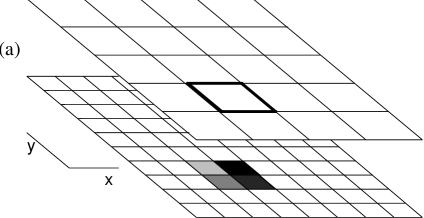
Figure 1: A 2-dimensional representation of the blocking scheme. (a) Each block in the upper panel is constructed by averaging the four cells or blocks beneath it. (b) This picture shows two sets of overlapping grids each of which aligns with the same sub-grid from the previous level of smoothing.

The density fluctuations within blocks and base-cells are now ordered in decreasing density, which is the same order in which they would collapse as the universe ages (under the naïve assumption that they all have the same morphology at all times: we will test the accuracy of this assumption later).

The final step is to build up a merger tree to express the collapse history of blocks. This is a much harder problem than in the simple Block Model because the blocks we use are not always nested inside one another but may overlap. Our initial guess was to merge together all collapsed blocks which overlap with one another, but this leads to very elongated structures which can stretch across a large fraction of the box. While these may represent large-scale pancakes or filaments, they are clearly not the kind of simple virialized halos which we are trying to identify. In practice they would probably break up into smaller objects and so we need to find some way to limit their growth. The procedure we use to do this is as follows:

• First some terminology. Collapsed regions are known as halos. Initially these coincide with the cubical blocks but they need not do so at later times once overlapping blocks begin to collapse. The merger tree consists of a list of cells and sub-halos which constitute each halo. (For simplicity each cell, block or halo also contains a link to its ‘parent’ halo but these are not strictly required).

• Initially, there are no collapsed halos. We start at the top of the ordered list of cells and blocks and run down it in order of increasing collapse time.

• Each cell that collapses is given a parent halo, provided that it has not already been incorporated into some larger structure (this avoids the cloud-in-cloud problem).

• For each block that collapses we first obtain a list of all the halos with which it overlaps and to what extent. The action to be taken depends upon this degree of overlap:

  1. Any uncollapsed cells are added to the new halo. This represents accretion of intergalactic material.

  2. If halos are discovered whose mass is less than that of the block and at least half of which is contained within the block, then these are merged as part of the new structure. This would represent accretion of existing collapsed objects.

  3. If the collapsing block has half or more of its mass contained in exactly one pre-existing halo then merge them together as part of the new structure. This would represent accretion of the block by a larger collapsed object. The restriction to exactly one pre-existing halo prevents the linking together of adjacent halos without the collapse of any new matter (see Fig. 2a). It is this condition which prevents the growth of long filamentary structures and limits the axial ratio of halos to be approximately less than 3:2.

Initially the method produces halos of mass 1 and 8 cell units, but as blocks begin to merge so they produce halos of a wide variety of shapes and a continuous spectrum of masses. The two most common methods of sudden change in halo mass are creation by the merger of several sub-units (Fig. 2b) or accretion of a new block of approximately equal mass which overlaps with the halo (Fig. 2c). These produce approximately cubic structures, or triaxial with axial ratios ranging from 3:2 to 1:1 (Fig. 8). Contrast this with the Block Model where the halo masses always increase by a factor of two at each merger event.

Figure 2: (a) We wish to avoid mergers such as that shown in this diagram where two pre-existing halos (solid boxes) are linked together by the collapse of a third block. This is the reason for the restriction on merging discussed in the text. (b) A typical example of the formation of a new halo by merger of many smaller sub-units. (c) The growth of a halo by accretion of another block of almost equal size.

3 Results

3.1 Self-similarity

We have tested our algorithm on power-law density fluctuation spectra, which should give self-similar scaling on scales much smaller than the box-size. We take a power-law spectrum $P(k)\propto k^{n}$, where $n=-2$ or 0 to span the range of solutions expected in the real Universe. In an infinite box these would translate to a root-mean-square density fluctuation spectrum $\sigma(m)\propto m^{-\alpha}$ where $\alpha=(3+n)/6$. However, in practice we are missing a lot of power outside the box and so the decline is steeper than this at high masses, especially for $n=-2$. This is illustrated in Fig. 3a where the spectrum is clearly not a power-law, but is well-fit by the solid line which shows $\sigma(m)$ calculated by direct summation of waves inside the box with a window function associated with a cubical filter. For $n=0$ the effect is not so severe, so we fit the data with the functional form of $\sigma(m)$ for an infinite box. Note that, because we are using a cubical filter, the normalization is different than it would be for a spherical top-hat. This difference is irrelevant for the purposes of this paper because the normalization we use is arbitrary, however it could be important if we were to compare our predictions with the results of N-body simulations.

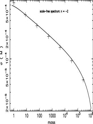
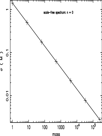
Figure 3: The measured root-mean-square power on various mass-scales for the $128^{3}$ box: (a) $n=-2$, (b) $n=0$. For $n=-2$ the solid line is calculated by direct summation of waves inside the box with a cubical window function. The corresponding curve is normalised to the second point of the data. The plots are in logarithmic scale.

The results presented here were mostly obtained using boxes of side $L=128$. We tried a range of box-sizes, from $L=32$ to 256, to test the effect of variable resolution on our results. The code needs about $2L^{3}$ words of memory so $L=256$ is the largest practical size on a workstation. If the merger tree is to be used as the basis of galaxy formation models, however, then much more storage is required and $L=128$ would be the largest simulation we can allow for.

Fig. 4 shows the cumulative mass function, $F(M,z)$, for $L=128$, averaged over four realizations. The output is shown for four redshifts corresponding to fractions ${1\over 16}$, ${1\over 8}$, ${1\over 4}$ and ${1\over 2}$ of the box contained in collapsed regions for $n=-2$ and fractions ${3\over 16}$, ${1\over 4}$, ${3\over 8}$ and ${1\over 2}$ for $n=0$ (these choices were made simply to get well-spaced curves in the figure: we can reconstruct the curves at any intermediate time). The dashed lines show the corrected Press-Schechter prediction where $\sigma(m)$ is obtained from fits to the points shown in Fig. 3.

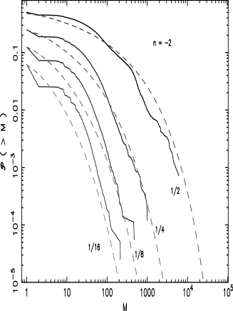
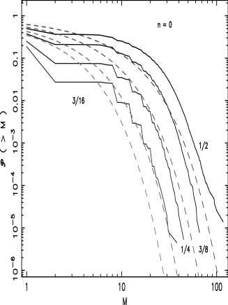
Figure 4: The average cumulative mass function for the four $L=128$ boxes at four different output times (when a certain fraction of the box is in collapsed regions, as indicated by the figures next to the curves) for (a) $n=-2$ and (b) $n=0$. The dashed lines show the corresponding Press-Schechter predictions (with extra factor of two).

In both cases the evolution is approximately self-similar. This can be seen more clearly in Fig. 5 which shows a differential plot, $-\partial F/\partial\ln\nu$, where $\nu=\delta_{c}/\sigma(M,z)$ is the ordinate ($\nu=(M/M_{*})^{1/2}$ for $n=0$). Also shown is the corrected PS prediction,

$$-{\partial F\over\partial\ln\nu}={2\nu\over\sqrt{2\pi}}e^{-{1\over 2}\nu^{2}}.$$ (3)

When expressed in this way the functional form of the mass distribution is absolutely universal, i.e. it does not depend on any parameter of the simulation.

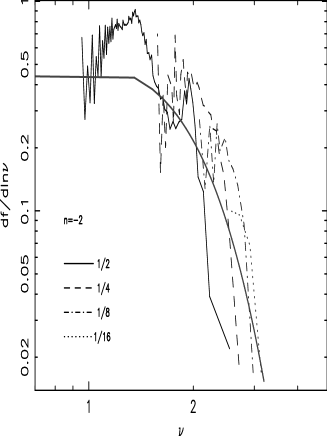
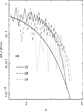
Figure 5: The differential mass function, $\partial f/\partial\ln\nu$, for the $L=128$ box at the times corresponding to the indicated fractions of the box contained in collapsed regions: (a) $n=-2$, (b) $n=0$. The thick dashed line shows the corresponding Press-Schechter prediction.

Consider first the $n=0$ case. Here the differential mass curves seem to have the same shape as the PS prediction, but with a higher normalization (alternatively one could say that $\delta_{c}$ should be reduced slightly so as to shift the predicted curve to the right). This is not unexpected and is discussed in Section 3.3 below. There is no evidence of a departure from the PS curve at a mass of 64, corresponding to the size of smoothing blocks of side 4 (this is in contrast to the $n=-2$ case, discussed below). The maximum mass of collapsed halos is quite small, less than 125 even for the largest box, $L=256$. Given that the smallest halos to collapse in our model (apart from isolated cells) have mass 8, then this gives a very small dynamic range. We could force larger objects to form by allowing a larger fraction of the box to collapse (this would be legitimate if, for example, one were to regard the whole box as a single collapsed halo) however one would not then expect the evolution to be self-similar.

The curves for the steeper spectrum, $n=-2$, extend to much higher masses because the spectrum has much more power on large scales than for $n=0$. Here we do see evidence of kinks at the blocking masses of 64, 512 and 4096, especially at the final output time when half the box has collapsed: there is an excess of halos of slightly higher mass and a deficit of slightly lower mass than these. Overall the spectrum is a reasonable fit to the PS prediction at masses above 100, but shows and excess between masses of 8 and 100.

3.2 Properties of halos

Fig. 6 shows a projection of the largest halos in one $L=128$ box of each spectral type at a time when half the mass has collapsed into halos. Many of the irregular shapes which are visible are due to projection effects.

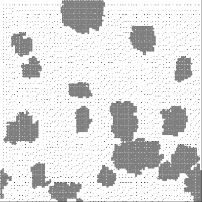
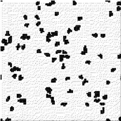
Figure 6: Projections of the distribution of halos taken at the time when half the box is contained in collapsed structures: (a) $n=-2$, mass greater than 700; (b) $n=0$, mass greater than 50.

Our halos tend to exhibit more variety of axial ratios than in the Block Model. There the relative length of the major- and minor-axes is fixed all times at approximately 1:1.59, whereas ours start with more typically 1:1 (for collapse of isolated blocks as in Fig. 2b) or 1:1.5 (for the collapse of overlapping blocks as in Fig. 2c), developping rapidly to more complex structures with a great variety of shapes.

Fig. 8 shows the distribution of axial ratios for all halos of mass greater than or equal to 8 for $n=0$ and greater than 50 for $n=-2$. The overall observation is that there is no much difference of halo shapes if one compare realizations of both spectra. In both, the halos show a wide range of triaxality ranging from prolate to oblate (while in the Block Model they are systematically prolate).

A drawback of our method comes from the fact that the overdensity of a collapsing block, $\delta_{\rm b}$, is not necessarily equal to the mean overdensity of the resulting halo, $\delta_{\rm h}$. It is the former value which we must associate with the halo if the topology of the merger tree is to be preserved (or at least we must maintain the same ordering of densities for halos as their parent blocks). The differences can be quantified in terms of the ratio $\chi=(\delta_{\rm b}-\delta_{\rm h})/\delta_{\rm b}$ which is plotted in Fig. 7 at a time when half the mass is in collapsed structures: we show the mean value plus one sigma error bars.

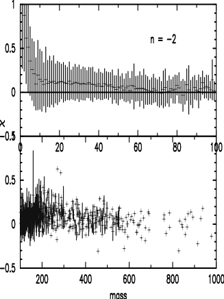
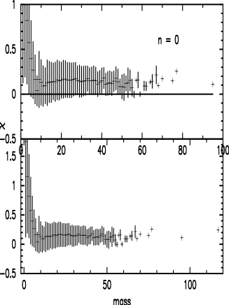
Figure 7: The relative difference between the assigned and the true overdensity of halos, for the $L=128$ box at the time when half of its mass is contained in collapsed regions.

Note first that halos of fewer than eight cells have overdensities which are much less than the assigned one. These structures are, however, leftovers of the merging process (the smallest blocks have a mass of 8 units) and so they should not be considered as collapsed halos, but rather clouds of intergalactic material to be accreted later by a neighbouring halo.

For halos of mass 8 or larger the agreement is much better, but nevertheless the true overdensity of a halo remains systematically lower than the assigned one. The effect is largest for $n=0$ where the mean value of $\chi$ is about 0.15. For $n=-2$, it varies from approximately zero in the largest halos to 0.1 in the low mass ones. The reason for the offset is that high-density cells can contribute to the overdensity of more than one block. Refering again to Fig. 2c, if the region of overlap between the two blocks were of higher density than its surroundings then the density of the whole halo would be lower than that of either block from which it is constructed. If desired the assigned halo densities could be systematically reduced to bring them into agreement with the measured ones; equivalently one could raise the value of the critical density, $\delta_{c}$, required for collapse above that of the top-hat model.

More serious is variance of $\chi$, approximately 0.2, which means that two halos with the same assigned density can have quite disparate true overdensities. The model supposes that they collapse at the same time, whereas the full non-linear evolution would presumably show otherwise. We occasionally find some high-mass halos (mass greater than 8) with big $\chi$, which contribute significantly to the enlargement of the error bars at those scales. These are effectively leftovers of the merging process and should not be treated as collapsed halos in subsequent applications of the method (that is, in a realistic galaxy formation modelling they should be considered as sources of material to be accreted at a later stage of the hierarchy).

The variance in $\chi$ is unwelcome but is only one contribution to the dispersion between overdensity and collapse time. We note that N-body simulations show for each particle a poor correspondence between the expected mass of its parent halo (predicted from the initial conditions) and the true value measured from a numerical simulation, evolved from the same initial conditions (White 1995, Bond et al.  1992). Moreover gravitational collapse is clearly not as simple as the spherical model assumes. There is, for example, no guarantee that underdense regions never collapse or that high-dense regions will do so (Bertschinger & Jain 1994). However, if a simple semi-analytical model of the gravitational clustering is desired, then the simple relation between collapse redshift and initial overdensity given by the spherical model seems the most obvious choice.

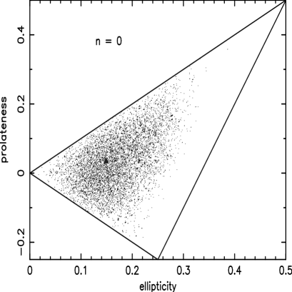
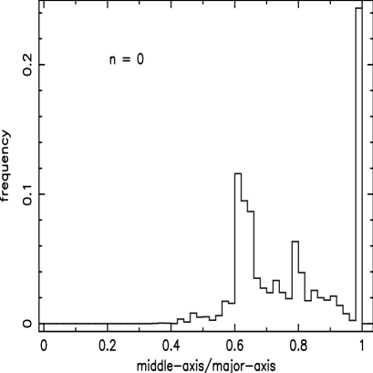
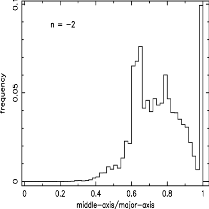
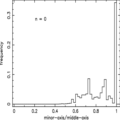
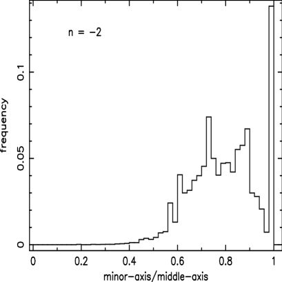
Figure 8: Distribution of axial ratios for halos taken from one $L=128$ realization when half of the box mass is contained in collapsed structures: $n=0$, mass greater or equal than 8; $n=-2$, mass greater than 50. The upper panel shows the distribution of triaxalities in the prolateness-ellipticity plane (with the filled triangle corresponding to the Block Model).

3.3 The number density of high-mass halos

Our method passes the test for self-similarity, yet for $n=0$ it predicts far more high-mass halos than Press-Schechter or other methods based on similar ideas, such as the Block Model. This is an expected outcome of our method and points more to a deficiency in the PS model than anything else, as we attempt to explain below.

Press-Schechter does not count the number of halos of a given mass. Rather, it counts the fraction of the Universe where, if one were to put down a top-hat filter of the appropriate mass, the overdensity would exceed a certain critical threshold. Regions which just poke above this threshold for a single position of their centres, contribute nothing to the mass-function. It is easy to see that this becomes increasingly likely as one moves to rarer and rarer objects (of higher and higher mass). For these it is much better simply to count the number of peaks which exceed the threshold density after filtering on the appropriate scale (on the other hand Peaks Theory predicts far too many low-mass objects as it does not distinguish between overlapping halos). The necessary theory has been exhaustively analyzed by Bardeen et al. (1986) who showed that uncorrected PS (without the extra factor of two) underestimates the number of high-mass halos by a factor $\alpha^{3/2}\nu^{3}$, where $\delta_{c}=\nu\sigma(m)$ (this result is for a gaussian filter but similar results will hold for all filters with just a small difference in scaling). One way to visualize this result is to think of each peak as having an overdensity profile

$$\nu\approx\nu_{0}\left(1-{1\over 2}\left(r\over R\right)^{2}\right)$$ (4)

where $R$ is the radius of the top-hat filter. It is then easy to estimate the contribution to the PS mass fraction and to integrate over all values of $\nu_{0}$ greater than the threshold, $\delta_{c}/\sigma$, to get the total number of halos. This method suggests that PS should predict $\sqrt{2/9\pi}\,\nu^{3}$ times as many halos as Peaks Theory, in rough agreement with the above for $n\approx-1$ to 0.

A more direct demonstration of the above difference between Press-Schechter and the actual number of high-mass peaks in the density field is shown by the numbers in Table 1. Columns 2–9 show the measured number of blocks which exceed the density threshold given in the first column in each of the eight sub-grids of mass 512.

Table 1: Number of blocks of mass 512 ($L=128$) above the density thresholds $3\sigma$, $2\sigma$, $\sigma$: (a) $n=-2$, (b) $n=0$. Columns 2–9 correspond to each of the eight sub-grids used for that level of refinement, Column 10 shows the number of isolated peaks and Column 11 the PS prediction of the expected number of halos of this mass.

(a) XYZ	single								combined	PS expected
grid	grid	X	Y	Z	XY	XZ	YZ	XYZ	grids	number
$\geq 3\sigma$	5	7	4	1	6	7	6	8	18	5.5$\pm$2.3
$\geq 2\sigma$	88	87	92	77	92	87	79	88	109	93.2$\pm$9.7
$\geq 1\sigma$	628	654	630	662	628	648	639	647	281	650$\pm$26

(b) XYZ	single								combined	PS expected
grid	grid	X	Y	Z	XY	XZ	YZ	XYZ	grids	number
$\geq 3\sigma$	6	7	4	9	4	7	8	7	38	5.5$\pm$2.3
$\geq 2\sigma$	99	99	96	82	90	86	99	90	324	93.2$\pm$9.7
$\geq 1\sigma$	630	641	649	656	652	617	670	677	671	650$\pm$26

These agree with the Press-Schechter prediction, as indeed they should by construction. When we combine the various grids, however, an interesting thing happens. Column 10 shows the number of separate, (i.e. non-overlapping), overdense blocks in the combined grid. At high overdensity all the halos we have identified are distinct (they exceed the threshold for just one position of the smoothing grid). The total number of halos is therefore greatly in excess of the PS prediction and far closer to that given by Peaks Theory. For $n=-2$ the excess is approximately a factor of three which brings them into agreement once the PS prediction has the extra factor of two applied. For $n=0$, however, the difference is much larger and the number of peaks is a factor of 3-4 larger than even the corrected PS estimate. This goes in some way to explaining the difference between the PS prediction and the measured cumulative mass function in Fig. 4.

At lower overdensity the disagreement is much less severe. One should note that for $n=-2$ there is a gross underestimate of $1\sigma$ peaks compared to the values obtained in each sub-grid. This is simply a consequence of the Peaks methodology. Remember that for each sub-grid we are just measuring the fraction of the total number of blocks above the threshold, while in the case of combined grids we simply count the number of peaks. Because for $n=-2$ the peaks are larger and more clustered, there is a great chance of finding blocks sitting next each other which are above the imposed threshold. Consequently, if we are only selecting the peaks many of those blocks will be discarded. This situation does not arise for $n=0$, where the peaks are smaller and more evenly distributed.

Our use of overlapping grids is therefore crucial. They ensure that all halos are approximately centred within one of the grid cells. Other methods, such as the Block Model, which have fixed borders between mass cells, have difficulty in detecting structures that cross cell boundaries and are, by construction, forced to agree with Press-Schechter. This can lead to a gross underestimate of the number of rare, high-mass peaks, especially for steep spectra. We are not saying that our method necessarily gives a better description of the growth of structure in the Universe because all these theoretical models are highly idealized. Substructure may lengthen collapse times and tidal field may need to be taken into account. Nevertheless, given the simplified prescription which we have adopted, our method does at least seem to detect the correct number of high-mass halos, and many more than other methods.

4 Discussion

We have presented a new method of constructing a hierarchical merger tree based on actual realizations of the linear density field. We smooth on a set of interlaced, cubical grids on a variety of mass scales, then order in decreasing density. We run down the resulting list, merging together overlapping blocks to form collapsed halos. The main properties of our model are as follows:

• The model exhibits the scaling behaviour expected from power-law spectra.

• For a flat, white-noise spectrum, $n=0$, the mass function is well-fit by the PS model, provided that we raise the normalization by a factor of 3-4. This difference arises because of a deficiency in the PS method which fails to count the correct number of massive, rare (high-$\nu$) peaks. The dynamic range for the masses of halos for this spectrum is quite small—at a time when half the box is in collapsed structures, the mass of the largest halo is just 125 cells, even for the box of side $L=256$.

• The mass function for a steeper spectrum, $n=-2$, lie much closer to the PS prediction (with the usual factor of two increase in normalization), but show small kinks at masses of 64, 512 and 4096, corresponding the the masses of smoothing blocks—there is a slight deficit of halos of smaller, and an excess of halos at larger, mass.

• The collapsed halos tend to be triaxial with a wide mixture of prolateness and oblateness (contrary to the Block Model).

• The mean overdensity of halos tends to be lower than that assigned to them by our scheme, and to have a scatter of about 20 percent about the mean value. While undesirable, since it can reverse the collapse ordering in the tree, this can be partialy cured in subsequent applications of the method.

A shortcoming of our method is that the minimum halo mass is eight cells with a corresponding loss of dynamical range. We see in Fig. 4 that for $n=-2$ we achieve approximately a mass-range of approximately two and a half decades when half the mass is contained in collapsed objects, while for $n=0$ we get only slightly more than one decade. This is because $n=-2$ corresponds to a flat spectrum, $\sigma\propto M^{-1/6}$, with almost all scales collapsing simultaneously, while for $n=0$ the spectrum decreases more rapidly, $\sigma\propto M^{-1/2}$, and the peaks are much more isolated. Fortunately, the physically-motivated CDM spectrum can be fitted by an $n=-2$ spectrum over a significant mass range, and so the loss of dynamical range is not so important in a realistic application of the method. All these mass-ranges can be extended if we allow a larger fraction of the box to collapse (as we must if we wish to model a cluster of galaxies, for example), but at the risk of losing a fair representation of the power spectrum on scales approaching the box-size.

If we simulate a large portion of the Universe, of mass say $10^{16}\hbox{$\rm\thinspace M_{\odot}$}$, in a box of $L=128$, then a block of 8 cells corresponds to $3.8\times 10^{10}$$\rm\thinspace M_{\odot}$, which could represent at best a dwarf galactic halo. If the box represents a large galactic halo of mass $10^{13}\hbox{$\rm\thinspace M_{\odot}$}$, then we can resolve down almost to globular cluster scales.

We also have carried out simulations with a range of box-lengths, $L=16$, 32, 64, 128, and 256, in order to show the effect of variable resolution (we were not able to perform the $L=16,32$ simulations for $n=0$ due to the lack of dynamical range). The base-cells in each case correspond to one set of blocks of side $256/L$ in the $L=256$ simulation. The results are presented in Fig. 9 which shows the cumulative mass functions sampled at the same collapsed fractions of the box as those corresponding to Fig. 4. The shape of the mass spectrum is similar but with a slight increase in dynamic range as one moves from $L=64$ to $L=256$.

Figure 9: The cumulative mass-function for boxes of variable resolution, as indicated: (a) $n=-2$, (b) $n=0$. The collapsed fractions are the same as those corresponding to Fig. 4 respectively.

Whether our method provides a better description of the formation of structure than other methods remains to be seen. The Block Model in particular seems to give good agreement with N-body simulations (Lacey & Cole 1994) which themselves are approximately fit by modified Press-Schechter models (e.g. Gelb & Bertschinger 1994). However, there is a limited dynamical range in the simulations, the results are sensitive to the precise model for identifying collapsed halos and the critical overdensity for collapse is usually taken as a free parameter. Given these caveats it is hard to tell whether the fits are mediocre, adequate or good.

One advantage of our scheme is that it is based on an actual realization of a density field which can be used as the starting point for an N-body simulation. Thus we will not be limited to a statistical analysis, but will be able to directly compare individual structures identified in the linear density field with non-linear halos that form in the simulation. Initial results from other studies (Bond et al. 1992, Thomas & Couchman 1992 ) suggest that the correspondence is approximate at best, and we may be forced to consider the effect of tidal fields on a halos evolution. We have not yet carried out the necessary N-body simulations because we have not up to now had access to the necessary super-computing facilities to evolve (and analyze!) a $256^{3}$ box of particles. Such datasets will soon become available as part of the Virgo Consortium project on the UK’s Cray T3D facility and we intend to report the results in a subsequent paper.

Nevertheless, even in the absence of the numerical tests, we feel that our method is a viable alternative to other methods of calculating the merging history of galactic halos. It passes the test of self-similarity yet predicts more high-mass halos than other methods. It has the disadvantage of losing a factor of eight in resolution at low-masses, but above this it has a smooth mass-spectrum and is not restricted to masses which are a power of two. We intend to contrast the predictions of the Block Model and this current method in models of galaxy formation such as those discussed by Kauffmann, White & Guiderdoni (1993) and Cole et al. (1994), and explore the role of pre-galactic cooling flows (Nulsen & Fabian 1995).

References

- [] Bardeen J.M., Bond J.R., Kaiser N., Szalay A.S., 1986, ApJ, 304, 15
- [] Bertschinger E., Jain B., 1994, ApJ, 431, 486
- [] Bond J.R., Cole S., Efstathiou G., Kaiser N., 1992, ApJ, 379, 440
- [] Bower R.J., 1991, MNRAS, 248,332
- [] Cole S., Kaiser N., 1989, MNRAS, 237, 1127
- [] Cole S., 1991, ApJ, 367, 45
- [] Cole S., Aragon-Salamanca A., Frenk C.S., Navarro J.F., Zepf S.E., 1994, MNRAS, 271, 781
- [] Efstathiou G., Frenk C.S., White S.D.M., Davis M., 1988, MNRAS, 235, 715
- [] Gunn J.E., Gott J.R., 1972, ApJ, 176, 1
- [] Gelb J.M., Bertschinger E., 1994, ApJ, 436, 467
- [] Kauffmann G., White S.D.M., 1993, MNRAS, 261, 921
- [] Kauffmann G., White S.D.M., Guiderdoni B., 1993, MNRAS, 264, 201
- [] Lacey C.G., Cole S., 1993, MNRAS, 262, 627
- [] Lacey C.G., Cole S., 1994, MNRAS, 271, 676
- [] Nulsen P.E.J., Fabian A.C., 1995, MNRAS, Preprint astro-ph/9506014
- [] Press W.H., Schechter P.G., 1974, ApJ, 187, 425
- [] Thomas P.A., Couchman H.M.P., 1992, MNRAS, 257, 11
- [] White S.D.M., 1995, Formation and Evolution of Galaxies: Lectures given at Les Houches, August 1993