The cluster abundance in flat and open cosmologies

Abstract

We use the galaxy cluster X-ray temperature distribution function to constrain the amplitude of the power spectrum of density inhomogeneities on the scale corresponding to clusters. We carry out the analysis for critical-density universes, for low-density universes with a cosmological constant included to restore spatial flatness and for genuinely open universes. That clusters with the same present temperature but different formation times have different virial masses is included. We model cluster mergers using two completely different approaches, and show that the final results from each are extremely similar. We give careful consideration to the uncertainties involved, carrying out a Monte Carlo analysis to determine the cumulative errors. For critical density our result agrees with previous papers, but we believe that the result carries a larger uncertainty. For low-density universes, either flat or open, the required amplitude of the power spectrum increases as the density is decreased. If all the dark matter is taken to be cold, then the cluster abundance constraint remains compatible with both galaxy correlation data and the COBE measurement of microwave background anisotropies for any reasonable density.

1 Introduction

One of the most important constraints that a model of large-scale structure must pass is the ability to generate the correct number density of galaxy clusters. This is a crucial constraint, because a considerable amount is known about clusters from both optical and X-ray measurements. As clusters are relatively rare objects, in the standard picture they must form from fairly high peaks in the original density field and hence their abundance is very sensitive to the normalization of the power spectrum on those scales. As a result, the cluster abundance has been cited (White, Efstathiou & Frenk 1993) as one of the strongest pieces of evidence against the standard cold dark matter (CDM) model when that model is normalized so as to reproduce the microwave background anisotropies as seen by the COBE satellite [Bennett et al. 1996, Banday et al. 1996, Górski et al. 1996, Hinshaw et al. 1996].

Amongst the many ways in which the CDM model can be salvaged, a popular choice has been to reduce the total matter density. The most common context within which such models have been studied is in spatially flat cosmologies, where a cosmological constant has been introduced to make up the shortfall in the matter density [Efstathiou, Sutherland & Maddox 1990, Kofman, Gnedin & Bahcall 1993, Klypin, Primack & Holtzman 1995]. However, recently attention has also been focused on the possibility of a genuinely open cosmological model [Ratra & Peebles 1994, Górski et al. 1995, Liddle et al. 1996a], which possesses somewhat different late-time dynamics and also a different COBE normalization.

In this paper, we re-assess the cluster abundance constraint in CDM models, encompassing spatially flat models with both a critical and sub-critical matter density and also open universe models. We use the X-ray temperature distribution function, taking advantage of a number of extensive hydrodynamical cluster simulations which have now been carried out to calibrate this to Press–Schechter theory.

2 The Power Spectrum

Except for a brief discussion on COBE near the end of the paper, we shall be interested in scales short enough that even in the open case one can consider space to be flat. This allows us to specify the power spectrum of the density contrast, following the notation of Liddle & Lyth [Liddle & Lyth 1993] and Liddle et al. [Liddle et al. 1996a], as

$${\cal P}_{\delta}(k)=\left(\frac{k}{aH}\right)^{4}T^{2}(k)\,\delta_{{\rm H}}^{2}(k)\,\frac{g^{2}(\Omega)}{g^{2}(\Omega_{0})}\,,$$ (1)

where $k$ is the wave number, $a$ is the scale factor, $H=\dot{a}/a$ is the Hubble parameter, $\Omega$ is the density parameter, subscript ‘0’ indicates the present value, $T(k)$ is the transfer function and the factor $g(\Omega)$, defined later, accounts for the rate of growth of density perturbations relative to the critical-density case whose growth is given by the $(aH)^{4}$ factor. The quantity $\delta_{{\rm H}}^{2}(k)$ specifies the shape of the primordial spectrum; it is a constant for the Harrison–Zel’dovich spectrum, and $\delta_{{\rm H}}^{2}\propto k^{n-1}$ for a ‘tilted’ spectrum with spectral index $n$. A quantity related to the power spectrum is the dispersion $\sigma(R)$ of the density field smoothed on a (comoving) scale $R$, defined by

$$\sigma^{2}(R)=\int_{0}^{\infty}W^{2}(kR)\,{\cal P}_{\delta}(k)\frac{{{\rm d}}k}{k}\,.$$ (2)

To carry out the smoothing, we shall always use a top-hat window function $W(kR)$ defined by

$$W(kR)=3\left(\frac{\sin(kR)}{(kR)^{3}}-\frac{\cos(kR)}{(kR)^{2}}\right)\,.$$ (3)

A large galaxy cluster has a mass of around $10^{15}\,{\rm M}_{\sun}$; the amount of matter required to make such a cluster would originally (before collapse) be contained in a comoving sphere of radius $9.5(h/\Omega_{0})^{1/3}h^{-1}$ Mpc, where $h$ is the present Hubble constant in units of $100\,{\rm km}\,{\rm s}^{-1}\,{\rm Mpc}^{-1}$. Traditionally, the cluster abundance is used to place a constraint on the dispersion of the density contrast at the scale $8h^{-1}$ Mpc, denoted $\sigma_{8}$, and some assumption regarding the shape of the power spectrum is required to shift from the scale actually constrained by the observations on to this one. For CDM models as considered here, the power spectrum is accurately given by Bardeen et al. [Bardeen et al. 1986] as

$$T_{{\rm CDM}}(q) = \frac{\ln\left(1+2.34q\right)}{2.34q}\times$$

$$\left[1+3.89q+(16.1q)^{2}+(5.46q)^{3}+(6.71q)^{4}\right]^{-1/4}\,,$$

with $q=k/h\Gamma$, where the ‘shape parameter’ $\Gamma$ is defined as [Sugiyama 1995]

$$\Gamma=\Omega_{0}h\exp(-\Omega_{{\rm B}}-\Omega_{{\rm B}}/\Omega_{0})\,,$$ (5)

with $\Omega_{{\rm B}}$ the baryon density. This fit to $\Gamma$ is good for both flat and open universes. However, we have no particular need for it, as we can simply specify models by $\Gamma$. If the spectral index $n$ equals $1$, then, provided that $\Gamma$ is chosen in the range $\Gamma=0.230^{+0.042}_{-0.034}$ (these limits being 95 per cent confidence), a reasonable fit to the shape of the galaxy correlation function is obtained. This allowed interval for $\Gamma$ was calculated using the data points in table 1 of Peacock & Dodds [Peacock & Dodds 1994], omitting the four corresponding to the smallest scales, as at these scales the working assumption of a linear bias used in their calculation seems to break down (Peacock 1996). Because galaxy correlations are presumed to be biased relative to the mass, this fit tells us nothing about the overall normalization of the matter power spectrum.

It is simplest to use an approximation to the true shape of $\sigma(R)$ in the vicinity of $8h^{-1}$ Mpc. White et al. [White et al. 1993a] use a power-law fit where the exponent is related to $\Gamma$. Because, particularly for low densities, we require accuracy over a greater range of scales, we use the more accurate fit

$$\sigma(R)=\sigma_{8}\left(\frac{R}{8h^{-1}\;{\rm Mpc}}\right)^{-\gamma(R)}\,,$$ (6)

where for the CDM spectra we adopt the form

$$\gamma(R)=(0.3\Gamma+0.2)\left[2.92+\log\left(\frac{R}{8h^{-1}\;{\rm Mpc}}\right)\right]\,.$$ (7)

If one chooses a tilted primordial spectrum, $n\neq 1$, then the best-fitting $\Gamma$ is changed, but the actual shape of the power spectrum is still obliged to fit the shape of the galaxy correlation function and so the results that we obtain will not depend significantly on $n$; indeed, even the $\Gamma$ dependence will prove unimportant provided that it is restricted to lie within the favoured range.

In a critical-density universe, clusters are anticipated to have formed very recently. As we shall see, in low-density universes clusters will have formed much earlier, and we shall need to take into account the redshift dependence of the power spectrum. In CDM universes, the shape of the power spectrum is unchanged at low redshift, so we need only consider the redshift dependence at a single scale which we take to be $8h^{-1}$ Mpc. This dependence is different depending on whether we have an open model (which we label ‘OCDM’) or a flat model (which we label ‘$\Lambda$CDM’). Following Carroll, Press & Turner [Carroll et al. 1992] we introduce a growth suppression factor $g(\Omega)$, as used in equation (1). This gives the total suppression of growth of the dispersion relative to that of a critical-density universe, and is accurately parametrized by

$$g(\Omega) = \frac{5}{2}\Omega\left[1+\frac{\Omega}{2}+\Omega^{4/7}\right]^{-1}\quad\quad\quad\quad\quad{\rm(OCDM)}\,;$$ (8)

$$g(\Omega) = \frac{5}{2}\Omega\left[\frac{1}{70}+\frac{209\Omega}{140}-\frac{\Omega^{2}}{140}+\Omega^{4/7}\right]^{-1}\,{\rm(}\Lambda{\rm CDM)}.$$ (9)

These formulae can be applied at any value of $\Omega$. For a matter-dominated low-density universe, the redshift dependence of $\Omega$ is given by

$$\Omega(z) = \Omega_{0}\,\frac{1+z}{1+\Omega_{0}z}\quad\quad\quad\quad\quad\quad\quad{\rm(OCDM)}\,;$$ (10)

$$\Omega(z) = \Omega_{0}\,\frac{(1+z)^{3}}{1-\Omega_{0}+(1+z)^{3}\Omega_{0}}\quad\quad{\rm(}\Lambda{\rm CDM)}\,.$$ (11)

Since the growth law in a critical-density universe is $\sigma_{8}(z)\propto(1+z)^{-1}$, the redshift dependence for arbitrary $\Omega_{0}$ is therefore

$$\sigma_{8}(z)=\sigma_{8}(0)\,\frac{g(\Omega(z))}{g(\Omega_{0})}\,\frac{1}{1+z}\,,$$ (12)

using the appropriate formulae for $g(\Omega)$ and $\Omega(z)$ depending on whether the universe is open or flat.

3 Press–Schechter Theory

3.1 Number densities

The most accurate way of assessing the cluster abundance is via numerical simulation. However, there is an excellent analytic alternative which is the Press–Schechter theory [Press & Schechter 1974, Bond et al. 1991]. For the case of a critical-density universe, this has been extensively tested against $N$-body simulations and found to fare extremely well [Lacey & Cole 1994]. Less attention has been directed towards testing the theory in open universes, but those studies that do exist suggest that it continues to work well, as one might expect since its derivation relies only on statistical arguments.

Press–Schechter theory states that the fraction of material residing in gravitationally bound systems larger than some given mass $M$ is given by the fraction of space in which the linearly evolved density field, smoothed on that mass scale, exceeds some threshold $\delta_{{\rm c}}$. Originally the choice of $\delta_{{\rm c}}$ was motivated via the spherical collapse model, but it should now be calibrated via $N$-body simulations. The appropriate formula is

$$\frac{\Omega(>M(R),z)}{\Omega(z)}={\rm erfc}\left(\frac{\delta_{{\rm c}}}{\sqrt{2}\,\sigma(R,z)}\right)\,,$$ (13)

where ‘erfc’ is the complementary error function. Here $R$ is the comoving linear scale associated with $M$, $R^{3}=3M/4\pi\rho_{{\rm b}}$, where $\rho_{{\rm b}}$ is the comoving background density which is constant during matter domination. In equation (13), the right hand side has been multiplied by a factor two to allow the material in underdense regions to participate; in original treatments this seemed very ad hoc but it has now been more or less well justified [Peacock & Heavens 1990, Bond et al. 1991], and in any case it is incorporated in the $N$-body calibration. The required value of $\delta_{{\rm c}}$ is quite dependent on the choice of smoothing window used to obtain the dispersion [Lacey & Cole 1994]. We shall use a top-hat window function. Were one to use a Gaussian window the threshold would be significantly lower (or alternatively the associated mass could be increased as discussed by Lacey & Cole 1994); claims in the literature of a large uncertainty in the Press–Schechter calculation are often due to quoting thresholds for different types of smoothing and one should always be careful to specify which is being used.

For spherical collapse, the appropriate threshold is $\delta_{{\rm c}}=1.7\pm 0.1$. In the generic non-spherical situation, one must be careful to specify what is meant by collapse; if one considers collapse along all three axes the threshold is higher, whereas collapse along the first axis (pancake formation) or the first two axes (filament formation) corresponds to a lower threshold [Monaco 1995]. Since large clusters are relatively rare, one can assume that shear did not play an important role and hence their collapse can be considered to have occurred spherically [Bernardeau 1994].

One might expect $\delta_{{\rm c}}$ to depend on the background cosmology. However, this seems not to be the case — Lilje [Lilje 1992], Lacey & Cole [Lacey & Cole 1993] and Colafrancesco & Vittorio [Colafrancesco & Vittorio 1994] found that, at least for any type of collapse where $\delta_{{\rm c}}\leq 1.7$ in a flat universe, the value of $\delta_{{\rm c}}$ varies at most by $5$ per cent when one goes from a critical-density universe to one with $\Omega_{0}=0.1$. Since at earlier epochs low-density universes become closer to critical-density ones, the variation will be even less as one goes to higher redshifts.

Equation (13) gives the total amount of material in structures above a given mass. However, we shall be interested in the number density of objects within a given mass range. The comoving number density of clusters in a mass interval ${\rm d}M$ about $M$ at a redshift $z$ is obtained by differentiating equation (13) with respect to the mass and multiplying it by $\rho_{{\rm b}}/M$. This gives

$$n(M,z)\,{\rm d}M=$$

$$-\sqrt{\frac{2}{\pi}}\frac{\rho_{{\rm b}}}{M}\,\frac{\delta_{{\rm c}}}{\sigma^{2}(R,z)}\frac{{\rm d}\sigma(R,z)}{{\rm d}M}\exp\left[-\frac{\delta_{{\rm c}}^{2}}{2\sigma^{2}(R,z)}\right]{\rm d}M\,.$$

Following White et al. [White et al. 1993a], we can simplify this for $R$ in the vicinity of $8h^{-1}$ Mpc by using our analytic approximation to the power spectrum, equation (6), to calculate the derivative in equation (3.1). This gives

$$n(M,z)\,{\rm d}M=$$

$$\sqrt{\frac{2}{\pi}}\frac{\rho_{{\rm b}}}{M^{2}}\frac{2.92(0.3\Gamma+0.2)\delta_{{\rm c}}}{3\sigma(R,z)}\exp\left[-\frac{\delta_{{\rm c}}^{2}}{2\sigma^{2}(R,z)}\right]{\rm d}M.$$

3.2 Formation redshifts

We shall be interested in the formation redshifts of the clusters that we see at the present epoch. The literature contains two very different ways of obtaining this (Lacey & Cole 1993, 1994; Sasaki 1994), which each have their advantages and disadvantages. In this paper we shall consider both.

Sasaki [Sasaki 1994] showed through simple physical and mathematical arguments that the comoving number density of clusters with mass in a range ${\rm d}M$ about $M$, which virialize in an interval ${\rm d}z$ about some redshift $z$ and survive until the present without merging with other systems, is given by

$$N(M,z)\,{\rm d}M\,{\rm d}z=$$

$$\left[-\frac{\delta_{{\rm c}}^{2}}{\sigma^{2}(R,z)}\frac{n(M,z)}{\sigma(R,z)}\frac{{\rm d}\sigma(R,z)}{{\rm d}z}\right]\frac{\sigma(R,z)}{\sigma(R,0)}\,{\rm d}M\,{\rm d}z\,.$$

The redshift independence of the shape of the CDM power spectrum allows us to write

$$N(M,z)\,{\rm d}M\,{\rm d}z=$$

$$\left[-\frac{\delta_{{\rm c}}^{2}}{\sigma^{2}(R,z)}\frac{n(M,z)}{\sigma_{8}(z)}\frac{{\rm d}\sigma_{8}(z)}{{\rm d}z}\right]\frac{\sigma_{8}(z)}{\sigma_{8}(0)}\,{\rm d}M\,{\rm d}z\,,$$

where $\sigma_{8}(z)$ and ${\rm d}\sigma_{8}(z)/{\rm d}z$ are calculated using equation (12). In equation (3.2), the expression within the square brackets gives the formation rate of clusters with mass $M$ at redshift $z$, whereas the factor outside gives the probability of these clusters surviving until the present. The approximation leading to this equation was to assume that the efficiency of the destruction rate of clusters through mergers has no characteristic mass scale, so that merging proceeds in a self-similar way along the entire mass range. Though we do not expect this to happen for physically motivated power spectra, such as the ones under consideration, it should be a fairly good approximation across a limited range of scales. In order to be consistent with the Press–Schechter formalism, it then turns out that the efficiency of the destruction rate must be only a function of redshift. Blain & Longair (1993a,b) also worked within the Press–Schechter framework, instead assuming various physically reasonable merger probability distributions, and they found results numerically similar to Sasaki’s.

An alternative approach is that of Lacey & Cole (1993, 1994), who attempted to construct a merging history for dark matter haloes based on the random walk trajectories technique. This approach is much closer to physical reality than that of Sasaki, but necessarily much more complicated. They considered two alternative possible techniques for computing the distribution of halo formation times, one based on an analytical counting method and the other based on Monte Carlo generated merging histories; a comparison they made with results from $N$-body simulations shows clearly that the first method is better, providing a good fit to the $N$-body results. In general, the calculation of the distribution of halo formation times using the analytical counting method has to be performed numerically, but for a white noise power spectrum, $n=0$, an analytic expression is available. Usefully, it turns out that the distribution of halo formation times is almost independent of the shape of the power spectrum, so one can use the analytical expression for $n=0$ as a good approximation to the numerical calculation for any $n$.

A drawback of the Lacey & Cole approach is that one has to choose when to consider a given dark matter halo to have formed, since the last infinitesimal amount of mass is still being accreted at the present. That is, at what fraction of its final mass is a halo to be considered to have effectively formed? Bearing in mind that different properties of a cluster may be affected to different degrees by increasing the cluster mass, clearly the definition of when a cluster has effectively formed depends on the particular cluster property under study. A cluster will have effectively formed if the property barely changes until the cluster reaches its final mass. According to Lacey & Cole (1993, 1994), the probability that a cluster with present virial mass $M$ would have formed at some redshift $z$ is then given by

$$p(z)=p(w(z))\frac{{\rm d}w(z)}{{\rm d}z}\,,$$ (18)

where

$$p(w(z))=2\,w(z)\left(f^{-1}-1\right)\,{\rm erfc}\left(\frac{w(z)}{\sqrt{2}}\right)-$$

$$\sqrt{\frac{2}{\pi}}\left(f^{-1}-2\right)\exp{\left(-\frac{w^{2}(z)}{2}\right)}\,,$$

and

$$w(z)=\frac{\delta_{{\rm c}}\left(\sigma(M,0)/\sigma(M,z)-1\right)}{\sqrt{\sigma^{2}(fM,0)-\sigma^{2}(M,0)}}\,,$$ (20)

with $f$ the fraction of the cluster mass assembled by redshift $z$. As the shape of the CDM power spectrum is redshift independent we have $\sigma(M,0)/\sigma(M,z)=\sigma_{8}(0)/\sigma_{8}(z)$, where $\sigma_{8}(z)$ is given by equation (12). Expression (3.2) was obtained for a power-law spectrum with index $n=0$, but, as mentioned before, numerical results show that $p(w(z))$ depends only very weakly on $n$ (Lacey & Cole 1993) so we will use it even though, at the scales we are interested in, the spectral index is closer to $n=-2$.

4 The Cluster Abundance

The first attempts to constrain the power spectrum via the cluster abundance were made by Evrard [Evrard 1989] and then by Henry & Arnaud [Henry & Arnaud 1991]. They both considered only the critical-density case, Evrard using the velocity dispersion to determine the mass via the virial theorem while Henry & Arnaud used the X-ray temperature. Both obtained very similar results, though the quoted errors of the latter were much smaller. Other pre-COBE analyses were made by Bond & Myers [Bond & Myers 1992], by Bahcall & Cen (1992, 1993), by Lilje [Lilje 1992] who considered low-density flat models and by Oukbir & Blanchard [Oukbir & Blanchard 1992] who discussed the open case. Subsequent to the COBE observations, White et al. [White et al. 1993a] carried out an analysis with extra input from $N$-body simulations, obtaining a similar result again to Evrard [Evrard 1989] and Henry & Arnaud [Henry & Arnaud 1991] in the case of critical density and extending the calculation to the case of flat universes with a low matter density. Bartlett & Silk [Bartlett & Silk 1993] tested a variety of flat-space models against the data, using the then current first year COBE normalization which is some way below that currently recommended [Górski et al. 1996]. Balland & Blanchard [Balland & Blanchard 1995] considered the hot dark matter case. Recently, Liddle et al. [Liddle et al. 1996a] briefly described a new calculation in the case of an open universe. That calculation extended the type of analysis made earlier, by attempting to take into account that clusters with equal mass which virialize at different redshifts have distinct properties, such as velocity dispersion and X-ray temperature, at the present. As well as providing a more detailed account of that open universe calculation, in this paper we carry out a similar analysis for flat universes.

When applied to rare objects, the number density predicted by the Press–Schechter theory is extremely sensitive to the dispersion $\sigma(R)$. This is of great advantage, because it means that even if the number density is not well known the error this induces in estimating $\sigma_{8}$ is small. Much more crucial in this application is to establish estimates of the cluster masses as accurately as possible. There are presently three methods in use for mass estimation. The cluster velocity dispersion provides one such means. Unfortunately, cluster catalogues assembled from optical data are prone to contamination from foreground and background galaxies mis-identified as part of the cluster, and may also be affected by projection effects and by the possibility of velocity bias. An alternative means of cluster identification is via X-ray emission from the gas resting in a deep potential well. Since X-rays are produced only in clusters, there are no problems with foreground and background contamination (unless two clusters happen to lie on top of one another in projection, and even then discrimination may be possible as luminosity goes as a steep power of the cluster richness [Henry & Arnaud 1991]). The final method is via weak lensing of background galaxies [Kaiser & Squires 1993]. This promises to be a very interesting technique for the future, but at present has not been widely applied. Consequently, we choose to adopt the X-ray data.

The observed number density of clusters per unit temperature, $n(k_{{\rm B}}T)$, at $z=0$ has been determined by Edge et al. [Edge et al. 1990] and by Henry & Arnaud [Henry & Arnaud 1991]. These are in good agreement; we shall use the latter. We shall concentrate on large clusters by considering those with mean X-ray temperature 7 keV; those are observed to have a present number density per unit temperature interval of

$$n(7\;{\rm keV},0)=2.0_{-1.0}^{+2.0}\times 10^{-7}h^{3}\;{\rm Mpc}^{-3}\;{\rm keV}^{-1}\,.$$ (21)

In order to apply the Press–Schechter formalism, one needs to relate the X-ray temperature to the virial mass. As we shall see, in the case of a critical-density universe one expects that all clusters formed fairly recently and there is more or less a one-to-one correspondence between a given temperature and a given virial mass. In low-density universes, clusters can form much earlier, and the clusters we see today of a given temperature would have formed at a range of different redshifts. Lilje [Lilje 1992] (see also Hanami 1993) has demonstrated that clusters of the same present temperature, but different formation times, will in general have different virial masses in accordance with the scaling relation

$$M_{{\rm v}}\propto\Omega_{0}^{-1/2}\,\chi^{-1/2}\,\left(2\frac{r_{{\rm v}}}{r_{{\rm m}}}\right)^{3/2}\times$$

$$\left[1-\eta\left(\frac{r_{{\rm v}}}{r_{{\rm m}}}\right)^{3}\right]^{-3/2}\,(1+z_{{\rm c}})^{-3/2}\,(k_{{\rm B}}T)^{3/2}h^{-1}\,,$$

where

$$\chi=\left(\frac{4}{3\pi}\right)^{2}\xi\,,$$ (23)

$$\eta=2\left(\frac{4}{3\pi}\right)^{2}\left(\frac{\lambda_{0}}{\Omega_{0}}\right)\chi^{-1}(1+z_{{\rm m}})^{-3}\,,$$ (24)

with $\xi$ the ratio between the cluster and background densities at turnaround, and

$$\frac{r_{{\rm v}}}{r_{{\rm m}}}=\frac{1-\eta/2}{2+\epsilon-\eta/2}\,,$$ (25)

where $r_{{\rm m}}$ and $r_{{\rm v}}$ are the radii of turnaround and virialization respectively. The parameter $\epsilon$ represents the difference in the total energy of a cluster from the one obtained by assuming the cluster to be an ideal virialized system collapsed from a top-hat perturbation. The two main processes by which such a difference can be introduced are radiative cooling and dynamical relaxation due to the presence of substructure. In both cases $\epsilon>0$ and there is a loss of energy by the cluster, thus making it more compact. Whilst the first is generally regarded as unimportant due to the fact that the cooling time of a typical rich cluster is larger then the age of the universe, the second could have a significant impact on the cluster final state. However, because the discussion on the importance of this process is still wide open, we choose to use $\epsilon=0$. In the above expressions $\lambda_{0}\equiv\Lambda/3H_{0}^{2}$, so $\lambda_{0}=1-\Omega_{0}$ in a flat universe. Also, $z_{{\rm c}}$ and $z_{{\rm m}}$ are respectively the redshifts of cluster collapse and turnaround; they are related by the fact that the time of collapse and virialization $t_{{\rm c}}$ is twice the time of turnaround $t_{{\rm m}}$, as the expansion and subsequent collapse of a cluster are symmetric about the time of turnaround. We shall need to calculate $z_{{\rm m}}$ given $z_{{\rm c}}$. The redshift–time relation for open models is [Kolb & Turner 1990]

$$t=H_{0}^{-1}\frac{\Omega_{0}}{2(1-\Omega_{0})^{3/2}}\times$$

$$\left[\frac{2(1-\Omega_{0})^{1/2}(\Omega_{0}z+1)^{1/2}}{\Omega_{0}(1+z)}-{\rm cosh}^{-1}\left(\frac{\Omega_{0}z-\Omega_{0}+2}{\Omega_{0}z+\Omega_{0}}\right)\right]\,,$$

and for flat models is [Charlton & Turner 1987]

$$t=H_{0}^{-1}\frac{2}{3\lambda_{0}^{1/2}}\times$$

$${\rm ln}\left\{\frac{[\lambda_{0}(1+z)^{-3}]^{1/2}+[\lambda_{0}(1+z)^{-3}+\Omega_{0}]^{1/2}}{\Omega_{0}^{1/2}}\right\}\,.$$

In the limiting case of a critical-density model we have

$$t=\frac{2}{3}H_{0}^{-1}(1+z)^{-3/2}\,.$$ (28)

As we know that $t_{{\rm m}}=t_{{\rm c}}/2$ we can therefore calculate $z_{{\rm m}}$ from the above equations through an iterative procedure.

The parameter $\xi$ can be obtained by solving the equation of motion of the outermost mass shell of a cluster, and using the fact that at turnaround this shell has zero velocity. Following Hanami [Hanami 1993] (see also Martel 1991) we then have

$$H_{0}t_{{\rm m}}=\frac{(1+z_{{\rm m}})^{-3/2}}{(\Omega_{0}\xi)^{1/2}}\int_{0}^{1}\left(\frac{y}{1-y}\right)^{1/2}{\rm d}y\quad{\rm(OCDM)}\,;$$ (29)

$$H_{0}t_{{\rm m}}=\sqrt{\frac{\zeta}{\lambda_{0}}}\int_{0}^{1}\left[\frac{y}{1-(1+\zeta)y+\zeta y^{3}}\right]^{1/2}\!\!{\rm d}y\;\;{\rm(}\Lambda{\rm CDM)},$$ (30)

where

$$\zeta=\frac{\lambda_{0}}{\Omega_{0}(1+z_{{\rm m}})^{3}\xi}\,.$$ (31)

Whilst for open models the integral in equation (29) can be solved analytically, yielding

$$\xi=\frac{\pi^{2}}{4\Omega_{0}(H_{0}t_{{\rm m}})^{2}}(1+z_{{\rm m}})^{-3}\,,$$ (32)

for flat models the integral in equation (30) has to be solved numerically. Hanami [Hanami 1993] provided a single fitting function which proves good for the open case but not nearly as good for the flat case. We calculate improved fitting functions by using the trick that any epoch can be regarded as the present provided one uses the appropriate value of $\Omega(z)$ as given by equation (10) or (11). Taking the epoch of turnaround to be the present leaves $\chi$ depending only on the value of $\Omega$, and we can then fit a simple function to the numerical result. We find

$$\chi=\Omega^{-f(\Omega)}\,,$$ (33)

where $\Omega\equiv\Omega(z_{{\rm m}})$, and within an error of 2 per cent

$$f(\Omega) = 0.76-0.25\,\Omega\quad\quad{\rm(OCDM)}\,;$$ (34)

$$f(\Omega) = 0.73-0.23\,\Omega\quad\quad{\rm(}\Lambda{\rm CDM)}\,.$$ (35)

The scalings in equation (4) have been tested by hydrodynamical $N$-body simulations in the case of a critical-density model where they have been found to hold very well (Navarro, Frenk & White 1995).

The crucial question is the value of the proportionality constant in equation (4). We fix this by taking advantage of a set of hydrodynamical $N$-body simulations carried out in the critical-density case by White et al. [White et al. 1993b]. They created a catalogue of twelve simulated clusters with different temperatures, and found that a cluster with present mean X-ray temperature 7.5 keV corresponds to a mass $M_{{\rm A}}=(1.10\pm 0.22)\times 10^{15}\,h^{-1}\;{\rm M}_{\sun}$ within the Abell radius ($1.5h^{-1}$ Mpc) of the cluster centre. The quoted error is the 1$\sigma$ dispersion within the catalogue. The conversion from an Abell radius to the virial radius is then standard, via the result that the simulated clusters have a density profile in the outer regions described by $\rho_{{\rm c}}(r)\propto r^{-2.4\pm 0.1}$ [White et al. 1993b, Metzler & Evrard 1994, Navarro et al. 1995]. In a critical-density universe the virial radius encloses a density 178 times the background density, and hence through a Monte Carlo procedure, where we assume the errors in $M_{{\rm A}}$ and in the exponent of $\rho_{{\rm c}}(r)$ to be normally distributed, we obtain $M_{{\rm v}}=(1.23\pm 0.32)\times 10^{15}\,h^{-1}\;{\rm M}_{\sun}$ for the virial mass corresponding to a 7.5 keV cluster. The remaining uncertainty is the virialization redshift of such a cluster, which is estimated [Metzler & Evrard 1994, Navarro et al. 1995] as $z_{{\rm c}}\simeq 0.05\pm 0.05$. This enables the normalization of equation (4), and for the particular case of a 7 keV cluster, the observation that we are using, one then has a virial mass given by

$$M_{{\rm v}}=(1.2\pm 0.3)\times 10^{15}\,\Omega_{0}^{-1/2}\,\chi^{-1/2}\,\left(2\frac{r_{{\rm v}}}{r_{{\rm m}}}\right)^{3/2}\times$$

$$\left[1-\eta\left(\frac{r_{{\rm v}}}{r_{{\rm m}}}\right)^{3}\right]^{-3/2}\,(1+z_{{\rm c}})^{-3/2}\,h^{-1}\;{\rm M}_{\sun}\,.$$

We shall now compute the present comoving number density of clusters for a unit temperature interval about 7 keV in a given cosmology, in order to compare it with the observed value. We will do this in two different ways, one using the results of Sasaki [Sasaki 1994] and the other those of Lacey & Cole (1993, 1994).

4.1 The Sasaki method

According to Sasaki [Sasaki 1994], the comoving number density of clusters that virialize at redshift $z$ with some virial mass $M$, and that then survive up to the present without merging with other systems, is given by equation (3.2). For our application, we wish to consider at each redshift the appropriate virial mass which gives rise to a 7 keV cluster, via equation (4) with $z_{{\rm c}}=z$. Using the chain rule, we can obtain the comoving number density of clusters per temperature interval ${\rm d}(k_{{\rm B}}T)$ that virialize at each redshift $z$ and survive up to the present such that they have a present mean X-ray temperature of 7 keV:

$$N(k_{{\rm B}}T,z)\,{\rm d}(k_{{\rm B}}T)\,{\rm d}z = \frac{{\rm d}M}{{\rm d}(k_{{\rm B}}T)}N(M,z)\,{\rm d}(k_{{\rm B}}T)\,{\rm d}z$$ (37)

$$= \frac{3}{2}\frac{M}{k_{{\rm B}}T}N(M,z)\,{\rm d}(k_{{\rm B}}T)\,{\rm d}z\,,$$

where the second equality uses equation (4). This yields the final expression

$$N(k_{{\rm B}}T,z)\,{\rm d}(k_{{\rm B}}T)\,{\rm d}z=$$

$$-\frac{3}{2}\frac{M}{k_{{\rm B}}T}\frac{\delta_{{\rm c}}^{2}}{\sigma^{2}(R,z)}\frac{n(M,z)}{\sigma_{8}(z=0)}\frac{{\rm d}\sigma_{8}(z)}{{\rm d}z}\,{\rm d}(k_{{\rm B}}T)\,{\rm d}z\,.$$

In order to compute the present comoving number density of clusters per unit temperature at 7 keV, one needs to integrate this expression from redshift zero up to infinity with the appropriate cosmological information inserted. Fig. 1 shows plots of the integrand as a function of redshift, thus indicating when the surviving clusters predominantly formed, for a critical-density model and for both a flat and an open model with $\Omega_{0}=0.3$. From the integrated expression, one can find the required $\sigma_{8}$ to obtain the observed number density.

For both open and flat models, one can quote the result in the form of the required $\sigma_{8}$ as a function of $\Omega_{0}$. The best-fitting value is given by

$$\sigma_{8}=0.60\,\Omega_{0}^{-C(\Omega_{0})}\,$$ (39)

where

$$C(\Omega_{0}) = 0.34+0.28\,\Omega_{0}-0.13\,\Omega_{0}^{2}\quad\quad{\rm(OCDM)}\,,$$ (40)

$$C(\Omega_{0}) = 0.57-0.13\,\Omega_{0}+0.08\,\Omega_{0}^{2}\quad\quad{\rm(}\Lambda{\rm CDM)}$$ (41)

are fitting functions representing the changing power-law index of the $\Omega_{0}$ dependence and are accurate within 2 per cent.

Figure 1: This shows the differential rate of formation of clusters with mean X-ray temperature 7 keV that survive to the present using the Sasaki method, where we take ${\rm d}(k_{{\rm B}}T)$ to be the unit interval. Curves are shown for three cosmological models: a critical-density universe (solid), an open universe with $\Omega_{0}=0.3$ (dashed) and a flat model with $\Omega_{0}=0.3$ (dotted). Each curve is normalized to produce the same present number density.

While the central value is itself of interest, it is vital to know what range of values of $\sigma_{8}$ about this is permitted. The uncertainties arise from a variety of sources. Ranking them in order of importance as contributions to the overall uncertainty in $\sigma_{8}$, we have first the uncertainties in relating the cluster temperature to its virial mass in equation (4) and the uncertainty in the Press–Schechter threshold parameter $\delta_{{\rm c}}$, then the uncertainty in the observed number density in equation (21), and finally the uncertainty in the observational value of $\Gamma$. Since the analysis is both numerical and non-linear, we estimate the errors via a Monte Carlo procedure, whereby we model the different uncertainties as Gaussians (the observed number density is modelled as a Gaussian in its logarithm, as suggested by the error bars). Realizations are then drawn from the Gaussian distributions and processed through the calculation to determine the required $\sigma_{8}$; the distribution of these is then taken as the uncertainty in $\sigma_{8}$. While this procedure implicitly imagines the errors to be statistical whereas in reality they may be predominantly systematic, the fact that there are several sources of errors, none of which dominates completely, means that this procedure should not be excessively stringent, and indeed our estimate of the uncertainty turns out to be rather larger than others that have appeared in the literature thus far.

The uncertainty in the observed slope of the power spectrum $\Gamma$ is included in the overall uncertainty. We find that, for each $\Omega_{0}$ between 0.1 and 1.0, the distribution of $\sigma_{8}$ is close to lognormal. In the OCDM case, the 95 per cent confidence limits are $+32$ per cent and $-24$ per cent, independent of $\Omega_{0}$ to a good approximation. In the $\Lambda$CDM case, the uncertainty becomes larger at low density; a satisfactory fit to this increase in uncertainty is to multiply the OCDM uncertainty by a factor $\Omega_{0}^{0.24{\rm log}_{10}\Omega_{0}}$. For example, in a flat universe with $\Omega_{0}=0.3$ the 95 per cent confidence limits are increased to $+37$ per cent and $-28$ per cent, and the uncertainty climbs rapidly if $\Omega_{0}$ is further reduced.

4.2 The Lacey & Cole method

We will now use the results from Lacey & Cole (1993) to obtain an alternative estimate of $\sigma_{8}(\Omega_{0})$ for open and flat cosmological models. According to equation (18), one can estimate the fraction of present clusters with virial mass $M$ that formed at a redshift $z$. As we want to count only those present clusters with a mean X-ray temperature of 7 keV, for each $M$ the corresponding value of $z$ is uniquely fixed by equation (4). Therefore the product of the present comoving number density of clusters per unit mass with virial mass $M$ (given by equation (3.1) with $z=0$) with the fraction of those clusters with a present mean X-ray temperature of 7 keV (given by equation (18) with $z$ obtained from equation (4) for the given $M$) uniquely defines the comoving number density of clusters per unit mass with present mean X-ray temperature 7 keV that formed at redshift $z$:

$$N(M,z){\rm d}M{\rm d}z=n(M,z=0)\,p(z)\,{\rm d}M{\rm d}z\,.$$ (42)

Again using the chain rule, the present comoving number density of clusters per temperature interval ${\rm d}(k_{{\rm B}}T)$ with a mean X-ray temperature of 7 keV that formed at each redshift $z$ is then given by

$$N(k_{{\rm B}}T,z){\rm d}(k_{{\rm B}}T){\rm d}z=\frac{3}{2}\frac{M}{k_{{\rm B}}T}n(M,z=0)\,p(z)\,{\rm d}M{\rm d}z\,.$$ (43)

Once more the present comoving number density of clusters per unit temperature at 7 keV is obtained by integrating this expression from redshift zero up to infinity.

As we mentioned in the last section, the approach of Lacey & Cole (1993, 1994) has the drawback of requiring one to define a criterion for when a cluster is effectively formed in terms of the fraction of the cluster final mass assembled at that moment, $f$. In their work Lacey & Cole defined the formation time of a cluster as the moment when half of its final mass has been assembled. For our purposes we require the moment after which any cluster mass increase leads to only a small change in the cluster temperature. To our knowledge the only comparison between the evolution of a cluster’s mass and its X-ray temperature is that of Navarro et al. [Navarro et al. 1995]. We have already used their results to estimate the formation redshift of clusters in a critical-density universe in order to normalize equation (4), where we took $z_{{\rm c}}=0.05\pm 0.05$. We can read from Navarro et al. [Navarro et al. 1995] how much mass the clusters had assembled within that approximate redshift interval. This gives $f=0.75\pm 0.15$, where the error is supposed to correspond to a 2$\sigma$ confidence interval. This seems a physically reasonable result, and we shall assume that it remains true in all cosmologies.

In Fig. 2 we show plots of expression (43) as a function of redshift, thus indicating when the clusters of temperature 7 keV predominantly formed, defined as when 75 per cent of their mass had assembled.

Integrating expression (43) from redshift zero to infinity and comparing the result with the observed number density (21) we once more obtain $\sigma_{8}$ as a function of $\Omega_{0}$ for both open and flat models. Using the Lacey & Cole approach the best-fitting value is given with an error of less than 2 per cent by

$$\sigma_{8}=0.60\,\Omega_{0}^{-C(\Omega_{0})}\,$$ (44)

with

$$C(\Omega_{0}) = 0.39+0.23\,\Omega_{0}-0.23\,\Omega_{0}^{2}\quad\quad{\rm(OCDM)}\,;$$ (45)

$$C(\Omega_{0}) = 0.61-0.19\,\Omega_{0}+0.02\,\Omega_{0}^{2}\quad\quad{\rm(}\Lambda{\rm CDM)}\,.$$ (46)

Figure 2: This shows the differential rate of formation of clusters with present mean X-ray temperature 7 keV using the Lacey & Cole method, where we take ${\rm d}(k_{{\rm B}}T)$ to be the unit interval. Curves are shown for three cosmological models: a critical-density universe (solid), an open universe with $\Omega_{0}=0.3$ (dashed) and a flat model with $\Omega_{0}=0.3$ (dotted). Each curve is normalized to produce the same present number density.

The overall error in the value of $\sigma_{8}$ obtained using the method of Lacey & Cole [Lacey & Cole 1993] comes from the same uncertainties that we had using the method by Sasaki [Sasaki 1994], plus the uncertainty in the value of the fraction of the cluster mass assembled at the time of effective formation. We again estimate the overall error via a Monte Carlo procedure, finding that the distribution of $\sigma_{8}$ is still close to lognormal. In both the OCDM and $\Lambda$CDM cases the results obtained using the method of Lacey & Cole [Lacey & Cole 1993] show an increase in the overall error in the value of $\sigma_{8}$ relative to the method of Sasaki [Sasaki 1994]. This increase becomes larger at low densities and is more important in the OCDM case. The 95 per cent confidence limits for the value of $\sigma_{8}$ calculated using the method of Lacey & Cole [Lacey & Cole 1993] are given to a good approximation by $+32\Omega_{0}^{0.17{\rm log}_{10}\Omega_{0}}$ per cent and $-24\Omega_{0}^{0.17{\rm log}_{10}\Omega_{0}}$ per cent in the OCDM case, and $+32\Omega_{0}^{0.26{\rm log}_{10}\Omega_{0}}$ per cent and $-24\Omega_{0}^{0.26{\rm log}_{10}\Omega_{0}}$ per cent in the $\Lambda$CDM case. For example, in an open universe with $\Omega_{0}=0.3$ the 95 per cent confidence limits are $+36$ per cent and $-27$ per cent, and in a flat universe, also with $\Omega_{0}=0.3$, the 95 per cent confidence limits are $+38$ per cent and $-28$ per cent.

5 Discussion

In Fig. 3 we compare the values obtained for $\sigma_{8}(\Omega_{0})$ using the two different methods of Sasaki [Sasaki 1994] and Lacey & Cole [Lacey & Cole 1993]. For OCDM the difference is less than 5 per cent down to $\Omega=0.2$, increasing to 11 per cent for $\Omega=0.1$, whilst for $\Lambda$CDM the difference is less than 3 per cent down to $\Omega=0.2$, increasing to 9 per cent for $\Omega=0.1$. The difference between the results is much less than the other uncertainties. In order to present a definite result, we fit to the mean of the two methods to obtain our final result:

$$\sigma_{8}=0.60\,\Omega_{0}^{-C(\Omega_{0})}\,$$ (47)

with

$$C(\Omega_{0}) = 0.36+0.31\,\Omega_{0}-0.28\,\Omega_{0}^{2}\quad\quad{\rm(OCDM)}\,;$$ (48)

$$C(\Omega_{0}) = 0.59-0.16\,\Omega_{0}+0.06\,\Omega_{0}^{2}\quad\quad{\rm(}\Lambda{\rm CDM)}\,.$$ (49)

Since the difference between the two methods is small, the overall 95 per cent confidence limits remain as before. The most conservative assumption is to consider those obtained using the method of Lacey & Cole [Lacey & Cole 1993], which are given by $+32\Omega_{0}^{0.17{\rm log}_{10}\Omega_{0}}$ per cent and $-24\Omega_{0}^{0.17{\rm log}_{10}\Omega_{0}}$ per cent in the OCDM case, and $+32\Omega_{0}^{0.26{\rm log}_{10}\Omega_{0}}$ per cent and $-24\Omega_{0}^{0.26{\rm log}_{10}\Omega_{0}}$ per cent in the $\Lambda$CDM case.

Figure 3: The dependence of $\sigma_{8}$ on $\Omega_{0}$ is shown as obtained using the two different methods of Sasaki (solid lines) and Lacey & Cole (dashed lines). The lower two curves are for the open case, and the upper two for the flat case.

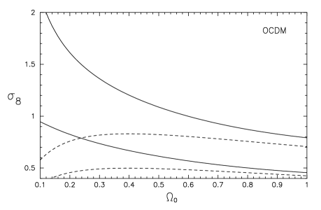
Figure 4: The cluster constraint (solid) is compared with the COBE normalization (dashed) for the range of $\Gamma$ satisfying the galaxy correlation data. The upper figure shows the open case, and the lower one the flat case. In each, it is assumed that all the dark matter is cold. The upper COBE line corresponds to $\Gamma=0.27$ and the lower one to $\Gamma=0.20$. Both cluster and COBE constraints are at 95 per cent confidence. The central values are not shown.

We do not intend a detailed comparison of these results with other types of observation here (see Liddle et al. 1995, 1996a, 1996b), but it is worth comparing the results with the normalization from the four-year COBE observations [Bennett et al. 1996, Banday et al. 1996, Górski et al. 1996, Hinshaw et al. 1996] for the case of scale-invariant ($n=1$) initial density perturbations. These fix the amplitude of perturbations on large scales, $\delta_{{\rm H}}^{2}$ as a function of $\Omega_{0}$, independently of $h$ to an excellent approximation. Fitting functions have been calculated by Bunn & White (in preparation) using techniques from White & Bunn [White & Bunn 1995], and are

$$10^{10}\delta_{{\rm H}}^{2}(\Omega_{0}) = 3.80\,\Omega_{0}^{-0.70-0.38\ln\Omega_{0}}\quad{\rm(OCDM)}\,;$$ (50)

$$10^{10}\delta_{{\rm H}}^{2}(\Omega_{0}) = 3.76\,\Omega_{0}^{-1.57-0.10\ln\Omega_{0}}\quad{\rm(}\Lambda{\rm CDM)}\,.$$ (51)

The fitting functions are accurate within about 3 per cent for $0.2<\Omega_{0}<1.0$. The COBE normalization error bar on $\delta_{{\rm H}}$ is 15 per cent at 2$\sigma$.

Although these values are independent of $h$, and indeed of the nature of the dark matter, they pick up a dependence on these when one computes the equivalent $\sigma_{8}$. We shall assume that the dark matter is all cold, so that we can use the $\Gamma$ parametrization of the transfer function. The uncertainty in the observed value of $\Gamma$ given after equation (5) propagates to the calculated value for $\sigma_{8}$ when one uses the appropriate COBE normalization for some value of $\Omega_{0}$. We will therefore add in quadrature the uncertainty thus arising in $\sigma_{8}$ and the 15 per cent error at 2$\sigma$ which appears in $\sigma_{8}$ due to the COBE normalization uncertainty.

The comparison is plotted in Fig. 4. The allowed range of values for $\Omega_{0}$ goes down to about 0.20 in the OCDM case. In the $\Lambda$CDM case the cluster constraint remains compatible with COBE and the galaxy correlation function shape down to very low $\Omega_{0}$. However, in this latter case there are other reasons for believing that low values are not favoured, for example, values of $\Omega_{0}$ below 0.4 require an anti-bias for optically selected galaxies due to their very high COBE normalization. This is difficult to understand physically. The anti-bias of IRAS galaxies would be even more pronounced. However, this conclusion is driven by COBE rather than the cluster abundance and can perhaps be partly alleviated by tilting the primordial spectrum.

For completeness, in Fig. 5 we show the comoving number density per unit temperature interval of clusters with mean X-ray temperature 7 keV that we should expect to observe at redshift $z$, for three cosmological models normalized to the present central value. The Sasaki and Lacey & Cole methods give very similar results. Note that these are clusters which have that temperature at the given redshift; their X-rays would be redshifted on the way to us, hence making the apparent temperature smaller by a factor of $(1+z)$. As one progresses to a lower redshift, some of the clusters will merge and some new ones will form. At present the only complete surveys of clusters at high redshifts are flux-limited (e.g. Henry, Jiao & Gioia 1994). This poses various problems, the most serious of which is that as the cluster selection is then a function of their luminosity, not of their temperature, we need to know the temperature–luminosity relationship at the appropriate redshift to be able to compare the observations with our results. However, this relation is very sensitive to several parameters like the cluster baryon fraction and the extent to which energy is injected into or removed from the intracluster medium, examples of the former being gas stripping from galaxies infalling into the cluster or supernova explosions in cluster galaxies, and of the latter being cooling flows.

Figure 5: The expected comoving number density of clusters for a unit temperature interval about 7 keV at redshift $z$ for three cosmological models: a critical-density universe (solid), an open universe with $\Omega_{0}=0.3$ (dashed) and a flat model with $\Omega_{0}=0.3$ (dotted). Each curve is normalized to produce the same present number density. The upper panel shows the result using the Sasaki merger calculation, and the lower one that of Lacey & Cole.

To recap on our main results, we have used a new method to compute the power spectrum constraint arising from the observed number density of clusters with a given X-ray temperature. We have done this for a critical-density universe and for both flat and open low-density universes. Although we have assumed that all the dark matter is cold, the constraint would not change much [Liddle et al. 1996b] if one went, for example, to a cold plus hot dark matter model. In cases where such calculations have been done previously, we support the previous results but typically find larger accumulated uncertainties.

For the case of pure cold dark matter, we have also compared our results with constraints from COBE and from the galaxy correlation function (which constrains the shape parameter $\Gamma$). We found that the cluster constraint is compatible with these in both the flat and open cases for any reasonable value of the density, failing only in the open case for $\Omega_{0}<0.20$. However, near critical density the corresponding $h$ will be very low (below 0.5), and at the lowest permitted densities it will be very high (above 1.0). Further, in the spatially flat case the concordance of these constraints at low values of $\Omega_{0}$ will require optically selected galaxies to be anti-biased with respect to the dark matter distribution.

References

- [Bahcall & Cen 1992] Bahcall N. A., Cen R., 1992, ApJ, 398, L81
- [Bahcall & Cen 1993] Bahcall N. A., Cen R., 1993, ApJ, 407, L49
- [Balland & Blanchard 1995] Balland C., Blanchard A., 1995, A&A, 298, 323
- [Banday et al. 1996] Banday A. J. et al., 1996, COBE preprint, astro-ph/9601065
- [Bardeen et al. 1986] Bardeen J. M., Bond J. R., Kaiser N., Szalay A. S., 1986, ApJ, 304, 15
- [Bartlett & Silk 1993] Bartlett J. G., Silk J., 1993, ApJ, 407, L45
- [Bennett et al. 1996] Bennett C. L. et al., 1996, COBE preprint, astro-ph/9601067
- [Bernardeau 1994] Bernardeau F., 1994, ApJ, 427, 51
- [Blain & Longair 1993a] Blain A. W., Longair M. S., 1993a, MNRAS, 264, 509
- [Blain & Longair 1993b] Blain A. W., Longair M. S., 1993b, MNRAS, 265, L21
- [Bond & Myers 1992] Bond J. R., Myers S. T., 1992, in Cline D., Peccei R., eds, Trends in Astroparticle Physics. World Scientific, Singapore, p. 262
- [Bond et al. 1991] Bond J. R., Cole S., Efstathiou G., Kaiser N., 1991, ApJ, 379, 440
- [Carroll et al. 1992] Carroll S. M., Press W. H., Turner E. L., 1992, ARA&A, 30, 499
- [Charlton & Turner 1987] Charlton J. C., Turner M. S., 1987, ApJ, 313, 495
- [Colafrancesco & Vittorio 1994] Colafrancesco S., Vittorio N., 1994, ApJ, 422, 443
- [Edge et al. 1990] Edge A. C., Stewart G. C., Fabian A. C., Arnaud K. A., 1990, MNRAS, 245, 559
- [Efstathiou, Sutherland & Maddox 1990] Efstathiou G., Sutherland W. J., Maddox S. J., 1990, Nat, 348, 705
- [Eke, Cole & Frenk 1996] Eke V. R., Cole S., Frenk C. S., 1996, Durham preprint, astro-ph/9601088
- [Evrard 1989] Evrard A. E., 1989, ApJ, 341, L71
- [Górski et al. 1995] Górski K. M., Ratra B., Sugiyama N., Banday A. J., 1995, ApJ, 444, L65
- [Górski et al. 1996] Górski K. M. et al., 1996, COBE preprint, astro-ph/9601063
- [Hanami 1993] Hanami H., 1993, ApJ, 415, 42
- [Henry & Arnaud 1991] Henry J. P., Arnaud K. A., 1991, ApJ, 372, 410
- [Henry, Jiao & Gioia 1994] Henry J. P., Jiao L., Gioia I. M., 1994, ApJ, 432, 49
- [Hinshaw et al. 1996] Hinshaw G. et al., 1996, COBE preprint, astro-ph/9601058
- [Kaiser & Squires 1993] Kaiser N., Squires G., 1993, ApJ, 404, 441
- [Klypin, Primack & Holtzman 1995] Klypin A., Primack J., Holtzman J., 1995, NMSU preprint, astro-ph/9510042
- [Kofman, Gnedin & Bahcall 1993] Kofman L. A., Gnedin N. Y., Bahcall N. A., 1993, ApJ, 413, 1
- [Kolb & Turner 1990] Kolb E. W., Turner M. S., 1990, The Early Universe. Addison-Wesley, Redwood City, California, p. 53
- [Lacey & Cole 1993] Lacey C., Cole S., 1993, MNRAS, 262, 627
- [Lacey & Cole 1994] Lacey C., Cole S., 1994, MNRAS, 271, 676
- [Liddle & Lyth 1993] Liddle A. R., Lyth D. H., 1993, Phys. Rep., 231, 1
- [Liddle et al. 1995] Liddle A. R., Lyth D. H., Viana P. T. P., White M., 1995, Sussex preprint, astro-ph/9512102
- [Liddle et al. 1996a] Liddle A. R., Lyth D. H., Roberts D., Viana P. T. P., 1996a, MNRAS, 278, 644
- [Liddle et al. 1996b] Liddle A. R., Lyth D. H., Schaefer R. K., Shafi Q., Viana P. T. P., 1996b, to appear MNRAS, astro-ph/9511057
- [Lilje 1992] Lilje P. B., 1992, ApJ, 386, L33
- [Martel 1991] Martel H., 1991, ApJ, 477, 7
- [Metzler & Evrard 1994] Metzler C. A., Evrard A. E., 1994, ApJ, 437, 564
- [Monaco 1995] Monaco P., 1995, ApJ, 447, 23
- [Navarro et al. 1995] Navarro J. F., Frenk C. S., White S. D. M., 1995, MNRAS, 275, 720
- [Oukbir & Blanchard 1992] Oukbir J., Blanchard A., 1992, A&A, 262, L21
- [Peacock 1996] Peacock J. A., 1996, Edinburgh preprint, astro-ph/9601135
- [Peacock & Dodds 1994] Peacock J. A., Dodds S. J., 1994, MNRAS, 267, 1020
- [Peacock & Heavens 1990] Peacock J. A., Heavens A. F., 1990, MNRAS, 243, 133
- [Press & Schechter 1974] Press W. H., Schechter P., 1974, ApJ, 187, 452
- [Ratra & Peebles 1994] Ratra B., Peebles P. J. E., 1994, ApJ, 432, L5
- [Sasaki 1994] Sasaki S., 1994, PASJ, 46, 427
- [Sugiyama 1995] Sugiyama N., 1995, ApJS, 100, 281
- [White & Bunn 1995] White M., Bunn E. F., 1995, ApJ, 450, 477
- [White et al. 1993a] White S. D. M., Efstathiou G., Frenk C. S., 1993a, MNRAS, 262, 1023
- [White et al. 1993b] White S. D. M., Navarro J. F., Evrard A. E., Frenk C. S., 1993b, Nat, 366, 429