Applications of Minkowski-Functionals to the Statistical Analysis of Dark Matter Models

Abstract

A new method for the statistical analysis of 3-D point processes, based on the family of Minkowski-Functionals , is explained and applied to modelled galaxy distributions generated by a toy-model and cosmological simulations of the large-scale structure in the Universe. These measures are sensitive to both, geometrical and topological properties of spatial patterns and appear to be very effective in discriminating different point processes. Moreover by the means of conditional subsampling, different building blocks of large-scale structures like sheets, filaments and clusters can be detected and extracted from a given distribution.

1 Introduction

The still unsolved question of the origin and evolution of the Large-Scale Structure (LSS) of the universe is a central topic in modern cosmology. The scientific approach to this problem is based on three columns:

1. The distribution of matter in the Universe is assumed to be traced by luminous galaxies. Thus, observation of galaxies and measurement of their redshifts is, besides peculiar–velocity measurements, the only way to gain an idea of the matter distribution in our local area of the Universe.

2. Todays powerful computer systems make the numerical simulation of statistical ensembles of theoretical models of structure formation possible. By this way effects of different dark matter models on the resulting structures can be studied.

3. The comparison of observations with theoretical models is made in terms of statistical measures which can be applied to both, real and simulated galaxy distributions. Thus, models can either be sorted out or favoured and improved to fit observational results.

The introduced statistical method belongs to the third column and offers a new approach for finding adequate measures which are capable of discribing and characterizing global and local features of galaxy distributions. It was first suggested by Mecke, Buchert and Wagner [8], but only now numerical problems are overcome and first results can be gained.

Popular measures in that field include N-Point Correlation Functions [9], Counts-in-Cells [2], Void Probability Functions [12], Percolation Analysis [13], Minimal Spanning Trees [1], Genus of Isodensity Levels [3], Voronoi-foam Statistics [5, 11] and many more.

After discussing the basic properties of Minkowski-Functionals in Section 2, the new statistical method is presented in Section 3. Its sensitivity to different components of the LSS (clusters, walls, filaments) is investigated, using toy-models based on Voronoi-tesselations, and the selection of structures by the means of conditional subsampling is illustrated (Section 4). Finally the method is applied to a series of CDM-simulations in Section 5, a short summary is given in Section 6, and an outlook on future prospects in Section 7.

2 Minkowski-Functionals

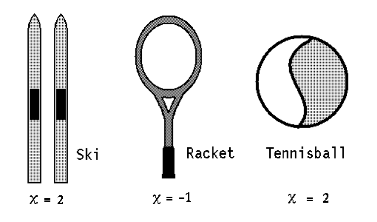
The Minkowski-Functionals $W_{\nu}$ have their origin in the mathematical theory of convex bodies and integral geometry. In $d$ dimensions there exist $d+1$ of these functionals including geometrical and topological descriptors to characterize content (volume and surface), shape and connectivity of a body $A\subset\mbox{\rm I\kern-1.79993ptR}^{d}$ :

In the case of three dimensions we have:

$\begin{array}[]{rcll}W_{0}&=&V(A)&\quad\mbox{(volume)}\\ 3W_{1}&=&S(A)&\quad\mbox{(surface)}\\ 3W_{2}&=&H(A)&\quad\mbox{(shape)}\\ 3W_{3}&=&G(A)\\ &=&4\pi\raisebox{2.27626pt}{\mbox{$\chi\ $}}(A)&\quad\mbox{(connectivity)}\\ \end{array}$

Here, shape is expressed in terms of the integral mean curvature $H$ of a body’s surface, and the integral Gaussian curvature $G$, related to the Euler-characteristic $\chi$ via the Gauß-Bonnet theorem, is a measure for the connectivity.

Important properties of the Minkowski-Functionals include:

Motion Invariance :	$\mbox{$W_{\nu}$}(uA)$	=	$\mbox{$W_{\nu}$}(A)$
Additivity :	$\mbox{$W_{\nu}$}(A\cup B)$	=	$\mbox{$W_{\nu}$}(A)+\mbox{$W_{\nu}$}(B)-\mbox{$W_{\nu}$}(A\cap B)$

Thus, the measures are invariant against translations and rotations of the body or combinations $u$ of the two. The $W_{\nu}$ of a body $C$, which is the union of two point sets $A$ and $B$, obey a simple additivity relation that can be extended by induction to an arbitrary number of components of $C$. Except for the volume, all other measures are located on the surface of the considered body.

Euler-characteristic

The Euler-characteristic $\raisebox{2.27626pt}{\mbox{$\chi\ $}}=G/4\pi$ of a body $A$ is related to its genus $g$

$$\raisebox{2.27626pt}{\mbox{$\chi\ $}}(A)=1-g(A)\;\;,$$

so in three dimensions $\chi\$can be expressed by :

$$\raisebox{2.27626pt}{\mbox{$\chi\ $}}=components-tunnels+cavities\;\;.$$

In this way it can be used as a topological measure for the connectivity of a point set.

Figure 1: Example: A pair of ski consists of two components and, unless there are holes or cavities inside a ski, an Euler-characteristic of $\chi=2$ is found. The tennis racket has two ”tunnels” and one component yielding $\chi=-1$ (however, a more realistic one would have a highly negative $\chi$). Finally a tennis ball has a cavity and thus $\chi=2$.

3 Method

3.1 Boolean Grain Model

Figure 2: Each point is decorated with a ball $B_{r}$.

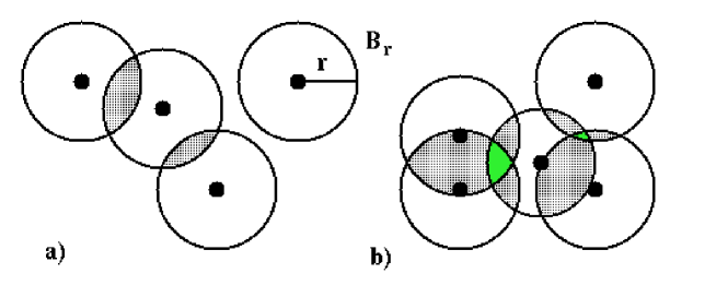
In a given distribution the points (galaxies) are represented by their cartesian coordinates $\vec{x}_{i}$. The input data are the coordinates of all the $N$ points inside a cubic volume $\cal C$ that is cut out of the point distribution. This cube is then scaled to an edgelength of one (unit cube ${\cal C}_{u}$). Outside this box periodic boundary conditions are used, i.e. ${\cal C}_{u}$ is supplemented by 26 identical boxes around it. For the calculations, on every point a ball $B_{r}$ with radius $r$ is centered (Boolean grain model).

The Minkowski measures of the point set ${\cal B}(r)=\cup_{i=1}^{N}B_{r}(\vec{x}_{i})$ which consists of all the points inside the union of the balls are then calculated, partly using numerical methods. Actually the local contributions $\mbox{$W_{\nu}$}(r,\vec{x}_{i})$ to the functionals from the surface of each single ball $B_{r}(\vec{x}_{i})$ (i=1,…,N) are determined and global measures arise by taking the mean of all the $\mbox{$W_{\nu}$}(r,\vec{x}_{i})$ for a given radius $r$. It can be shown that these global results contain $n$-point correlations of every order $n$.

The radius $r$ of the balls is the parameter that is needed to analyze the distribution on different scales. For small radii most of the balls are isolated, thus yielding the measures of a ball ($\raisebox{2.27626pt}{\mbox{$\chi\ $}}=1$). With growing $r$ more and more balls intersect and connect to network-like structures ($\raisebox{2.27626pt}{\mbox{$\chi\ $}}<0$). Finally, the network turns into a body with enclosed cavities ($\raisebox{2.27626pt}{\mbox{$\chi\ $}}>0$) which then are filled when the cube ${\cal C}_{u}$ ist totally overlapped by ${\cal B}(r)$.

Figure 3: Boolean grain model for a Poisson process for two values of $r$, corresponding to ($x=r/{<D>}$) $x_{1}=0.18$ (left) and $x_{2}=0.36$ (right); $<D>$ is the mean distance of points in the set.

3.2 Results for Poissonian Sample

The mean values of the Minkowski-Functionals can be calculated analytically for a stationary Poisson process [6]. The radius is scaled by the mean distance $<d>$ between the points in the cube ${\cal C}_{u}$.

Figure 4: Global MF per ball (analytical).

Figure 5: The distribution of the local Euler-characteristic.

4 Analysis of Toy Models

4.1 Voronoi Tesselations

A toy model for the artificial generation of structures, roughly similar in to the ones observed in the Universe, is based on Voronoi Tesselations:

Figure 6: (from [11]) A Voronoi-Tesselation is a decomposition of space into convex, non-overlapping domains, which are generated as Wigner-Seitz cells of a discrete distribution of points;
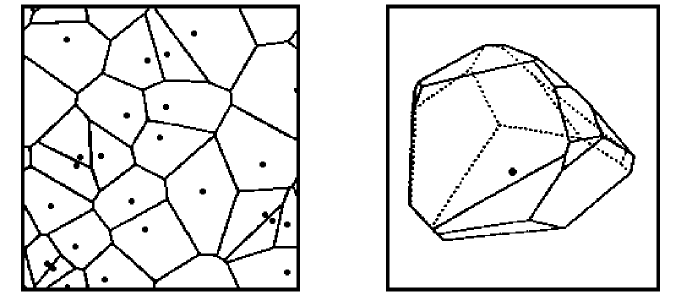
a) Voronoi-Tesselation in two dimensions, b) example for a cell and its nucleus (d=3).

A Poissonian distribution of points (”nuclei”) inside ${\cal C}_{u}$ defines a pattern of Wigner-Seitz-cells, the tesselation. In a second step a number of $N$ test-points is randomly distributed inside ${\cal C}_{u}$. Then these points are projected onto the walls, or edges, or vertices of the tesselation, thus generating sheets (or walls), filaments or clusters. For all these structure components one can choose a finite thickness and the ratio of points ending up in each of them.

4.2 Walls, Filaments and Clusters

The method is sensitive to different structures in a distribution of points. This can be illustrated by looking at the local contributions to the Euler-characteristic $\chi\$on the surface $S$ of each ball. As $\chi\$is equivalent to the integrated Gaussian curvature of the considered body, it can be split into three contributions[8], coming from the uncovered surface ($\chi_{Sur}$), the intersection lines ($\chi_{Lin}$) of two balls on $S$ and the triplepoints ($\chi_{Tri}$) where three balls have a common point on $S$. Surface points, that belong to more than three balls have a low probability and can be neglected.

While for walls, $\chi\$includes contributions from lines and triplepoints over a wide range of $x$, hardly any triplepoints appear for filaments. The Euler-characteristic $\chi\$has a narrow minimum for clustered distributions, but no distinct minimum for filaments.

Figure 7: Local contributions to $\chi$ from the surface ($\chi_{Sur}$), the intersection lines ($\chi_{Lin}$) and the triplepoints ($\chi_{Tri}$); ($x=r/{<D>}$).

4.3 Conditional Subsampling

Structures can be detected and analyzed by selecting only galaxies with a local contribution to a functional inside a given interval.

As an example we consider a mixture of filaments ($4000$ points) generated in the Voronoi model and a Poissonian distribution (also $4000$ points). We can extract the filament component by suitable conditions on the local contributions to the Minkowski-Functionals: Typical for filaments, e.g., is $\chi\approx 0$ (see Figure 7and Figure 8); we have chosen the condition $-0.1\leq\raisebox{2.27626pt}{\mbox{$\chi\ $}}\leq 0.1$.

Figure 8: Original distribution, filament component and two selected samples at different radii $r$ (corresponding to ($x=r/{<D>}$) $x_{1}=0.28\;;x_{2}=0.48$. The first selection consists of about $2000$ points with more than 88% of them belonging to filaments. The second has 3400 points with 70% in filaments. The pictures show all points of the samples projected onto the x–y plane of the cube ${\cal C}_{u}$.

4.4 Two-point distributions with similar two-point correlations

Figure 9: The quotient of $\chi\$and the uncovered ratio of the surface $S$ is a good measure to discriminate the two distributions $1$ and $2$ having similar 2-point correlation functions $\xi(x)$ on scales smaller than $x_{0}$: $\xi(x_{0})=1$. The error bars shown are the standard deviations of the mean of the ball contributions in each sample.

5 Analysis of CDM-Simulations

Figure 10: $k^{n}$ power spectra with n = 0, -1, -1,5 [S.D.M.White, priv.comm.] 10000 points (out of $10^{6}$) plotted for each sample

The results show clearly the different reaction of the Minkowski-Functionals to the three spatial patterns. For a constant power spectrum $\propto k^{0}$ many small clusters can form, while for negative $n$ bigger structures appear. In the case of $n=0$ the ratio of galaxies in clusters is higher than for $n<0$, so the volume and surface measures yield lower values, while the mean curvature remains positive. For negative $n$ the points outside of clusters are part of a network generated by the corresponding balls in the grain model, thus adding high surface contributions and negative curvature values (curvature of intersection lines $H_{Lin}<0$ !).

Figure 11: Minkowski-Functionals for CDM simulations with $k^{n}$ power spectra; ($x=r/{<D>}$).

6 Conclusions

The introduced statistical method is based on a solid mathematical background and no special assumptions about the sample have to be made. The mean values of the functionals over the balls in a sample are statistically unbiased descriptors and include topological and geometrical measures, containing n-point correlations of every order[8]. They are statistically robust even for small samples and depend on the radius of balls which is the (single) diagnostic parameter in the Boolean grain model. The method is efficient in discriminating spatial patterns and selecting structures by the means of conditional subsampling.

7 Outlook

The calculation of the family of Minkowski–Functionals by using a Boolean model of penetrable grains and evaluating the local (per grain) contributions to the functionals $W_{\nu\;;\;\nu\geq 1}$ on the surface of the overlapping union of grains is an effective way of characterizing the local as well as the global morphology of point processes, as we have just shown.

As a result of the local calculation of the contributions to the MF’s, this method offers a variety of different informations by conditional subsampling and by using various combinations of MF’s. The latter is necessary as noted earlier [14]: the Euler characteristic alone is not a preferable tool to discriminate similar point processes (compare Fig.2 left and right panels in [14] and Fig.11). In addition, geometrical information is needed, which is furnished by the other MF’s. Only all $4$ measures can (within the class of additive and motion invariant measures) completely characterize the morphology.

The current numerical code to calculate the MF’s performs with reasonable storage and CPU time (we need about 180–250 MB storage and 1–6 h CPU time, depending on machine and degree of clustering, to realize, e.g., a sample of $10^{6}$ points).

In our statistics group (SFB 375/B3) we currently work on an alternative way to calculate the MF’s: We use a grid and calculate the MF’s by their contributions per grid cell on a sufficiently fine grid spacing. The resulting code is comparatively fast and storage efficient. Moreover, it implies another advantage: in addition to point samples we can consider density– or temperature fields (given on a grid) which renders the method applicable to smoothed cosmic density fields and microwave background maps. Smoothing is another key–element of this method which defines one of our near future perspectives.

We envisage two steps:

1. We calculate the MF’s of smoothed fields (employing, e.g. Gaussian filters). Introducing a second diagnostic parameter (e.g. a density threshold), this method covers the topology approach by Gott, Melott, Weinberg and collab. (see: [17] and ref. therein), where we use $4$ functionals instead of just one. We here try to restore motion invariance (with respect to the discrete group of motions) and additivity, two important properties to allow for a local characterization of morphology. This method will also cover the topological/geometrical approach on a grid introduced in [18].

2. We will combine, so–called Koenderink measures ([15],[16],[19]) with MF’s. Koenderink measures provide a set of specific filters which extract different pattern recogition elements from a smoothed point set. For different smoothing lengths the performance of these filters displays an optimum on some smoothing scale.

The combination of these methods will provide a powerful tool for the morphological characterization of point processes, density– and temperature fields in scale–space.

A further perspective concerns stereological applications of MF’s (see, e.g., [20]), i.e., the possibility of extracting 3D informations from lower–dimensional data sets (such as pencil beam surveys). It will be necessary to analyse smoothed and unsmoothed Minkowski–measures in the three–dimensional space compared with those in projected distributions.

Acknowledgments:

We would like to thank Rien van de Weygaert for providing his Voronoi tesselation code, and Simon White for providing his N–body simulation results; we have benefited from numerous discussions with them and with Gerhard Börner, Stefan Gottlöber, Martin Kerscher, Houjun Mo, Jens Schmalzing and Herbert Wagner.

TB is supported by the ”Sonderforschungsbereich 375–95 für Astro–Teilchenphysik” der Deutschen Forschungsgemeinschaft.