Open cold dark matter models

Abstract

Motivated by recent developments in inflationary cosmology indicating the possibility of obtaining genuinely open universes in some models, we compare the predictions of cold dark matter (CDM) models in open universes with a variety of observational information. The spectrum of the primordial curvature perturbation is taken to be scale invariant (spectral index $n=1$), corresponding to a flat inflationary potential. We allow arbitrary variation of the density parameter $\Omega_{0}$ and the Hubble parameter $h$, and take full account of the baryon content assuming standard nucleosynthesis. We normalize the power spectrum using the recent analysis of the two year COBE DMR data by Górski et al. We then consider a variety of observations, namely the galaxy correlation function, bulk flows, the abundance of galaxy clusters and the abundance of damped Lyman alpha systems. For the last two of these, we provide a new treatment appropriate to open universes. We find that, if one allows an arbitrary $h$, then a good fit is available for any $\Omega_{0}$ greater than 0.35, though for $\Omega_{0}$ close to 1 the required $h$ is alarmingly low. Models with $\Omega_{0}<0.35$ seem unable to fit observations while keeping the universe over $10$ Gyr old; this limit is somewhat higher than that appearing in the literature thus far. If one assumes a value of $h>0.6$, as favoured by recent measurements, concordance with the data is only possible for the narrow range $0.35<\Omega_{0}<0.55$. We have also investigated $n\neq 1$; the extra freedom naturally widens the allowed parameter region. Assuming a range $0.9<n<1.1$, the allowed range of $\Omega_{0}$ assuming $h>0.6$ is at most $0.30<\Omega_{0}<0.60$.

1 Introduction

Even before the announcement of the detection of microwave background anisotropies by the DMR experiment on the COBE satellite [Smoot et al. 1992], it was realized that structure formation models based on cold dark matter (CDM) and a flat spectrum of primordial perturbations fared considerably better against the data if the matter density was reduced by a factor of around three. Most studies of this possibility invoked a cosmological constant to restore spatial flatness [Efstathiou, Sutherland & Maddox 1990, Kofman, Gnedin & Bahcall 1993], with little attention being directed to the possibility that the cosmological constant may be redundant and the low-density model implemented in a genuinely open universe. This produces the same shape of perturbation spectrum on scales well below the curvature radius, but a different normalization and redshift dependence.

The reluctance to study such models (though general arguments in favour of an open universe were developed, e.g. Coles & Ellis [Coles & Ellis 1994] and Primack [Primack 1995]) arose from a widespread belief that inflation, the most plausible candidate for generating the initial density perturbations, could give rise to an open universe only in exceptionally fine-tuned circumstances. However, open universe inflation models have received renewed interest recently, and in particular attention has been drawn (Sasaki et al. 1993a, 1993b; Tanaka & Sasaki 1994; Bucher, Goldhaber & Turok 1995; Yamamoto, Sasaki & Tanaka 1995a; Sasaki, Tanaka & Yamamoto 1995; Yamamoto, Tanaka & Sasaki 1995b; Bucher & Turok 1995) to the bubble nucleation model [Coleman & de Luccia 1980, Gott 1982, Guth & Weinberg 1983, Gott & Statler 1984, Linde 1995, Amendola, Baccigalupi & Occhionero 1995]. In contrast with the situation for ordinary models of inflation [Lyth & Stewart 1990a, Ratra & Peebles 1995], this model predicts the present value of the density parameter in terms of the scalar field potential, without any reference to initial conditions. The price that one pays for this is a non-generic scalar field potential, which will be even more difficult than usual to realize in the context of a sensible particle physics model.

In order to compare structure formation models based on open universe inflation models with observational data, it is crucial to be able to normalize the amplitude of the power spectrum to the COBE observations of cosmic microwave background (CMB) fluctuations [Bennett et al. 1994], which are by far the most accurate available. Anisotropy calculations in an open universe present many technical difficulties and progress to the result has consequently been slow. However, an accurate normalization is now available through the work of Górski et al. (1995, henceforth GRSB), superseding earlier versions by Ratra & Peebles [Ratra & Peebles 1994] and by Kamionkowski et al. [Kamionkowski et al. 1994].

The viability of the open CDM model has recently been investigated by Ratra & Peebles [Ratra & Peebles 1994]. This paper predated the improved normalizations of inflationary open models to COBE supplied first by Kamionkowski et al. [Kamionkowski et al. 1994] and then more accurately again by GRSB (see also White & Bunn 1995). Each of those collaborations provided only a brief account of the model’s status against observations other than those of the microwave background. It is our aim in this paper to make a more extensive comparison of the model with observations.

2 The Open Universe Power Spectrum

The model is defined by giving the spectrum ${\cal P}(k)$ of the density contrast $\delta$. Our approach towards constraining the model is to utilize linear perturbation theory, applied across as wide a range of scales as possible. By considering the formation of objects such as quasars and damped Lyman alpha systems at moderate redshift, it is possible to impose constraints on the spectrum at scales down to one megaparsec or less, while COBE probes scales of several thousands of megaparsecs, up to and even above the curvature scale. Between these extremes, a variety of different constraints can be applied.

All of the observations except the CMB anisotropy probe scales which are small compared with the Hubble distance, so we can use the Newtonian description of density perturbations to describe them. At any epoch well after matter domination sets in, the power spectrum of the density contrast is

$${\cal P}(k)=\delta_{H}^{2}T^{2}(k)\frac{g^{2}(\Omega)}{g^{2}(\Omega_{0})}\left(\frac{k}{aH}\right)^{4}\,.$$ (1)

Here $a$ is the scale factor of the universe, $H=\dot{a}/a$ is the Hubble parameter (dots signifying time derivatives), $k$ is the comoving wavenumber (in inverse megaparsecs) and we are defining ${\cal P}(k)$ as the power per unit logarithmic interval of $k$. The transfer function $T(k)$ specifies the scale-dependent effect of the evolution of the density perturbation between horizon entry and matter domination, and is normalized to unity on large scales. The factor $g(\Omega)$ is introduced to allow for the growth law for perturbations in an open universe. It gives the total suppression of growth in an open universe relative to a critical density universe, and is accurately given by the fitting function [Carroll, Press & Turner 1992]

$$g(\Omega)=\frac{5}{2}\Omega\left[1+\frac{\Omega}{2}+\Omega^{4/7}\right]^{-1}\,.$$ (2)

Finally, the quantity $\delta_{H}$ specifies the overall normalization of the present-day spectrum. Its independence of $k$ indicates the assumption of an inflationary model leading to a scale-invariant spectrum; in typical inflationary models one would expect some deviation from this [Liddle & Lyth 1993] and we shall consider this at the end of the paper. Inflationary models also predict the existence of gravitational waves, but their effect on the COBE normalization has not yet been successfully calculated and so we assume they are negligible. The value of $\delta_{H}$, when fixed by the COBE observations as discussed below, depends on $\Omega_{0}$, but it has only an extremely weak dependence on $H_{0}$ which can be comfortably ignored (throughout, a subscript 0 denotes the present day).

Many observations do not allow one to impose constraints on the power spectrum itself, but instead place constraints on the dispersion of the density contrast $\sigma(R)$ smoothed on a comoving scale $R$. We shall always use a top-hat filter $W(kR)$ defined by

$$W(kR)=3\left(\frac{\sin(kR)}{(kR)^{3}}-\frac{\cos(kR)}{(kR)^{2}}\right)$$ (3)

to perform the smoothing. The dispersion of the smoothed density contrast is easily calculated from a theoretical power spectrum as

$$\sigma^{2}(R)=\int_{0}^{\infty}{\cal P}(k)\,W^{2}(kR)\,\frac{{\rm d}k}{k}\,.$$ (4)

The prediction for the abundance of objects of various types has a very simple interpretation as a constraint on $\sigma(R)$, which cannot be easily represented as a power spectrum constraint.

Before proceeding to a full account of the data and their interpretation, let us be more specific regarding our assumptions. The parameters that we shall consider as freely variable are the total present density $\Omega_{0}$ and the present Hubble parameter $h$ (in units of $100\;{\rm km}\,{\rm s}^{-1}\,{\rm Mpc}^{-1}$). An important contribution to be taken into account is the baryonic component of the density, $\Omega_{{\rm B}}$, which we take to be fixed by nucleosynthesis as $\Omega_{{\rm B}}h^{2}=0.0125$ [Walker et al. 1991]. In the presence of baryons, the usual scaling law of the transfer function with $\Omega_{0}h$ (which is exact only for zero baryon density) can be replaced by an empirical scaling law with $\Omega_{0}h\exp(-\Omega_{{\rm B}}-\Omega_{{\rm B}}/\Omega_{0})$. This law was discovered by Sugiyama [Sugiyama 1994], and generalizes a scaling law advertised by Peacock & Dodds [Peacock & Dodds 1994] to the case where $\Omega_{0}<1$. Although Sugiyama’s calculations were made for the case of a flat universe with a cosmological constant, the difference between that and the present case only sets in long after the universe is matter dominated and so the shape is the same in our case. The different overall normalization of the spectrum between the two cases is of course included in the COBE normalization that we shall carry out.

We use the transfer function from Bardeen et al. [Bardeen et al. 1986],

$$T_{{\rm CDM}}(q) = \frac{\ln\left(1+2.34q\right)}{2.34q}\times$$

$$\left[1+3.89q+(16.1q)^{2}+(5.46q)^{3}+(6.71q)^{4}\right]^{-1/4}\,,$$

with $q=k/h\Gamma$, where the so-called ‘shape parameter’ $\Gamma$ is defined as

$$\Gamma=\Omega_{0}h\exp(-\Omega_{{\rm B}}-\Omega_{{\rm B}}/\Omega_{0})\,,$$ (6)

in accordance with Sugiyama [Sugiyama 1994] as discussed above.

Although $h$ is in principle freely variable, it is determined at some level of accuracy by the requirement of a reasonable fit to the galaxy correlation function (see further discussion below), which demands that $\Gamma$ should lie in the range $[0.22,0.29]$ at 95 per cent confidence level assuming a scale-invariant power spectrum [Peacock & Dodds 1994]. Note though that, as $\Omega_{0}$ tends to 1, the required value of $h$ to achieve this begins to get uncomfortably small.

Particularly for high $h$, one is in danger of a conflict between measured ages of stellar populations and the age of the universe. In an open universe the age is given by

$$t_{0}=\frac{1}{\Omega_{0}H_{0}}\left[\frac{\Omega_{0}}{1-\Omega_{0}}-\frac{\Omega_{0}^{2}}{2\left(1-\Omega_{0}\right)^{3/2}}\cosh^{-1}\left(\frac{2-\Omega_{0}}{\Omega_{0}}\right)\right].$$ (7)

If one fixes $H_{0}$, then higher ages are achieved by lowering $\Omega_{0}$. However, we have written it this way to emphasize an alternative view, which is that the galaxy correlation function more or less fixes (ignoring for now the baryonic corrections) the combination $\Omega_{0}H_{0}$. Then the quantity in square brackets in the above formula is actually an increasing function of $\Omega_{0}$, peaking at $2/3$ when $\Omega_{0}=1$. Consequently, at fixed $\Gamma$, the desire for a large age favours a larger value of $\Omega_{0}$. To make this concrete, then fixing $\Gamma=0.25$ taking the baryons into account gives the sample values $\Omega_{0}=0.2\Rightarrow h=1.3\Rightarrow\;{\rm Age}\;=6$ Gyr; $\Omega_{0}=0.3\Rightarrow h=0.89\Rightarrow\;{\rm Age}\;=9$ Gyr; $\Omega_{0}=0.4\Rightarrow h=0.69\Rightarrow\;{\rm Age}\;=11$ Gyr; $\Omega_{0}=1.0\Rightarrow h=0.32\Rightarrow\;{\rm Age}\;=20$ Gyr. In each case the 15 per cent or so uncertainty in $\Gamma$ contributes a similar uncertainty to the age.

We shall adopt the extremely conservative view that the age should exceed $10$ Gyr, though there are many indications that the Universe is older (e.g. Demarque, Deliyannis & Sarajedini 1991; Stockton, Kellogg & Ridgway 1995) which one can use to constrain cosmological parameters without reference to large scale structure.

3 Normalization to COBE

The most crucial piece of data is the overall normalization of the density perturbation spectra, which we choose to match the microwave anisotropies at large angular scales measured by the DMR experiment on the COBE satellite [Bennett et al. 1994, Górski et al. 1994]. In the language of the usual spherical harmonic decomposition, COBE measures the multipoles with $l\la 30$, and for a given $\Omega_{0}$ the distance subtended at the surface of last scattering is comparable with the curvature if $l\la 2\sqrt{1-\Omega_{0}}/\Omega_{0}$. With the possible exception of the super-curvature modes defined below, this criterion gives an upper bound on the range of $l$ for which curvature can be significant. It may however be a considerable overestimate, because for $\Omega_{0}<1$ the dominant contribution to the CMB anisotropy can come from distances far closer than the surface of last scattering. In any case it allows curvature to affect only $l\la 6$ even for $\Omega_{0}$ as low as $0.3$, which means that at most the lowest few multipoles of COBE are likely to be sensitive to curvature.

To investigate the effect of curvature quantitatively, one must first ask how the Newtonian expression (1) should be continued to larger scales. As discussed in detail in Lyth & Woszczyna [Lyth & Woszczyna 1995], a number of issues have to be addressed.

First, in order to define the density contrast one has to specify a slicing of space-time into spatial hypersurfaces. We make the usual choice that the hypersurfaces are orthogonal to comoving observers, corresponding to what is called the ‘gauge invariant’ density perturbation. In the era well after matter domination (which is the only one that concerns us) this is the same as the ‘synchronous gauge’ density perturbation [Lyth & Stewart 1990b].

Secondly there is the definition of the spectrum. In discussing the stochastic properties of a given perturbation $f$, one assumes that it is a typical realization of a random field (an ensemble of functions together with a probability distribution for them). In both flat and curved space, the spectrum is defined with reference to an expansion in terms of eigenfunctions of the Laplacian, being the ensemble average of the modulus squared of the coefficient. Following Lyth & Stewart [Lyth & Stewart 1990a], we denote the eigenvalue of the Laplacian by $-(k/a)^{2}$, and normalize the spectrum ${\cal P}_{f}(k)$ of a generic perturbation $f$ so that it gives the power per unit logarithmic interval of $k$. (By ‘power’ we mean the ensemble mean square contribution to $f^{2}$, which is independent of position.) We are taking the random field to be Gaussian, which means that each coefficient has an independent Gaussian probability distribution, whose variance is essentially defined by the spectrum. (To make this statement precise one needs to take account of the fact that $k$ is a continuous, not a discrete, variable.)

Thirdly, there is the range of $k$ over which the spectrum is non-zero. If $k^{-1}$ is measured in units of the curvature scale $H_{0}^{-1}/\sqrt{1-\Omega_{0}}$, then it is known that the most general square integrable function can be constructed using only the eigenfunctions with $k^{2}>1$. For this reason, cosmologists have always assumed that the same is true for the most general Gaussian random field. That is, they have assumed that such a field can always be generated by keeping only the the sub-curvature modes (those with $0<k^{-2}<1$) as distinct from the super-curvature modes (those with $k^{-2}>1$). It has recently been pointed out [Lyth & Woszczyna 1995] that this is not so; rather, mathematicians have known for half a century that in order to construct the most general Gaussian random field the spectrum (and therefore the eigenfunction expansion) needs to run over the full range $k^{2}>0$. Such super-curvature modes can arise in the single-bubble models of open inflation [Yamamoto et al. 1995b], though as we shall see it is a reasonable working hypothesis to assume that the effect of these is negligible.

In most of the cosmology literature a different normalization of the spectrum is adopted, which is denoted by $P_{f}$ rather than by ${\cal P}_{f}$. In flat space, $P_{f}$ is normalized so that $k^{3}P_{f}/(2\pi^{2})$ is the power per unit logarithmic interval of $k$. Because super-curvature modes were never considered, this definition is customarily generalized to make $q^{3}P_{f}/(2\pi^{2})$ the power per unit logarithmic interval of $q$, where $q^{2}=k^{2}-1$. (The motivation for considering $q^{2}$ instead of $k^{2}$ is that its range is $q^{2}>0$.) This leads to the relation

$$P_{f}(q)=\frac{2\pi^{2}}{q(q^{2}+1)}{\cal P}_{f}(k(q))\,.$$ (8)

These preliminaries having been addressed, we are ready to ask what is the correct continuation to large scales of the flat space expression (1)? A natural choice is to keep equation (1) as it stands, either retaining or dropping the super-curvature modes. If super-curvature modes are dropped there are other natural choices, based on the alternatively defined spectrum $P$ that we have just discussed. One can take $P\propto q$ (the usual choice until recently) or $P\propto k$; these choices multiply equation (1) by $(q/k)^{2}$ and $q/k$ respectively. Another choice [Kamionkowski & Spergel 1994], relating to the density contrast smoothed over a sphere of variable radius, makes $P\propto q^{3}$ for $q\la 1$ going smoothly over to $P\propto q$ for $q\ga 1$.

A further possibility is that, instead of focusing on the density contrast $\delta$, one can focus on the primordial curvature perturbation $\cal R$, given by [Bardeen 1980, Lyth & Stewart 1990a]

$${\cal R}=\frac{5}{2}\left(\frac{a^{2}H^{2}}{3+k^{2}}\right)\delta\,.$$ (9)

On small scales equation (1) corresponds to a scale-independent spectrum ${\cal P}_{\cal R}$. However, if ${\cal P}_{\cal R}$ is taken to be scale independent on large scales also, equation (1) is multiplied by a factor $[(3+k^{2})/k^{2}]^{2}$. At $k^{2}=2$ this is a factor $\simeq 5$, corresponding to a factor $\sqrt{5}$ in the rms perturbation, so it is more significant than the ambiguity associated with the definition of the spectrum, and the use of $q^{2}$ versus $k^{2}$. Thus the crucial decision is whether to regard the density perturbation or the curvature as the fundamental quantity.

The usual assumption that the perturbation originates as a vacuum fluctuation of the inflaton field decides in favour of the curvature, because the inflaton field perturbation $\delta\phi$ is related to the curvature by ${\cal R}=(H/\dot{\phi})\delta\phi$ which is scale-independent [Lyth & Stewart 1990a, Liddle & Lyth 1993]. Making the arbitrary assumption of the conformal vacuum as the initial state in calculating the inflaton perturbation, the spectrum of $\delta\phi$ and therefore of $\cal R$ is flat [Lyth & Stewart 1990a, Ratra & Peebles 1995]. Recently it has been pointed out that in the bubble nucleation model the quantum fluctuation of the inflaton field, and hence the spectrum, is calculable without recourse to an arbitrary assumption concerning the initial vacuum state. According to Bucher et al. [Bucher et al. 1995] and Bucher & Turok [Bucher & Turok 1995], ${\cal P}_{\cal R}$ varies like $\coth(\pi q)$. At $k^{2}=2$ $(q^{2}=1)$ this factor is $1.06$, and even at $q^{2}=0.03$ it is only 2. In the single-bubble case, there is also the possibility of a discrete super-curvature mode [Sasaki et al. 1995] provided the inflaton mass is light enough; however, again this should have only a small effect. Hence the difference between the conformal vacuum hypothesis and the bubble nucleation scenario is insignificant [Yamamoto et al. 1995a, Bucher & Turok 1995].

Although present versions of the open inflationary scenario are not without their problems, the situation does appear to have improved recently, in that the fine-tuning of initial conditions required in early models [Lyth & Stewart 1990a] is not necessary in the bubble nucleation model. At present it does however still seem necessary to have some fine-tuning in the parameters of these models [Linde & Mezhlumian 1995]. Despite this, open inflation models are the natural underpinning of structure formation models in an open universe.

The upshot of the above discussion is that the criterion of some smooth continuation suggests a moderate amount of ambiguity in the large-scale power spectrum, which is however practically eliminated if the perturbation originates as a quantum fluctuation of the inflaton field. According to Sugiyama & Silk [Sugiyama & Silk 1994], even the moderate ambiguity suggested by smoothness is not very significant, because it affects only the low CMB multipoles which are poorly determined because of cosmic variance. However, in this paper we adopt for definiteness the hypothesis of a flat curvature spectrum, which is the prediction of inflation.

Given the spectrum, one can calculate the expected values for the multipoles measured by COBE, and compare with observations to determine the best-fitting normalization. The calculation is substantially more complex than that for critical density models, which is almost analytic, and in the literature it has been developed in several stages. In this paper we use the most recent and sophisticated determination, given by GRSB. They take the curvature perturbation spectrum to be flat, and fit the full spectrum of anisotropies including the Doppler peak using a method based on Fourier analysis on the cut sky for which COBE data are available. This normalization is more sophisticated than that of Kamionkowski et al. [Kamionkowski et al. 1994], who normalized to the $10\degr$ variance [Bennett et al. 1994] with a correction incorporated for the beam profile and non-orthogonality of the monopole and dipole subtraction [Wright et al. 1994]. They also arbitrarily increased the error bar to 30 per cent.

The outcome of the GRSB analysis is that essentially all values of $\Omega_{0}$ are capable of providing an acceptable fit to the COBE data for a suitable choice of normalization. They do not explicitly state the normalization of the power spectrum that they get for each $\Omega_{0}$. However, they do give values of $\sigma(8\,h^{-1}{\rm Mpc})$ for specific choices of $h$, directly calculated from their Boltzmann code. We use these to calculate the large-scale normalization of the power spectrum ($\delta_{H}(\Omega_{0})$ in equation (1)), which is independent of $h$. This can then be used to calculate $\sigma(R)$ using equation (4) for any value of $h$ by using the appropriate transfer function.

We find that the normalization can be accurately represented, to within 2 per cent for $0.1<\Omega_{0}<1$, by the fitting function

$$\delta_{H}^{2}(\Omega_{0})=\left(4.10+8.83\Omega_{0}-8.50\Omega_{0}^{2}\right)\times 10^{-10}\,,$$ (10)

where we use the GRSB analysis which includes the quadrupole (almost no change arises if the quadrupole is dropped from the analysis).

The normalization from GRSB has an error bar of 8 per cent (more or less independently of $\Omega_{0}$), as compared with the 30 per cent used by Kamionkowski et al. [Kamionkowski et al. 1994]. Although this tighter error bar is certainly more constraining, this normalization is quite a bit higher than used by Kamionkowski et al. An increase in the normalization generally acts in favour of the lower density models when it comes to comparing with the observations. As the COBE normalization has a considerably smaller error bar than other observations, on occasion we shall take this normalization as fixed, ignoring its error bar.

4 Smaller scale constraints

A wide range of observations provide a variety of constraints on the power spectrum on scales of order 1 to 100 Mpc. These include the distribution of galaxies and clusters, the peculiar motions of galaxies and the abundances of various objects including clusters, quasars and damped Lyman alpha systems. Our approach is to use only the most powerful ones, as described elsewhere for the case $\Omega_{0}=1$ (Liddle & Lyth 1995; Liddle et al., in preparation). When the spatial geometry is changed, all constraints need to be recalculated for a variety of reasons, amongst which the primary ones are a suppressed rate of perturbation growth at low redshift and an amended relation between scale and mass.

4.1 The galaxy correlation function

One of the most highly advertised problems with the standard cold dark matter scenario is its failure to reproduce correctly the shape of the galaxy correlation function on scales of tens of megaparsecs, on the reasonable assumption of a scale-independent bias parameter for galaxies of a given type. For CDM models, this is quantified via the shape parameter $\Gamma$ which we have already introduced, and from a detailed analysis of a compilation of data sets Peacock & Dodds [Peacock & Dodds 1994] obtain the very stringent constraint $\Gamma=0.255^{+0.038}_{-0.033}$ at the 95 per cent confidence limit assuming a scale-invariant power spectrum. Provided one is willing to tolerate a sufficiently small $h$ (around $0.35$), the shape parameter can be fitted in a critical density universe.

In addition to providing a constraint on the shape parameter, the galaxy distribution data also in principle constrain the normalization of the spectrum through redshift space distortions and non-linear effects. By choosing a scale in the middle of the data the best-fit amplitude can be found independently of $\Gamma$; assuming $\Omega_{0}=1$ and $b_{I}=1$, where $b_{I}$ is the bias parameter for IRAS-selected galaxies, we find the constraint $\sigma(15.1\,h^{-1}{\rm Mpc})=0.40\pm 0.03$. For general $\Omega_{0}$, Peacock & Dodds provide a best-fitting bias parameter, and by fitting for this and processing through the redshift distortion factor for general $\Omega_{0}$ one obtains the formal result with 1$\sigma$ error (almost entirely due to the uncertainty in the bias) of

$$\sigma(15.1h^{-1}{\rm Mpc})=(0.40\pm 24{\rm per\;cent})f(\Omega_{0})\,,$$ (11)

where the fitting function $f(\Omega_{0})$ is given by

$$f(\Omega_{0})=1.62+0.81\Omega_{0}-2.60\Omega_{0}^{2}+1.31\Omega_{0}^{3}\,.$$ (12)

However, the literature contains a widespread range of estimates of the bias parameter (see for example the compilation in Dekel [Dekel 1994]), suggesting a true uncertainty larger than that advertised by Peacock & Dodds. As this result is anyway less constraining than other data, we choose not to impose this constraint.

A chi-squared analysis of the sixteen data points in table 1 of Peacock & Dodds [Peacock & Dodds 1994], taking $\Gamma$ and the normalization as fitting parameters, has 14 degrees of freedom. Unfortunately the minimum chi-squared is somewhat low (about 12). It is perfectly reasonable that this has occurred by chance, though it could also have an origin in weak correlations of neighbouring data or through non-normal errors. This prevents us incorporating their full data set into a chi-squared analysis along with other data, because such an analysis allows other data points to receive a high chi-squared in compensation because their data set has so many more points. We have tried to evade this by only incorporating the shape parameter into a chi-squared test on all the data.

4.2 Bulk flows and POTENT

For a given present-day amplitude of density perturbations, the predicted peculiar velocities depend quite strongly on the value of $\Omega_{0}$, becoming much smaller in the low-density case. The best measurements of the bulk flow available are those found via the POTENT technique of velocity field reconstruction [Bertschinger & Dekel 1989]. For the Mark III data set [Dekel 1994], the velocity has been evaluated in spheres about our position for a range of radii. However, these separate determinations are not independent as the rms bulk flow is sensitive to long wavelengths to a much greater extent than the density contrast. We therefore concentrate on a single measurement, which is the bulk flow smoothed on a scale of $40\,h^{-1}$ Mpc. The method used to generate this requires an additional Gaussian smoothing on $12\,h^{-1}$ Mpc in order to generate the original continuous velocity field used as a starting point. The theoretical prediction for the rms bulk flow is therefore given by

$$\sigma_{v}^{2}(R)=H_{0}^{2}\Omega_{0}^{1.2}\!\int_{0}^{\infty}\!\!W^{2}(kR)\exp\left(-(12\,h^{-1}k)^{2}\right)\,\frac{{\cal P}_{0}}{k^{2}}\frac{{{\rm d}}k}{k},$$ (13)

where $W(kR)$ is the top-hat window given by equation (3) and the factor $\Omega_{0}^{1.2}$ is an extremely accurate fitting function to the $\Omega_{0}$-dependent velocity suppression.

The Mark III POTENT analysis gives the bulk flow in a $40\,h^{-1}$ Mpc sphere as [Dekel 1994]

$$v_{{\rm obs}}(40\,h^{-1}{\rm Mpc})=373\pm 50\;{\rm km}\,{\rm s}^{-1}\,,$$ (14)

and this provides the best estimate of $\sigma_{v}(40\,h^{-1}{\rm Mpc})$. The error given in expression (14) arises from different ways of dealing with sampling-gradient bias and can thus be thought of as reflecting the systematic uncertainty in the POTENT analysis. Additionally there is an intrinsic uncertainty in the POTENT calculation due to random distance errors, which at the 1$\sigma$ level is $\simeq 15$ per cent [Dekel 1994]. The observational error is dominated by cosmic variance; since the mean square bulk flow is the sum of the squares of the three velocity components, each of which is Gaussian distributed, it follows a $\chi^{2}$ distribution with three degrees of freedom. This enables a calculation of the cosmic variance error in using the bulk flow as an estimator of the normalization of the dispersion of the density contrast, that error being $89$ per cent upwards and $24$ per cent downwards at the $68$ per cent confidence level which notionally corresponds to 1$\sigma$. At the $95$ per cent confidence level the error bars are $+273$ per cent and $-43$ per cent. We can improve on this by modelling the observational errors and convolving with the theoretical distribution. Assuming that the error in expression (14) corresponds to something like $95$ per cent confidence (though as it is the smallest error this assumption is insignificant), then the convolution of the three types of error results in the total error in using the Mark III POTENT bulk flow calculation as an estimator of the normalization of the dispersion of the density contrast. The increase in the error range as compared with cosmic variance alone is not large, the total error range being $+98$ per cent to $-25$ per cent at the $68$ per cent confidence level, and $+295$ per cent to $-47$ per cent at the 95 per cent confidence level. Only the lower limits are useful for us.

We note that a constraint on the value of $\Omega_{0}$ can be extracted from non-linear effects on the peculiar velocities, yielding $\Omega_{0}\ga 0.3$ at least at the 2$\sigma$ confidence level [Dekel 1994] which serves to reinforce our conclusions.

The scale at which the bulk flow data apply is of order 1 per cent of the Hubble distance, so one might wonder if general relativistic effects might be detectable. The formulae that we have given remain valid in that case, provided that the density perturbation is defined on hypersurfaces orthogonal to comoving observers, and that the peculiar velocity is defined with respect to worldlines having zero shear [Bruni & Lyth 1994]. It is noted in GRSB that, with a different choice, the theoretically calculated bulk flow is different by several per cent, which is not totally insignificant. This suggests that a careful analysis of the observations using general relativity would be worthwhile, using a specific set of worldlines to define the peculiar velocity. In any event, as long as Newtonian physics is used to analyse the data there is certainly no point in going beyond that framework in the theoretical calculation.

4.3 Object abundances

In the case of a critical density universe the standard analytical technique to calculate object abundances relies on the use of the Press–Schechter theory [Press & Schechter 1974], which has been found through $N$-body simulations to provide a good approximation [Lacey & Cole 1994]. This kind of comparison between analytical techniques and $N$-body simulations has not been performed to the same extent for an open universe. However, the derivation of the Press–Schechter theory relies solely on statistical arguments; there is nothing in it that explicitly relies on the background cosmology. It should therefore also be applicable in an open universe. We shall use it to obtain constraints on the abundances of galaxy clusters and damped Lyman alpha systems.

Using the Press–Schechter theory, the fraction of the matter in the universe that is in collapsed objects above a given mass at a redshift $z$ is given simply by

$$\frac{\Omega(>M(R),z)}{\Omega(z)}={\rm erfc}\left(\frac{\delta_{{\rm c}}}{\sqrt{2}\,\sigma(R,z)}\right)\,,$$ (15)

where $\delta_{{\rm c}}$ is the threshold value fixed by comparison with $N$-body simulations, $\sigma(R,z)$ is the dispersion smoothed on scale $R$ at redshift $z$ and ‘erfc’ is the complementary error function. The appropriate value for $\delta_{{\rm c}}$ in this expression depends on the type of collapse one wants to consider, and on the type of filter one uses to carry out the smoothing. In a critical density universe the spherical collapse of a top-hat perturbation is associated with $\delta_{{\rm c}}=1.7$. Non-spherical collapse along all three axes of symmetry is associated with higher values for $\delta_{{\rm c}}$, whilst non-spherical collapse along the first and second collapsing axes is associated with smaller values (e.g. Monaco 1995). As the value of $\delta_{{\rm c}}$ is determined by the time-scale of collapse of a given type of perturbation, one might expect it to be quite sensitive to the background cosmology being considered. However, this does not seem to be the case when one moves from a critical density universe to an open universe. Lilje [Lilje 1992], Lacey & Cole [Lacey & Cole 1993] and Colafrancesco & Vittorio [Colafrancesco & Vittorio 1994] found that, at least for any type of collapse where $\delta_{{\rm c}}\leq 1.7$ in a critical density universe, the value of $\delta_{{\rm c}}$ varies at most by $5$ per cent when one goes from an $\Omega_{0}=1$ universe to one with $\Omega_{0}=0.1$. This applies at the present epoch, therefore implying that the same change in background cosmology will give rise to an even smaller variation in $\delta_{{\rm c}}$ at higher redshifts, as presently open universes approach flatness with increasing redshift.

The abundance of galaxy clusters is used to constrain the present-day power spectrum. In order to constrain shorter scales, which are well into the non-linear regime today, a successful technique is to study objects at high redshift, when those scales were still in the linear regime. By using linear theory to scale those constraints to the present, one can compare directly with the present-day predicted linear power spectrum. The most useful objects on which data are available are the damped Lyman alpha systems (Lanzetta, Wolfe & Turnshek 1995; Storrie-Lombardi et al. 1995). These offer a tighter constraint than the quasar abundance, the latter being weakened by unknown efficiency factors such as the required number of generations of quasars, and by the uncertainty in the required host galaxy mass.

We wish to take into account the growth of density perturbations between a redshift, say, around four and the present. As $\Omega_{0}$ is decreased, the amount of growth between these epochs becomes highly suppressed, which is one of the main reasons why the present normalization of the primordial spectrum is lower than in the critical density case. On the other hand, this effect helps with high-redshift object formation since, for a given present-day normalization, the perturbations at high redshift are substantially higher than if the universe were flat.

In a critical density matter-dominated universe, $\sigma(M,z)$ simply grows proportionally to $(1+z)^{-1}$. In an open universe, there is a suppression $g$ in growth relative to this given by equation (2). This equation can be applied at any epoch, using the redshift dependence of $\Omega$ which in a matter-dominated universe is given by

$$\Omega(z)=\Omega_{0}\,\frac{1+z}{1+\Omega_{0}z}\,.$$ (16)

One therefore needs to apply the growth factor for a critical density universe, correcting for the suppression both at the redshift of the observation and at the present, to get a constraint on the present-day power spectrum from

$$\sigma(M,z=0)=\sigma(M,z)\,(1+z)\frac{g(\Omega_{0})}{g(\Omega(z))}\,.$$ (17)

4.3.1 Cluster abundance

A large galaxy cluster has a typical mass of about $10^{15}\,{{\rm M}}_{\sun}$, which corresponds to a linear scale of around $8\,h^{-1}$ Mpc. Such clusters are relatively rare, indicating that this scale is still in the quasi-linear regime. One is then able to use the Press–Schechter theory to calculate $\sigma_{8}\equiv\sigma(8\,h^{-1}{\rm Mpc})$. To our knowledge the first to attempt this was Evrard [Evrard 1989], followed by Henry & Arnaud [Henry & Arnaud 1991]. Both these analyses were only valid for a critical density CDM universe, and though using different observations they reached essentially the same result. Then White, Efstathiou & Frenk [White et al. 1993a] again obtained a result similar to the previous two, and extended the analysis to a flat CDM universe with non-zero cosmological constant. Our analysis is similar to theirs extended to an open universe, the main difference being that we attempt to take into account that clusters with equal mass which virialize at different redshifts have distinct properties, like velocity dispersion and X-ray temperature, at the present.

A variety of different observations are available concerning the abundance of clusters. To use the Press–Schechter theory, it is vital to have good mass estimates as well as an estimate of the number density. Galaxy cluster catalogues assembled through optical selection from photographic plates, even disregarding the subjective nature of such selection, suffer from possible errors in cluster identification due to foreground and background contamination in the galaxy counts. Furthermore, the velocity dispersion, the optical observable most directly related to the cluster mass, is prone to serious projection effects and possible velocity biases. On the other hand, cluster identification through X-ray emission is free from foreground and background contamination, as X-rays are only produced in deep potential wells, and the X-ray observable most directly associated with the cluster mass, the mean X-ray temperature, is only very weakly affected by projection effects. Accordingly, we choose to use X-ray instead of optical data.

The observed number density of clusters per unit temperature, $n(k_{{\rm B}}T)$, at $z=0$ was calculated by Henry & Arnaud [Henry & Arnaud 1991]. They found that clusters with a mean X-ray temperature of 7 keV have a present number density

$$n(7\;{\rm keV},0)=2.0_{-1.0}^{+2.0}\times 10^{-7}h^{3}\;{\rm Mpc}^{-3}\;{\rm keV}^{-1}\,.$$ (18)

The comoving number density of clusters in a mass interval ${{\rm d}}M_{{\rm v}}$ about virial mass $M_{{\rm v}}$ at a redshift $z$ is obtained by differentiating equation (15) with respect to the mass and multiplying it by $\rho_{{\rm b}}/M_{{\rm v}}$, where $\rho_{{\rm b}}$ is the comoving background density (a constant during matter domination), thus giving

$$n(M_{{\rm v}},z)\,{{\rm d}}M_{{\rm v}}=$$

$$-\sqrt{\frac{2}{\pi}}\frac{\rho_{{\rm b}}}{M_{{\rm v}}}\frac{\delta_{{\rm c}}}{\Delta^{2}(z)}\frac{{\rm d}\Delta(z)}{{\rm d}M_{{\rm v}}}\exp\left[-\frac{\delta_{{\rm c}}^{2}}{2\Delta^{2}(z)}\right]\,{{\rm d}}M_{{\rm v}}\,,$$

where $\Delta\equiv\sigma(r_{{\rm L}})$ with $r_{{\rm L}}$ the comoving linear scale associated with $M_{{\rm v}}$, $r_{{\rm L}}^{3}=3M_{{\rm v}}/4\pi\rho_{{\rm b}}$. Traditionally the cluster abundance is used to constrain the dispersion at $8\,h^{-1}$ Mpc, and the quantity $\Delta$ is specified by an analytic approximation to the power spectrum in the vicinity of this scale. Generally, one can write

$$\Delta(z)=\sigma_{8}(z)\left(\frac{r_{{\rm L}}}{8\,h^{-1}\;{\rm Mpc}}\right)^{-\gamma(r_{{\rm L}})}\,.$$ (20)

For the CDM spectra we adopt the form (for $n=1$)

$$\gamma(r_{{\rm L}})=(0.3\Gamma+0.2)\left[2.92+\log\left(\frac{r_{{\rm L}}}{8\,h^{-1}\;{\rm Mpc}}\right)\right]\,.$$ (21)

This is a more sophisticated analytic approximation than the power-law approximation used by White et al. [White et al. 1993a]; the open universe calculation requires accuracy over a wider range of scales (note also that their $\Gamma$ has a slightly different definition). This approximation is accurate to within $1$ per cent for $r_{{\rm L}}$ within a factor of 4 of $8\,h^{-1}\;{\rm Mpc}$ for the $\Gamma$ values in which we are primarily interested.

Note that, in any CDM model, $\gamma(r_{{\rm L}})$ is redshift independent since the growth of perturbations is independent of scale. Using expression (20) to calculate the derivative in equation (4.3.1) we therefore get

$$n(M_{{\rm v}},z)\,{{\rm d}}M_{{\rm v}}=$$

$$\sqrt{\frac{2}{\pi}}\frac{\rho_{{\rm b}}}{M_{{\rm v}}^{2}}\frac{2.92(0.3\Gamma+0.2)\delta_{{\rm c}}}{3\Delta(z)}\exp\left[-\frac{\delta_{{\rm c}}^{2}}{2\Delta^{2}(z)}\right]\,{{\rm d}}M_{{\rm v}}\,.$$

As large clusters are relatively rare, it is reasonable to assume that shear did not play an important part during their collapse, which to a good approximation can then be considered to have occurred spherically [Bernardeau 1994]. Nevertheless, we shall include an assumed 1$\sigma$ dispersion of $\pm 0.1$ in the value of $\delta_{{\rm c}}$. Bearing in mind that varying the background cosmology has a negligible effect on the value of $\delta_{{\rm c}}$ we then use $\delta_{{\rm c}}=1.7\pm 0.1$ when needed for all our models at all $z$.

For the type of models we are considering, Hanami [Hanami 1993] has shown that

$$M_{{\rm v}}\propto\Omega_{0}^{-1/2}\,\chi^{-1/2}(1+z_{{\rm c}})^{-3/2}(k_{{\rm B}}T)^{3/2}h^{-1}\,,$$ (23)

where

$$\chi=1+(\Omega_{0}^{-0.8}-1)(1+\Omega_{0}^{0.5}z_{{\rm m}})^{-\Omega_{0}^{-0.4}}\,.$$ (24)

Here $z_{{\rm c}}$ and $z_{{\rm m}}$ are the redshifts of cluster virialization and turnaround respectively; they are related by the expression $(1+z_{{\rm m}})\simeq 2^{2/3}(1+z_{{\rm c}})$. The scalings in equation (23) have been found through hydrodynamical $N$-body simulations to hold remarkably well in a $\Omega_{0}=1.0$ CDM model (Navarro, Frenk & White 1995).

In order to normalize equation (23) we use results from the hydrodynamical $N$-body simulations for a $\Omega_{0}=1.0$ CDM model performed by White et al. [White et al. 1993b]. From a catalogue of 12 simulated clusters with a wide range of X-ray temperatures they estimated that a cluster with a present mean X-ray temperature of 7.5 keV corresponds to a mass within one Abell radius (1.5 $h^{-1}$ Mpc) of the cluster centre of $M_{{\rm A}}=(1.10\pm 0.22)\times 10^{15}\,h^{-1}\;{{\rm M}}_{\sun}$. The error arises from the dispersion in the catalogue and is supposed to represent the 1$\sigma$ significance level. White et al. [White et al. 1993b] also found that the simulated clusters had a density profile in their outer regions approximately described by ${\rho}_{{\rm c}}(r)\,\propto\,r^{-2.4\pm 0.1}$. This same result was obtained by Metzler & Evrard [Metzler & Evrard 1994] and Navarro et al. [Navarro et al. 1995]. Bearing in mind that the cluster virial radius in a $\Omega_{0}=1.0$ universe encloses a density 178 times the background density, it is then straightforward to calculate the cluster virial mass from $M_{{\rm A}}$. Through a Monte Carlo procedure, where we assume the errors in $M_{{\rm A}}$ and in the exponent of ${\rho}_{{\rm c}}(r)$ to be normally distributed, we find $M_{{\rm v}}=(1.23\pm 0.32)\times 10^{15}\,h^{-1}\;{{\rm M}}_{\sun}$ for a cluster with a present mean X-ray temperature of 7.5 keV in a $\Omega_{0}=1.0$ universe. Assuming that such a cluster virialized at a redshift of $z_{{\rm c}}\simeq 0.05\pm 0.05$ (e.g Metzler & Evrard 1994; Navarro et al. 1995), we can now normalize equation (23):

$$M_{{\rm v}} = (1.32\pm 0.34)\times 10^{15}\times$$

$$\Omega_{0}^{-1/2}\,\chi^{-1/2}(1+z_{{\rm c}})^{-3/2}\left(\frac{k_{{\rm B}}T}{7.5\,{\rm keV}}\right)^{3/2}\,h^{-1}\;{{\rm M}}_{\sun}\,.$$

This result is in very close agreement with the one obtained by Evrard [Evrard 1990] from his own hydrodynamical $N$-body simulations. Hence the virial mass $M_{{\rm v}}$ for a cluster with a present mean X-ray temperature of 7 keV is given by

$$M_{{\rm v}}=(1.2\pm 0.3)\times 10^{15}\,\Omega_{0}^{-1/2}\,\chi^{-1/2}(1+z_{{\rm c}})^{-3/2}\,h^{-1}\;{{\rm M}}_{\sun}\,.$$ (26)

As one can see from equation (23), the relation between the cluster virial mass and its mean X-ray temperature depends on the redshift of cluster virialization. One therefore expects that at the present there will be some dispersion in the virial masses of clusters with the same mean X-ray temperature. This dispersion increases with decreasing $\Omega_{0}$, as, due to the slower growth of density perturbations in lower $\Omega_{0}$ models, cluster formation at a given scale proceeds over a greater redshift interval.

According to Press–Schechter theory the comoving number density of clusters with virial mass in an interval ${{\rm d}}M_{{\rm v}}$ at $M_{{\rm v}}$ which virialize in a redshift interval ${{\rm d}}z$ at redshift $z$ and survive until the present is given by [Sasaki 1994]

$$N(M_{{\rm v}},z)\,{{\rm d}}M_{{\rm v}}\,{{\rm d}}z=$$

$$\left[-\frac{\delta_{{\rm c}}^{2}}{\Delta^{2}(z)}\frac{n(M_{{\rm v}},z)}{\sigma_{8}(z)}\frac{{\rm d}\sigma_{8}(z)}{{\rm d}z}\right]\frac{\sigma_{8}(z)}{\sigma_{8}(z=0)}\,{{\rm d}}M_{{\rm v}}\,{{\rm d}}z\,,$$

where $\sigma_{8}(z)$ and ${{\rm d}}\sigma_{8}(z)/{{\rm d}}z$ are calculated using equation (17). In equation (4.3.1) the expression within the square brackets gives the formation rate of clusters with virial mass $M_{{\rm v}}$ at redshift $z$, whereas the fraction outside gives the probability of these clusters surviving until the present. If one now assumes that at each redshift $z$ the cluster virial mass $M_{{\rm v}}$ in equation (4.3.1) is determined by expression (26) with $z_{{\rm c}}=z$, then equation (4.3.1) gives the comoving number density of clusters per unit mass which virialize at each redshift $z$ and survive up to the present such that they have a mean X-ray temperature of 7 keV at the present. Through the chain rule we can then determine the comoving number density of clusters per unit temperature that virialize at each redshift $z$ and survive up to the present such that they have a mean X-ray temperature of 7 keV at the present

$$N(k_{{\rm B}}T,z)\,{{\rm d}}(k_{{\rm B}}T)\,{{\rm d}}z = \frac{{\rm d}M_{{\rm v}}}{{\rm d}(k_{{\rm B}}T)}N(M_{{\rm v}},z)\,{{\rm d}}(k_{{\rm B}}T)\,{{\rm d}}z\,,$$ (28)

$$= \frac{3}{2}\frac{M_{{\rm v}}}{k_{{\rm B}}T}N(M_{{\rm v}},z)\,{{\rm d}}(k_{{\rm B}}T)\,{{\rm d}}z\,,$$

where the second equality uses equation (23). We therefore have

$$N(k_{{\rm B}}T,z)\,{{\rm d}}(k_{{\rm B}}T)\,{{\rm d}}z=$$

$$-\frac{3}{2}\frac{M_{{\rm v}}}{k_{{\rm B}}T}\frac{\delta_{{\rm c}}^{2}}{\Delta^{2}(z)}\frac{n(M_{{\rm v}},z)}{\sigma_{8}(z=0)}\frac{{\rm d}\sigma_{8}(z)}{{\rm d}z}\,{{\rm d}}(k_{{\rm B}}T)\,{{\rm d}}z\,.$$

Numerically integrating this expression from $z=0$ to $z=\infty$ then gives the present comoving number density of clusters per unit temperature with a mean X-ray temperature of 7 keV as a function of $\Omega_{0}$ and of the present value of $\sigma_{8}$. Comparing with the observational value given by equation (18) we thus get $\sigma_{8}(\Omega_{0})$. We find to a good approximation that

$$\sigma_{8}=\left(0.60^{+32\;{{\rm per\;cent}}}_{-24\;{{\rm per\;cent}}}\right){\Omega_{0}^{-C(\Omega_{0})}}\,,$$ (30)

where $C(\Omega_{0})=0.37+0.13\Omega_{0}-0.02\Omega_{0}^{2}$ is a fitting function representing the changing power-law index of the $\Omega_{0}$ dependence. We have computed the uncertainty using a Monte Carlo method; it arises from the dispersions in the observational value of $\Gamma$, in the assumed value for $\delta_{{\rm c}}$, and in expressions (18) and (26). The confidence level quoted in equation (30) is 95 per cent. Further details of the calculation of the uncertainty will be provided elsewhere [Viana & Liddle 1995].

4.3.2 Damped Lyman alpha systems

Many types of model with $\Omega_{0}=1$, such as mixed dark matter models, are strongly constrained by data on damped Lyman alpha systems [Mo & Miralda-Escudé 1994, Kauffmann & Charlot 1994, Ma & Bertschinger 1994, Klypin et al. 1995]. However, the constraint becomes weaker as $\Omega_{0}$ is reduced, as we will now see.

Instead of the widely quoted data of Lanzetta et al. [Lanzetta et al. 1995], we use the recent data of Storrie-Lombardi et al. [Storrie-Lombardi et al. 1995] which revises downwards the estimated abundances at a redshift of around 3 and provides a new estimate at redshift 4. The strongest constraint comes from the redshift 4 point, and so we shall concentrate on it. However, the constraint is not significantly weakened if the redshift 3 point is used instead, and in any case we shall see that these data are not very constraining for open CDM models.

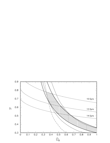
Figure 1: The constraints plotted in the $\Omega_{0}$–$h$ plane, assuming baryon density as given by standard nucleosynthesis. All models are normalized to the COBE data as given by GRSB, and the constraints shown are all at 95 per cent confidence. The solid lines are limits on the shape parameter. The dashed lines are limits from the cluster abundance. The dot-dashed line is the lower limit from POTENT (since it comes from confidence intervals, formally it is $97.5$ per cent as a lower limit, the upper limit not being shown here). Finally, the labelled dotted lines are contours of constant age as indicated. The shaded region shows the parameter space not excluded at greater than 95 per cent on any single piece of data.

Figure 2: A chi-squared plot in the $\Omega_{0}$–$h$ plane. This plot includes all the data that we have discussed. In contrast to Fig. 1, the COBE data are included with their uncertainty error bar. The main compromise is the condensation of the Peacock & Dodds data set down to just the shape parameter; otherwise its slightly low chi-squared is excessively generous to the other data as discussed. The inner contour corresponds to 68 per cent confidence, the outer one to 95 per cent confidence. Age contours are also shown, but are not included in the chi-squared. The chi-squared plot supports the picture formed from Fig. 1, with the drawback of concealing which data are primarily responsible for the trends.

At redshift $z=4$, the contribution of the damped Lyman alpha systems to the density in baryons is estimated as

$$\Omega_{{\rm DLAS}}=(0.0011\pm 0.0002)\,h^{-1}\,\sqrt{\frac{1+\Omega_{0}z}{1+z}}\,,$$ (31)

where we have conservatively assumed that all the gas in these systems is in the neutral state. Remembering that we are taking the dark matter to be cold, it is a reasonable hypothesis that the total density of these systems is bigger by a factor $\Omega_{0}/\Omega_{{\rm B}}$, where $\Omega_{{\rm B}}=0.0125h^{-2}$ is the average baryon density given by nucleosynthesis. If $M$ is the typical mass of the systems, this implies that the fraction $f(>M,z)$ of the total mass that resides in bound objects of mass at least $M$ at redshift $z=4.0$ satisfies

$$f(>M,z=4.0)>(0.088\pm 0.024)\,h\,\sqrt{\frac{1+\Omega_{0}z}{1+z}}\,,$$ (32)

where a 20 per cent uncertainty in the baryon fraction has been added in quadrature to the observational uncertainty.

Since we want a lower bound on the density perturbation we take the lower end of the error bar. Bearing in mind that there is no evidence that damped Lyman alpha systems at high redshifts are completely collapsed objects, as we only observe their baryonic component which is able to collapse faster through radiative cooling (e.g. Katz et al. 1994), we conservatively assume that these systems are more akin to collapsing protospheroids (see also Lanzetta et al. 1995). In order to reflect this choice we will use $\delta_{{\rm c}}=1.5$ in the Press–Schechter calculation, which some numerical studies (e.g. Monaco 1995) have shown is associated with the time-scale of gravitational collapse of a perturbation along its first two collapsing axes, i.e. ‘filament’ formation. Also, in order to be compatible with lower redshift observations, the collapsing protospheroids have to be massive enough eventually to give rise to rotationally supported discs [Lanzetta et al. 1995]. Therefore we take the minimum mass of damped Lyman alpha systems to be $10^{10}\,h^{-1}\;{{\rm M}}_{\sun}$ [Haehnelt 1995], which corresponds to a circular velocity of about $75\;{\rm km}\,{\rm s}^{-1}$. Although formally the constraint as calculated above is only a 1$\sigma$ lower limit, it is almost unchanged by going to 2$\sigma$.

5 Discussion

We plot the data that we have discussed in two separate ways. The first is direct contouring of the observations in the $\Omega_{0}$–$h$ plane, in Fig. 1. For this figure we have fixed the normalization of the spectrum by the COBE measurement, taking advantage of its small error bar. It turns out that the constraint based on the abundance of damped Lyman alpha systems is very weak (both in the critical density case and for general $\Omega_{0}$) as compared to other constraints, and so for clarity we do not plot it. All other data play some role in constraining the allowed parameters, though the shape parameter and cluster abundance allow very similar regions. We use the age constraint to cut off the region at the very conservative value of 10 Gyr.

The second type of plot, Fig. 2, shows chi-squared contours of the data. The only difference in input data is that we treat the COBE data with their uncertainty, so that at each point in parameter space the chi-squared statistic is that for the optimal normalization. The chi-squared plot has the advantage of producing a simple summary of the constraints, but the drawback that one cannot tell which of the data are predominant in contributing to the constraints.

Most of the recent literature on structure formation models has concentrated attention either on retaining $\Omega_{0}=1$ and making other modifications such as introducing a hot dark matter component, or on reducing $\Omega_{0}$ all the way down to 0.2 or 0.3. We notice that the best fits with the new COBE normalization favour rather higher values, the lowest permitted being about $\Omega_{0}=0.35$. Further, good fits are available for the whole continuum of $\Omega_{0}$ values above this, for a suitable choice of Hubble parameter. Without inputting extra information on the preferred values of $h$, the observational data indicate no particular preference for any value of $\Omega_{0}$.

A variety of recent measurements of the Hubble parameter have favoured higher values (e.g. Schmidt et al. 1994; Freedman et al. 1994). While we feel that the situation has yet to be completely closed, it is interesting to examine the reduction in parameter space implied by choosing $h>0.6$. This still allows a fit to all the data (even allowing an age over 12 Gyr), but such a constraint requires that $\Omega_{0}$ falls in a narrow band between 0.35 and 0.55.

So far in this paper we have assumed that the spectral index of the primordial curvature perturbation is $n=1$. Inflation models typically predict some degree of ‘tilt’ in the spectrum, so that $n$ is not precisely 1. The degree of tilt predicted by inflation is highly model-dependent, ranging from negligible up to a few tenths depending on the inflationary model [Liddle & Lyth 1993]. There is some preference for tilting to $n<1$ but models also exist that act in the opposite direction. There is some reason to believe that tilt is rather more likely in open inflationary models, since special physics is being invoked on scales around the curvature scale. We end with a short discussion of the effect of tilt.

In the case of critical density, there is a strong desire to remove short-scale power from the spectrum, which both tilt and gravitational waves are capable of doing. For low densities, the spectrum has already had its shape altered by the shifting of matter–radiation equality, and so there is less freedom to shift $n$ from the scale-invariant value. In the absence of a definite prediction of tilt from an inflationary model, we shall examine the two cases $n=0.9$ and $n=1.1$. The effect of gravitational waves in an open universe has not been successfully quantified yet and we do not include them here.

Tilting corresponds to taking $\delta_{H}^{2}(\Omega_{0})$ to be scale-dependent, given by

$$\delta_{H}^{2}(k,\Omega_{0})=\delta_{H}^{2}(\Omega_{0})\left(\frac{k}{k_{10}}\right)^{n-1}\,,$$ (33)

where $k_{10}$ is some normalization scale where the normalized spectra at different $n$ are assumed to cross (for a given $\Omega_{0}$). A detailed normalization of tilted open models along the lines of Górski et al. [Górski et al. 1995] has not been provided so we need some improvization to normalize the models. We assume that the tenth microwave anisotropy multipole, which acts as a pivot point for the COBE data, is unchanged by tilt; hence the notation $k_{10}$ which is the effective scale of the tenth multipole. The prefactor $\delta_{H}^{2}(\Omega_{0})$ is the normalization for $n=1$, given by equation (10). We find the scale $k_{10}$ from the ‘window function’ which describes how different scales contribute to the tenth multipole; we take $k_{10}$ to be the scale at which the window function, calculated using only the Sachs–Wolfe effect as in García-Bellido et al. [García-Bellido et al. 1995], peaks. We find that $k_{10}$ is very well fitted by the surprisingly simple relation $k_{10}=6\Omega_{0}a_{0}H_{0}$. With this, we can then use equation (33) in equations (1) and (4). This improvization should work very well until $\Omega_{0}$ becomes smaller than about 0.3.

All other data remain the same, though we now need a more general expression for the shape parameter, which at 95 per cent confidence is [Peacock & Dodds 1994]

$$\Gamma=0.255_{-0.033}^{+0.038}+0.32\left(\frac{1}{n}-1\right)\,.$$ (34)

The results are shown in Fig. 3. Increasing $n$ has the effect of shifting the allowed band to lower $\Omega_{0}$, and decreasing $n$ shifts it to higher $\Omega_{0}$, roughly in accordance with $\Delta\Omega_{0}\simeq-\Delta n/2$. Assuming the range $0.9<n<1.1$, we therefore find that the width of the band in the $\Omega_{0}$–$h$ plane is increased, so that for $h>0.6$ the allowed range is roughly $0.30<\Omega_{0}<0.60$.

In conclusion, we have made a thorough investigation of linear theory constraints on cold dark matter models in genuinely open universes, on the assumption that the spectrum of the primordial curvature perturbation is scale-independent. We have also placed these models in their inflationary cosmology context. The normalization to COBE provided by GRSB allows a much more precise comparison with observations than has been made previously. We have included a treatment of the abundances of both clusters and damped Lyman alpha systems; although these have proved constraining for various types of model such as mixed dark matter models, they are easy to satisfy here. On the whole, the new constraints that we have computed support the allowed parameter space from earlier considerations rather than reduce it. We conclude that there is a substantial parameter space still viable for these models.

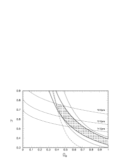
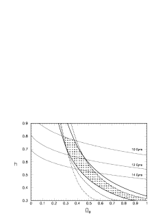
Figure 3: As Fig. 1, but in the case of a tilted spectrum. The top diagram shows $n=0.9$, and the lower shows $n=1.1$.

References

- [Amendola, Baccigalupi & Occhionero 1995] Amendola L., Baccigalupi C., Occhionero F., 1995, Rome preprint, astro-ph/9504097
- [Bardeen 1980] Bardeen J. M., 1980, Phys. Rev. D, 22, 1882
- [Bardeen et al. 1986] Bardeen J. M., Bond J. R., Kaiser N., Szalay A. S., 1986, ApJ, 304, 15
- [Bartelmann & Loeb 1995] Bartelmann M., Loeb A., 1995, CfA preprint, astro-ph/9505078
- [Bennett et al. 1994] Bennett C. L. et al., 1994, ApJ, 436, 423
- [Bernardeau 1994] Bernardeau F., 1994, ApJ, 427, 51
- [Bertschinger & Dekel 1989] Bertschinger E., Dekel A., 1989, ApJ, 336, L5
- [Bruni & Lyth 1994] Bruni M., Lyth D. H., 1994, Phys. Lett., B323, 118
- [Bucher & Turok 1995] Bucher M., Turok N., 1995, Princeton preprint, hep-ph/9503393
- [Bucher et al. 1995] Bucher M., Goldhaber A. S., Turok N., 1995, Phys. Rev. D, 52, 3314
- [Carroll, Press & Turner 1992] Carroll S. M., Press W. H., Turner E. L., 1992, ARA&A, 30, 499
- [Colafrancesco & Vittorio 1994] Colafrancesco S., Vittorio N., 1994, ApJ, 422, 443
- [Coleman & de Luccia 1980] Coleman S., de Luccia F., 1980, Phys. Rev. D, 21, 3305
- [Coles & Ellis 1994] Coles P., Ellis G. F. R., 1994, Nat, 370, 609
- [Copi, Schramm & Turner 1995] Copi C. J., Schramm D. N., Turner M. S., 1995, Science, 267, 192
- [Dekel 1994] Dekel A., 1994, ARA&A, 32, 371
- [Demarque et al. 1991] Demarque P., Deliyannis C. P., Sarajedini A., 1991, in Shanks T., Banday A. J., Ellis R. S., Frenk C. S., Wolfendale A. W., eds, Observational Tests of Cosmological Inflation, Kluwer, Dordrecht, p. 111
- [Efstathiou, Sutherland & Maddox 1990] Efstathiou G., Sutherland W. J., Maddox S. J., 1990, Nat, 348, 705
- [Evrard 1989] Evrard A. E., 1989, ApJ, 341, L71
- [Evrard 1990] Evrard A. E., 1990, ApJ, 363, 349
- [Freedman et al. 1994] Freedman W. L. et al., 1994, Nat, 371, 757
- [García-Bellido et al. 1995] García-Bellido J., Liddle A. R., Lyth D. H., Wands D., 1995, to appear, Phys. Rev. D, astro-ph/9508003
- [Górski et al. 1994] Górski K. M. et al., 1994, ApJ, 430, L89
- [Górski et al. 1995] Górski K. M., Ratra B., Sugiyama N., Banday A. J., 1995, ApJ, 444, L65 [GRSB]
- [Gott 1982] Gott J. R., 1982, Nature, 295, 304
- [Gott & Statler 1984] Gott J. R., Statler T. S., 1984, Phys. Lett., B136, 157
- [Guth & Weinberg 1983] Guth A. H., Weinberg E. J., 1983, Nucl. Phys., B212, 321
- [Haehnelt 1995] Haehnelt M. G., 1995, MNRAS, 273, 249
- [Hanami 1993] Hanami H., 1993, ApJ, 415, 42
- [Henry & Arnaud 1991] Henry J. P., Arnaud K. A., 1991, ApJ, 372, 410
- [Kamionkowski & Spergel 1994] Kamionkowski M., Spergel D. N., 1994, ApJ, 432, 7
- [Kamionkowski et al. 1994] Kamionkowski M., Ratra B., Spergel D. N., Sugiyama N., 1994, ApJ, 434, L1
- [Katz et al. 1994] Katz N., Quinn T., Bertschinger E., Gelb J. M., 1994, MNRAS, 270, L71
- [Kauffmann & Charlot 1994] Kauffmann G., Charlot S., 1994, ApJ, 430, L97
- [Klypin et al. 1995] Klypin A., Borgani S., Holtzman J., Primack J., 1995, ApJ, 444, 1
- [Kofman, Gnedin & Bahcall 1993] Kofman L. A., Gnedin N. Y., Bahcall N. A., 1993, ApJ, 413, 1
- [Lacey & Cole 1993] Lacey C., Cole S., 1993, MNRAS, 262, 627
- [Lacey & Cole 1994] Lacey C., Cole S., 1994, MNRAS, 271, 676
- [Lanzetta et al. 1995] Lanzetta K. M., Wolfe A. M., Turnshek D. A., 1995, ApJ, 440, 435
- [Liddle & Lyth 1993] Liddle A. R., Lyth D. H., 1993, Phys. Rep., 231, 1
- [Liddle & Lyth 1995] Liddle A. R., Lyth D. H., 1995, MNRAS, 273, 1177
- [Lilje 1992] Lilje P. B., 1992, ApJ, 386, L33
- [Linde 1995] Linde A., 1995, Phys. Lett., B351, 99
- [Linde & Mezhlumian 1995] Linde A., Mezhlumian A., 1995, Stanford preprint, astro-ph/9506017
- [Lyth & Stewart 1990a] Lyth D. H., Stewart E. D., 1990a, Phys. Lett., B252, 336
- [Lyth & Stewart 1990b] Lyth D. H., Stewart E. D., 1990b, ApJ, 361, 343
- [Lyth & Woszczyna 1995] Lyth D. H., Woszczyna A., 1995, Phys. Rev. D, 52, 3338
- [Ma & Bertschinger 1994] Ma C.-P., Bertschinger E., 1994, ApJ, 434, L5
- [Metzler & Evrard 1994] Metzler C. A., Evrard A. E., 1994, ApJ, 437, 564
- [Mo & Miralda-Escudé 1994] Mo H. J., Miralda-Escudé J., 1994, ApJ, 430, L25
- [Monaco 1995] Monaco P., 1995, ApJ, 447, 23
- [Navarro et al. 1995] Navarro J. F., Frenk C. S., White S. D. M., 1995, MNRAS, 275, 720
- [Peacock & Dodds 1994] Peacock J. A., Dodds S. J., 1994, MNRAS, 267, 1020
- [Press & Schechter 1974] Press W. H., Schechter P., 1974, ApJ, 187, 452
- [Primack 1995] Primack J. R., 1995, Santa Cruz preprint, astro-ph/9503020
- [Ratra & Peebles 1994] Ratra B., Peebles P. J. E., 1994, ApJ, 432, L5
- [Ratra & Peebles 1995] Ratra B., Peebles P. J. E., 1995, Phys. Rev. D, 52, 1837
- [Sasaki et al. 1993a] Sasaki M., Tanaka T., Yamamoto K., Yokoyama J., 1993a, Phys. Lett., B317, 510
- [Sasaki et al. 1993b] Sasaki M., Tanaka T., Yamamoto K., Yokoyama J., 1993b, Prog. Theor. Phys., 90, 1019
- [Sasaki et al. 1995] Sasaki M., Tanaka T., Yamamoto K., 1995, Phys. Rev. D, 51, 2979
- [Sasaki 1994] Sasaki S., 1994, PASJ, 46, 427
- [Schmidt et al. 1994] Schmidt B. P., Kirschner R. P., Eastman R. G., Phillips M. M., Suntzeff N. B., Hamuy M., Maza J., Avilés R., 1994, ApJ, 432, 42
- [Smoot et al. 1992] Smoot G. F. et al., 1992, ApJ, 396, L1
- [Stockton et al. 1995] Stockton A., Kellogg M., Ridgway S. E., 1995, ApJ, 443, L69
- [Storrie-Lombardi et al. 1995] Storrie-Lombardi L. J., McMahon R. G., Irwin M. J., Hazard C., 1995, Cambridge preprint, astro-ph/9503089
- [Sugiyama 1994] Sugiyama N., Berkeley preprint, astro-ph/9412025
- [Sugiyama & Silk 1994] Sugiyama N., Silk J., 1994, Phys. Rev. Lett., 73, 509
- [Tanaka & Sasaki 1994] Tanaka T., Sasaki M., 1994, Phys. Rev. D, 50, 6444
- [Viana & Liddle 1995] Viana P. T. P., Liddle A. R., 1995, Sussex preprint
- [Walker et al. 1991] Walker T., Steigman G., Schramm D. N., Olive K. A., Kang H.-S., 1991, ApJ, 376, 51
- [White & Bunn 1995] White M., Bunn E. F., 1995, ApJ, 450, 477
- [White et al. 1993a] White S. D. M., Efstathiou G., Frenk C. S., 1993a, MNRAS, 262, 1023
- [White et al. 1993b] White S. D. M., Navarro J. F., Evrard A. E., Frenk C. S., 1993b, Nat, 366, 429
- [Wright et al. 1994] Wright E. L. et al., 1994, ApJ, 420, 1
- [Yamamoto & Bunn 1995] Yamamoto K., Bunn E. F., 1995, Berkeley preprint, astro-ph/9508090
- [Yamamoto et al. 1995a] Yamamoto K., Sasaki M., Tanaka T., 1995a, Kyoto preprint, astro-ph/9501109
- [Yamamoto et al. 1995b] Yamamoto K., Tanaka T., Sasaki M., 1995b, Phys. Rev. D, 51, 2968