Filament Statistics: A Quantitative Comparison of Cold + Hot and Cold Dark Matter Cosmologies with CfA1 Data

Abstract

A new class of geometric statistics for analyzing galaxy catalogs is presented. Filament statistics quantify filamentarity and planarity in large scale structure in a manner consistent with catalog visualizations. These statistics are based on sequences of spatial links which follow local high-density structures. From these link sequences we compute the discrete curvature, planarity, and torsion. Filament statistics are applied to CDM and CHDM ($\Omega_{\nu}=0.3$) simulations of Klypin et al.(1995), the CfA1-like sky catalogs of Nolthenius, Klypin and Primack (1994, 1995), and the CfA1 catalog. For 100 Mpc periodic simulation boxes ($H_{0}=50$ km s^-1 Mpc^-1), we find robust discrimination of over 4$\sigma$ (where $\sigma$ represents resampling errors) between CHDM and CDM. The reduced filament statistics show that CfA1 data is intermediate between CHDM and CDM, but more consistent with the CHDM models. Filament statistics provide robust and discriminatory shape statistics with which to test cosmological simulations of various models against present and future redshift survey data.

Key words: large-scale structure of the Universe — dark matter — cosmology: theory — methods: numerical — methods: data analysis

1 Introduction

We introduce filament statistics, a new class of geometric statistics designed to quantify filamentarity and planarity in large-scale structure. We compare cosmological simulations of pure Cold Dark Matter (CDM) models versus Cold plus Hot Dark Matter (CHDM) models in real space, as well as simulated CfA1-like redshift surveys generated from these simulations versus the CfA1 data. Visual comparison of the models (Brodbeck et al.1995; hereafter BHNPK) shows that the CDM galaxy distribution contains larger clusters and less well-defined filamentary and sheet-like structures than CHDM. The filament statistics presented in this paper confirm as well as quantify these results, showing statistically significant and robust discrimination between the models. Filament statistics represent a new and independent class of statistics whose discriminatory power will likely improve further as larger and more complete redshift surveys become available. We present these initial results to demonstrate the viability of the methods.

Filament statistics are related to the alignment statistic, originally proposed by Dekel (1984): For each galaxy, consider two concentric shells; find the moment of inertia ellipsoid axes defined by galaxies within each shell; and calculate the angle difference between the inertia tensor axes. Presumably, where the angle difference in the major axis is small, there is a filamentary structure present, and where the angle difference in the minor axis is small, there is a sheet-like structure present. By randomly sampling the galaxy distribution at different shell radii, one can then gain a measure of the filamentarity and planarity in large-scale structure at various scale lengths. We found that the alignment statistic barely discriminated between CDM and CHDM in real 3D space, and failed to discriminate the models in redshift space.

Our improvement, and the crux of this paper, is to apply generalizations of this statistic in a geometric network construction (see Hellinger et al.1995). Filament statistics represent a basic implementation of this more general class of statistics. Geometric networks generalize topological networks, where the galaxies are vertices of graphs, by considering the configurations of ordered point sets with related statistical geometric properties. The visualizations of BHNPK show marked differences in the number, size, and continuity of filamentary structures in CHDM and CDM. This inspired us to consider the geometric networks generated by mapping the point set of galaxies into another point set by a prescription that sensitively favors contiguous high density regions. The prescription we employ here is designed to respect the discrete geometric and topological properties of the data; that is, we work with the original point sets of data, either in real space or redshift space. We define three simple statistics to compute on these geometric networks which measure filamentarity and planarity.

The next section describes the algorithm and parameter choices for constructing the geometric network used in filament statistics, and defines the individual statistics. The third section outlines the data on which these statistics were calculated. The fourth section presents results and interpretations. The last section describes future work and further applications of filament statistics.

2 Implementation of Filament Statistics

2.1 The Creation of Link Sequences

The basis of the geometrical network construction used in filament statistics is the creation of link sequences which follow local high density regions, as determined by the principal axis of the local moment of inertia tensor. A link sequence is an ordered set of points which can be visualized as joined by “links”, created by the procedure outlined in the flowchart in Figure 1. A link sequence is started from each galaxy in a catalog of galaxies (or if there are too many, a random subset of such galaxies). The moment of inertia tensor is computed using the masses and positions of galaxies within a range $R$ of the given point; for redshift survey data, we weight by luminosity instead of mass. The eigenvectors and eigenvalues of the inertia tensor are found, and from these the principal axis is determined. The new point in the sequence is created at a distance $L$ (the “link length”) away in the direction of the principal axis, and a link is created which joins the old point to the new point. Note that only the first point in a link sequence is a galaxy; the others are simply points within the catalog volume. A new inertia tensor is computed around this new point, and the procedure is repeated until termination. Sequence termination occurs when there are too few nearby galaxies to reasonably identify an axis. By this prescription, each galaxy generates a sequence of links. If a sequence has enough links, then statistics are computed on this link sequence, otherwise the sequence is discarded. The construction of a link sequence is completely defined by choosing the link length $L$, the maximum radius of galaxies to be included in computation of the moment tensor $R$, and the criteria for termination of a sequence.

2.2 Constructing a Dimensionless Statistic

We would like to construct dimensionless parameters which describe the shapes of structures. For that we need to express all scales in units of some typical length scale of the catalog. A natural choice is the mean intergalactic spacing $\bar{d}\equiv(V/N)^{1/3}$, where $V$ is catalog volume and $N$ is number of galaxies in the catalog, since it provides a length scale without any information about shape or clustering; it is also the simplest choice.

We will consider applications in real space as well as magnitude-limited and volume-limited redshift space. Redshift distortion will produce measurable effects on link sequences, and attempts will be made to understand and quantify these effects. Whereas in real space the mapping of a galaxy into a link sequence is completely well-defined, in redshift space this is no longer true — redshift distortion for a given structure depends on the vantage point chosen to observe the structure. Comparison of the properties of the distributions of link sequences in real and redshift space may provide insights useful for constructing corrections for redshift distortions, which in turn might provide methods for correcting other statistics as well. We defer these corrections to subsequent research and for now consider the simplest statistic, which we show is not adversely affected by redshift distortion.

A complication arises in computing $\bar{d}$ in magnitude-limited catalogs, since the sample incompleteness increases with distance from the Milky Way origin, making $\bar{d}$ a function of radius from origin. A local computation of $\bar{d}$ around a given sequence point (i.e., using $\bar{d}=(V/N)^{1/3}$ for a local volume around the given point) will degrade the statistics, since structure identification will be biased towards underdense regions where $\bar{d}$ is large, which is exactly opposite of what is desired. Instead, $\bar{d}$ should be corrected only for the selection function, which depends only on the distance $r$ from the origin. Since $\phi(L)dL$ is the number density of galaxies between luminosity $L$ and $L+dL$, we can obtain $\bar{d}(r)$ for galaxies visible above the magnitude limit as follows:

$$\bar{d}(r)=\left[{\int^{\infty}_{L_{\em lim}(r)}\phi(L)dL}\right]^{-1/3}$$ (1)

where $L_{\em lim}(r)$ is the luminosity of a galaxy with apparent magnitude 14.5 (the CfA1 magnitude limit) at a distance $r$. $\phi(L)$ is assumed to have Schecter form

$$\phi(L)dL=\phi^{\ast}\biggl{(}{L\over L^{\ast}}\biggr{)}^{\alpha}\exp(-L/L^{\ast}){dL\over L^{\ast}}.$$

The Schecter parameters $\phi^{\ast}$, $L^{\ast}$ and $\alpha$ were best-fit to each real and simulated redshift catalog individually; this procedure is described in Nolthenius et al.(1994, 1995; NKP94 and NKP95, respectively). Note that the true distance $r$ is unknown, and is instead estimated assuming no peculiar velocities, i.e. $r\equiv v/H_{0}$ for a galaxy with radial velocity $v$. A few blueshifted galaxies (mostly in Virgo) do end up on the opposite side of the origin, but the statistics turn out to be insensitive to where these few galaxies are placed. ${\bar{d}(r)}$ is computed and used as the local mean intergalactic spacing at each sequence point in the analysis of magnitude-limited catalogs.

2.3 Link Parameters

The first parameter choice we tried was the simplest, with $L=R=\bar{d}$. The virtue of this definition is that we have a parameter-free statistic, in the sense that the parameters are all determined from intrinsic properties of the data set. Unfortunately, statistics derived from constructions with these “natural” parameters did not discriminate between models for reasons that will be clarified below.

For link length $L=\bar{d}$, but range $R$ left as a free parameter, we obtain discriminatory statistics; this choice of $L$ appears to work as well as any other. However, for $R=\bar{d}$, and $L$ a free parameter, we again find little discrimination between models, or even from a Poisson catalog. $R=\bar{d}$ turns out to be too small to identify a local structure, and is dominated by shot noise. A larger $R$ will yield more points per sphere, thereby lowering shot-noise scatter. Since the $R$ parameter controls the scales of structure being measured by the statistics, it is interesting and instructive to look at statistics as a function of $R$, and the results will be presented that way.

An “optimal” $R$ for a given catalog and statistic may be identified by maximizing the discrimination of the given catalog from the Poisson catalog. In section 4.5 we will show that this optimization yields consistent and well-defined $R_{opt}$ values. We shall call the statistics at $R=R_{opt}$ the reduced filament statistics.

2.4 Termination Criteria

There are three parameters which set the termination criteria for a link sequence. $N_{P,min}$ is the minimum number of galaxies required within a sphere of radius $R$ for a sequence to continue; $N_{P,min}$ was set to 5 so that the determination of the principal axis would be statistically meaningful, and so that a sequence would terminate if it was in a sparse region in the catalog. $N_{L,max}$ sets the maximum number of links for a periodic catalog, and is set so that the total length of a sequence cannot exceed the length of the simulation box. In a redshift survey, the sequence terminates if it exceeds the catalog boundary. $N_{L,min}$ sets the minimum number of links for a sequence to be statistically meaningful. This was set to 4 links (the minimum value for computation of all statistics), but can be increased to explore more extended structures. However, since each link is typically fairly large ($\approx$3 Mpc in the simulations considered, and $\approx$15 Mpc in the sparser CfA1 catalog), 4 links is already exploring a reasonably extended scale.

All the termination parameters were varied over fairly wide ranges. $N_{P,min}$ was varied from 4 to 10 with little change in discrimination or robustness; any higher, and the shot noise generated from fewer sequences became significant. The statistics are independent of $N_{L,max}$ as long it is above about 10, below which shot noise from the small number of links becomes significant; it is about 34 in the periodic simulation boxes. Variations in $N_{L,min}$ had some effect on the results for real and simulated redshift catalogs, since for very small values (2 or 3) shot noise increases from low link sampling, while for a high value (above 10), the number of acceptable sequences decreases so that catalog sampling shot noise becomes large. Discrimination was also insensitive to the choice of either a Gaussian, exponential, or top hat window function; we used a top hat for computational efficiency.

Note that the principal axis of the inertia tensor points in two possible directions. From the initial point, the sequence is propagated in both (opposing) directions until termination, and the entire joined sequence is what is used for statistical analysis, as long as the total number of links is at least $N_{L,min}$. Generally, sequences tended to be non-intersecting but in some cases they oscillated between two points. When this is detected, the sequence is terminated.

2.5 Computation of Statistics

We developed three statistics to compute on a link sequence which measure filamentarity or planarity in an easily interpretable way. We call them planarity, curvature, and torsion. These statistics are defined as angle deviations between inertia ellipsoid axes for consecutive points along a link sequence; the exact definitions are as follows:

• Planarity ($\theta_{P}$) is the angle difference between the minor axis of the inertia tensor for two consecutive points. The geometrical interpretation of planarity is as follows: Given that filaments in large-scale structure often occur at intersections of sheet-like structures, the minor axis of the inertia tensor along the filament measures the strength of the embedding sheet perpendicular to the filament; hence a lower planarity angle indicates the presence of a local sheet-like structure.

• Curvature ($\theta_{C}$) is defined as the angle difference between two consecutive links. Equivalently, it is the angle difference between the major axis of the inertia tensor for two consecutive points. A sequence which is following a well-defined filament will have a low angle difference between links; hence a lower curvature angle indicates greater filamentarity.

• Torsion ($\theta_{T}$) is the angle difference between the plane defined by the first two links and the third link. Torsion measures the strength of the embedding sheet parallel to the filament, a lower torsion indicating a stronger planar structure present.

In all cases, a lower value (angle difference) signifies more structure present in the catalog. As an example, consider a set of points distributed randomly throughout a long, thin cylinder. A sequence will track the cylinder, and the angle deviation between each successive link will be very small; hence curvature will show a very low angle deviation. Conversely, planarity and torsion will show large angle deviations since there is no locally preferred plane in a circular cylinder. For a thin sheet, sequences will randomly walk throughout the sheet, yielding a high curvature angle (indicating no filamentary structure), but low planarity and torsion angles (indicating lots of planar structure).

In large-scale structure, filaments are often embedded within sheets, and thus these statistics are expected to be correlated. Nevertheless it is useful to consider each one separately. A key difference between the statistics is that each requires a different number of sequence points to compute. Planarity is the most local statistic, being computed from only 2 link nodes, while curvature requires 3, and torsion requires 4. While planarity and torsion are in the ideal case purely measures of planarity, torsion is more sensitive to the presence of local filamentary structure since it measures angle differences along the sequence rather than perpendicular to the sequence.

For each of those statistics, an average value is found within a single sequence. Then, for all the sequences in that catalog, a median value is found. We will denote the resulting averaged-then-medianed statistic by a bar, as in $\bar{\theta}_{C}$. This final median value is the value of that statistic for the given catalog at the selected value of $R$. Errors analysis is discussed in section 4.

2.6 Visualization and Algorithm Testing

We have attempted to construct an algorithm which will identify and track filaments. We tested the algorithm on artificially generated point sets of lines and planes of varying thickness. The results conformed to qualitative expectations, that lines should show a great deal of filamentarity and little planarity, and vice versa for planes. Also, the median angle deviations increased with thickness, as expected. Visualizations showed that link sequences were tracking the structure as expected.

When we visualized the link sequences which were generated in an actual CHDM simulation, they tended to lie preferentially in regions of structure, but could not often be associated with visually recognizable filaments. They were also scattered throughout the simulation volume. This is because for the simulations we considered (which will be described in the next section), nearly every galaxy that was tried as a sequence starting point yielded a qualifying ($N_{P,min}\geq 4$) sequence. Thus the parameter set we have chosen does not sufficiently restrict the generated sequences to lie directly along the filaments that are detected by eye. By imposing more severe requirements for sequence qualification, one can tune the algorithm to better recognize filamentary patterns. However, this reduces the number of qualifying sequences to a point where statistics are poor, and hence it is not useful for performing statistically significant comparisons. Our conclusion is that this algorithm is not particularly suited for pattern recognition, and is better suited for statistical comparison of overall structural properties of models. The statistics we compute have simple interpretations, and the results for various models are consistent with the BHNPK visualizations; however, this agreement is not necessarily apparent from visualizations of individual link sequences.

Little effort went into developing analytical predictions for expected values of $\bar{\theta}_{C}$, $\bar{\theta}_{P}$, and $\bar{\theta}_{T}$, even in the case of a Poisson catalog. This is due primarily to the fact that the algorithm was successful in the test cases we considered, and thus a complex and time-consuming analytical prediction was deemed to be low priority. Further numerical testing may also be done by superimposing lines or sheets of varying strengths on a Poisson catalog, and determining how effective the algorithm identifies structure. We leave these endeavors to the future, and instead for now concentrate on applications to the comparison of cosmological models.

3 The Simulations and Data

3.1 The Halo Catalogs

The filament statistics were applied to the simulations described in Klypin, Nolthenius & Primack (1995; KNP95), which are 100 Mpc³ particle-mesh simulations on a 512³ force resolution grid. All had $\Omega=1$ and $H_{0}=50$ km s^-1 Mpc^-1 (which will be assumed throughout). A resolution element, or cell, is 195 kpc. The CDM simulations had 256³ particles, while the CHDM simulations had 256³ cold particles and $2\times 256^{3}$ hot particles, giving a cold particle mass of $2.9\times 10^{9}M_{\odot}$ and $4.1\times 10^{9}M_{\odot}$ for CHDM and CDM, respectively. There were two simulations with pure CDM, one with linear bias factor $b=1.0$ (CDM1) and one with $b=1.5$ (CDM1.5), and two CHDM simulations with $10\%$ baryons, $30\%$ in a single neutrino species and the rest cold dark matter.

CDM1 and both CHDM simulations have linear bias factors which are compatible with the COBE DMR results. CHDM₁ and both CDM simulations were started with identical random number sets describing the initial perturbation amplitudes. It was found in NKP94, NKP95 and KNP95 that Set 1 had, by chance, an unusually high power ($\sim\times 2$) on scales comparable to the box size. However, the CfA1 data appears to show similarly unusual power when compared to the larger APM survey data (NKP95, Vogeley et al.1992, Baugh and Efstathiou 1993). CHDM₂ had a power spectrum more typical of a 100 Mpc box. Thus CHDM₁ should be compared to the CDM simulations for discrimination between models, while CHDM₁ can be compared to CHDM₂ to (conservatively) estimate cosmic variance. Note that by using identical random number set initial conditions, cosmic variance is explicitly removed between the CDM1, CDM1.5 and CHDM₁ simulations. Thus comparisons between these simulations reflect only differences in the underlying physics of the models. These four halo catalogs are summarized in Table 1.

Galaxies are identified initially as dark matter halos with ${{\delta\rho}/{\rho}}>30$ in 1-cell resolution elements (corresponding to about 4 cold particles in a cell) which are local maxima in density. Masses were computed in $3\times 3\times 3$ cells surrounding the maximum (using 1-cell masses made no difference in the results), then halos with $M>7\times 10^{11}M_{\odot}$ were broken up to address overmerging (NKP95).

We also tested filament statistics on catalogs in which we identified galaxy halos as cells with ${{\delta\rho}/{\rho}}>80$. These catalogs gave basic results which were quite similar to the halo catalogs described above, with a slight increase in Poisson errors due to fewer numbers of halos. While the ${{\delta\rho}/{\rho}}>30$ catalogs have too many halos to be associated with visible galaxies, these catalogs still serve our purpose of testing whether these statistics can quantify structure and discriminate between models in real space. Comparisons with real data must be done using simulated redshift-space catalogs.

3.2 The Sky Catalogs

NKP94 and NKP95 describe the construction of the CfA1-like sky-projected redshift catalogs from the simulations described in the previous section, and the merged (to match simulation resolution) CfA1 catalog. In order to distinguish these catalogs which are designed to mimic many observational properties of the CfA1 survey from the halo catalogs described above, we call the CfA1-like sky-projected redshift catalogs the sky catalogs. Several items in sky catalog construction which are of relevance to filament statistics are:

(1) Six view points were chosen from within the CHDM₁ and CHDM₂ simulations satisfying the conditions that the local density in redshift space ($V<750$ km s^-1) is within a factor of 1.5 of the merged CfA1 galaxy density, and the closest Virgo-sized cluster is 20 Mpc away. The CDM view points were required to be on the halos nearest to the CHDM₁ view point coordinates, and thus the corresponding sky catalogs, like the halo catalogs, differ only because of their underlying model physics and not cosmic variance.

(2) To create a sky catalog of CfA1 size (12,000 km s^-1, 2.66 steradians), the periodic halo catalogs were stacked, then cut to form the CfA1 survey geometry; hence structures appear typically $\sim 3-4$ times, although distant galaxies are sampled sparsely.

(3) Each sky catalog was cut to CfA1 numbers before fitting a Schecter luminosity function (after monotonically assigning Schecter luminosities to mass). The scatter in Schecter function parameters among the six view points is thus convolved into the statistics.

3.3 The Effect of Halo Breakup

The most massive halos in the simulation should generally have more than one individual galaxy associated with them (Katz and White 1993, Gelb and Bertschinger 1994). These “overmerged” halos were broken up as described in NKP95 (it is the “preferred method” set of catalogs that was used here). Only 0.5% of CHDM halos required breakup, raising the number of halos with ${\delta\rho/\rho}>30$ by $\sim$16%. CDM1.5 and CDM1 catalogs had higher fractions of massive overmerged halos; 1.3% and 1.7% respectively, raising their breakup halo populations by 35% and 56%, respectively. We expect the halo catalog results to be fairly insensitive to breakup since they probe scales $\sim$3 Mpc and up, much greater than the radius over which fragments are distributed, which is typically $\lesssim 1$ Mpc. Indeed we will show this to be the case in section 4.4.

Despite the larger scales investigated, sky catalogs will be more sensitive to breakup. This is because breakup takes a single massive halo and fragments it into many closely-distributed objects, many of which survive the magnitude limit. When normalized to CfA1 number density, the net effect of breakup is to weight the massive halos more strongly, giving the appearance on average of moving galaxy halos into spherical groups (albeit with some “finger of God” elongation). For a dense catalog, overdense regions will be augmented at the expense of underdense regions, but for sparse catalogs like CfA1, only the densest clusters are augmented, at the expense of filamentary and planar structures. Hence it turns out that breakup tends to systematically reduce the amount of filamentary and planar structure measured in sky catalogs.

4 Application of Filament Statistics

4.1 Results for Halo Catalogs

Filament statistics were applied to the above described halo catalogs catalogs after breakup. Figure 2 shows the results for planarity $\bar{\theta}_{P}$, curvature $\bar{\theta}_{C}$, and torsion $\bar{\theta}_{T}$ vs. $R$, where $R$ is in units of $\bar{d}$. The statistics were computed for each $R$ from 1.0 to 2.5 in increments of 0.1, where discrimination levelled off or began falling. To estimate errors in the halo catalogs, each statistic was computed over a random subset of the catalog. The subset was taken to be as many galaxies as necessary to generate 500 link sequences. Even for $R=1.0$, this never required more than 535 galaxies; at high $R$, hardly any galaxies generated sequences which did not meet the $N_{L,min}=4$ criterion. The catalog was then resampled 10 times to obtain an error estimate. Since there are more than 34,000 galaxies in each catalog, the data is not oversampled. At $R=1.0$, there were on average 5–6 links per sequence; this number rose steadily until $R\geq 1.6$, where sequences were was almost always terminated due to the $N_{L,max}={{\rm 100Mpc}/\bar{d}}\approx 34$ criterion. The average number of galaxies within a sphere of radius $R$ around a given sequence point rose from $\sim$10 at $R=1.0$ roughly linearly to $\sim$50 at $R=2.5$.

Figure 2 shows that all three statistics are generally higher for the CDM simulations as compared with the CHDM simulations, indicating that CDM is less filamentary, has fewer sheet-like structures, and has more (spherical) clustering than the CHDM simulations. This is consistent with the BHNPK visualizations. Thus filament statistics do provide quantitative differentiation between structure seen in the halo catalogs.

Note that all the statistics tend to fall with increasing $R$. This reflects the fact that as the ratio of ${R/L}$ increases, the greater overlap between adjacent spherical windows generates stronger correlations between adjacent inertia tensors, thereby reducing the angle deviations between neighboring inertia ellipsoid axes. There is an additional effect that is peculiar to catalogs possessing inherent filamentary structure: Consider a link sequence tracing a path defined by points contained in a “filamentary structure” of radius $R_{cyl}$. As we increase ${R/L}$ we see an increasingly more linear distribution of points in the window, thus lowering the value of ${\bar{\theta}_{C}}\sim\frac{1}{2}\arcsin(R_{cyl}/{R})$. A similar argument holds for planarity and torsion. In reality, the galaxy distribution is much more complex, but the basic result is that sampling large-scale structure gives ${\bar{\theta}_{C}}(R)$, ${\bar{\theta}_{P}(R)}$, and ${\bar{\theta}_{T}(R)}$ falling at rates greater than in the Poisson case.

The large difference between simulations and the Poisson catalogs provides a good indicator of how effectively structure is identified by filament statistics. Link sequences identify and follow structure in a Poisson catalog by detecting chance alignments of halos which masquerade as contiguous structure due to finite numbers of halos in a given window. We call this effect structure aliasing. Structure aliasing is primarily a low-galaxy-density phenomenon, and hence is most significant at low $R$, where all sequences barely exceed $N_{L,min}$, and each window barely has $N_{P,min}$ halos. In this situation the majority of sequences which qualify will be those lying along such rare chance alignment of halos. Increasing $N_{P,min}$ and $N_{L,min}$ reduces structure aliasing, but the corresponding reduction in qualifying sequences increases shot noise significantly. Instead, we simply choose to be careful about our interpretations at low $R$. For instance, for $R\leq 1.3$ the Poisson catalog statistics rise with $R$, indicating that aliased structure is significant here. Structure aliasing occurs in the models as well, but is less apparent because halos are correlated, yielding more halos surrounding a given point than in the Poisson case. Nevertheless the reduced discrimination for $R\leq 1.3$ is an indication that aliased structure is of comparable strength to real structure at these scales.

At low and high $R$ values, filament statistics discriminate between the CDM models with different biases, as shown in Figure 2. At $R\leq 1.3$ CDM1.5 aliases structure more effectively than CDM1 since it is more diffuse (more Poisson-like), while at larger scales ($\gtrsim 7$ Mpc) the enhanced clustering of CDM1.5 (see BHNPK) tends to trap sequences in spherical clumps more effectively than CDM1, giving higher values. Identification of these effects over a $R$ of 1.0–2.5 (roughly 3.0–7.5 Mpc) indicates the high sensitivity of these statistics to the presence of structure.

The two CHDM simulation results are within each other’s error bars on the scales investigated. Hence for these statistics, cosmic variance between CHDM₁ and CHDM₂ may be comparable to resampling errors in the halo catalogs.

As in Hellinger et al.(1995), here we have introduced a set of metastatistics to compare statistics and assess the effectiveness of our analysis. Discrimination between models for a given statistic $\theta$ can be measured by the signal strength $S^{\theta}_{\rm res}$ between catalogs:

$$S^{\theta}_{\rm res}(1,2)={{|\theta_{1}-\theta_{2}|}\over{\sqrt{\sigma_{\theta_{1}}^{2}+\sigma_{\theta_{2}}^{2}}}}$$ (2)

where $\theta_{1}$ and $\theta_{2}$ are values of statistic $\theta$ for catalogs 1 and 2, respectively, and $\sigma_{\theta}$ is the resampling error for that statistic and catalog. The subscript “res” denotes that the units of $S^{\theta}_{\rm res}$ are 1-sigma resampling errors. To compare CHDM to CDM at COBE normalization while minimizing noise due to cosmic variance, we compare CHDM₁ to CDM1. Figure 3(a) shows $S^{\theta}_{\rm res}$(CDM1,CHDM₁) for the halo catalogs for $\theta=\bar{\theta}_{P},\bar{\theta}_{C},\bar{\theta}_{T}$. Planarity shows the highest signal, but at low $R$ this is spurious since planarity is the most local statistic (requiring only two links for computation) and hence is most sensitive to structure aliasing. The planarity signal between CHDM₁ and CDM1 is high at low $R$, but between CHDM₁ and CDM1.5 it is much lower (as seen in Figure 2), indicating that $\bar{\theta}_{P}$ is the least robust of the statistics against structure aliasing. For $R\geq 1.5$, where structure aliasing is unimportant, all statistics show comparable discrimination of $S^{\theta}_{\rm res}$(CDM1,CHDM₁)$\gtrsim 4\sigma$. Thus filament statistics are fairly discriminatory for the halo catalogs. They are also quite robust; their robustness against halo breakup will be formally investigated later.

4.2 The Effect of Redshift Distortion

Redshift distortion is potentially a major concern for filament statistics when applied to the sky catalogs. Naively, one might assume that filament statistics do not discriminate effects due to internal velocities in clusters (“fingers of God”) from genuine linear structures. This is in general not the case, since link sequences contain directional information. Fingers of God are elongated only in the line-of-sight direction r̂ in redshift space, whereas in general a filament in real space will not be aligned with r̂. Since the largest fingers of God occur at the intersection of real filaments, another effect of redshift space distortion is to misguide sequences and increase the angle deviation of a sequence passing through a cluster. The net effect is seen as a decrease in the amount of detected structure in these simulations.

To test the effect of redshift distortion we applied filament statistics to halo catalogs with overdensity ${\delta\rho}/{\rho}>80$ as we scaled the halo peculiar velocities from 0 to a velocity factor $F_{V}=5$ times their actual values. These catalogs were then mock-observed (no magnitude limit) from the origin, including the effect of redshift distortion, at each $F_{V}$. $F_{V}=0$ represents real space, $F_{V}=1$ represents normal redshift space, and $F_{V}$ is increased until fingers of God become large enough to dominate structure identification. Note that $L=\bar{d}\sim 4-5$ Mpc in these catalogs, and we have taken $R=1.5L$. Error bars are obtained in the same way as in the halo catalogs, by taking 500 galaxy random subsamples and resampling 10 times.

Figure 4(a) shows the effect of the transformation from real to redshift space upon filament statistics for the ${\delta\rho}/{\rho}>80$ halo catalogs. At a $F_{V}=1$, we see little change in the discrimination between the models from $F_{V}=0$, perhaps even an increase in discrimination. Even with velocities scaled to 3 times their actual values the models are still well discriminated. At $F_{V}\geq 4$, fingers of God begin to dominate, as evidenced by the flattening of statistical values vs. $F_{V}$, and the increased resampling error. This test was also run on no-breakup versions of the ${\delta\rho}/{\rho}>80$ halo catalogs, and it was found that the interpretations are virtually independent of breakup in both real and redshift space.

This test indicates that fingers of God are not a dominant contributor to the measured structure when applied to halo catalogs with overdensity ${\delta\rho}/{\rho}>80$. The primary effect of redshift distortion is to decrease strength of structure. Trends vs. $F_{V}$ appear not to be highly model-dependent.

To test how density affects redshift distortion, we also ran the velocity scaling test for the ${\delta\rho}/{\rho}>30$ halo catalogs, and to catalogs with an even greater overdensity, ${\delta\rho}/{\rho}>120$. The ${\delta\rho}/{\rho}>30$ halo catalog results confirmed that the primary effect of redshift distortion is to decrease the amount of structure detected; redshift distortion had even less effect on model discrimination than in the ${\delta\rho}/{\rho}>80$ halo catalogs, and little evidence of distortion was seen even out to $F_{V}=5$.

Figure 4(b) shows the more interesting results for the halo catalogs with overdensity ${\delta\rho}/{\rho}>120$. Here, redshift distortion increased resampling errors (thereby degrading the discrimination between models) somewhat even at $F_{V}=2$, and progressively more severely at higher $F_{V}$. This indicates that higher overdensity cuts make redshift distortion a more severe problem. This is expected, since high density regions in general have higher peculiar velocities. Still, at $F_{V}=1$ (i.e., ordinary redshift space) the discrimination is actually increased over real space. This is because the length and abundance of fingers of God reflect clustering properties, which show true differences between models (NKP94, NKP95). The characteristically longer fingers of God in CDM (due to higher halo peculiar velocities) adds extra dispersion in the link directions which adds to the lesser real space filamentarity in CDM. The result is an amplification of the differences between CHDM and CDM for all of the filament statistics we compute. Curvature and torsion are amplified more than planarity because redshift distortion tends to produce more artificial filaments than artificial sheets, and both curvature and torsion measure angle differences along the filament rather than perpendicular to the filament. In sky catalogs, this amplification is more than counteracted by the increase in statistical error due to lower sample size.

4.3 Results For Sky Catalogs

We present results of filament statistics applied to the sky catalogs after halo breakup in Figure 5. Every galaxy in each sky catalog was tried as a possible sequence starting point. For each catalog, at $R=1.0$, around 500 of the $\approx$2360 galaxies typically generated sequences with number of links exceeding $N_{L,min}=4$. This number rose roughly linearly until $R=2.5$, where $\sim$2200 galaxies qualified, on average, in each catalog. There were systematic differences between the catalogs as well, with CHDM₂ showing the largest number of accepted sequences, about $5-10\%$ more than the CDM models. CHDM₁ showed the lowest number, consistently slightly below the CDM models. At $R=1.0$, there were on average about 5 links per sequence; this number rose fairly linearly with $R$, such that at $R=2.5$, there were around 20 links per sequence. The average number of galaxies within a sphere of radius $R$ around a given sequence point rose from 8–10 at $R=1.0$ roughly linearly to 25–30 at $R=2.5$.

The error estimate for each statistic in sky catalogs was determined from sky variance, by computing the statistic at each of six vantage points, and getting an average value and standard deviation for that statistic. Since our box is relatively small, different viewpoints are still seeing many of the same structures, although with differing depth. Sky variance is therefore expected to underestimate true cosmic variance, perhaps significantly in some cases. With current simulations, a better method of estimating cosmic variance is by comparing CHDM₁ and CHDM₂. NKP94, NKP95 and KNP95 estimate the high power in CHDM₁/CDM1/CDM1.5 would be expected $\sim 10\%$ of the time, translating to a $\sim 1.7\sigma$ deviation from norm, while CHDM₂ was found to be quite typical. Thus CHDM₁ vs. CHDM₂ may be taken as a conservative estimate of $1\sigma$ cosmic variance.

Figure 5 shows the results of filament statistics applied to the sky catalogs after halo breakup. CHDM₁ still shows more structure than either CDM, but CDM1 and CDM1.5 are not discriminated. The interesting new feature is that the two different sets of initial conditions are now discriminated, with CHDM₂ values being lower than CHDM₁ at low $R$, and higher than CHDM₁ at high $R$. Statistics on CDM1 and CDM1.5 show a similar behavior to CHDM₁, indicating that the reason for this difference is because the scales are large enough (median $\bar{d}\sim 15$ Mpc) for the anomalously high large-scale power in initial conditions set 1 to become significant. The extra large scale power in set 1, combined with the artificial replication of structure in the construction of the sky catalogs at 100 to $100\sqrt{3}$ Mpc intervals, gives more structure at large scales in set 1 models than in CHDM₂. Simulations with sufficient volume should not suffer from this problem. The CfA1 catalog follows CHDM₂ more closely than the other simulations over $R\approx 1.2-2.0$, where discrimination from the Poisson catalog is best and the statistics are therefore most reliable.

Visualization showed that link sequences were distributed throughout the sky catalog volume, with very few lying in the foreground, $r\lesssim 20$ Mpc. Recall that $\bar{d}(r)$ is small at low $r$, and the Virgo Cluster, being nearby, contributes hardly any sequences even though it gives a large finger of God. At small $R$, sequences tended to be shorter and terminate within the catalog volume, while at large $R$ they tended to terminate once they exceeded the catalog boundary and found no nearby galaxies. Also, at large $R$ the sequences tended to be preferentially radially directed, because the spheres of radius $R$ tended to extend beyond the catalog volume, and hence the entire catalog contributed as a single radial filamentary structure. This was clearly evident for $R\gtrsim 2.0$, indicating that results for these $R$ values are of dubious validity.

In the halo catalog comparisons we estimated Poisson errors for the statistics and left cosmic variance implicit in the comparison of CHDM₁ and CHDM₂; for the sky catalogs we must consider the total cosmic variance which includes variations due to different realizations of the models as well as the choice of view points in redshift space. CHDM₁ shows more structure than CHDM₂ by $\gtrsim 2\sigma$ (where $\sigma$ are sky variance errors) for all $R\geq 1.5$. We interpret this to mean that sky variance is an inadequate estimate of cosmic variance, which is clearly too large to discrimate between CDM and CHDM for these values of $R$. This effectively restricts the discriminatory ranges of $R$ to $R\approx 1.2-1.3$, and suggests that the sensitivity to cosmic variance is approaching the sensitivity to model parameters. Hence we should be increasingly concerned with more closely comparable local environments as well as more realistic models.

Figure 3(b) shows $S^{\theta}_{\rm sv}$(CDM1,CHDM₁) for the sky catalogs, for $\theta=\bar{\theta}_{P},\bar{\theta}_{C},\bar{\theta}_{T}$. This comparison emphasizes the signal strength with respect to sky variance (denoted by subscript “sv”), as we have intentionally reduced cosmic variance by comparing simulations started from the same initial random numbers. Discrimination between CHDM₁ and CDM1 is strongest in curvature and torsion are, while planarity shows a reduced signal. Planarity is weaker because it is not as significantly amplified by redshift distortion as curvature and torsion, as was shown in section 4.2 (see Figure 4(b)). Recall that CDM shows stronger clustering, which leads to greater redshift distortion, which in turn leads to less structure being detected by these statistics. This accentuates the real space differences between CDM and CHDM. Thus filament statistics convolve information from clustering properties of models when applied to CfA1-like catalogs; sensitivity to clustering will reduce in denser surveys.

To test sensitivity to shot noise, filament statistics were applied to full-sky versions of the sky catalogs, which covered 10.384 steradians and contained $\approx 9200$ galaxies (nearly 4 times the CfA1-like sky catalogs). Since the 2.66 sr catalogs and the 10.384 sr catalogs are derived from the same simulation data set, we are still sampling from the same distribution of cluster sizes and shapes. The resulting signal increased by a factor of $\sim 2$ (for $R\geq 1.3$) as expected from sample size statistics. The degradation of the signal from the halo catalogs to the sky catalogs ($S^{\theta}_{\rm sv}\sim 2.5$ for $R>1.6)$ is thus primarily due to sparseness.

The results before breakup are not shown, but as described in section 3.3 the catalogs before breakup show slightly more structure than after breakup. It turns out this effect represents a $\lesssim 1^{\circ}$ increase in each statistic for the sky catalogs, which is comparable to sky variance errors. There is little difference in $S^{\theta}_{\rm sv}$(CDM1,CHDM₁) for no-breakup sky catalogs. Robustness against halo breakup will be formally investigated in the next section.

The statistics were also applied to 80 Mpc volume-limited versions of the CfA1-like sky catalogs, and left typically 400-500 galaxies in each sky catalog. The statistics showed very large shot-noise scatter, and gave no significant discrimination between models. Volume limiting certainly yields more interpretable statistics, but for CfA1 and our similar-size simulation sky catalogs, there are simply too few galaxies.

4.4 Robustness Against Halo Breakup

Galaxy identification represents the single biggest uncertainty in catalog construction, both in halo catalogs and in redshift space. To investigate robustness against halo breakup and halo identification we take the halo catalogs and sky catalogs before and after breakup, find the change in the value of a given statistic for each $R$, and average the difference over all realizations (CDM1, CDM1.5, CHDM₁ and CHDM₂). Formally, we define the galaxy identification uncertainty factor

$$F_{\rm id}(\theta)=\left\langle{{|\theta_{\rm bu}-\theta_{\rm nobu}|}\over{\sqrt{\sigma^{2}_{\theta_{\rm bu}}+\sigma^{2}_{\theta_{\rm nobu}}}}}\right\rangle_{{\rm realizations}}$$ (3)

where $\theta$ represents the value of the statistic in question, “bu” and “nobu” refer to breakup and no-breakup catalogs, and $\sigma_{\theta}$ represents the error on that statistic, which are from resampling or sky variance. $F_{\rm id}(\theta)<<1$ indicates a statistic which is robust against galaxy identification and halo breakup.

We then compute the combined signal strength by combining the resampling error (for halo catalogs) or sky variance error (for sky catalogs) in quadrature with galaxy identification uncertainty. For halo catalogs,

$$S^{\theta}_{\rm res+id}(1,2)={{S_{\rm res}^{\theta}(1,2)}\over{\sqrt{1+F_{\rm id}^{2}(\theta)}}}$$ (4)

where definitions are as in equation 2. For sky catalogs, the subscript “res” is replaced by “sv”, since sky variance is the relevant error measure.

For the halo catalogs, we compute $S^{\theta}_{\rm res+id}({\rm CHDM}_{1},{\rm CDM}_{1})$ for each statistic for $R=1.0-2.0$. The results are plotted in Figure 6(a). The plot only goes up to $R=2.0$, not 2.5 as before, since halo breakup is more significant at smaller scales. Curvature and torsion show little degradation of signal as for $R\geq 1.5$ as compared to Figure 3(a), indicating that these statistics are quite robust against halo breakup in the range of $R$ where structure aliasing is unimportant. Planarity is less robust, since it is the most sensitive to structure aliasing. In summary, all statistics show $\gtrsim 4\sigma$ discrimination between models regardless of halo breakup.

For the sky catalogs, the robustness against halo identification is not as compelling, as seen by the significantly lower values of $S^{\theta}_{\rm sv+id}$ shown in Figure 6(b) as compared to $S^{\theta}_{\rm sv}$ shown in Figure 3(b). Now, only $1-2\sigma$ discrimination is seen, and only at specific values of $R$. This is a result of the $\lesssim 1^{\circ}$ increase in each statistic from increased clustering due to breakup, as described in section 4.4. This reflects the seriousness of the overmerging problem for observational catalog comparisons when using these statistics. While we have devised a statistic that is very robust with respect to errors in the locations of galaxies as evidenced by the robustness of the halo catalogs, robustness with respect to the identification of galaxies is a much more pernicious problem for the sky catalogs.

4.5 Reduced Filament Statistics

Reduced filament statistics were defined earlier as the value of each statistic for a given catalog at a value of $R$ where the Poisson catalog had its maximum discrimination from the survey data. This definition is motivated by considering the Poisson catalog as the “noise” level for these statistics, the survey as the “signal”, and identifying $R=R_{opt}$ where the signal-to-noise ratio is maximized.

For the halo catalogs, this definition yields an $R_{opt}$ which is not unique, since the signal-to-noise ratio is very large for all statistics and catalogs for all $R\geq 1.5$. Thus reduced filament statistics yield no more information regarding model discrimination than $S^{\theta}_{\rm res}$ for the halo catalogs.

For the sky catalogs, the results are more interesting. The signal-to-noise ratio hits a maximum for all statistics at $R\approx 1.3$, and falls rapidly for smaller or larger $R$ values, suggesting $R_{opt}=1.3$. The optimization occurs because at smaller scales the statistics are dominated by structure aliasing, and at larger scales the sampling windows for inertia tensor computation will more often extend outside the catalog volume, thereby confusing the axis determination and increasing noise. The values of $\bar{\theta}_{P}$, $\bar{\theta}_{C}$, and $\bar{\theta}_{T}$ applied to the sky catalogs at $R_{opt}=1.3$ are shown in Table 2. Also shown is the deviation from the merged CfA1 catalog in units of the error for that statistic, $\Delta_{\theta}={{(\bar{\theta}-\bar{\theta}_{\rm CfA1})}/{\sigma_{\theta}}}$.

From Table 2 it is clear that the simulation which agrees best with CfA1 for all statistics is CHDM₂. The CDM models are ruled out at a $3.1\sigma$ level from $\bar{\theta}_{T}$, and at a $2.4\sigma$ level from $\bar{\theta}_{C}$. There is hope that cosmic variance does not significantly degrade these conclusions, since CHDM₁ and CHDM₂ lie within $1\sigma$ of each other.

Analysis of the no-breakup sky catalogs shows that both CDM1 and CHDM₂ are marginally consistent (i.e. CfA1 lies directly in between), and the other models are ruled out at more than a $2\sigma$ level. Thus reduced filament statistics, like full filament statistics, are not very robust with respect to halo breakup.

5 Conclusions, Future Work, and Connection With Other Statistics

Filament statistics applied to the halo catalogs are sensitive and robust diagnostics of large scale structure that effectively discriminate CDM models from CHDM models. The curvature statistic shows a robust discrimination of $4\sigma$ between CDM and CHDM models. Resampling variance is low, and the result is insensitive to details of galaxy identification. The signal-to-noise ratio between any model and the Poisson catalog is very large for all $R\geq 1.5\bar{d}$, where $R$ is the window radius.

Comparison with CfA1 data is done by creating a sample of CfA1-like redshift catalogs from each of the simulations, and comparing these “sky catalogs” directly to the CfA1 survey. When one views the filament statistics results for sky catalogs over all values of $R$, it is clear that no model tested is completely consistent with CfA1 data. However, both the full and the reduced filament statistics show that, at face value, the CHDM simulation with the more typical initial conditions provides the best fit to CfA1 data. For the reduced filament statistics, conservative estimates are that the CDM model with $b=1.0$ is inconsistent with CfA1 at the $2\sigma$ level, the CDM model with $b=1.5$ is inconsistent at the $3\sigma$ level, and the CHDM model with the less typical initial conditions is barely inconsistent at the $1\sigma$ level. However, these results are not robust with respect to details of galaxy identification.

The success of filament statistics for the halo catalogs indicates that larger, denser redshift surveys coupled with larger simulations will provide a significant increase in the robustness and discriminatory power of these statistics versus real survey data. Denser surveys will lower sensitivity to redshift distortion and lower shot noise in filament statistics. We are looking forward to applying these statistics to other redshift catalogs such as SSRS2, CfA2, and the Sloan Digital Sky Survey, and comparing these data sets to the latest in the rapidly-progressing field of cosmological simulations.

In a broader context, we view this work as illustrative of a methodology for constructing new statistics to analyze spatial data. We described the creation of link sequences, which produces data subsamples extracted and organized to amplify properties of interest in the underlying data set. We emphasize that this is especially important in analyzing nonlinear gravitational structures due to their complex geometries and topologies. A key distinction for filament statistics is that the new point set is guided by the distribution of galaxies, not bound by it (as in Delaunay or Voronoi tessellations, see e.g. van de Weygaert 1991) and thus is more likely to be robust against variations in the galaxy locations and halo breakup, though as we have seen, robustness against galaxy identification is a separate issue. The link sequence approach was conceived of as an intuitive means of simplifying the complex topology of the galaxy point set while preserving the sense of approximate connectivity of its large-scale isodensity surfaces (which the eye might recognize as “filamentarity”).

While we have not developed an analytical prediction for the values of filament statistics, we have tested the algorithm by visualizing the resulting link sequences from artificial configurations of points as well as from simulation data sets. The algorithm does not perform well as a method for identifying individual filaments within a simulation, but by taking large samples of sequences one can obtain statistically significant results which are consistent with BHNPK visualizations of the simulations.

There are many other statistics one can compute on the link sequences when viewed as spatial trajectories; we have only considered their most elementary discrete geometric properties. For example, shape statistical filters (Hellinger et al.1995) can characterize local structures much more effectively than inertia axes. With the rapid progress of computational technology and observational data, filament statistics and other geometric network statistics look to form a new and independent class of statistics against which cosmological models may be tested.

6 Acknowledgements

We acknowledge grants of computer resources by IBM, NCSA, SCIPP, UCO/Lick Observatory, and UCSC Computer Engineering. AK, JRP, and DH acknowledge support from NSF grants and DH also acknowledges support from a DOE grant. RD acknowledges support from the NSF GC3 grant and Lars Hernquist. The simulations were run on the Convex C-3880 at the NCSA, Champaign-Urbana, IL.

Tables

Model Components Bias Init.Cond. No. of Gals. $$\bar{d}$$(Mpc)

CDM1 Set 1 58,121(37,164) 2.58(3.00)

CDM1.5 Set 1 61,690(45,592) 2.53(2.80)

CHDM₁ Set 1 34,000(29,151) 3.09(3.25)

CHDM₂ Set 2 34,554(29,765) 3.07(3.23)

Table 1: Table of halo catalogs ( KNP (95), NKP (95)). The number of galaxies and mean interparticle spacing computed before halo breakup are indicated in parentheses.
^aCOBE-compatible bias.

Catalog       $$\bar{\theta}_{P}$$                                   

CDM1       42.360.99       43.970.56       21.730.41       1.6       2.4       3.1

CDM1.5       42.050.66       44.660.35       22.000.46       1.9       5.8       3.4

CHDM₁       40.250.85       41.460.82       19.560.86       -0.6       -1.4       -1.0

CHDM₂       40.710.43       42.020.70       20.110.43       -0.1       -0.9       -0.8

CfA1       40.77       42.64       20.45       -       -       -

Table 2: Table of reduced filament statistics () for sky catalogs after breakup. For each model, the value of each statistic is shown with sky variance errors, and the deviation from the merged CfA1 catalog is shown in units of that statistic’s error (). Models for which are compatible with CfA1; clearly the CHDM simulations are more compatible.

Captions

Figure 1. Link sequence generation computational flowchart. Here, $R$ is in units of the mean intergalactic spacing $\bar{d}$. For galaxies in redshift space, $\bar{d}$ is a function of the Hubble distance $r=v/H_{0}$, where $v$ is the radial velocity of the galaxy. From the initial galaxy, sequences are propagated in both (opposing) directions along the major axis until termination; if the combined number of links is 4 or more, the entire (combined) sequence “qualifies” for computation; else it is discarded.

Figure 2. Filament statistics (planarity $\bar{\theta}_{P}$, curvature $\bar{\theta}_{C}$, and torsion $\bar{\theta}_{T}$) for the halo catalogs versus $R$ in units of $\bar{d}$, the mean interparticle spacing, for $L=\bar{d}$. This plot shows that filament statistics clearly and consistently discriminate between CDM and CHDM for $R\gtrsim 1.4$. Even the different CDM biases are discriminated at certain $R$ values. Cosmic variance estimated by the difference between CHDM₁ and CHDM₂ is generally smaller than resampling error. The Poisson catalog is well discriminated from any model for $R\geq 1.4$. Note: Values for different models are slightly offset in $R$ to improve visibility.

Figure 3. (a) Signal strengths $S^{\theta}_{\rm res}$(CHDM₁,CDM1), as defined in equation ( 2), for $\bar{\theta}_{P}$, $\bar{\theta}_{C}$, and $\bar{\theta}_{T}$ applied to the halo catalogs. All statistics discriminate fairly well for $R\gtrsim 1.5$. The high $\bar{\theta}_{P}$ signal for $R\lesssim 1.5$ is spurious, owing to structure aliasing at small scales. (b) Signal strengths $S^{\theta}_{\rm sv}$(CHDM₁,CDM1) for the sky catalogs. Curvature and torsion are better discriminators than planarity, and stay around 2$\sigma$ for $R\geq 1.3$.

Figure 4. Filament statistics $\bar{\theta}_{P},\bar{\theta}_{C},\bar{\theta}_{T}$ applied to mock-observed (a) ${\delta\rho/\rho}>80$ and (b) $\delta\rho/\rho>120$ halo catalogs with velocities scaled from velocity factor $F_{V}=0$ (real space) to $F_{V}=5$ times their actual value, with $R=1.5$. Going from real space ($F_{V}=0$) to ordinary redshift space ($F_{V}=1$) decreases the amount of structure detected, but actually increases discrimination between models. In the $\delta\rho/\rho>80$ halo catalogs, only for $F_{V}\gtrsim 4$ do fingers of God significantly degrade the discrimination between models. In $\delta\rho/\rho>120$ halo catalogs, the degradation is significant even at $F_{V}=2$. Thus lower densities increase the contribution due to fingers of God. Note: Values for different models are slightly offset in $F_{V}$ to improve visibility.

Figure 5. Filament statistics for the sky catalogs, versus $R$ in units of ${\bar{d}(r)}$, the mean interparticle spacing. Error bars are larger than in the halo catalog statistics due to sparseness, and Poisson is not as well discriminated from models. CDM shows significantly less planarity, curvature, and torsion than CfA1, while CHDM shows slightly too much. CfA1 does not match with any single catalog over all $R$, but does follow CHDM₂ better than the other models, especially for $1.2\leq R\leq 2.0$. The signal-to-noise ratio between CfA1 and Poisson is highest at $R=1.3$ (note the small Poisson error bar) for all statistics, indicating optimal sensitivity at this $R$. Note: Values for different models are slightly offset in $R$ to improve visibility.

Figure 6. Combined signal strengths as defined in equation 4; compare to Figure 3 to see effect of breakup. (a) $S^{\theta}_{\rm res+ID}$(CHDM₁,CDM1) for the halo catalogs. Comparison with Figure 3(a) shows that breakup causes little degradation for $R\geq 1.5$. (b) $S^{\theta}_{\rm sv+ID}$(CHDM₁,CDM1) for the sky catalogs. The two best statistics, $\bar{\theta}_{C}$ and $\bar{\theta}_{P}$, drop from $\sim 2.5\sigma$ to $\sim 1.5\sigma$ under breakup in the most sensitive range $1.2\leq R\leq 2.0$, most likely due to added variance from breakup fragments’ positional noise.

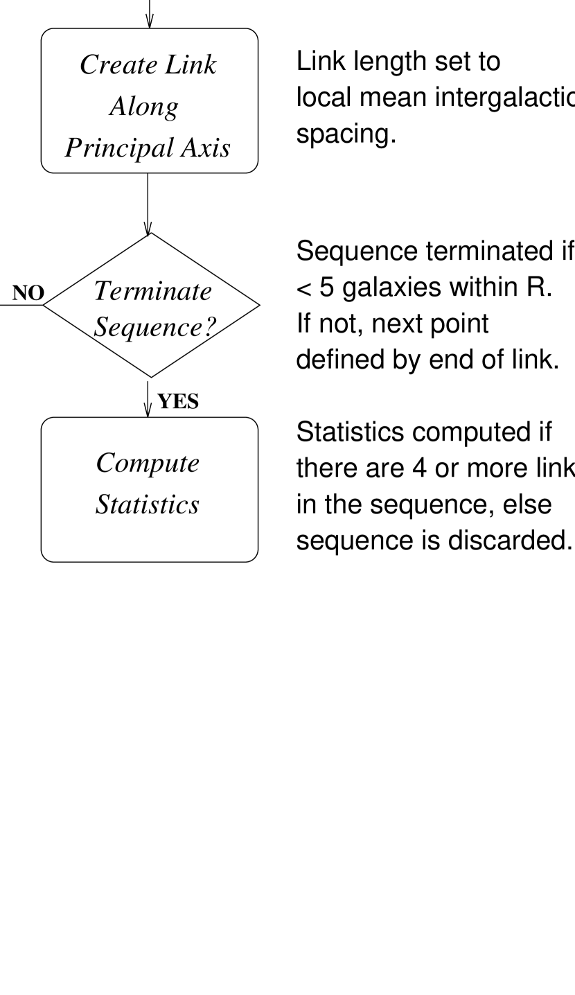
Figure 1:

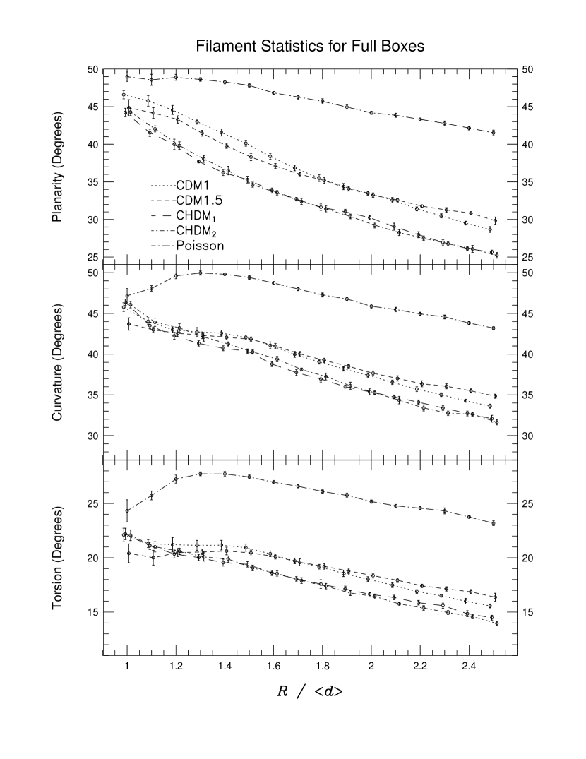
Figure 2:

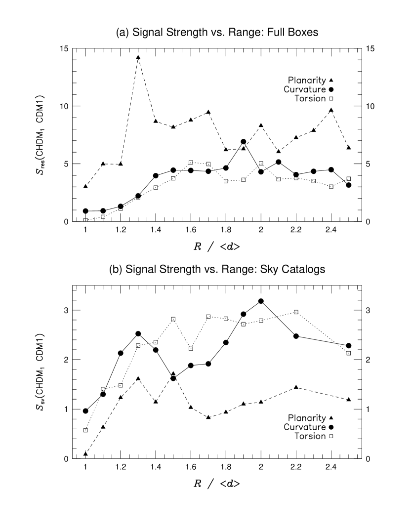
Figure 3:

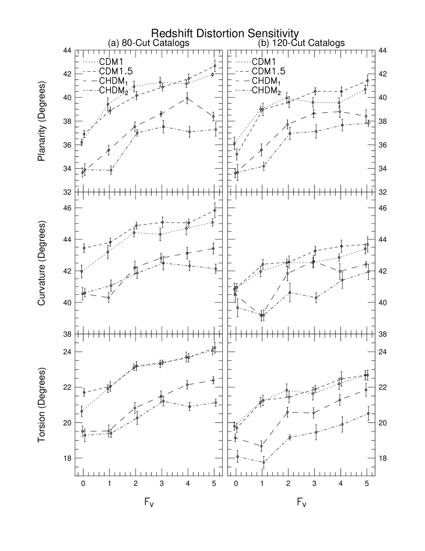
Figure 4:

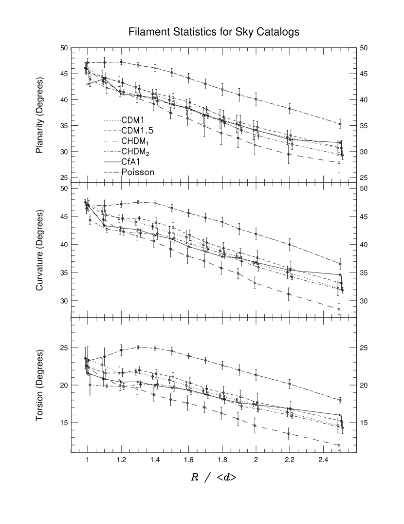
Figure 5:

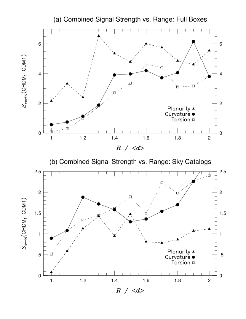
Figure 6:

References

- (1)
- (2) avis, M., Huchra, J., Latham, D.W., & Tonry, J. 1982, ApJ, 253, 423
- (3)
- (4) ekel, A., 1984, in Domokos G., Kovesi-Domokos S., eds, Proc. Johns Hopkins Wkshp. 8, Particles and Gravity. Singapore: World Scientific, p. 206
- (5)
- (6) augh, C.M. & Efstathiou G. 1993, MNRAS, 267, 323
- (7)
- (8) ogeley, M.S., Park, C., Geller, M.J., & Huchra, J.P. 1992, ApJ, 391, L5
- (9)
- (10) rodbeck, D., Hellinger, D., Nolthenius, R., Primack, J.P., & Klypin, A.A. 1995, ApJ submitted [BHNPK]
- (11)
- (12) elb, J., & Bertschinger, E. 1994, ApJ, 436, 467
- (13)
- (14) ellinger, D., Nolthenius, R., Primack, J.P., & Klypin, A.A. 1995, MNRAS to be submitted
- (15)
- (16) atz, N., & White, S. D. M. 1993, ApJ, 412, 455
- (17)
- (18) lypin, A.A., Holtzman, J.A., Primack, J.R., & Regos, E. 1993, ApJ, 416, 1
- KNP (95)
- (20) lypin, A.A., Nolthenius, R., & Primack, J.R. 1995, ApJ, submitted [KNP95]
- NKP (95)
- (22) olthenius, R., Klypin, A.A., & Primack, J.R. 1995, ApJ, in press [NKP95]
- NKP (94)
- (24) olthenius, R., Klypin, A.A., & Primack, J.R. 1994, ApJ, 422, L45 [NKP94]
- vdW (91)
- (26) an de Weygaert, R., 1991 Ph.D. Thesis, Leiden Univ.