Automated classification of IUE low-dispersion spectra

Abstract

Along the life of the IUE project, a large archive with spectral data has been generated, requiring automated classification methods to be analyzed in an objective form. Previous automated classification methods used with IUE spectra were based on multivariate statistics. In this paper, we compare two classification methods that can be directly applied to spectra in the archive: metric distance and artificial neural networks. These methods are used to classify IUE low-dispersion spectra of normal stars with spectral types ranging from O3 to G5. The classification based on artificial neural networks performs better than the metric distance, allowing the determination of the spectral classes with an accuracy of 1.1 spectral subclasses.

1 Introduction

The availability of large spectral archives and the efficiency achieved with modern instrumentation require automated classification methods to improve the classification by visual inspection. These methods are still in exploratory phase; the aims are clear, to devise an objective, repeatable and robust classification scheme providing an estimation of systematic and random errors, and allowing the quantification of spectral resolution and signal to noise ratio on classification errors.

Automated classifiers of stellar spectra can be divided into metric distance algorithms, multivariate statistics and artificial neural networks (hereafter ANN). Metric distance methods were originally proposed by Kurtz and LaSala (Kurtz [1982], [1984], LaSala [1994]) and have been used by Penprase ([1994]) to classify stellar spectra using the digital spectral atlas of Jacoby et al. ([1984]) as template. Multivariate statistical methods are linear algorithms used for exploratory data analysis. These methods have been applied to spectral classification by using Principal Component Analysis (PCA) to reduce the dimension of the problem, followed by Cluster Analysis (CA) to discover groups of objects in the parameter space obtained in the previous step (Murtagh & Heck [1984] and references herein). Stellar classification with ANN is a new approach that has been used by von Hippel et al. ([1994a], [1994b]) to confirm the visual classification of the Michigan Spectral Catalogue on objective prism spectra, determining the temperature classification to better than 1.7 spectral subclasses from B3 to M4. Gulati et al. ([1994]) classify the spectral atlas of Jacoby et al. ([1984]) with an accuracy of 2 spectral subclasses, based on selected spectral features.

The availability of the IUE low-dispersion archive (Wamsteker et al. [1989]) allows the application of pattern recognition methods to explore the ultraviolet domain. The analysis of this archive is especially interesting, due to the homogeneity of the sample. As indicated by Heck ([1987]), it is important to remember at this point that MK spectral classifications defined from the visible range cannot simply be extrapolated to the ultraviolet spectral range. So far, only multivariate statistical methods have been used with IUE spectra. Egret and Heck ([1983]) analyze the relative fluxes at 16 selected wavelengths of O and B stars with PCA. Egret et al. ([1984]) analyze low-resolution spectra using PCA on 93 variables computed as median flux values at certain wavelength bands and selected absorption and emission lines. These analyses indicate a high correlation between the first principal component and the temperature. Heck et al. ([1986]) classify the IUE Low-Dispersion Spectra Reference Atlas (Heck et al. [1984]) of normal stars. Weighted intensities of sixty lines together with an asymmetry coefficient describing the continuum shape are used for the classification. The algorithm consisted of PCA followed by CA to define different groups that confirmed the manual classification of the Atlas. Imadache and Crézé ([1990]) and Imadache ([1992]) extend the sample and generalize the method, using the full spectral range instead of pre-selected spectral features.

The present work has been done within the context of the IUE Final Archive project. The aim is to provide an efficient and objective classification procedure to explore the complete IUE database, based on methods that do not require prior knowledge about the object to be classified. Two methods are compared: a simple metric distance method, and a supervised ANN classifier. The input sample and data preparation steps are described in Sect. 2. The classification method based on metric distance is summarized in Sect. 3. Section 4 explains the classification method using ANN. The results obtained with both methods are described in Sect. 5, and the conclusions are presented in Sect. 6.

2 The sample spectra

The spectra were taken from the IUE Low-Dispersion Reference Atlas of Normal Stars (Heck et al. [1984], hereafter the Atlas), covering the wavelength range from 1150 to 3200 Å. The Atlas contains 229 normal stars distributed from the spectral type O3 to K0. The classification given in the Atlas was carried out following a classical morphological approach (Jaschek & Jaschek [1984]), based on UV criteria alone. The set of 64 standard stars selected in the Atlas, with spectral types from O3 to G5, was used as a template in the metric distance classification and was the training sample in ANN classification. The test set contained 163 spectra, excluding the 64 standard stars and two stars with spectral types G8 and K0, outside the spectral types covered by the training set.

The spectra were obtained by merging together data from the two IUE cameras, sampled at a uniform wavelength step of 2 Å, after processing with the standard calibration pipeline. Although the spectra are good in quality, there are two aspects that seriously hinder the automated classification: interstellar extinction and contamination with geo-coronal Ly-$\alpha$ emission. Some pre-processing was required to eliminate these effects and to normalize the data.

All spectra were corrected for interstellar extinction by using Seaton’s ([1979]) extinction law. Due to the properties of the extinction law at $\lambda_{1}=1600$, $\lambda_{2}=2400$ and $\lambda_{c}=2175$ Å  the color excess $E(B-V)$ was estimated as

$$E(B-V)=1.368\log\left[\frac{225f^{o}_{1}+575f^{o}_{2}}{800f^{o}_{c}}\right]\,.$$ (1)

The observed fluxes $f^{o}_{1}$, $f^{o}_{2}$ and $f^{o}_{c}$ were obtained by filtering the high frequency components in the transformed Fourier space (LaSala and Kurtz [1985]). Figure 1 shows a typical O4 spectrum before and after correction for reddening.

Figure 1: Original (top) and de-reddened (bottom) spectra corresponding to a O4 star. The selected range is indicated by the solid lines in the middle

The region below 1250 Å was excluded from the analysis, to eliminate the geo-coronal Ly-$\alpha$ component, and also the spectral band from 1950 to 2350 Å, because of the low signal to noise ratio in this region. The selected wavelength range is indicated by the solid lines in Fig. 1. The resulting spectra contained $N=744$ flux values, which were normalized to obtain a mean flux value of zero and a sum of the absolute values of the normalized fluxes equal to one.

3 Classification using metric distance

Normalized spectra are considered vectors in $\bbbr^{N}$ and a metric is introduced in the vector space. In this classification scheme the metric distance between the object spectrum and each spectrum in the training set is computed and the spectral class of the star in the training set having the minimum distance is assigned to the object.

Let $f_{ij}=f_{i}(\lambda_{j});\;j=1,\ldots,N$ be the flux of the $i$-th star in the catalogue and $s_{kj}=s_{k}(\lambda_{j});\;j=1,\ldots,N$ be the flux of the $k$-th standard star in the training set, after correction for reddening and normalization. The distance, $d_{ik}$, is defined by

$$d_{ik}^{2}=\frac{1}{N}\sum_{j=1}^{N}(f_{ij}-s_{kj})^{2}\,.$$ (2)

4 Classification using ANN

A supervised classification scheme based on artificial neural networks (ANN) has been used. This technique was originally developed by McCullogh and Pitts ([1943]) and has been generalized with an algorithm for training networks having multiple layers, known as back-propagation (Rumelhart et al. [1986]). In a general form, a neural network represents a function, $F$, that maps a given input set into a selected output set. Assuming that normalized spectra are elements in a $N$-dimensional vector space and spectral classes are defined by $M$-dimensional classification vectors, the network approximates the mapping $F:\bbbr^{N}\rightarrow\bbbr^{M}$, in such a way that a standard star, $\vec{s\/}_{k}$, is associated with the vector $\vec{c\/}_{k}=F(\vec{s\/}_{k})$. The output vector defines the spectral class so that O0 is given by $(1,0,0,\ldots,0)$, O1 is represented by $(0,1,0,\ldots,0)$ and so on. In this form, the network can be regarded as a classifier that maps the input space of normalized fluxes into $1\ of\ M$, i.e., one output unity and all others zero. Such a network, with a squared-error cost function, gives a good estimation of Bayesian probabilities (Richard & Lippmann [1991]), so that for an input spectrum $\vec{f}$, the $i$-th component of the output vector is the probability $P(C_{i}|\vec{f})$ for class $i$ given the input spectrum.

The supervised classifier works in two phases: During a first step, the learning phase, the classifier is trained with the standard stars in the Atlas together with the associated output vectors defining the spectral classes. In a second step, the test sample is presented to the network and spectral types are assigned as defined by the maximum value of the probability distributions estimated by the classifier.

The network architecture consists of an input layer, one or more hidden layers and the output layer. The input layer contains $N$ nodes that accept the individual components of the input vector and distribute them to the nodes in the second layer. Nodes in a layer receive the weighted sum of the output from all the nodes in the previous layer, so that the input of node $j$ is

$$x_{j}=\sum_{i}y_{i}w_{ji}\,,$$ (3)

where $y_{i}$ is the output of node $i$ in the previous layer and $w_{ji}$ is the weight associated to the connection of node $i$ to node $j$. The output of node $j$ is computed using the sigmoid transfer function

$$y_{j}={1\over 1+{\rm e}^{-x_{j}}}\,.$$ (4)

During the training phase, input vectors with normalized fluxes of the standard stars are presented to the network and Eqs. (3) and (4) are applied in a feed-forward mode, until the output layer with $M$ nodes is reached. For each star in the training set, the output vector $\vec{o}$ is compared with the desired classification vector $\vec{c}$, defining the spectral type of the standard star, and the error is evaluated as

$$E={1\over 2}\sum_{j=1}^{M}(o_{j}-c_{j})^{2}\,.$$ (5)

The minimization of the error is achieved during the training phase by changing the connection weights according with the error feedback mechanism, known as back-propagation (Rumelhart et al. [1986]). During this step, connection weights $w_{ji}$ are updated using the rule:

$$\Delta w_{ji}(t)=-\eta{\partial E\over\partial w_{ji}(t)}+\alpha\Delta w_{ji}(t-1)\,,$$ (6)

where $\eta$ is the learning rate, $\alpha$ is the momentum factor to reduce oscillations during the learning process, $t$ is the iteration number and $E$ is the error, given by Eq. (5).

The procedure was repeated for all spectra in the training set in several iterations. The training set was sampled randomly before each iteration, to avoid trends during the learning phase. After each iteration, the average error for all the stars in the training set was computed using Eq. (5), to control the convergency of the procedure. After 2000 iterations there was no substantial improvement in the classification. To prevent excessive corrections during the first iterations, the parameters $\eta$ and $\alpha$ were linearly increased with the iteration number, reaching the operational values of 0.1 and 0.5, respectively, after 100 iterations.

In our study we have used several network configurations, with an input layer consisting of $N=744$ nodes, corresponding to the number of spectral flux values, one or two hidden layers and an output layer having $M=51$ output nodes. A total of six different network topologies were used in the study with 30, 60 and 120 nodes in the hidden layers. In addition, different output distributions were used during the training phase, by convolving the discrete $\delta$ functions representing the class probabilities with gaussian distributions having different standard deviations. The best results were obtained for a standard deviation of $0.7$. Table 1 summarizes the classification statistics for each configuration, the first two columns define the network topology, the third column shows the correlation coefficient, $r$, between the classification obtained with ANN and the manual classification given in the Atlas, and the fourth column is the standard deviation, $\sigma$, of the differences between the two classifications. The network topology $744\times 120\times 120\times 51$ produces the best classification. This network was used in the analysis below. Figure 2 shows the total error, given by Eq. (5), as a function of the number of iterations for the $744\times 120\times 120\times 51$ topology.

Table 1: Network Configurations

Hidden	Hidden
Nodes	Layers	$r$	$\sigma$
120	2	0.988	1.107
60	2	0.983	1.350
30	2	0.946	2.379
120	1	0.984	1.313
60	1	0.986	1.221
30	1	0.982	1.378

Figure 2: Average error as a function of the iteration number for ANN classifier with $744\times 120\times 120\times 51$ topology

Both methods were applied to the test set of 163 stars in the Atlas, excluding the 64 standard stars. In the metric distance method, the class of a test star was determined by the minimum distance given by Eq. (2), there is no way to assess the quality of the classification for a given star. In the classification using ANN, fluxes of a test star are mapped into the classification space, producing an output vector that estimates the Bayesian probabilities for each class. The spectral type is defined by the maximum value of this vector. In addition, the probability distribution provides information on the quality of the classification for each test star.

Figure 3: Results of classification: Metric Distance versus Atlas (top), ANN versus Atlas (middle) and ANN versus Metric Distance (bottom)

Figures 3a and 3b display the correlation between the manual classification given in the Atlas, in horizontal axes, and the classifications obtained with the metric distance and ANN, in vertical axes, respectively. Fig. 3c shows the correlation between metric distance and ANN to demonstrate the consistency of both classification methods. A line of slope unity is also plotted. These figures show a good agreement between automated methods and manual classification, confirming the classification in the Atlas. However, the results obtained with ANN are better than the classification with metric distance.

Table 2: Comparative Performance

	Metric Distance	ANN	ANN vs.
Param.	vs. Catalog	vs. Catalog	Metric Distance
$\sigma$	1.375	1.107	1.144
$r$	0.982	0.988	0.988

Correlation analysis was used to evaluate the performance of the two classification methods. Table 2 summarizes the results, including the standard deviation, $\sigma$, and the correlation coefficient, $r$. The table shows the superior accuracy of the classification obtained with ANN, $\sigma=1.1$, over the metric distance, $\sigma=1.4$. Further analysis of the distribution of the classification errors indicates that 46.6 % of the stars were correctly classified by ANN, i.e., in agreement with the spectral class in the Atlas, while only 35.6 % were correctly assigned using metric distance. Only six stars were classified by ANN with a discrepancy larger than 2 spectral subclasses. Detailed analysis of these objects show a remarkable agreement between both methods. In addition, the classification vectors generated by ANN for these stars have well defined maxima. Figure 4 shows the histogram of the deviations between the classifications produced by ANN and metric distance and the classification given in the Atlas. The superior performance of ANN is evident in these distributions.

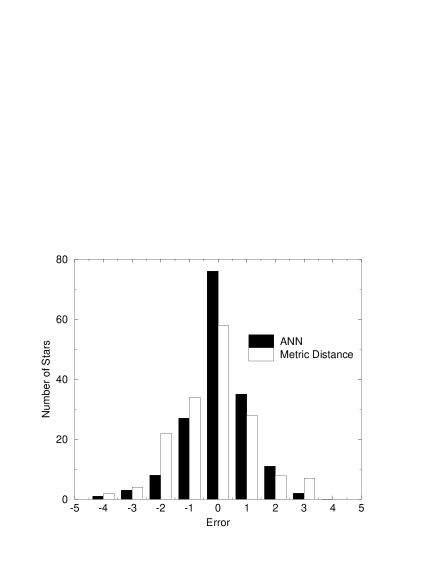
Figure 4: Distribution of classification discrepancies for ANN and Metric Distance versus Atlas

To verify that the ANN classifier gives a good estimation of Bayesian a posteriori probabilities, we have analyzed the output distributions obtained for the complete Atlas. As a first test, the sum of the output distributions should be 1 for each sample star. The estimated mean value for the total set ($K=227$) is

$${1\over K}\sum_{k=1}^{K}\sum_{i=1}^{M}o_{ik}=0.96\pm 0.06\,.$$ (7)

As a second test, the output distribution averaged over the test sample should be equal to the a priori probability distribution in the Atlas, $P(C_{i})$. Figure 5 compares the probability distribution in the Atlas with the averaged output distribution assigned by ANN, estimated as

$${1\over K}\sum_{k=1}^{K}P(C_{i}|\vec{f\/}_{k})={1\over K}\sum_{k=1}^{K}o_{ik}\,.$$ (8)

There is a remarkable agreement between both distributions. The probability values obtained from the Atlas and estimated with ANN are summarized in Table 3 for several ranges of spectral types, confirming that ANN gives an accurate estimation of the Bayesian probabilities. The bias towards hot spectral types, intrinsic to the IUE archive, is also evident in this sample.

Table 3: Probability distributions

Class	Atlas	ANN
O0 - O4	0.048	0.056
O5 - O9	0.141	0.154
B0 - B4	0.322	0.291
B5 - B9	0.185	0.190
A0 - A4	0.132	0.141
A5 - A9	0.066	0.073
F0 - F4	0.075	0.063
F5 - F9	0.022	0.008
G0 - G4	0.004	0.007

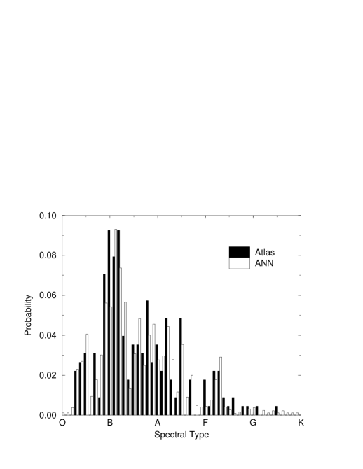
Figure 5: Probability distributions of the spectral classes in the Atlas and estimated by ANN

5 Conclusions

The relative performance of two automated classification methods have been analyzed using IUE low-dispersion spectra of normal stars. The methods do not assume prior knowledge about the spectral types to be classified and the algorithms can be applied directly to the observed flux distributions. The analysis confirms the qualitative results obtained on the same sample, by using multivariate statistics on selected spectral features.

The simple metric distance gives a good classification, but the results produced with the ANN classifier are better. The accuracy obtained with this method is 1.1 spectral subclasses. ANN classifiers have several advantages: they estimate Bayesian probabilities for each spectral type and, in addition, it is possible to identify spectra with uncertain classifications. The method is robust enough to be used in case of spectra with missing information and further improvements can be obtained with IUE spectra by rejecting bad pixels as indicated in the quality flags associated with the spectral values.

This research will be continued to derive physical parameters by using stellar models in connection with observed spectra. Unsupervised ANN classification will be used on the same set.