[

Temperature-Polarization Correlations from Tensor Fluctuations

Abstract

We study the polarization-temperature correlations on the cosmic microwave sky resulting from an initial scale invariant spectrum of tensor (gravity wave) fluctuations, such as those which might arise during inflation. The correlation function has the opposite sign to that for scalar fluctuations on large scales, raising the possibility of a direct determination of whether the microwave anisotropies have a significant tensor component. We briefly discuss the important problem of estimating the expected foreground contamination.

]

COBE’s detection of microwave background temperature anisotropies [1] has excited great interest in theories of cosmic structure formation. Theoretical mechanisms for producing CMB anisotropies include primordial energy density (scalar) and gravitational wave (tensor) fluctuations generated during inflation, or the gravitational fields induced by cosmic defects. These three mechanisms make surprisingly similar predictions for anisotropies on the large angular scales probed by COBE, and further observations are needed in order to discriminate between them. It is clearly of particular value to identify distinctive signals associated with specific physical effects, in order to determine in as direct a manner as possible which mechanisms produced these anisotropies.

The level of temperature fluctuations on smaller scales provides the simplest such test. For example, within inflationary models, the anisotropies due to adiabatic scalar fluctuations generally increase on scales of order the horizon at last scattering (the “Doppler peak”) whereas those due to tensor fluctuations decay away  [2]. However the height of the Doppler peak also depends sensitively on several poorly determined cosmological parameters (for example the Hubble constant and the baryon density), on the ionization history of the universe, and on theoretical model parameters (the details of the inflaton potential [3, 4]). These uncertainties make it difficult to unambiguously determine the size of the tensor contribution [5].

The polarization of the microwave sky could provide invaluable extra information, not far beyond the reach of current experiments. The degree of linear polarization expected from scalar and tensor fluctuations produced during inflation has been calculated  [6, 7, 8, 9, 10], with the result that for a given level of temperature anisotropy tensor perturbations do produce a somewhat larger degree of linear polarization.

Recently we suggested using the temperature-polarization cross correlation $\langle QT\rangle$ as a further test  [11]. Being linear in the polarization, this has some advantages for experiments in which noise in the polarization is limiting, for the latter averages to zero in $\langle QT\rangle$. The $\langle QT\rangle$ correlation also extends to larger angular scales than the auto-correlation function $\langle QQ\rangle$. It thus has particular relevance to experiments with large sky coverage, such as post-COBE satellites now being planned. Here we extend our calculations of $\langle QT\rangle$ to the tensor case, with the result that a striking distinction emerges. On large angular scales the scalar and tensor $\langle QT\rangle$’s have the opposite sign, as a direct result of fundamental differences between scalar and tensor modes. Whether the rather small signal we predict is observable is unclear, depending primarily upon the levels of foreground contamination produced by our galaxy, which as we shall discuss below is still unknown.

We begin with a simplified discussion. To first approximation, recombination may be treated as instantaneous and there is no polarization. The next approximation is to assume that each photon subsequently undergoes a single scattering, after travelling a comoving distance $\lambda$. The photons we now receive from a given direction on the sky emanated from a sphere of radius $\lambda$ surrounding the scattering point (Fig. 1). The Thomson cross section is $\sigma_{T}\propto|$$\boldmath{\epsilon\cdot\epsilon^{\prime}}$$|^{2}$, with $\boldmath{\epsilon}$ and $\boldmath{\epsilon^{\prime}}$ the initial and final photon polarizations. It follows that the photons we measure polarized along the $y$ axis mostly come from above and below the scatterer, and those polarized along the $x$ axis mostly come from the sides of the scatterer.

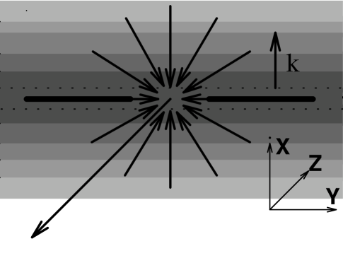
FIG. 1.: A perturbation mode on the surface of last scattering, with the paths of photons which we see coming from a given point on the sky. For scalar perturbations, the direction of linear polarization (heavy lines) is aligned with the temperature troughs. For tensor perturbations the polarization is instead perpendicular.

In Figure 1 a single plane wave perturbation is shown, with its ${\bf k}$ vector perpendicular to the line of sight. For a scalar perturbation, the shading indicates the Newtonian potential $\Phi$, darker indicating more negative $\Phi$. Photons coming from the potential trough are redshifted, so it appears to us as a temperature trough on the sky. Photons coming from above and below the scatterer fall into the potential trough before they scatter, and so are relatively blueshifted. Photons from either side suffer no such shift. So the net linear polarization is aligned parallel to the temperature troughs. By rotating and superposing a set of such modes, one sees that temperature cold spots are surrounded by a radial polarization pattern, hot spots by a tangential pattern. A simple quantitative estimate may be made in the long wavelength limit ($k\lambda\ll 1$), by averaging the Thomson cross section over the sphere of incident photons. The temperature anisotropy is $\delta T/T\approx{1\over 3}\Phi(s)$, with $s$ denoting ‘at the scatterer’. But the polarization depends on the quadrupole moment of $\Phi$ on the sphere - if we expand $\Phi(x,y)$ in a Taylor series, the first terms that contribute involve second derivatives. One finds the fractional linear polarization measured using the $x$, $y$ axes is $Q=-{1\over 20}\lambda^{2}(\partial_{x}^{2}-\partial_{y}^{2})(\delta T/T)(x,y)$, where $T(x,y)$ is the two dimensional temperature field.

Gravitational waves are traceless, transverse excitations of the metric, $g_{\mu\nu}=a^{2}(\eta_{\mu\nu}+h_{\mu\nu})$, where $a$ is the cosmic scale factor. Consider a gravity wave with the same ${\bf k}$ vector and only $h_{zz}=-h_{yy}$ nonzero. The shading in Figure 1 indicates negative $h_{zz}$. The temperature distortion is given by the Sachs-Wolfe integral $-{1\over 2}\int h_{ij,0}n^{i}n^{j}\approx{1\over 2}h_{zz}(s)$, with the dominant contribution coming from the path shared by all photons from the scatterer to us. So again Figure 1 shows a temperature trough on the sky. But for gravity waves initially outside the horizon, if $h_{zz}$ is negative, $\dot{h}_{zz}$ is positive, so the proper distance is being expanded in the $z$ direction, contracted in the $y$ direction. Now we see a fundamental difference with the scalar case. Photons arriving at the scatterer from above and below are unaffected (since the gravity wave is transverse), whereas photons coming from the two sides are blueshifted ($\dot{h}_{yy}$ being negative). The induced polarization pattern is therefore perpendicular to the temperature troughs. Again by rotating and superposing one sees that for gravity waves the temperature cold spots are surrounded by a tangential, hot spots by a radial polarization pattern.

Repeating the ‘single scattering’ calculation explained above, we find $Q\approx{1\over 20}\lambda h_{zz,0}(s).$ A gravity wave mode initially outside the horizon evolves as $h_{zz}\propto 1-Ak^{2}\eta^{2}$, for $k\eta\ll 1$, with $A={1\over 10}$ in the matter era and ${1\over 6}$ in the radiation era. Using this, one finds $Q\approx{1\over 5}A(\partial_{x}^{2}-\partial_{y}^{2})(\delta T/T)(x,y)\lambda\eta_{ls}$, $\eta_{ls}$ being the conformal time at last scattering.

If the temperature autocorrelation function is approximately scale invariant, then $\langle T(\theta,\phi)T(0)\rangle\sim{\rm ln}(1/\theta)$, which is a rough approximation for both scalar and tensor cases for $\theta_{ls}\ll\theta\ll 1$, $\theta_{ls}$ being the angle subtended by the horizon at last scattering. Using the relation between $Q$ and $T$ derived above, one sees that $\langle Q(\theta,\phi)T(0)\rangle\sim{\rm cos}(2\phi)\theta^{-2}$, with coefficients of opposite sign for the scalar and tensor cases. On smaller angular scales, one is sensitive to modes of wavelength smaller than the horizon, which have begun to oscillate by the time of last scattering. In the scalar case oscillations in the photon-baryon fluid density $\delta$ cause the sign of $\langle QT\rangle$ to oscillate, since $T\propto\delta$ and $Q\propto\dot{\delta}$ are out of phase  [11]. Likewise in the tensor case, we have $T\propto h$ and $Q\propto\dot{h}$, so the sign of $\langle QT\rangle$ also reverses. However the redshifting away of gravity waves reduces these oscillations to negligible levels, so that $\langle QT\rangle$ is actually positive for all $\theta\ll 1$. At very small angles, from the ${\rm cos}(2\phi)$ dependence and analyticity it follows that $\langle QT\rangle$ vanishes like $\theta^{2}$.

To calculate $\langle QT\rangle$ accurately we evolve the photon distribution function, ${\bf f}({\bf x},{\bf p},t)$, using the relativistic Boltzmann equation for radiative transfer with a Thomson source term, keeping terms to first order in the perturbation. The distribution function, ${\bf f}$, is a four dimensional vector describing the intensity and polarization degrees of freedom, with components related to the Stokes parameters: $T,Q,U,$ and $V$ [12]. The Boltzmann equation can be rewritten in terms of the perturbed distribution functions, or brightness functions, defined as, $\Delta^{i}\equiv 4\delta f_{i}/\left(T_{0}{{\partial\bar{f}}\over{\partial T_{0}}}\right)$, where $T_{0}$ is the mean CBR temperature, $\bar{f}$ is the unperturbed Planck distribution, $\delta f_{i}$ is its first order perturbation, and $i=T,Q,U$ or $V$.

We evolve the coupled equations by expanding the perturbations in in plane waves. In the case of scalar perturbations, one needs to evolve only two transfer equations, those for the components of ${\bf f}$ corresponding to Stokes’ parameters $T$ and $Q$ [6]. In the tensor case the U component does not vanish but Polnarev[8] has shown with the proper choice of variables,

$$\Delta^{T}(\mu,\phi_{\bf k}) \equiv \alpha(\mu)(1-\mu^{2})\cos(2\phi_{\bf k})$$ (1)

$$\Delta^{Q}(\mu,\phi_{\bf k}) \equiv \beta(\mu)(1+\mu^{2})\cos(2\phi_{\bf k})$$ (2)

$$\Delta^{U}(\mu,\phi_{\bf k}) \equiv \beta(\mu)2\mu\sin(2\phi_{\bf k})$$ (3)

(where $\mu\equiv{\bf\hat{k}}\cdot{\bf\hat{q}}$ and $\phi_{\bf k}$ is the polar angle of ${\bf q}$ about ${\bf k}$) the four Boltzmann equations reduce to just two coupled equations:

$$\dot{\alpha}+ik\mu\alpha = \dot{h}-\sigma_{T}n_{e}a[\alpha+\Psi]$$ (4)

$$\dot{\beta}+ik\mu\beta = -\sigma_{T}n_{e}a[\beta-\Psi]$$ (5)

where,

$$\Psi\equiv\frac{3}{32}\int d\mu^{\prime}[(1+6\mu^{\prime 2}+\mu^{\prime 4})\beta(\mu^{\prime})-(1-\mu^{\prime 2})^{2}\alpha(\mu^{\prime})].$$ (6)

Here, $n_{e}$ is the density of free electrons. These equations are evolved, as in the scalar case[7], by expanding $\alpha$ and $\beta$ in Legendre polynomials (i.e., $\alpha(\mu)=\sum_{l}(2l+1)\alpha_{l}P_{l}(\mu)$), converting them into a hierarchy of ordinary differential equations [2].

Once these variables are evolved to the present epoch, correlation functions are evaluated by summing over ${\bf k}$ and possible polarizations. One finds that the temperature-polarization cross correlation function is,

$$\langle Q({\bf\hat{q}})T({\bf e_{z}})\rangle=\frac{\cos 2\phi}{32\pi^{2}}\int k^{2}dk\sum_{l,l^{\prime}}(2l+1)(2l^{\prime}+1)$$ (8)

$$\hskip 20.0pt\times\biggl{[}{(l^{\prime}-2)!\over(l^{\prime}+2)!}[\alpha_{l^{\prime}}B_{l}\cos^{2}\theta-A_{l^{\prime}}B_{l}]a_{ll^{\prime}}P^{2}_{l^{\prime}}(\cos\theta)$$

$$\hskip 40.0pt+\frac{1}{2}\sin^{2}\theta~{}\alpha_{l^{\prime}}B_{l}\bigl{[}\delta_{ll^{\prime}}\frac{2}{2l+1}P_{l^{\prime}}(\cos\theta)$$ (10)

$$\hskip 100.0pt+{(l^{\prime}-4)!\over(l^{\prime}+4)!}~{}\tilde{a}_{ll^{\prime}}P^{4}_{l^{\prime}}(\cos\theta)\bigr{]}\biggr{]},$$

where $(\theta$, $\phi)$ are the usual spherical polar angles of ${\bf\hat{q}}$, and the axes used to define the Stokes parameters are ${\bf e}_{x}$ and ${\bf e}_{y}$. Here, $A(\mu)\equiv\mu^{2}\alpha(\mu)$, $B(\mu)\equiv(1+\mu^{2})\beta(\mu)$ and the constants $a_{ll^{\prime}}$ and $\tilde{a}_{ll^{\prime}}$ are given by $a_{ll^{\prime}}=\int_{-1}^{1}dxP_{l}(x)P_{l^{\prime}}^{2}(x)$, and $\tilde{a}_{ll^{\prime}}=\int_{-1}^{1}dxP_{l}(x)P_{l^{\prime}}^{4}(x)$ which have simple closed form expressions.

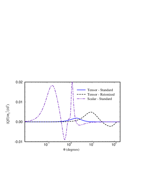
FIG. 2.: $QT$ correlation functions for tensor perturbations in a universe with standard recombination, and in a fully ionized universe, both normalized assuming that the entire COBE detection is due to gravity waves. Shown for comparison is the result for scalar perturbations in a standard scenario [11].

Figure 2 shows $\langle QT\rangle$ for $\phi=0.$ As for $\langle QQ\rangle$, on small scales the tensor $\langle QT\rangle$ is small in comparison to the scalar $\langle QT\rangle$. At large $\theta$ , however, the signals have comparable magnitudes and opposite signs. With substantial early ionization, polarization is greatly enhanced on large angular scales (note also that a geometrical effect causes the tensor $\langle QT\rangle$ to reverse sign for $\theta>30^{o}$.)

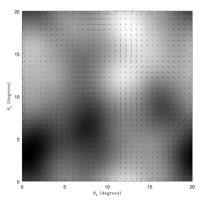
FIG. 3.: $20^{o}\times 20^{o}$ temperature map resulting from tensor perturbations, smoothed on $3^{o}$, with the correlated component of the polarization overlaid.

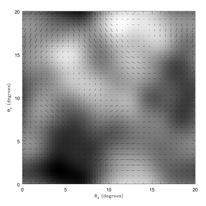
FIG. 4.: As above, but for adiabatic scalar perturbations.

Since the primordial fluctuations are assumed to be described by gaussian statistics, the temperature and polarization are completely described by $\langle QT\rangle$, $\langle TT\rangle$ and $\langle QQ\rangle$, the latter two calculated in [2] and [10] respectively. Using these it is straightforward to construct realizations of the microwave sky [11]. The total polarization $Q$ is composed of parts which are correlated, $Q_{C}({\bf\hat{q}})$, and uncorrelated, $Q_{U}({\bf\hat{q}})$, with the temperature anisotropy. Figure 3 shows the correlated component overlaid on the temperature field. The length of each vector is proportional to $[Q_{C}^{2}(\mbox{\boldmath$\theta$})+U_{C}^{2}(\mbox{\boldmath$\theta$})]^{1\over 2}$ and the orientation is given by $2\phi=\tan^{-1}(U_{C}/Q_{C})$. Hot spots are seen to be associated with radial polarization patterns, while cold spots are surrounded by tangential polarization patterns. For scalar fluctuations on similar scales, however, the opposite is true (Fig. 4).

The power spectrum of $Q$ is compared to that for $Q_{C}$ in Figure 5, showing that in the tensor case the polarization is more strongly correlated with temperature than in the scalar case. The variance $\sigma_{Q_{C}}^{2}$, proportional to the area beneath the curve, comprises more than one third of the variance of the total polarization, $\sigma_{Q}^{2}$. By comparison, for scalar fluctuations the correlated variance is barely a seventh of the total.

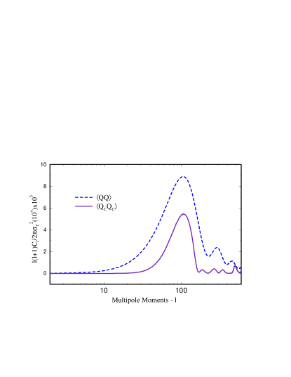
FIG. 5.: The power spectra of the total (dashed line) and temperature-correlated (solid line) polarization in a universe with a standard thermal history normalized to the COBE measurement of the $10^{\circ}$ smoothed temperature variance.

Are these temperature-polarization correlations observable? The main problem is whether sufficient sky coverage can be obtained for a meaningful test. To give ourselves the best possible chance we consider an experiment which covers the whole sky, with very high signal to noise in the temperature measurement. A natural observable is then ${\cal O}={1\over 4\pi}\int d\Omega QQ_{C}$, being the integral of the ‘predicted’ polarization $Q_{C}$ computed from the temperature alone, multiplied by the ‘observed’ polarization $Q$. Since we are only able to make a single measurement, a prediction for ${\cal O}$ is only testable if $S/N\equiv{\cal O}/\sigma_{\cal O}\gg 1$. In Table I we have computed the signal to noise ratios for different beam sizes in a hypothetical full sky experiment. These numbers include only the effects of cosmic variance - instrument noise may be modeled by adding an extra temperature-uncorrelated white-noise component to $Q$ with variance $\sigma_{N}^{2}$. This has the effect of reducing $S/N$ by a factor $(1+\sigma_{N}^{2}/\sigma_{Q}^{2})^{{1\over 2}}$, which may be computed from the values for $\sigma_{Q}$ given in the Table.

Model		Standard			Reionized
	$\Theta$	$\sigma_{Q}$	$\sigma_{Q_{C}}$	$S/N$	$\sigma_{Q}$	$\sigma_{Q_{C}}$	$S/N$
Scalar	0∘	5.2	2.0	420	3.1	1.1	26
	.5∘	1.3	.53	91	3.0	1.0	24
	1∘	.59	.26	49	2.9	.91	19
	5∘	.07	.03	10	1.7	.40	6
Tensor	0∘	.46	.28	89	1.2	.76	18
	.5∘	.41	.25	72	1.2	.76	18
	1∘	.35	.21	57	1.2	.75	17
	5∘	.11	.03	6	.94	.58	12

TABLE I.: Total and correlated polarization in different theoretical scenarios for various beam sizes $\Theta$ (FWHM). $\sigma_{Q}$ and $\sigma_{Q_{C}}$ are given in $\mu K$, with the theories normalized to rms temperature fluctuations of $40\mu K$ for $\Theta=10^{o}$.

Apart from the forbidding challenge of building detectors with the $\mu K$ sensitivities required, the biggest question for using this technique to distinguish scalar and tensor perturbations is whether the polarization signal is swamped by foreground contamination from our galaxy. At frequencies below $\sim 100$ GHz, synchrotron emission is a significant background to CMB experiments, and a typical expectation is linear polarization at the level of $5-10\%$, significantly larger than the effects we are looking for (except perhaps in the fully reionized scenarios). At higher frequencies, dust emission becomes the main background of concern. Here the situation appears much more optimistic, with linear polarization around $1\%$ being typical  [13], although in special regions of very high magnetic field, it can be substantially higher [14]. The frequency dependence of the dust emission may allow one to subtract out dust-associated polarization using multifrequency measurements. In any case we hope the prospect of observing the intriguing signals investigated here will stimulate further study of the likely backgrounds to future full sky polarization measurements.

We thank R. Hills, A. Lasenby, M. Rees and D. Wilkinson for useful conversations. RC thanks R. Davis and P. Steinhardt for collaborating in the initial development of the Boltzmann code. The work of DC was supported by a DOE grant (DOE-EY-76-C-02-3071) while that of RC and NT was partially supported by NSF contract PHY90-21984, and the David and Lucile Packard Foundation.

REFERENCES

- [1] G.F. Smoot et. al., Ap. J. 396, L1 (1992).
- [2] R. Crittenden et. al. Phys. Rev. Lett. 71, 324 (1993).
- [3] R.L. Davis et. al. Phys. Rev. Lett. 69 1856 (1992); L. M. Krauss and M. White, Phys. Rev. Lett. 69, 863 (1992).
- [4] E.J. Copeland et. al., Phys. Rev. D48, 2529 (1993).
- [5] J.R. Bond et.al., Phys. Rev. Lett. 72, 13 (1994); L. Knox and M. S. Turner, FERMILAB-PUB-94-175-A Preprint.
- [6] N. Kaiser, Mon. Not. R. Astr. Soc. 202 1169 (1983).
- [7] J.R. Bond and G. Efstathiou, Ap. J. 285, L45 (1984); Mon. Not. R. Astr. Soc. 226, 655 (1987).
- [8] A.G. Polnarev, Sov. Astr. 29, 607 (1985); R.A Frewin, A.G. Polnarev and P. Coles, MNRAS 266 L21 (1994).
- [9] K.L. Ng and K.W. Ng, Inst. Phys. Academica preprint IP-ASTP-08-93
- [10] R.Crittenden, R. Davis and P.Steinhardt, Ap. J. 417, L13 (1993).
- [11] D. Coulson, R.G. Crittenden and N.G. Turok, Phys. Rev. Lett. 73, 2390 (1994).
- [12] S. Chandrasekhar, Radiative Transfer (Dover, New York, 1960) pp. 1–53.
- [13] R.H. Hildebrand et. al. Ap. J. 417, 565 (1993).
- [14] M. Morris, Ap. J. 399, L63 (1992).