MPI-PhT/94-61

REAL-SPACE COSMIC FIELDS FROM REDSHIFT-SPACE DISTRIBUTIONS:

A GREEN FUNCTION APPROACH

Max Tegmark

Max-Planck-Institut für Physik, Föhringer Ring 6, D-80805 München

max@mppmu.mpg.de

B. C. Bromley

Theoretical Astrophysics, MS B288, Los Alamos National Laboratory,

Los Alamos, NM 87545

bromley@eagle.lanl.gov

1 Introduction

Redshift surveys are testimony to the richness of structure in the universe on large scales (see, for instance, Giovanelli & Haynes 1991). The observed mass distribution in “redshift space”, the space defined by two sky coordinates and a radial recession velocity, depends on both the real-space mass density and the peculiar velocity field, each of which are of great importance in cosmology. The purpose of this paper is to present a new method for evaluating both the density and velocity fields, as well as the peculiar gravitational potential, directly from redshift data.

While quantifying the redshift-space distortions is difficult in general, Kaiser (1987) has solved the problem for large scales ($>10\,{\rm Mpc}$) in the linear regime of gravitational instability theory (Peebles 1993, §5): The effect of linear peculiar flows on the observed redshift-space density field is, loosely speaking, to enhance the amplitude of fluctuation modes along the observer’s line of sight by a factor of

$$\beta={\Omega^{0.6}}/{b}\,,$$ (1)

where the parameter $b$ admits the possibility that there is a linear bias in the fluctuations of luminous matter relative to the total mass distribution. This dependence on $\Omega$ has been exploited to estimate the cosmic mass density from redshift data (Hamilton 1992, 1993; Fisher, Scharf & Lahav 1994; Cole, Fisher & Weinberg 1994; Bromley 1994). For the purposes of removing redshift space distortions, we will assume that $\beta$ is known or that it can be estimated in some self-consistent way from the data.

The problem of reconstructing cosmic fields from redshift data has attracted considerable interest in the last few years. Yahil et al. (1991), Taylor & Rowan-Robinson (1993) and Gramann, Cen & Gott (1994) have implemented iterative algorithms for real-space density and peculiar velocity reconstructions in the linear or quasi-linear regimes. In rough terms, the iterative strategy is to assume that the redshift data approximate the real-space density, calculate the peculiar flows, then correct the density accordingly. The procedure is repeated until the real-space distribution and the velocity field converge to a solution that is consistent with the observed redshifts. A different strategy has been to expand all fields in spherical harmonics, and then estimate each multipole individually (Fisher, Scharf & Lahav 1994; Nusser & Davis 1994).

Here we start with Kaiser’s equation for redshift space distortions and solve for the Green functions that give the real-space density, the peculiar velocity field, and the peculiar gravitational potential. Thus, the reconstruction algorithm simply involves integration over the redshift-space density with a Green function kernel. The method is designed to hold on scales in the linear regime under the assumption that light traces mass or that luminous matter is a linearly biased sample of the total density field. The technique is valid for any survey geometry. In particular, we do not make Kaiser’s “plane-parallel” approximation wherein the redshift survey is assumed to lie in a compact region at a large distance from the observer (see Zaroubi & Hoffman 1994).

The Green function method has distinct advantages over previous techniques: it is a noniterative, linear algorithm applicable to any survey geometry, and the work is done entirely in real space, not in the Fourier domain or with spherical harmonic coefficients. Hence the error bars due to edge effects can be calculated in a straightforward and intuitive way.

This paper is organized as follows. After reviewing Kaiser’s result and establishing some notation in Section 2, we derive the Green function for the peculiar gravitational potential in Section 3, from which the kernels for peculiar velocity and real-space density follow directly. In Section 4, we specialize to the simple case known as the “distant survey approximation”. In Section 5, we discuss how the technique can be applied to real-world situations where one faces nonlinear clustering, shot noise and finite volume. In Section 6, we give a numerical example of density reconstruction from artificial redshift-space data. We conclude by summarizing possible applications of the method for extracting $\Omega$ and constraining the biasing mechanism.

2 The partial differential equation

The first step is to obtain an expression, analogous to a Poisson equation, which relates the real-space peculiar gravitational potential $\phi$ to the density fluctuation field $\delta_{S}$ in redshift space (we denote redshift-space quantities with a subscript-$S$ while subscript-$R$ indicates real space). This was first done by Kaiser (1987), but we give a brief derivation here for completeness.

The fluctuation field is defined in the usual way,

$$\delta=\left[\rho({\bf r})-\overline{\rho}\right]/\overline{\rho}\,,$$ (2)

where $\rho$ is the mass density and $\overline{\rho}$ is its mean. Here, the density fields are associated with luminous matter, and we assume that fluctuations in light are proportional to fluctuations in total mass on the scales of interest. We use time units such that the Hubble constant $H_{0}=1$.

Denoting the radial part of the peculiar velocity field ${\bf v}$ at a real-space position ${\bf r}$ by

$$U({\bf r})\equiv{\bf v}({\bf r})\cdot\widehat{{\bf r}}\,,$$ (3)

and the radial peculiar velocity in the observer’s frame by

$$\Delta U({\bf r})\equiv[{\bf v}({\bf r})-{\bf v}({\bf 0})]\cdot\widehat{{\bf r}}\,,$$ (4)

the apparent position ${\bf s}$ of a galaxy in redshift space is

$${\bf s}({\bf r})\equiv{\bf r}+\Delta U({\bf r})\widehat{{\bf r}}\,.$$ (5)

As long as the perturbations are sufficiently small that this mapping is one-to-one, the overdensities in redshift space and in real space are related by

$$(1+\delta_{R})d^{3}r=(1+\delta_{S})d^{3}s\,.$$ (6)

Evaluating the Jacobian of the mapping (5) yields

$$d^{3}s=\left(1+{\Delta U\over r}\right)^{2}(1+\partial_{r}U)d^{3}r\,,$$ (7)

where $\partial_{r}$ denotes the radial derivative $\partial/\partial r$. Thus, to first order in ${\bf v}$ and $\delta$, and in the absence of selection effects and survey limits, the equation relating the densities in redshift space and in real space is

$$\delta_{S}=\delta_{R}-\partial_{r}U-2{U\over r}+2{{\bf v}(0)\cdot\widehat{{\bf r}}\over r}\,.$$ (8)

We can express the first three terms on the right hand side in terms of the peculiar gravitational potential, $\phi$. The density $\delta_{R}$ and $\phi$ are related through the Poisson equation,

$$\nabla^{2}\phi=A\delta_{R},$$ (9)

where (cf. Peebles 1993, eq. [5.107]) we have introduced the constant

$$A=4\pi G\rho_{0}={3\over 2}\Omega.$$ (10)

In linear theory, the peculiar velocity is simply proportional to the gravitational force field, and is given by (cf. Peebles 1993, eq. [5.117])

$${\bf v}=-{\beta\over A}\nabla\phi.$$ (11)

Thus the velocity terms are

$$\partial_{r}U=-{\beta\over A}\partial_{r}^{2}\phi\,;\ \ \ \ \ {U\over r}=-{\beta\over Ar}\partial_{r}\phi\,.$$ (12)

Substituting this into equation (8) yields what we will refer to as the Kaiser equation,

$$D\phi=A\delta^{\prime}_{S}\,,$$ (13)

where the differential operator $D$ is defined as

$$D\equiv\nabla^{2}+\beta\partial_{r}^{2}+2\beta{1\over r}\partial_{r}\,.$$ (14)

Here we have eliminated the last term in equation (8) by defining $\delta^{\prime}_{S}$ as the redshift space density observed in the cosmic rest frame, the frame relative to which ${\bf v}$ is defined. From the observed dipole anisotropy in the microwave background radiation, we know that the peculiar velocity of our solar system is (Smoot et al. 1992)

$${\bf v}(0)=370\pm 10\,\,{\rm km/s}$$ (15)

in the direction $\alpha=11.2^{h}$, $\delta=-7^{\circ}$. The cosmic variance in this dipole is merely a few km/s, i.e., considerably smaller than the errors quoted above. $\delta^{\prime}_{S}$ can be directly computed from the redshift-space density we observe, $\delta_{S}$, either by using the first order correction derived above,

$$\delta^{\prime}_{S}({\bf r})=\delta_{S}({\bf r})-2{{\bf v}(0)\cdot\widehat{{\bf r}}\over r},$$ (16)

or by simply adjusting the observed redshifts (radial galaxy positions):

$$s^{\prime}=s+{\bf v}(0)\cdot\widehat{{\bf r}}.$$ (17)

In what follows, we will drop the prime and let $\delta_{S}$ denote the corrected field. It should be noted that this distinction is of only marginal importance. The last two terms in equation (8), are usually negligible, and have been dropped by most authors. We leave them in because they preserve the self-adjointness of the operator $D$. It turns out that the approximation of dropping them gives a more complicated solution, not a simpler one.

3 The Green functions

We now solve the Kaiser equation (13). Comparing the differential operator $D$ with the expression for $\nabla^{2}$ in spherical coordinates shows that it is simply the Laplacian with the radial part amplified by a factor $(1+\beta)$. It is self-adjoint for all $\beta$, which means that its eigenfunctions are orthogonal, and that expanding the fields in these functions (spherical Bessel functions of non-integer order) provides a straightforward way of solving the equation. A related formal solution is given by Nusser & Davis (1994), but for a slightly different operator yielding the solution in redshift space, not real space. Here we will instead give a more direct solution, in real space, which renders orthogonal expansions unnecessary.

By the linearity of the problem, we can always write down a formal solution as

$$\phi({\bf r})=A\int{G_{\phi}}({\bf r},{\bf r}^{\prime})\delta_{S}({\bf r}^{\prime})d^{3}r^{\prime}\,,$$ (18)

where the Green function (integral kernel) ${G_{\phi}}$ satisfies

$$(D{G_{\phi}})({\bf r},{\bf r}^{\prime})=\delta^{3}({\bf r}^{\prime}-{\bf r})\,$$ (19)

and the Dirac delta function is distinguished from the fluctuation fields $\delta_{R}$ and $\delta_{S}$ by the absence of a subscript. The constant $A$ in Eq. (18) was inserted to allow us to think of ${G_{\phi}}$ as the operator inverse of $D$. Although ${G_{\phi}}$ is a function of six variables, there are in fact only two quantities upon which the dependence is non-trivial. Since the Kaiser equation is invariant under rotation and rescaling, it is easy to see that we can write

$${G_{\phi}}({\bf r},{\bf r}^{\prime})={g\left(\mu,r/r^{\prime}\right)\over\sqrt{rr^{\prime}}}$$ (20)

for some function $g$, with the angle cosine $\mu\equiv\widehat{{\bf r}}\cdot\widehat{{\bf r}}^{\prime}$. Let us utilize this property by expanding ${G_{\phi}}$ in Legendre polynomials as

$${G_{\phi}}({\bf r},{\bf r}^{\prime})={1\over\sqrt{rr^{\prime}}}\sum_{\l=0}^{\infty}(2\l+1)P_{\l}(\mu)a_{\l}(r/r^{\prime}).$$ (21)

The Kaiser equation implies that the radial functions $a_{\l}(x)$ satisfy

$$a_{\l}^{\prime\prime}+{1\over x}a_{\l}^{\prime}-{1\over x^{2}}\left[{1\over 4}+{l(l+1)\over 1+\beta}\right]a_{\l}={\delta(x-1)\over 4\pi(1+\beta)}.$$ (22)

Requiring $a_{\l}$ to be continuous and imposing the boundary conditions that $a_{\l}(x)$ remain finite both as $x\to 0$ and as $x\to\infty$, this equation has the solution

$$a_{\l}(x)=-{x^{\pm\l}\over 8\pi(1+\beta)\l},$$ (23)

where the exponent is $+\l$ if $x\leq 1$ and $-\l$ if $x\geq 1$, with

$$\l={1\over 2}\sqrt{1+{4\l(\l+1)\over 1+\beta}}\,.$$ (24)

Substitution back into equation (21) gives the solution

$${G_{\phi}}({\bf r},{\bf r}^{\prime})=-{1\over 8\pi(1+\beta)\sqrt{rr^{\prime}}}\sum_{\l=0}^{\infty}\left({2\l+1\over\l}\right)P_{\l}(\mu)\left({r_{<}\over r_{>}}\right)^{\l},$$ (25)

where $r_{<}$ and $r_{>}$ denote the smaller and larger of the numbers $r$ and $r^{\prime}$, respectively. If we let $\beta\to 0$, the Kaiser equation approaches the Poisson equation, $(2\l+1)/\l\to 2$ and equation (25) reduces to the familiar

$${G_{\phi}}({\bf r},{\bf r}^{\prime})=-{1\over 4\pi|{\bf r}^{\prime}-{\bf r}|}.$$ (26)

We now consider the peculiar velocity field ${\bf v}$, which according to equation (11) is proportional to the gradient of the peculiar gravitational potential $\phi$. Rather than computing $\nabla\phi$ numerically, it is convenient to define a Green function ${\bf G_{v}}$ expressly for the velocity field which satisfies

$${\bf v}({\bf r})=\int{\bf G_{v}}({\bf r},{\bf r}^{\prime})\delta_{S}({\bf r}^{\prime})d^{3}r^{\prime}\,,$$ (27)

where, evidently,

$${\bf G_{v}}=\beta\nabla{G_{\phi}}\,.$$ (28)

Taking the gradient of equation (25) with respect to ${\bf r}$ gives

$${\bf G_{v}}({\bf r},{\bf r}^{\prime}) = -{\beta\over 8\pi(1+\beta)r^{\prime 2}}\sum_{\l=0}^{\infty}\left({2\l+1\over\l}\right)\left({r\over r^{\prime}}\right)^{\gamma_{\l}-1}$$

$$\times \left\{\gamma_{\l}P_{\l}(\mu)\widehat{e}_{r}+\l\left[\mu P_{\l}(\mu)-P_{\l-1}(\mu)\right]\widehat{e}_{\theta}\right\},$$

where $\gamma_{\l}\equiv-1/2+l$ if $r<r^{\prime}$ and $\gamma_{\l}\equiv-1/2-l$ if $r>r^{\prime}$. The coordinate $\theta$ refers to a spherical coordinate system with the zenith in the ${\bf r}^{\prime}$-direction, i.e., where $\widehat{{\bf r}}\cdot\widehat{{\bf r}}^{\prime}=\cos\theta$.

For completeness, we finally construct the Green function for the real-space density, ${G_{\delta}}$, such that

$$\delta_{R}({\bf r})=\int{G_{\delta}}({\bf r},{\bf r}^{\prime})\delta_{S}({\bf r}^{\prime})d^{3}r^{\prime}\,.$$ (30)

Since the Poisson equation (9) gives

$${G_{\delta}}=\nabla^{2}{G_{\phi}}\,,$$ (31)

taking the Laplacian of equation (25) yields

$${G_{\delta}}({\bf r},{\bf r}^{\prime}) = {1\over 8\pi(1+\beta)r^{\prime 3}}\sum_{\l=0}^{\infty}\left({2\l+1\over\l}\right)[\gamma(\gamma+1)-\l(\l+1)]P_{\l}(\mu)\left({r\over r^{\prime}}\right)^{\gamma-2}$$ (32)

$$+ \left({3+2\beta\over 3+3\beta}\right)\delta^{3}({\bf r}^{\prime}-{\bf r})\,,$$

where the delta-function term represents the full contribution of ${G_{\delta}}$ at ${\bf r}={\bf r}^{\prime}$. As expected,

$${G_{\delta}}({\bf r},{\bf r}^{\prime})\to\delta^{3}({\bf r}^{\prime}-{\bf r})$$ (33)

in the limit $\beta\to 0$. Contour plots of ${G_{\delta}}$ and the Green function giving the potential, with $\beta=1$, appear in Figure 1. Note that ${G_{\phi}}({\bf r},{\bf r}^{\prime})={G_{\phi}}({\bf r}^{\prime},{\bf r})$, since $D^{-1}$ is self-adjoint, whereas ${\bf G_{v}}$ and ${G_{\delta}}$ lack this symmetry.

4 The distant survey approximation

An interesting limit occurs for a distant-survey (Kaiser 1987, Zaroubi & Hoffman 1994) in which ${\bf r}\approx{\bf r}^{\prime}$ or $|{\bf r}^{\prime}-{\bf r}|\ll r$. For definiteness, let us choose ${\bf r}^{\prime}=\widehat{\bf z}$, the unit vector in the $z$- direction. Then $\partial_{r}\approx\partial_{z}$, the radial part of the Laplacian $\approx\partial_{z}^{2}$, and the Kaiser equation reduces to

$$\left[\partial_{x}^{2}+\partial_{y}^{2}+(1+\beta)\partial_{z}^{2}\right]\phi=A\delta_{s}.$$ (34)

A simple rescaling of the $z$-axis transforms the above expression into the Poisson equation. This fact and the application of the gradient and Laplacian operators to the Green function for the potential immediately give us the three Green functions in the distant-survey limit: defining

$${\bf\Delta r}\equiv{\bf r}-{\bf r}^{\prime}\equiv(\sin\vartheta\cos\phi,\sin\vartheta\sin\phi,\cos\vartheta)\Delta r$$ (35)

and $\mu_{l}\equiv\cos(\vartheta)$, with $\vartheta$ being the angle between ${\bf\Delta r}$ and the line-of-sight (the $z$-axis, parallel to both ${\bf r}$ and ${\bf r}^{\prime}$ in this limit),

$${G_{\phi}}({\bf r},{\bf r}^{\prime})=-{1\over 4\pi{\Delta r}}\left(1+\beta-\beta\mu_{l}^{2}\right)^{-1/2}\,;$$ (36)

$${\bf G_{v}}({\bf r},{\bf r}^{\prime})={1\over 4\pi{\Delta r}^{2}}\left(1+\beta-\beta\mu_{l}^{2}\right)^{-1/2}\left(\widehat{e}_{r}+{\beta\mu_{l}\sqrt{1-\mu_{l}^{2}}\over 1+\beta-\beta\mu_{l}^{2}}\widehat{e}_{\vartheta}\right)\,;$$ (37)

$${G_{\delta}}({\bf r},{\bf r}^{\prime})=\frac{(3+\beta)\mu_{l}^{2}-1-\beta}{4\pi{\Delta r}^{3}\left(1+\beta-\beta\mu_{l}^{2}\right)^{5/2}}+{3+2\beta\over 3+3\beta}\delta^{3}({\bf r}^{\prime}-{\bf r})\,.$$ (38)

Thus ${G_{\delta}}$ vanishes on the cone given by

$$|z^{\prime}-z|=\left({1+\beta\over 2}\right)^{1/2}\sqrt{(x^{\prime}-x)^{2}+(y^{\prime}-y)^{2}},$$ (39)

takes positive values inside this cone and takes negative values outside of it.

5 The real world: nonlinearity, shot noise and finite volume

The above treatment applied to an idealized world were the Kaiser equation was strictly valid, and where we could measure the redshift space density field $\delta_{S}$ accurately throughout all space. Alas, this is not the world in which we live. Below, we discuss the following three sources of error:

1. The Kaiser equation, which is exact to first order, is only accurate when $\delta\ll 1$ and thus breaks down on small scales where nonlinear evolution has become important.

2. Our galaxy surveys do not measure the continuous field $\delta_{R}$ but the discrete galaxy distribution, so our estimates of $\delta_{S}$ are contaminated by Poissonian “shot noise”.

3. Our galaxy surveys sample only a finite volume, which forces us to truncate our volume integrals and accept truncation errors in our reconstructed fields.

There are of course many more potential sources of error, such as nonlinear biasing and flux errors to mention two, but we will restrict our discussion to the three listed problems, which are always present. In what follows, we also limit ourselves to reconstruction of the density field, the analogy for the velocity field and the peculiar gravitational potential being obvious.

5.1 Nonlinear clustering

On small scales, the gravitational evolution has entered into the deeply non-linear regime, where the “fingers-of-God effect” causes virialized clusters to appear elongated along the line of sight. Although some authors have attempted to extend the Kaiser equation into the quasi-linear regime using the Zel’dovich approximation, an exact reconstruction of the real-space density is of course impossible in the deeply non-linear regime. Essentially, this is because the gravitational $n$-body problem exhibits chaotic behavior, rendering the inversion problem numerically ill-posed. We thus follow the same approach as all previous authors, and smooth all our fields ($\delta_{S}$, $\delta_{R}$, etc.):

$$\delta_{S}({\bf r})\mapsto(W\star\delta_{S})({\bf r})=\int W({\bf r}^{\prime}-{\bf r})\delta_{S}({\bf r}^{\prime})d^{3}r^{\prime},$$ (40)

the star denoting convolution. For definiteness, let us choose a Gaussian smoothing kernel

$$W({\bf r})\equiv{1\over(2\pi)^{3/2}r_{s}^{3}}e^{-{1\over 2}(r/r_{s})^{2}},$$ (41)

and choose the smoothing scale $r_{s}$ to be large enough that the resulting fields can be expected to obey linear theory.

5.2 Shot noise

What we measure is of course not the smooth field $\delta_{S}$ but the discrete galaxy density $n({\bf r})=\sum\delta({\bf r}-{\bf r}_{i})$, with a delta function at the location ${\bf r}_{i}$ of each galaxy. We estimate the unsmoothed density by simply $\delta n/{\bar{n}}\equiv(n-{\bar{n}})/{\bar{n}}$, where ${\bar{n}}$, the selection function, specifies the survey geometry by giving the expected density of observed galaxies at each position in space. Our estimate of of the redshift space density $\delta_{S}$ is thus the convolution of $n/{\bar{n}}-1$ with the smoothing kernel $W$. Hence our real-world generalization of equation (30) becomes

$$\delta_{R}^{\prime}({\bf r})\equiv\int_{V}{G_{\delta}}({\bf r},{\bf r}^{\prime})\left(W\star\left[{n\over{\bar{n}}}-1\right]\right)({\bf r}^{\prime}),$$ (42)

where the prime on the left hand side has been added to distinguish the estimate $\delta_{R}^{\prime}$ from the true value $\delta_{R}$. We will return to the issue of how to choose $V$, the volume to integrate over, in the following subsection. Since convolution is associative (simply corresponding to multiplication in Fourier space), equation (42) is equivalent to

$$\delta_{R}^{\prime}({\bf r})=\int_{V}(W\star{G_{\delta}})({\bf r},{\bf r}^{\prime})\left[{n({\bf r}^{\prime})\over{\bar{n}}({\bf r}^{\prime})}-1\right],$$ (43)

i.e., to smoothing the Green function (with respect to ${\bf r}^{\prime}$) instead of the galaxy distribution.

Let us, as is customary, model $n$ as a Poisson process whose intensity (average point density) is $\lambda({\bf r})\equiv{\bar{n}}({\bf r})[1+\delta_{S}({\bf r})]$. We model (the smoothed) $\delta_{S}$ as a random field with $\langle\delta_{S}({\bf r})\rangle=0$ and define its correlation function as

$$\xi_{s}({\bf r},{\bf r}^{\prime})\equiv\langle\delta_{S}({\bf r})\delta_{S}({\bf r}^{\prime})\rangle,$$ (44)

but make no assumptions of it being homogeneous, isotropic or Gaussian. Defining the reconstruction error as

$$\Delta({\bf r})\equiv\delta_{R}^{\prime}({\bf r})-\delta_{R}({\bf r}),$$ (45)

we now proceed to compute the statistical properties of this error. Since a Poisson process satisfies

$$\langle n({\bf r})\rangle = \lambda({\bf r}),$$ (46)

$$\langle n({\bf r})n({\bf r}^{\prime})\rangle = \lambda({\bf r})\lambda({\bf r}^{\prime})+\delta({\bf r}-{\bf r}^{\prime})\lambda({\bf r}),$$ (47)

a straightforward calculation shows that

$$\langle\Delta({\bf r})\rangle = 0,$$ (48)

$$\langle\Delta({\bf r})^{2}\rangle = \sigma_{n}({\bf r})^{2}+\sigma_{t}({\bf r})^{2},$$ (49)

where

$$\sigma_{n}({\bf r})^{2} \equiv \int_{V}{\left[(W\star{G_{\delta}})({\bf r},{\bf r}^{\prime})\right]^{2}\over{\bar{n}}({\bf r}^{\prime})}d^{3}r^{\prime},$$ (50)

$$\sigma_{t}({\bf r})^{2} \equiv =\int_{V\hskip-6.25963pt\backslash}\int_{V\hskip-6.25963pt\backslash}{G_{\delta}}({\bf r},{\bf r}^{\prime}){G_{\delta}}({\bf r},{\bf r}^{\prime\prime})\xi_{S}({\bf r}^{\prime},{\bf r}^{\prime\prime})d^{3}r^{\prime}d^{3}r^{\prime\prime}.$$ (51)

When computing $\sigma_{n}^{2}$, the shot noise error, the integral is to be taken over the volume $V$ (see below). When computing $\sigma_{t}^{2}$, the truncation error, the integrals are to be taken over all space except the volume $V$. Equation (48) simply tells us that our reconstruction is unbiased, in the sense that the expectation value of the error is zero. The remainder of this subsection is devoted to the shot noise term in Equation (49).

Although the shot noise error $\sigma_{n}$ is easily computed numerically using equation (50), it is instructive to make a crude estimate of it. First, let us assume that ${\bar{n}}({\bf r})$ is constant, so that we can factor it out of the integral in equation (50). Second, let us make the distant survey approximation for ${G_{\delta}}$ (this is a good approximation if ${\bf r}$ is more than a few smoothing lengths away from us, as it is easy to show that the smoothed Green function $W\star G$ falls off rapidly, at least as fast as $r^{-3}$, for $|{\bf r}-{\bf r}^{\prime}|\gg r_{s}$, so that the main contribution to the integral comes from within a few smoothing lengths of ${\bf r}$). Third, let us overestimate $\sigma_{n}^{2}$ slightly by extending the integration to all space (this makes only a minor difference, as we will find it optimal to integrate considerably beyond the smoothing scale anyway). Now we can apply Parseval’s theorem and the convolution theorem to the remaining integral, and obtain

$$\sigma_{n}^{2}\approx{1\over(2\pi)^{3}{\bar{n}}}\int|\widehat{{G_{\delta}}}({\bf k})|^{2}|\widehat{W}({\bf k})|^{2}d^{3}k,$$ (52)

where hats denote Fourier transforms. From equation (34), we immediately recover Kaiser’s familiar result

$$\widehat{{G_{\delta}}}({\bf k})\approx\left[1+\beta{\left(k_{z}\over k\right)^{2}}\right]^{-1},$$ (53)

so substituting this into equation (52), we obtain the estimate

$$\sigma_{n}^{2}\approx{1\over(2\pi)^{3}{\bar{n}}}\int{e^{-(r_{s}k)^{2}}k^{2}\sin\theta\over\left[1+\beta\cos^{2}\theta\right]^{2}}\>dk\,d\theta\,d\phi=\left({\arctan\sqrt{\beta}\over 8\pi^{3/2}\sqrt{\beta}}\right)\left({1\over{\bar{n}}r_{s}^{3}}\right).$$ (54)

Defining the effective smoothing volume

$$V_{s}\equiv\left({8\pi^{3/2}\sqrt{\beta}\over\arctan\sqrt{\beta}}\right)r_{s}^{3},$$ (55)

we can conclude this section with the familiar-looking shot noise formula

$$\sigma_{n}^{2}\approx{1\over{\bar{n}}V_{s}}.$$ (56)

In other words, the crucial quantity is the expected number of galaxies in a smoothing volume.

5.3 Finite volume

Although the truncation error $\sigma_{t}$ is straightforward to compute numerically given any prescribed volume $V$, either by evaluating the integral in equation (51) or by making reconstructions from Monte Carlo galaxy catalogs, we now make a very crude estimate $\sigma_{t}$ to obtain a qualitative understanding of how to best choose $V$ and the smoothing scale. Although the unsmoothed fields $\delta_{R}$ and $\delta_{S}$ have ample structure on very small scales, the corresponding smoothed fields are virtually featureless on scales $r\ll r_{s}$. Hence the correlation $\xi_{s}$ is almost perfect for $|{\bf r}^{\prime}-{\bf r}|\ll r_{s}$, and typically falls off like some power law for $|{\bf r}^{\prime}-{\bf r}|\gg r_{s}$. Thus let us make the crude approximation

$$\xi_{s}({\bf r},{\bf r}^{\prime})\approx\cases{\sigma^{2}&for $|{\bf r}^{\prime}-{\bf r}|\ll r_{s},$\cr 0&for $|{\bf r}^{\prime}-{\bf r}|\gg r_{s}$,}$$ (57)

for some constant $\sigma$ which is the r.m.s. fluctuation in a smoothing volume. The only non-negligible contributions to the integrals in equation (51) thus arise when $|{\bf r}^{\prime}-{\bf r}|\mathrel{\hbox to0.0pt{\lower 3.0pt\hbox{$\mathchar 536\relax$}\hss}\raise 2.0pt\hbox{$\mathchar 316\relax$}}r_{s}$. This can be interpreted as there being a large number of independent volumes in which the field is coherent, and that the total variance $\sigma_{t}^{2}$ is simply a sum of the variance arising from each coherence volume that we do not look at, i.e., that falls outside of $V$. Assuming that $V$ is large relative to the smoothing scale, replacing ${G_{\delta}}({\bf r},{\bf r}^{\prime\prime})$ by ${G_{\delta}}({\bf r},{\bf r}^{\prime})$ will thus be a good approximation, and equation (51) reduces to simply

$$\sigma_{t}({\bf r})^{2}\approx a\,\sigma^{2}V_{s}\int_{V\hskip-6.25963pt\backslash}{G_{\delta}}({\bf r},{\bf r}^{\prime})^{2}d^{3}r^{\prime},$$ (58)

where $a$ is some constant of order unity. In the distant survey approximation of equation (38), we see that ${G_{\delta}}({\bf r},{\bf r}^{\prime})\propto|{\bf r}^{\prime}-{\bf r}|^{-3}$ far away, so if $V$ is chosen to be a sphere of radius $r_{c}$ around ${\bf r}$, then

$$\sigma_{t}^{2}\mathrel{\hbox to0.0pt{\lower 3.0pt\hbox{$\mathchar 536\relax$}\hss}\raise 2.0pt\hbox{$\propto$}}\left({r_{s}\over r_{c}}\right)^{3}\sigma^{2}\propto{V_{s}\over V}\sigma^{2}.$$ (59)

5.4 How to choose $V$ and the smoothing scale

In this section, we give some useful rules of thumb for how to choose the volume $V$ and the smoothing scale $r_{s}$.

Since the integrand in equation (50) is always positive, the shot noise error $\sigma_{n}$ always increases if we increase the volume $V$, whereas equation (59) shows that the truncation error $\sigma_{t}$ decreases as we increase $V$. Since all we care about is the total error $\sigma_{n}^{2}+\sigma_{t}^{2}$, we find ourselves facing a tradeoff. Similarly, equation (56) shows that the shot noise error decreases if we increase the smoothing volume $V_{s}$, whereas equation (59) shows that the relative truncation error $\sigma_{t}/\sigma$ increases if we increase the smoothing volume $V_{s}$. Minimizing the total error by differentiating $\sigma_{n}^{2}+\sigma_{t}^{2}$ with respect to $V$ and $V_{s}$, we of course end up with parameter choices such that the two sources of error are of comparable importance, i.e., such that $\sigma_{n}$ is of the same order of magnitude as $\sigma_{t}$. Another way of phrasing this is that given some finite level of truncation error $\sigma_{t}$, there is no point in trying to reduce the shot noise error $\sigma_{n}$ way below this value (and vice versa), as this will cause almost no reduction in the total error. We thus obtain one of our rules of thumb by simply equating $\sigma_{n}$ and $\sigma_{t}$, which after substituting equations (56) and (59) gives

$$\sigma V_{s}\approx\sqrt{V\over{\bar{n}}}\ ,$$ (60)

so that the optimal smoothing volume $V_{s}$ then goes roughly as the geometric mean of the total volume $V$ and the average volume per galaxy, $1/{\bar{n}}$.

In practice, the survey specifics often place a firm lower limit on either $\sigma_{n}$ or $\sigma_{t}$, which makes the best choices of $V$ and $V_{s}$ quite simple. We now turn to a couple of specific examples:

5.4.1 Slices and pencil beams

If the survey geometry is that of a thin slice, such as for instance the CfA or Las Campanas redshift surveys, or that of a so-called pencil beam, then the dominant source of error at a point ${\bf r}$ will usually be the truncation error $\sigma_{t}$ caused by the most nearby edge of the slice/pencil. This means that we should choose the smoothing scale as small as we feel comfortable with given the non-linearities on small scales, perhaps around $r_{s}\approx 10h^{-1}{\rm Mpc}$. Equation (58) shows that since ${G_{\delta}}^{2}$ falls off so rapidly (about as $|{\bf r}^{\prime}-{\bf r}|^{-6}$), the truncation error will be completely dominated by the smallest distance from ${\bf r}$ to the edge of the volume $V$. In other words, given any volume $V$, we can get almost as small truncation errors by replacing it by the largest sphere around ${\bf r}$ that will fit inside it, and this defines a characteristic $\sigma_{t}$ that we refer to below. In practice, the reconstruction calculations are so fast that there is little need for such attempts to save computer time, especially considering the amount of effort that has gone into the preceding data collection. Rather, the main concern is that we want to avoid extending $V$ out to such large radii that the shot noise error becomes as large as $\sigma_{t}$. Since ${\bar{n}}({\bf r})$ is usually a decreasing function of $r$, Equation (56) shows that this would happen if $r$ where allowed to be so large that ${\bar{n}}(r)\mathrel{\hbox to0.0pt{\lower 3.0pt\hbox{$\mathchar 536\relax$}\hss}\raise 2.0pt\hbox{$\mathchar 316\relax$}}1/\sigma_{t}V_{s}$. In conclusion, when reconstructing the real-space fields at a point ${\bf r}$, we will do fine if we simply choose $V$ to be the entire slice volume, but truncated at some cutoff radius $r_{c}$ such that

• $r_{c}-r$ exceeds the sideways distance from ${\bf r}$ to the edge of the slice/pencil beam

• ${\bar{n}}(r_{c})\mathrel{\hbox to0.0pt{\lower 3.0pt\hbox{$\mathchar 536\relax$}\hss}\raise 2.0pt\hbox{$\mathchar 318\relax$}}1/\sigma_{t}V_{s}$.

5.4.2 “Non-skinny” surveys

For surveys where all three dimensions are large relative to the smoothing length (such as the IRAS 1.2Jy all-sky survey), the situation is quite different. When reconstructing the real-space field at points $r$ that are many smoothing lengths away from the survey boundaries, truncation errors will not a priori dominate as above. Hence an efficient analysis strategy is to simply truncate the data at some radius $r_{c}$ where ${\bar{n}}$ begins to fall off rapidly, take $V$ to be the the entire remaining survey volume (since $\sigma_{n}$ saturates a few smoothing lengths away from ${\bf r}$ anyway), and then select the smoothing scale according to equation (60).

6 Examples

We now evaluate the Green function method in two simple numerical examples. First, for a qualitative assessment, we realize a single 3D field in real space, remap the density into redshift space with peculiar flows derived from linear theory, and then perform the reconstruction of the real density field with the Green function method. The results of this procedure are given in Figure 2 for an $\Omega=\beta=1$ Universe, where 2D slices of the density fields are shown. In addition to the reconstructed field (lower-left plot) we provide a reconstruction using an incorrect $\beta$ value of 0.25 (lower-right plot). This illustrates the sensitivity of the method to $\beta$, a feature which may be useful in constraining $\Omega$ and the degree of linear bias.

Details of the procedure that led to the data in Figure 2 are as follows: We start with a triply periodic 250 $h^{-1}$ Mpc cube and realizes a Gaussian random field on grid of $64^{3}$ points. The power spectrum of density fluctuations has the form of standard cold dark matter (e.g., Efstathiou, Bond & White 1992), smoothed with a Gaussian filter on scales of 50 $h^{-1}$ Mpc. The normalization is chosen near the COBE value to approximate observed large-scale structure; before smoothing, the r.m.s. density fluctuations in a sphere of radius 8 $h^{-1}$ Mpc are at a level of 1.1 relative to the mean density, i.e., $\sigma_{8}=1.1$. We then estimate the velocity field at the grid points and displace the the points by an amount appropriate for an observer at some chosen origin to mimic the distribution in redshift space. These points are interpolated onto a lower resolution grid ($32^{3}$) to reduce discreteness effects. This lower-resolution grid represents the volume-limited red-shift space field that is used in the reconstruction. For the 2D plots in Figure 2, we perform the reconstruction on a plane of grid points; at each point a 3D integral over the redshift-space grid is evaluated with the kernel of equation (32) under the assumption that the density field is a set of weighted Dirac-delta functions on the grid. For speed enhancement, the sum in equation (32) was evaluated at a grid of points $(x,\mu)$ once and for all in a lookup table. When ${\bf r}\approx{\bf r}^{\prime}$, the order zero analytic reconstruction kernel (Ozark) of equation (38) was used.

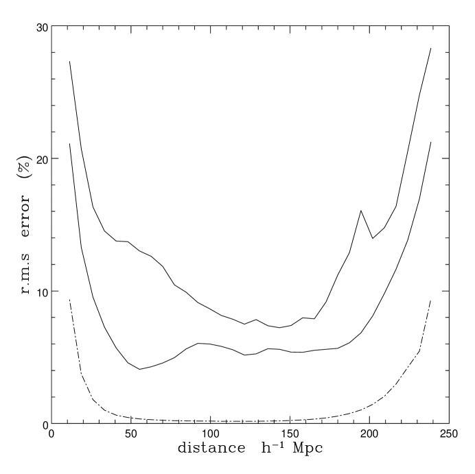
Figure 3: Density reconstruction errors.

Evidently, the reconstruction works well for regions away from the edges of the mock survey in Figure 2. The reconstruction has recovered both the amplitude of the original field and the topology of the isodensity contours. However, a qualitative assessment of the errors is in order. Our focus in this section is on truncation errors as well as errors incurred during interpolation and integration. We estimate the errors with a Monte Carlo method; we realize 72 random density fields, perform reconstruction on each as described above, and determine the r.m.s. point-wise difference between the real density field and the reconstruction. Figure 3 shows the r.m.s. error in reconstruction for points on one of the principle axes of the cubical survey volume (the points lie on a path which bisects the plane shown in Figure 2).

Truncation effects are clear in Figure 3 from the increase in error near the boundary of the survey volume. The truncation error worsens as the correlation length of the density field increases, as can be seen from a comparison of the error curves with correlation lengths of 50 and 100 $h^{-1}$ Mpc (induced by smoothing on those scales); large correlation lengths correspond to low frequency modes which are more susceptible to the ill effects of a finite survey volume.

For the case of the realizations with a smoothing scale of 50 $h^{-1}$ Mpc, we estimate the theoretical truncation error by directly integrating equation (51). The relatively high dimensionality of the integral and the rapid variation of the integrand near the boundaries of the survey volume suggest that this problem is best handled by parallel computation (we are grateful for time on a Cray T-3D at Jet Propulsion Laboratory). For reference, an approximate theoretical error curve is shown in Figure 3. The remaining error comes from grid interpolation, the numerical integrator, and to a lesser extent the breakdown in the Kaiser equation, which is of course only exact for $\delta\ll 1$. This latter source of error scales roughly as $\delta^{2}$, and does become more important at smaller smoothing scales. While in this example we are content to let these errors lie between 5% and 10% near the center of the survey, they may be further reduced with a finer grid mesh and a higher-order integrator.

7 Discussion

We have presented the Green functions for computing the gravitational potential, the peculiar velocity field and the real-space density fluctuations from the distribution of matter in redshift space. Our results are based on Kaiser’s (1987) analysis of redshift-space distortions in the linear regime, and are applicable to surveys of arbitrary geometry.

One virtue of the method presented here is that the entire calculation is performed in real space. This means that the effects of complications such as survey boundaries and the presence of galaxy clusters, which are manifestly in physical space rather than Fourier space, are easy to understand and quantify. For example, the magnitude of the Green function in the parts of space that we are ignoring immediately gives an indication of how much information we are loosing, i.e., on the magnitude of the error bars on the reconstructed field. As we have discussed, this allows the problems caused by shot noise, survey boundaries and nonlinear clustering to be minimized by appropriate choices of the smoothing scale and the integration volume $V$.

We wish to emphasize several possible uses of the Green function method. The first is toward ferreting out estimates of the linear growth parameter $\beta=\Omega^{0.6}/b$. While $\beta$ has been estimated in elegant manners from the correlation anisotropy (e.g., Hamilton 1992), it may also be determined with the Green function ${G_{\delta}}$: The best estimate for $\beta$ is the value which minimizes the anisotropy in the real-space two-point correlation function of the reconstructed field. Quantitative conditions for minimizing the anisotropy in $\xi_{R}$ may be derived with an orthogonal decomposition in spherical harmonics (e.g., Hamilton 1992). For example, a least-squares criterion may be imposed on the amplitudes of terms with spherical harmonics $Y_{lm}$ for which $l>0$, with greatest weights assigned to quadrupole terms, as they couple strongly to the redshift-space distortions.

The second application of the Green function method is to extract information on the nature of biasing. Specifically, the reconstructed real-space density field contains the implicit assumption of a linear bias between luminous and dark matter. Thus it is worth comparing the field with density reconstructions from other techniques such as the POTENT algorithm (Bertschinger & Dekel 1989). While such a comparison will not alone break the degeneracy between $b$ and $\Omega$, it can test the validity of the linear biasing hypothesis.

Ultimately, the method’s most important use is the estimation of peculiar velocities. Even linear peculiar flows can provide stringent constraints on cosmological models (e.g., Lauer & Postman 1994; Tegmark, Bunn & Hu 1994). Since the Green function method generates peculiar velocities directly from redshifts without the difficult measurement of real-space distances, it may have fruitful application in the large-scale digital sky surveys that are currently coming on line.

Our purpose here has been to provide the mathematical underpinnings of the Green function approach to cosmic field reconstruction from redshift data. We are now embarking on the next step, the analysis of redshift surveys.

We thank James Anglin, Marc Davis, Andrew Hamilton, Saleem Zaroubi and our referee for useful comments and suggestions. BCB acknowledges support from the NASA HPCC program and help from Isabel Dulfano.

References

• Bertschinger, E., & Dekel, A. 1989, ApJ, 336, L5

• Bromley, B. C. 1994, ApJ, 423, L81

• Cole, S., Fisher, K. B., & Weinberg, D.  H. 1994, MNRAS, 267, 785

• Efstathiou, G., Bond, J. R., & White, S. D. M. 1992, MNRAS, 258, 1P

• Fisher, K. B., Scharf, C. A., & Lahav, O. 1994, MNRAS, 266, 219

• Giovanelli, R., & Haynes, M. P. 1991, Ann. Rev. Astr. Ap., 29, 499

• Gramann, M., Cen, R. Y. & Gott III, J. R. 1994, ApJ, 425, 382

• Hamilton, A. J. S. 1992, ApJ, 385, L5

• Hamilton, A. J. S. 1993, ApJ, 406, L47

• Kaiser, N. 1987, MNRAS, 227, 1

• Lauer, T. & Postman, M. 1994, ApJ, 425, 418

• Nusser, A. & Davis, M. 1994, ApJ, 421, L1

• Peebles, P. J. E., 1993, Principles of Physical Cosmology (Princeton: Princeton University Press)

• Smoot, G. F. et.al. 1992, ApJ, 396, L1

• Taylor, A. & Rowan-Robinson, M. 1993; MNRAS, 265, 809

• Tegmark, M., Bunn, E., & Hu, W. 1994, ApJ, 434, 1

• Yahil, A., Strauss, M. A., Davis, M., & Huchra, J. P. 1991, ApJ, 372, 380

• Zaroubi, S. & Hoffman, Y. 1994, preprint

Figure 1: The Green functions ${G_{\phi}}$ and ${G_{\delta}}$, for $\beta=1$.

To the left of the $y$-axis are contours of ${G_{\phi}}({\bf r},{\bf r}^{\prime})$, while the contours to the right correspond to ${G_{\delta}}({\bf r},{\bf r}^{\prime})$ for ${\bf r}=(x,y,0)$ and ${\bf r}^{\prime}=(0,1,0)$. The light solid lines and dashed contours indicate positive and negative values, respectively, with logarithmic spacing. The heavy solid line is the ${G_{\delta}}({\bf r})=0$ contour. The trend in both functions is toward high absolute values near the center of the figure. Values of these functions for more general choices of ${\bf r}$ and ${\bf r}^{\prime}$ follow directly from symmetry and scaling properties. The functions essentially give the contribution of a point mass at ${\bf r}$ to the reconstructed field at ${\bf r}^{\prime}$ (point at center of the figure).

Figure 2: An example of the reconstruction method.

As discussed in the text, the reconstruction method is applied to a linearly evolved Gaussian random field in a 250 $h^{-1}$ Mpc cube. The linearly spaced contours, denoting isodensity surfaces at a mid-plane of the cube, show overdensities (solid lines), underdensities (broken lines), and the mean density (heavy solid lines). The observer is located at a corner of the cube. The upper-left plot is the density in real space, generated from a CDM power spectrum with 50 $h^{-1}$ Mpc smoothing. The corresponding redshift-space density (upper-right) is used to reconstruct the real-space fields; the lower-left plot was derived with the correct $\beta$ value while an incorrect value yielded the plot on the lower right.

The r.m.s. reconstruction errors, $\sigma({\bf r})/\sqrt{\xi_{r}(0)}$, are estimated from 72 realizations of a linearly evolved CDM field, with 100 $h^{-1}$ Mpc smoothing (top curve) and 50 $h^{-1}$ Mpc smoothing (middle curve), in the survey region used for Figure 2. The horizontal axis is distance along a principle axis of the cube. The lower (dashed) curve is an estimate of the expected truncation noise, $\sigma_{t}({\bf r})$ for the case of 50 $h^{-1}$ Mpc smoothing.