Abstract

Some of the technical details involved in taking and analyzing data from the COBE are discussed, and recent results from the FIRAS and DMR experiments are summarized. Some of the cosmological implications of these recent data are presented.

1 Introduction

The COBE mission is the product of many years of work by a large team of scientists and engineers. Credit for all of the results presented in these lectures must be shared with the other members of the the COBE Science Working Group: Chuck Bennett, Ed Cheng, Eli Dwek, Mike Hauser, Tom Kelsall, John Mather, Harvey Moseley, Nancy Boggess, Rick Shafer, Bob Silverberg, George Smoot, Steve Meyer, Rai Weiss, Sam Gulkis, Mike Janssen, Dave Wilkinson, Phil Lubin, and Tom Murdock. Bennett et al. (1992a) is an excellent review of the history of the COBE project and its results up to the discovery of the anisotropy by the DMR, but not including the latest FIRAS limits on distortions.

Some of the members of this team have been working on COBE since 1974, when the proposals for what became the COBE project were submitted. I have been working on COBE since the beginning of 1978. COBE was successfully launched on 18 November 1989 from California, and returned high quality scientific data from all three instruments for ten months until the liquid helium ran out. But about 50% of the instruments do not require liquid helium, and are still returning excellent scientific data in January 1993. While the COBE mission has been very successful, making the “discovery of the century”, one must remember that this work is based on the earlier work (in the $20^{th}$ century!) of Hubble (1929) and Penzias and Wilson (1965), who discovered the expansion of the Universe and the microwave background itself. As a consequence of these two discoveries, one knows that the early Universe was very hot and dense. When the density and temperature are high, the photon creation and destruction rates are very high, and are sufficient to guarantee the formation of a very good blackbody spectrum. Later, as the Universe expands and cools, the photon creation and destruction rates become much slower than the expansion rate of the Universe, which allow distortions of the spectrum to survive. In the standard model the time from which distortions could survive is 1 year after the Big Bang at a redshift $z\approx 10^{6.4}$.

However, the action of the expansion itself on a blackbody results in another blackbody with a lower temperature. Thus the existence of a distorted spectrum in the hot Big Bang model requires the existence at time later than 1 year after the Big Bang of both an energy source and an emission mechanism that can produce photons that are now in the millimeter spectral range. Conversely, a lack of distortions can be used to place limits on any such energy source, such as decaying neutrinos, dissipation of turbulence, etc.

At a time $3\times 10^{5}$ years after the Big Bang, at $z\approx 10^{3}$, the temperature has fallen to the point where helium and then hydrogen (re)combine into transparent gases. The electron scattering which had impeded the free motion of the CMB photons until this epoch is removed, and the photons stream across the Universe. Before recombination, the radiation field at any point was constrained to be very nearly isotropic because the rapid scattering scrambled the directions of photons. The radiation field was not required to be homogeneous, because the photons remained approximately fixed in comoving co-ordinates. After recombination, the free streaming of the photons has the effect of averaging the intensity of the microwave background over a region with a size equal to the horizon size. Thus after recombination any inhomogeneity in the microwave background spectrum is smoothed out. Note that this inhomogeneity is not lost: instead, it is converted into anisotropy. When we study the isotropy of the microwave background, we are looking back to the surface of last scattering 300,000 years after the Big Bang. But the hot spots and cold spots we are studying existed as inhomogeneities in the Universe before recombination. Since the $7^{\circ}$ beam used by the DMR instrument on COBE is larger than the horizon size at recombination, these inhomogeneities cannot be constructed in a causal fashion during the epoch before recombination in the standard Big Bang model. Instead, they must be installed “just so” in the initial conditions. In the inflationary scenario of Guth (1980), these large scale structures were once smaller than the horizon size during the inflationary epoch, but grew to be much larger than the horizon. Causal physics acting $10^{-35}$ seconds after the Big Bang can produce the large-scale inhomogeneities studied by the DMR.

2 COBE Orbit and Attitude

COBE was launched at 0634 PST on 18 November 1989 into a sun-synchronous orbit with an inclination of $99^{\circ}$ and an altitude of 900 km. By choosing a suitable combination of inclination and altitude, the precession rate of the orbit can be set to follow the motion of the Sun around the sky at 1 cycle per year. The gravitational potential energy of the satellite, averaged over its orbit, has an inclination dependence due to the equatorial bulge of the Earth that is proportional to

$$\Delta E\propto\frac{-m\cos^{2}i}{a^{3}}$$ (1)

where $m$ is the mass of COBE, which produces a torque $T=-\partial E/\partial i\propto 2ma^{-3}\cos i\sin i$. The perpendicular component of the angular momentum of the satellite in its orbit is proportional to

$$L_{\perp}\propto m\sin i\sqrt{a}.$$ (2)

The precession rate is determined by $\omega_{P}=T/L_{\perp}$ which is thus

$$\omega_{P}\approx\left(-10^{\circ}/{\rm day}\right)\cos i(R_{\oplus}/a)^{3.5}$$ (3)

where the minus sign indicates a retrograde precession. The choice $i=99^{\circ}$, or $\cos i=-0.156$, with $a=R_{\oplus}+900\;{\rm km}=7271\;{\rm km}$, gives the proper precession rate.

Since COBE was launched toward the South in the morning, the end of the orbit normal which points toward the Sun is at declination $-9^{\circ}$. At the June solstice, when the declination of the Sun is $+23^{\circ}$, there is a $32^{\circ}$ deviation from the ideal situation where the Earth-Sun line is exactly perpendicular to the orbit. Since the depression of the horizon given by $\cos d=R_{\oplus}/a$ is $29^{\circ}$, there are eclipses when COBE passes over the South pole for a period of two months centered on the June solstice. During the same season at the North pole the angle between the Sun and anti-Sunward limb of the Earth is only $177^{\circ}$. It is thus not possible to keep both Sunlight and Earthshine out of the shaded cavity around the dewar. Since the Sun produces a much greater bolometric intensity than a thin crescent of Earth limb, the choice to keep the Sun below the plane of the shade is an obvious one.

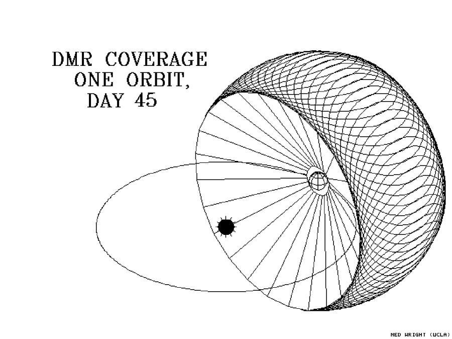
Figure 1: The DMR scan pattern for one orbit covers the band from $64^{\circ}$ to $124^{\circ}$ from the Sun.

The pointing of COBE is normally set to maintain the angle between the spin axis and the Sun at $94^{\circ}$. This leaves the Sun $4^{\circ}$ below the plane of the shade. During eclipse seasons this margin is shaved to $2^{\circ}$ to reduce the amount of Earthshine into the shaded cavity where the instruments sit. The angle between the plane of the shade and the Sun is known as the “roll” angle. The “pitch” angle describes the rotation of the spin axis around the Earth-Sun line. This rotation is programmed for a constant angular rate of 1 cycle per orbit. The nadir is set to be close to the minus spin axis, but because the Sun can be up to $32^{\circ}$ from the orbit normal and the Sun is kept $4^{\circ}$ below the plane of the shade, the spin axis can be up to $36^{\circ}$ away from the zenith. The uniform rate in pitch allows the nadir to oscillate by up to $\pm 6^{\circ}$ relative to the spin-Sun plane with a period of 2 cycles per orbit. This motion is similar to the effect of the inclination of the ecliptic on the equation of time that can be seen in an analemma. To keep the “wind” caused by the orbital motion of COBE from impinging on the cryogenic optics, the pitch is biased backward by $6^{\circ}$. The “yaw” motion of COBE is its spin. The spin period is about 73 seconds.

There are two types of instrument pointings on COBE. The FIRAS points straight out along the spin axis. As a result its field-of-view moves only at the orbital rate of $3.6^{\circ}/{\rm min}$. Since FIRAS coadds interferograms over a collection period of about 30 to 60 seconds, this slow scanning of the sky is essential. The DMR and DIRBE instruments have fields-of-view located $30^{\circ}$ away from the spin axis. As a result they scan cycloidal paths through the sky, that cover the band from $64^{\circ}$ to $124^{\circ}$ from the Sun. This band contains 50% of the sky, and it is completely covered in a day by the DMR or DIRBE. Figure 1 shows the DMR scan pattern schematically. This rapid coverage of the sky implies a rapid scan rate: $2.5^{\circ}/{\rm sec}$. The data rates are also high: the DIRBE transmits 8 readings/channel/sec, while the DMR transmits 2 readings/channel/sec.

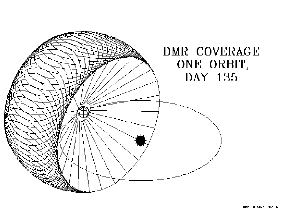
Figure 2: The DMR scan pattern 3 months later with the Sun in a different position.

Over the course of a year the Sun moves around the sky, and the scan paths of the instruments follow this motion. The leading edge of the wide scanned band for the DIRBE and DMR caught up to the trailing edge of the band at start of mission after 4 months, leading to 100% sky coverage. Figure 2 shows the DMR scan pattern 3 months after the situation shown in Figure 1. For the FIRAS total sky coverage would in principle be obtained after 6 months, but because of gaps in the observations caused by calibration runs and lunar interference, the actual sky coverage for FIRAS, defined as having the center of the beam within a pixel, is about 90%. The coverage gaps are sufficiently narrow, however, that every direction on the sky was covered by at least the half power contour of the beam.

3 FIRAS Measurements

The Far InfraRed Absolute Spectrophotometer instrument on COBE is a polarizing Michelson or Martin-Puplett (1970) interferometer. The optical layout is very symmetrical, and it has two inputs and two outputs. If the two inputs are denoted SKY and ICAL, then the two outputs, which are denoted LEFT and RIGHT, are given symbolically as

$${\rm LEFT} = {\rm SKY}-{\rm ICAL}$$ (4)

$${\rm RIGHT} = {\rm ICAL}-{\rm SKY}$$ (5)

The FIRAS has achieved its incredible sensitivity to small deviations from a blackbody spectrum by connecting the ICAL input to an internal calibrator, a reference blackbody that can be set to a temperature very close to the temperature $T_{\circ}$ of the sky. Thus this “absolute” spectrophotometer is so successful because it is differential. In addition, each output is further divided by a dichroic beamsplitter into a low frequency channel (2-21 ${\rm cm}^{-1}$) and a high frequency channel (23-95 ${\rm cm}^{-1}$). Thus there are four overall outputs. These are labeled LL (left low) through RH (right high).

Each output has a large composite bolometer that senses the output power by absorbing the radiation, converting this power into heat, and then detecting the temperature rise of a substrate using a very small and sensitive silicon resistance thermometer. In order to minimize the specific heat of the bolometer, which maximizes the temperature rise for a given input power, the substrate is made of the material with the highest known Debye temperature: diamond. Diamond is quite transparent to millimeter waves, however, so an absorbing layer is needed. Traditionally a layer of bismuth has been used as the absorber on composite bolometers, but the FIRAS detectors use a very thin layer of gold alloyed with chromium. The absorbing layer needs to have a surface impedance about one-half of the 377 Ohms/$\Box$ impedance of free space in order to absorb efficiently, and this surface impedance can be obtained with a much thinner layer of gold rather than bismuth. Again, this serves to minimize the specific heat of the detector. In order to detect the longest waves observed by FIRAS, the diameter of the octagonal diamond substrate is quite large: about 8 mm. Each detector sits behind a compound parabolic concentrator, or Winston cone, which provides a full $\pi$ steradians in the incoming beam. As a result, the FIRAS instrument has a very large étendue of 1.5 cm${}^{2}\;$sr.

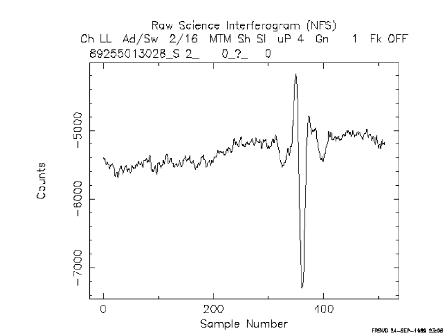
Figure 3: A FIRAS interferogram from the Left Low channel taken during ground test with the XCAL at 2.2 K and the ICAL at 2.7 K

Since the FIRAS is a Michelson interferometer, the spectral data is obtained in the form of interferograms. Thus the LEFT output is approximately

$$I_{L}(x)=\int_{0}^{\infty}\cos(2\pi\nu x)G(\nu)\left(I_{\nu}+\sum_{i}\epsilon_{i}(\nu)B_{\nu}(T_{i})+U_{\nu}\right)d\nu$$ (6)

The index $i$ above runs over all the components in the FIRAS that had thermometers to measure $T_{i}$. These include the ICAL, the reference horn that connects to the ICAL, the sky horn, the bolometer housing, the optical structure of the FIRAS, and the dihedral mirrors that move to provide the variation in path length difference $x$. The $\epsilon_{i}$’s are the effective emissivities of the various components. The ICAL itself has $\epsilon\approx-1$, while the sky and reference horns have $\epsilon$’s of $\pm$ a few percent. The offset term $U_{\nu}$ was observed during flight to be approximately $10^{-5}\exp(-t/\tau)B_{\nu}(T_{U})$ with a time constant $\tau$ of two months and a temperature $T_{U}\approx 15$ K. The SKY input $I_{\nu}$ above can be either the sky or an external calibrator. The XCAL is a movable re-entrant absorber that can be inserted at the top of the sky horn. The combination of sky horn plus XCAL forms a cavity with an absorbtivity $>0.999$, and we believe ${{}_{>}\atop{}^{\sim}}0.99999$. With the XCAL inserted during periodic calibration runs, the SKY input is known to be $B_{\nu}(T_{X})$. By varying $T_{X}$ and the other $T_{i}$’s, the calibration coefficients have been determined. See Fixsen et al. (1993a) for a more complete description of the calibration procedure. Figure 3 shows an interferogram from ground testing with the ICAL at 2.7 K and the XCAL at 2.2 K.

Once the calibration coefficients are known, the sky data can be analyzed to determine $I_{\nu}(l,b)$ the intensity of the sky as a function of frequency, galactic longitude and galactic latitude. This is a “data cube”. The data from each direction on the sky can be written as a combination of cosmic plus galactic signals:

$$I_{\nu}(l,b) = e^{-\tau_{\nu}(l,b,\infty)}\left(B_{\nu}\left(T_{\circ}+\Delta T(l,b)\right)+\Delta I_{\nu}\right)$$ (7)

$$+ \int e^{-\tau_{\nu}(l,b,s)}j_{\nu}(l,b,s)ds$$

where $\tau_{\nu}(l,b,s)$ is the optical depth between the Solar system and the point at distance $s$ in the direction $(l,b)$ at frequency $\nu$, $\Delta I_{\nu}$ is an isotropic cosmic distortion, and $\Delta T(l,b)$ is the variation of the background temperature around its mean value $T_{\circ}$. This equation can be simplified because the optical depth of the galactic dust emission is always very small in the millimeter and sub-millimeter bands covered by FIRAS.

$$I_{\nu}(l,b)\approx B_{\nu}\left(T_{\circ}+\Delta T(l,b)\right)+\Delta I_{\nu}+\int j_{\nu}(l,b,s)ds$$ (8)

Even in the optically thin limit, some restrictive assumptions about the galactic emissivity $j_{\nu}$ are needed, since the galactic intensity $\int j_{\nu}(l,b,s)ds$ is a function of three variables, just like the observed data. The simplest reasonable model for the galactic emission is the one used in Wright et al. (1991): let

$$\int j_{\nu}(l,b,s)ds=G(l,b)g(\nu).$$ (9)

This model assumes that the shape of the galactic spectrum is independent of direction on the sky. It is reasonably successful except that the galactic center region is clearly hotter than the rest of the galaxy. The application of this model proceeds in two steps. The first step assumes that the cosmic distortions vanish, and that an approximation $g_{\circ}(\nu)$ to the galactic spectrum is known. A least squares fit over the spectrum in each pixel then gives the maps $\Delta T(l,b)$ and $G(l,b)$. The high frequency channel of FIRAS is used to derive $G(l,b)$ because the galactic emission is strongest there. An alternative way to derive $G(l,b)$ is to smooth the DIRBE map at 240 ${\rm\mu m}$ to the FIRAS $7^{\circ}$ beam. This DIRBE method has been used in the latest FIRAS spectral results in Mather et al. (1993), Fixsen et al. (1993b) and Wright et al. (1993). The second step in the galactic fitting then derives spectra associated with the main components of the millimeter wave sky: the isotropic cosmic background, the dipole anisotropy, and the galactic emission. This fit is done by fitting all the pixels (except for the galactic center region with $|b|<20$ and $|l|<40$) at each frequency to the form

$$I_{\nu}(l,b)=I_{\circ}(\nu)+D(\nu)\cos\theta+G(l,b)g(\nu).$$ (10)

The spectra of the anisotropic components derived from this fit applied to the entire mission data set are shown in Figures 4 and 5. Figure 5 shows the residual after the predicted dipole spectrum $\Delta T\partial B_{\nu}/\partial T$ evaluated at $T_{\circ}$ is subtracted from $D(\nu)$.

But the FIRAS calibration model is so complicated and the cosmic distortions, if any, are so small, that there are still systematic uncertainties that limit the accuracy of the isotropic spectrum $I_{\circ}(\nu)$ derived from the whole FIRAS data set. Therefore the best estimate of $I_{\circ}(\nu)$ comes from the last six weeks of the mission, when a modified observing sequence consisting of 3.5 days of observing the sky with the ICAL set to null out the cosmic spectrum, followed by 3.5 days of observing the XCAL with its temperature set to match the sky temperature $T_{\circ}$. Six cycles of this alternation between sky and XCAL were obtained before the helium ran out. By processing both the sky data and the XCAL data through the same calibration model, and then subtracting the two spectra, almost all of the systematic errors cancel out. The residual in the high galactic latitude sky is then modeled as

$$I_{\nu}(sky,|b|>b_{c})-I_{\nu}(XCAL)=\Delta I_{\nu}+\delta T\frac{\partial B_{\nu}}{\partial T}+Gg(\nu).$$ (11)

The result of a least squares fit to minimize $\Delta I_{\nu}$ by adjusting $\delta T$ and $G$ is shown in Figure 4. The data points show the residuals while the curves show the “uninteresting” models $\partial B_{\nu}/\partial T$ and $g(\nu)$. It is important to remember that any cosmic distortion with a spectral shape that matches one of these curves will be hidden in this fit. The maximum residual between 2 and 20 ${\rm cm}^{-1}$ is 1 part in 3000 of the peak of the blackbody, and the weighted RMS residual is 1 part in $10^{4}$ of the peak of the blackbody. While these residuals are very small, they are nonetheless more than twice the residuals that one would expect from detector noise alone. The error bars in Figure 4 have been inflated by a constant factor to give $\chi^{2}=32$ for the 32 degrees of freedom in the fit. Limits on cosmological distortions can now be set by adding terms to the above fit, finding the best fit value with minimum $\chi^{2}$, and then finding the endpoints of the 95% confidence interval where $\chi^{2}=\chi^{2}_{min}+4$. As an example of such a fit, suppose that the sky in fact was a gray-body with an emissivity $\epsilon=1+e$, where $e$ is a small parameter. Since the XCAL is a good blackbody, this model predicts a residual of the form $eB_{\nu}(T_{\circ})$. Because $B_{\nu}(T_{\circ})$ peaks at a lower frequency than $\partial B_{\nu}/\partial T$, this model is sufficiently different from the “uninteresting” models and a tight limit on $e$ can be set: $|e|<0.00041$ (95% confidence). The result of fits for the usual cosmological suspects are $|y|<2.5\times 10^{-5}$ and $|\mu|<3.3\times 10^{-4}$ with 95% confidence.

Figure 4: FIRAS residuals (points) after fitting for a blackbody and galactic emission, with an 0.5 mK $\Delta T$ and a $\Delta(\csc|b|)=0.25$ galaxy curve shown for comparison. Full-scale is 0.1% of the peak of the CMB.

The absolute temperature of the cosmic background, $T_{\circ}$, can be determined two ways using FIRAS. The first way is to use the readings of the germanium resistance thermometers in the XCAL when the XCAL temperature is set to match the sky. This gives $T_{\circ}=2.730$ K. The second way is to measure the frequency of the peak of $\partial B_{\nu}/\partial T$ by varying $T_{X}$ by small amounts around the temperature which matches the sky, and then apply the Wien displacement law to convert this frequency into a temperature. This calculation is done automatically by the calibration software, and it gives a value of 2.722 K for $T_{\circ}$. The final adopted value is $2.726\pm 0.010$ K (95% confidence), which just splits the difference between the two methods.

Figure 5: FIRAS Dipole spectrum residuals (points). Full-scale is 0.1% of the peak of the CMB.

4 FIRAS Interpretation

When interpreting the implications of the FIRAS spectrum on effects that could distort the microwave background, it is important to remember some basic order-of-magnitude facts. Theoretical analyses of light element abundances gives limits on the current density of baryons through models of Big Bang NucleoSynthesis (BBNS). Walker et al. (1991) give a ratio of baryons to photons of $\eta=(3.5\pm 0.7)\times 10^{-10}$, while Steigman and Tosi (1992) give $\eta=(3.95\pm 0.25)\times 10^{-10}$. Since the number density of photons is well determined by the FIRAS spectrum

$$N=8\pi\zeta(3)\Gamma(3)\left(\frac{kT_{\circ}}{hc}\right)^{3}=410\pm 5\;{{\rm cm}^{-3}}$$ (12)

the baryon density is well determined: $1.62\times 10^{-7}\;{{\rm cm}^{-3}}$. This gives $\Omega_{B}h^{2}=0.0144$, where $h=H_{\circ}/(100\;{\rm km/sec/Mpc})$. Not all of these baryons are protons, however. For a primordial helium abundance of 23.5% by mass, one has 13 protons and 1 $\alpha$ particle in 17 baryons. This gives an electron density of $n_{e,\circ}=1.43\times 10^{-7}\;{{\rm cm}^{-3}}$. For a fully ionized Universe, the optical depth for electron scattering over a path length equal to the Hubble radius $c/H_{\circ}$ is $0.00088/h$.

The expansion of the Universe $H$ varies with time and redshift in a way that depends on ratios of the current matter, radiation and vacuum densities to the critical density $\rho_{c}=3H^{2}/8\pi G$. Let these ratios be $\Omega_{m}$, $\Omega_{r}$, and $\Omega_{v}$. Then

$$H(z)=(1+z)H_{\circ}\sqrt{(1-\Omega_{m}-\Omega_{r}-\Omega_{v})+\Omega_{m}(1+z)+\Omega_{r}(1+z)^{2}+\Omega_{v}(1+z)^{-2}}$$ (13)

This equation is not exact for massive neutrinos which shift from being part of $\Omega_{m}$ into part of $\Omega_{r}$ as $z$ increases. The value of $\Omega_{r}h^{2}=(4.16\pm 0.06)\times 10^{-5}$ is fairly well-determined for the case of three massless neutrinos. Thus if $\Omega_{m}\approx 1$ now, the Universe becomes radiation dominated for $z>z_{eq}=2.4h^{2}\times 10^{4}$ when the background temperature was $kT_{eq}=5.65h^{2}\;{\rm eV}$. In the radiation dominated epoch, $H=0.645(1+z)^{2}\;{\rm km/sec/Mpc}$ or $H=2.09(1+z)^{2}\times 10^{-20}\;{\rm s}^{-1}$.

For early epochs when the Universe was ionized, electron scattering is the dominant mechanism for transferring energy between the radiation field and the matter. As long as the electron temperature is less than about $10^{8}$ K, the effect of electron scattering on the spectrum can be calculated using the Kompaneets equation:

$$\frac{\partial n}{\partial y}=x^{-2}\frac{\partial}{\partial x}\left[x^{4}\left(n+n^{2}+\frac{\partial n}{\partial x}\right)\right]$$ (14)

where $n$ is the number of photons per mode ($n=1/(e^{x}-1)$ for a blackbody), $x=h\nu/kT_{e}$, and the Kompaneets $y$ is defined by

$$dy=\frac{kT_{e}}{m_{e}c^{2}}n_{e}\sigma_{T}cdt.$$ (15)

Thus $y$ is the electron scattering optical depth times the electron temperature in units of the electron rest mass. Note that the electrons are assumed to follow a Maxwellian distribution, but that the photon spectrum is completely arbitrary.

Since the Kompaneets equation is describing electron scattering, which preserves the number of photons, one finds that the $y$ derivative of the photon density $N$ vanishes:

$$\frac{\partial N}{\partial y} \propto \int x^{2}\frac{\partial n}{\partial y}dx$$ (16)

$$= \int\frac{\partial}{\partial x}\left[x^{4}\left(n+n^{2}+\frac{\partial n}{\partial x}\right)\right]dx$$

$$= 0$$

The stationary solutions of the equation $\partial n/\partial y=0$ are the photon distributions in thermal equilibrium with the electrons. Since photons are conserved, the photon number density does not have to agree with the photon number density in a blackbody at the electron temperature. Thus a more general Bose-Einstein thermal distribution is allowed: $n=1/(\exp(x+\mu)-1)$. This gives $\partial n/\partial y=0$ for all $\mu$. Since the Bose-Einstein spectrum is a stationary point of the Kompaneets equation, it is the expected form for distortions produced at epochs when

$$(1+z)\frac{\partial y}{\partial z}=\sigma_{T}n_{e,\circ}\frac{kT_{\circ}}{m_{e}c^{2}}\frac{c}{H}(1+z)^{4}>1$$ (17)

For the $\Omega_{B}h^{2}$ given by BBNS, this redshift $z_{y}$ where this inequality is crossed is well within the radiation dominated era, with a value $z_{y}=10^{5.1}/\sqrt{70\Omega_{B}h^{2}}$.

There are two simple solutions to the Kompaneets equation with non-zero $\partial n/\partial y$ which both give the same spectral distortion. The first simple case occurs when the electron temperature is much higher than the typical photon energy. This is the case for clusters of galaxies today with $T_{e}\approx 10^{8}$ K, or for a hot intergalactic medium. Since the variable $x$ in the Kompaneets equation is the photon energy measured in units of the electron thermal energy, $x$ and hence $\Delta x$ are both very small in this case. Therefore the $\partial n/\partial x$ term in the Kompaneets equation is much larger than the $n$ or $n^{2}$ terms which may be dropped. This gives a simpler equation

$$\frac{\partial n}{\partial y}=x^{-2}\frac{\partial}{\partial x}\left[x^{4}\left(\frac{\partial n}{\partial x}\right)\right]$$ (18)

which was used by Sunyaev and Zeldovich. Note that the powers of $x$ on the right hand side cancel out, so the RHS can be evaluated using $x=h\nu/kT_{\gamma}$ if the initial photon field is a blackbody with temperature $T_{\gamma}$. The solution is easily evaluated and usually expressed in terms of a frequency dependent brightness temperature:

$$\frac{\partial T}{\partial y}=T_{\gamma}\left(\frac{x(e^{x}+1)}{e^{x}-1}-4\right).$$ (19)

The second simple case occurs when the initial photon field is a blackbody with a temperature $T_{\gamma}$ which is only slightly below the electron temperature. Letting $f=T_{e}/T_{\gamma}$, we find that the initial photon field is given by $n=1/(\exp(fx)-1)$. Therefore

$$\left(n+n^{2}+\frac{\partial n}{\partial x}\right)=\frac{(1-f)\exp(fx)}{(\exp(fx)-1)^{2}}=(1-f^{-1})\frac{\partial n}{\partial x}.$$ (20)

Thus the distortion has a Sunyaev-Zeldovich shape but is reduced in magnitude by a factor $(1-T_{\gamma}/T_{e})$. Defining the “distorting” $y$ as

$$dy_{D}=\frac{k(T_{e}-T_{\gamma})}{m_{e}c^{2}}n_{e}\sigma_{T}cdt$$ (21)

we find that the final spectrum is given by a frequency-dependent temperature given by

$$T_{\nu}=T_{\circ}\left[1+y_{D}\left(\frac{x(e^{x}+1)}{e^{x}-1}-4\right)+\ldots\right].$$ (22)

where $x=h\nu/kT_{\circ}$. The FIRAS spectrum in Figure 4 shows that $|y_{D}|<2.5\times 10^{-5}$.

The energy density transferred from the hotter electrons to the cooler photons in the $y$ distortion is easily computed. The energy density is given by $U\propto\int x^{3}ndx$ so

$$\frac{\partial U}{\partial y_{D}}=\int x\frac{\partial}{\partial x}\left(x^{4}\frac{\partial n}{\partial x}\right)dx$$ (23)

which when integrated by parts twice gives

$$\frac{\partial U}{\partial y_{D}} = -\int\left(x^{4}\frac{\partial n}{\partial x}\right)dx$$ (24)

$$= 4\int x^{3}ndx=4U.$$

Thus the limit on $y_{D}$ gives a corresponding limit on energy transfer: $\Delta U/U<10^{-4}$. Any energy which is transferred into the electrons at redshifts $z>7$ where the Compton cooling time is less than the Hubble time will be transferred into the photon field and produce a $y$ distortion. Since there are $10^{9}$ times more photons that any other particles except for the neutrinos, the specific heat of the photon gas is overwhelmingly dominant, and the electrons rapidly cool (in a Compton cooling time) back into equilibrium with the photons. The energy gained by the photons is $\Delta U=4yaT_{\gamma}^{4}$ which must be equal to the energy lost by the electrons and ions: $1.5(n_{e}+n_{i})k\Delta T_{e}$. Since $y=\sigma_{T}n_{e}(kT_{e}/m_{e}c^{2})c\Delta t$ we find the Compton cooling time

$$t_{C}=\frac{1.5(1+n_{i}/n_{e})m_{e}c^{2}}{4\sigma_{T}cU_{rad}}=\frac{7.4\times 10^{19}\;{\rm sec}}{(1+z)^{4}}$$ (25)

for an ion to electron ratio of $14/15$. This becomes equal to the Hubble time $(3.08568\times 10^{17}{\rm sec})/(h(1+z)^{1.5})$ at $(1+z)=9h^{0.4}$.

At redshifts $z>z_{y}=10^{5}$, there will be enough electron scattering to force the photons into a thermal distribution with a $\mu$ distortion instead of a $y$ distortion. However, the normal form for writing a $\mu$ distortion does not preserve the photon number density. Thus we should combine the $\mu$ distortion with a temperature change to give an effect that preserves photon number. The photon number density change with $\mu$ is given by

$$N \propto \int{\frac{x^{2}dx}{\exp(x+\mu)-1}}$$ (26)

$$= \sum_{k=1}^{\infty}e^{-k\mu}\int x^{2}e^{-kx}dx$$

$$= 2\sum_{k=1}^{\infty}{\frac{e^{-k\mu}}{k^{3}}}$$

$$= 2\left(\zeta(3)-\mu\zeta(2)+\ldots\right).$$

A similar calculation for the energy density shows that

$$U\propto 6\left(\zeta(4)-\mu\zeta(3)+\ldots\right).$$ (27)

In order to maintain $N=const$, the temperature of the photon field changes by an amount $\Delta T/T=\mu\zeta(2)/(3\zeta(3))$. Therefore, the energy density change at constant $N$ is

$$\frac{\Delta U}{U}=\left(\frac{4\zeta(2)}{3\zeta(3)}-\frac{\zeta(3)}{\zeta(4)}\right)\mu=0.714\mu.$$ (28)

Thus the FIRAS limit $|\mu|<3.3\times 10^{-4}$ implies $\Delta U/U<2.4\times 10^{-4}$. The “improved” form of the $\mu$ distortion, with a $\Delta T$ added to keep $N$ constant, can be given as a frequency dependent brightness temperature:

$$T_{\nu}=T_{\circ}\left(1+\mu\left[\frac{\zeta(2)}{3\zeta(3)}-x^{-1}\right]+\ldots\right).$$ (29)

In this form it is clear that a $\mu$ distortion has a deficit of low energy photons and a surplus of high energy photons with respect to a blackbody. In this it is like the $y$ distortion, but the crossover frequency is lower.

Finally, at high enough redshift the process of double photon Compton scattering becomes fast enough to produce the extra photons needed to convert a distorted spectrum into a blackbody. Whenever a photon with frequency $\nu$ scatters off an electron, there is an impulse $\propto h\nu/c$ transferred to the electron. This corresponds to an acceleration $a\propto h\nu^{2}/(m_{e}c)$ for a time interval $\Delta t\propto 1/\nu$. The energy radiated in new photons is thus $\propto e^{2}h^{2}\nu^{3}/(m_{e}^{2}c^{5})$ which is $\propto\alpha h\nu(h\nu/(m_{e}c^{2}))^{2}$. Since the rate of scatterings per photon is $\propto\Omega_{B}h^{2}(1+z)^{3}$, the overall rate of new photon creation is $\propto\Omega_{B}h^{2}(1+z)^{5}$ while the Hubble time is $\propto(1+z)^{-2}$. Burigana, De Zotti & Danese (1991) properly consider the interaction of this photon creation process with the Kompaneets equation and show that the redshift from which $1/e$ of an initial distortion can survive is

$$z_{th}=\frac{4.24\times 10^{5}}{\left[\Omega_{B}h^{2}\right]^{0.4}}$$ (30)

which is $z_{th}=2.3\times 10^{6}$ for the BBNS value of $\Omega_{B}h^{2}$.

5 DMR Observations

The Differential Microwave Radiometers (DMR) experiment on COBE is designed to measure small temperature differences from place to place on the sky. The DMR consist of three separate units, one for each of the three frequencies of 31.5, 53 and 90 GHz. The field of view of each unit consists of two beams that are separated by a $60^{\circ}$ angle that is bisected by the spin axis. Each beam has a $7^{\circ}$ FWHM. The DMR is only sensitive to the brightness difference between these two beams. This differencing is performed by a ferrite waveguide switch that connects the receiver input to one horn and then the other at a rate of 100 cycles per second. The signal then goes through a mixer, an IF amplifier and a video detector. The output of the video detector is demodulated by a lock-in amplifier synchronized to the input switch. The difference signal that results is telemetered to the ground every 0.5 seconds. Each radiometer has two channels: A and B. In the case of the 31.5 GHz radiometer, the two channels use a single pair of horns in opposite senses of circular polarization. In the 53 and 90 GHz radiometers there are 4 horns, and all observe the same sense of linear polarization.

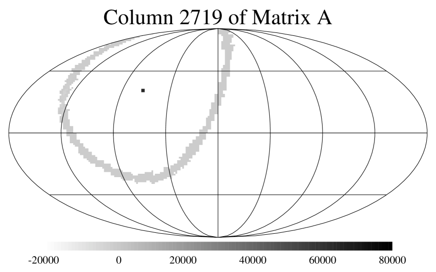
Figure 6: The column through pixel 2719 of the sparse matrix A from a 2 year simulation.

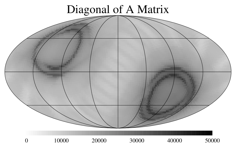
Figure 7: The diagonal of the sparse matrix A, otherwise known as the coverage map, from a 1 year simulation.

The basic problem in the DMR data analysis is to construct a map of the sky using the $6\times 10^{7}$ differences that are collected each year. There are only about $10^{3}$ beam areas on the sky, so the problem is highly over-determined. We have chosen to analyze the data using 6,144 pixels to cover the sky. These are approximately equal area, and arranged in a square grid of $32\times 32$ pixels on each of the 6 faces of a cube. Within each pixel we assume that the temperature is constant, so we are modeling the sky with a staircase function. Therefore the basic problem can be represented as a least-squares problem with $6\times 10^{7}$ equations in 6,144 variables. Each equation has the form $S_{k}=V_{k}X$ where the column vector $X$ is the map we wish to find, while the row vector $V_{k}=[0,\ldots,0,+1,0,\ldots,0,-1,0,\ldots]$ with the $+1$ in the pixel which contained the plus beam and the $-1$ in the pixel that contained the minus beam at the time of the $k^{th}$ observation $S_{k}$. Then the normal least-squares equations are found using

$$A = \sum_{k}V_{k}^{T}V_{k}$$

$$B = \sum_{k}S_{k}V_{k}^{T}$$

$$X = lim_{\epsilon\rightarrow 0^{+}}\left(A+\epsilon I\right)^{-1}B$$ (31)

Note that $A$ is sparse and symmetric. While $A$ has $38\times 10^{6}$ elements, all but $1.8\times 10^{6}$ of these elements are zero, and $A_{ij}=A_{ji}$. Thus only $9\times 10^{5}$ elements need to be kept.

Visualizing a matrix with so many elements is difficult, but we can convert a given row (or column by symmetry) into a map. Figure 6 shows a column of the $A$ matrix. The pixel on the diagonal is number 2719, and it is one of the most heavily observed pixels in the rings $30^{\circ}$ from the ecliptic poles. The diagonal of the $A$ matrix can also be made into a map: it is the coverage map showing the number of observations in each pixel (Figure 7).

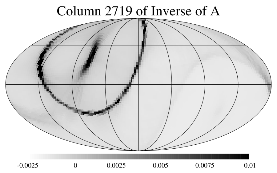
Figure 8: The column through pixel 2719 of the normalized inverse of A. The diagonal pixel 2719 is saturated with a value of 1.03

Adding $\epsilon I$ to $A$ allows for the fact that the sum or mean of the map cannot be determined from the DMR data. This is equivalent to having one observation per pixel with weight $\epsilon$ which states that the pixel value is zero. Since there are $\approx 10^{4}$ observations per pixel, with unit weight corresponding to an error of about 25 mK, and the map values are all $<4$ mK, rather large values of $\epsilon\approx 10^{3}$ could be used without affecting the maps, while the iterative algorithm used to find $X$ is quite stable even for $\epsilon\approx 10^{-3}$. An alternative method that can be used to regularize the inverse of $A$ is to add a matrix of all 1’s to $A$. This is equivalent to one observation stating that the sum of the map is zero. Both methods give the same answer for fully-covered sky maps, but the $\epsilon I$ approach converges better for partial sky maps. Figure 8 shows the result when $B$ above is replaced by the column vector with elements $(-1,\ldots,-1,6143,-1,\ldots,-1)\times(N_{2719}/6144)$, where the positive element is at pixel 2719, and $N_{2719}$ is the number of observations at the $2719^{th}$ pixel. The value of the central pixel in this map is 1.03 which indicates that the conversion of the observed differences into a map value has increased the variance by 3%. The values of about 0.01 or less in the $60^{\circ}$ radius reference ring indicates the extent to which noise in the reference ring affects the map values. These pixel-pixel correlations are quite small and have very little effect on any analyses except for the autocorrelation function of maps at $60^{\circ}$ separation.

6 DMR Results

Smoot et al. (1992), Wright et al. (1992), Bennett et al. (1992b) and Kogut et al. (1992) announced the basic DMR result: the discovery of an intrinsic anisotropy of the microwave background, beyond the dipole anisotropy discovered by Conklin (1969). This anisotropy, when a monopole and dipole fit to $|b|>20^{\circ}$ is removed from the map, and the map is then smoothed to a resolution of $\approx 10^{\circ}$, is 30 ${\rm\mu K}$. The correlation function of this anisotropy is well fit by the expected correlation function for the Harrison-Zeldovich spectrum of primordial density perturbations predicted by the inflationary scenario. The ratio of the gravitational potential fluctuations seen by the DMR through the Sachs-Wolfe (1967) effect to the gravitational potentials inferred from the bulk flows of galaxies using the POTENT method (Bertschinger et al. (1990)), shows that the Harrison-Zeldovich spectrum has the correct slope to connect the DMR data at $3\times 10^{5}$ km/sec scales to the bulk flow data at 6000 km/sec scale.

Figure 9: The current gravitational potential perturbations for the 4 models from Holtzman (1989) that were called out in Wright et al. 1992.

Wright et al. (1992) discussed the implications of the COBE DMR data for models for structure formation, and selected 4 models from the large collection in Holtzman (1989) for detailed discussion: a “CDM” model, with $H_{\circ}=50\;{{\rm km}\;{\rm s}^{-1}\;{\rm Mpc}^{-1}}$, $\Omega_{CDM}=0.9$, and $\Omega_{B}=0.1$; a mixed“CDM+HDM” model, with $H_{\circ}=50\;{{\rm km}\;{\rm s}^{-1}\;{\rm Mpc}^{-1}}$, $\Omega_{CDM}=0.6$, $\Omega_{HDM}=0.3$ (a 7 eV neutrino), and $\Omega_{B}=0.1$; an open model, with $H_{\circ}=100\;{{\rm km}\;{\rm s}^{-1}\;{\rm Mpc}^{-1}}$, $\Omega_{CDM}=0.18$, and $\Omega_{B}=0.02$; and a vacuum dominated model, with $H_{\circ}=100\;{{\rm km}\;{\rm s}^{-1}\;{\rm Mpc}^{-1}}$, $\Omega_{CDM}=0.18$, $\Omega_{B}=0.02$, and $\Omega_{vac}=0.8$. The vacuum dominated model and especially the open model have potential perturbations now that are too small to explain the Bertschinger et al. bulk flow observation, as seen in Figure 9. Note that all of these models are normalized to the COBE anisotropy at large scales at $z=10^{3}$, but in the open and vacuum-dominated models the potential perturbations go down even at very large scales which are not affected by non-linearities or the transfer function. The small-scale anisotropies predicted by these models are quite close to the upper limits, and in the case of the $1.5^{\circ}$ beam South Pole experiment they exceed the current data. Figure 10 shows the status of this comparison. Since the DMR datum is at $\ell_{eff}=4$ while the Gaier et al. datum is at $\ell_{eff}=44$, a tilted model which replaces the Harrison-Zeldovich $n=1$ in $P(k)\propto k^{n}$ with an $n\approx 0.5$ would eliminate this discrepancy. But such a low $n$ would destroy the agreement between the bulk flow velocities and the COBE ${\langle Q_{RMS}^{2}\rangle^{0.5}}$. In fact the bulk flows are inconsistent with the Gaier et al. data (Gorski 1992).

Figure 10: The predicted anisotropy at the Gaier et al. (1992) scale versus the predicted quadrupole for Holtzman models compared to a pure Harrison-Zeldovich spectrum (diagonal line), the Gaier et al. result reported at the 16^th Texas symposium, and the COBE ${\langle Q_{RMS}^{2}\rangle^{0.5}}$ from Smoot et al. (1992). The “$b_{8}=2$” arrow shows how the models move for a bias factor of 2 at $8/h$ Mpc.

7 Summary

So far COBE has been a remarkably successful space experiment with dramatic observational consequences for cosmology. The third instrument on COBE is the DIRBE instrument, which I have not had time to talk about. The DIRBE is searching for a cosmic infrared background, and faces the difficulty that the CIB is expected to be many times fainter than the local infrared backgrounds from the Solar System and the Milky Way.

8 References

Bennett, C. L. et al. 1992a. COBE Preprint 92-08, “Recent Results from COBE”, to be published in The Third Teton Summer School: The Evolution of Galaxies and Their Environment, eds. H. A Thronson & J. M. Shull.

Bennett, C. L. et al. 1992b, ApJL, 396, L7.

Bertschinger, E., Dekel, A., Faber, S. M., Dressler, A. & Burstein, D. 1990, ApJ, 364, 370-395.

Burigana, C., De Zotti, G. F., & Danese, L. 1991, ApJ, 379, 1-5.

Conklin, E. K. 1969, Nature, 222, 971.

Fixsen et al. 1993a, COBE Preprint 93-04, submitted to ApJ.

Fixsen et al. 1993b, COBE Preprint 93-02, submitted to ApJ.

Gaier, T., Schuster, J., Gunderson, J., Koch, T., Meinhold, P., Seiffert, M., & Lubin, P. 1992, ApJL, 398, L1.

Gorski, K. 1992, ApJL, 398, L5-L8.

Holtzman, Jon A. 1989, ApJSupp, 71, 1-24.

Hubble, E. 1929, PNAS, 15, 168.

Kogut, A. et al. 1992, ApJ, 401, 1-18.

Martin, D. H. & Puplett, E. 1970, Infrared Physics, 10, 105-109.

Mather et al. 1993, COBE Preprint 93-01, submitted to ApJ.

Penzias, A. A. & Wilson, R. W. 1965, ApJ, 142, 419.

Sachs, R. K. & Wolfe, A. M. 1967, ApJ, 147, 73.

Smoot, G. F. etal. 1992, ApJL, 396, L1.

Steigman, G. & Tosi, M. 1992, ApJ, 401, 150-156.

Walker, T. P., Steigman, G., Schramm, D. N., Olive, K. A. & Kang, H-S. 1991, ApJ, 376, 51-69.

Wright, E. L. etal. 1992, ApJL, 396, L13.

Wright et al. 1993, COBE Preprint 93-03, submitted to ApJ.