Angular Power Spectrum of the Microwave Background Anisotropy seen by the
COBE Differential Microwave Radiometer

Abstract

The angular power spectrum estimator developed by Peebles (1973) and Hauser & Peebles (1973) has been modified and applied to the 2 year maps produced by the COBE DMR. The power spectrum of the real sky has been compared to the power spectra of a large number of simulated random skies produced with noise equal to the observed noise and primordial density fluctuation power spectra of power law form, with $P(k)\propto k^{n}$. Within the limited range of spatial scales covered by the COBE DMR, corresponding to spherical harmonic indices $3\leq\ell{{}_{<}\atop{}^{\sim}}30$, the best fitting value of the spectral index is $n={{1.25^{+0.4}_{-0.45}}}$ with the Harrison-Zeldovich value $n=1$ approximately 0.5$\sigma$ below the best fit. For $3\leq\ell{{}_{<}\atop{}^{\sim}}19$, the best fit is $n={{1.46^{+0.39}_{-0.44}}}$. Comparing the COBE DMR $\Delta T/T$ at small $\ell$ to the $\Delta T/T$ at $\ell\approx 50$ from degree scale anisotropy experiments gives a smaller range of acceptable spectral indices which includes $n=1$.

1 Introduction

The spatial power spectrum of primordial density perturbations, $P(k)$ where $k$ is the spatial wavenumber, is a powerful tool in the analysis of the large scale structure in the Universe. In the first moments after the Big Bang, the horizon scale $ct$ corresponds to a current scale that is much smaller than galaxies, so the assumption of a scale free form for $P(k)$ is natural, which implies a power law $P(k)\propto k^{n}$. Harrison (1970), Zeldovich (1972), and Peebles & Yu (1970) all pointed out that the absence of tiny black holes implies $n{{}_{<}\atop{}^{\sim}}1$, while the large-scale homogeneity implied by the near isotropy of the Cosmic Microwave Background Radiation (CMBR) requires $n{{}_{>}\atop{}^{\sim}}1$. Thus the prediction of a Harrison-Zeldovich or $n=1$ form for $P(k)$ by an analysis that excludes all other possibilities is an old one. This particular scale-free power law is scale-invariant because the perturbations in the metric (or gravitational potential) are independent of the scale. The inflationary scenario of Guth (1981) proposes a tremendous expansion of the Universe (by a factor $\geq 10^{30}$) during the inflationary epoch, which can convert quantum mechanical fluctuations on a microscopic scale during the inflationary epoch into Gpc-scale structure now. To the extent that conditions were relatively stable during the small part of the inflationary epoch which produced the Mpc to Gpc structures we now study, an almost scale-invariant spectrum is produced (Bardeen, Steinhardt & Turner 1983). Bond & Efstathiou (1987) show that the expected variance of the coefficients $a_{\ell m}$ in a spherical harmonic expansion of the CMBR temperature given a power law power spectrum $P(k)\propto k^{n}$ is $<a_{\ell m}^{2}>\;\propto\Gamma[\ell+(n-1)/2]/\Gamma[\ell+(5-n)/2]$ for $\ell<40$. Thus a study of the angular power spectrum of the CMBR can be used to place limits on the spectral index $n$ and test the inflationary prediction of a spectrum close to the Harrison-Zeldovich spectrum with $n=1$.

The angular power spectrum contains the same information as the angular correlation function, but in a form that simplifies the visualization of fits for the spectral index $n$. Furthermore, the off-diagonal elements of the covariance matrix have a smaller effect for the power spectrum than for the correlation function. However, with partial sky coverage the multipole estimates in the power spectrum are correlated, and this covariance must be considered when analyzing either the correlation function or the power spectrum.

The power spectrum of a function mapped over the entire sphere can be derived easily from its expansion into spherical harmonics, but for a function known only over part of the sphere this procedure fails. Wright (1993) has modified a power spectral estimator from Peebles (1973) and Hauser & Peebles (1973) that allows for partial coverage and applied this estimator to the DMR maps of CMBR anisotropy. We report here on the application of these statistics to the DMR maps based on the first two years of data (Bennett et al. 1994). Monte Carlo runs have been used to calculate the mean and covariance of the power spectrum. Fits to estimate ${\langle Q_{RMS}^{2}\rangle^{0.5}}$ and $n$ by maximizing the Gaussian approximation to the likelihood of the angular power spectrum are discussed in this paper. Since we only consider power law power spectrum fits in this paper, we use $Q$ as a shorthand for ${\langle Q_{RMS}^{2}\rangle^{0.5}}$ or $Q_{rms-ps}$, which is the RMS quadrupole averaged over the whole Universe, based on a power law fit to many multipoles. ${\langle Q_{RMS}^{2}\rangle^{0.5}}$ should not be confused with the actual quadrupole of the high galactic latitude part of the sky observed from the Sun’s location within the Universe, which is the $Q_{RMS}$ discussed by Bennett et al. (1992a).

2 Estimating the Angular Power Spectrum

Wright (1993) has discussed the modification of the Hauser-Peebles angular power spectrum estimator for use on CMBR anisotropy maps. We include a description of this method for completeness. Consider a collection of spectral functions $F_{\ell m}$ which are defined to be orthonormal in the measure $d\Omega/4\pi$. These are the real spherical harmonics, normalized to have an RMS value of unity for each harmonic.

The inner product of spatial functions $f$ and $g$ is defined as

$$<fg>=\int f(\Omega)g(\Omega)d\Omega/4\pi.$$ (1)

Note that the $F_{\ell m}$’s satisfy

$$<F_{\ell m}F_{\ell^{\prime}m^{\prime}}>=\delta_{\ell}^{\ell^{\prime}}\delta_{m}^{m^{\prime}}.$$ (2)

Given the temperature distribution $T(\Omega)$, define the RMS power at each multipole $\ell$ as

$$T_{\ell}^{2}=\sum_{m=-\ell}^{\ell}\left|<F_{\ell m}T>\right|^{2}$$ (3)

The Hauser-Peebles approach to power spectra on the sphere with non-uniform or absent coverage involved correcting for the average density of sources: the $F_{00}$ term. In the case of the DMR maps, we clearly should also correct for dipole terms.

Redefine the inner product to apply to the non-uniformly covered sphere:

$$<fg>={{\sum_{j=1}^{N}w_{j}f_{j}g_{j}}\over{\sum_{j=1}^{N}w_{j}}}$$ (4)

where $j$ is an index over pixels, and $w_{j}$ is the weight per pixel. In the galactic plane, $w_{j}=0$. The galactic plane cut used in this paper excludes the 1/3 of the sky with $|b|<19.5^{\circ}$. Outside of the galactic plane, one can choose whether to have $w_{j}$ follow the map weights based on the number of observations, $N_{obs}$. We have used uniform weights instead of $N_{obs}$ weights, which increases the effect of radiometer noise in the results, but also reduces and simplifies the correlation between different $T_{\ell}$’s in the result.

Now define revised functions $G_{\ell m}$ for $\ell>1$ given by

$$G_{\ell m}=F_{\ell m}-{{F_{00}<F_{00}F_{\ell m}>}\over{<F_{00}F_{00}>}}-\sum_{m^{\prime}=-1}^{1}{{F_{1,m^{\prime}}<F_{1,m^{\prime}}F_{\ell m}>}\over{<F_{1,m^{\prime}}F_{1,m^{\prime}}>}}.$$ (5)

These functions are orthogonal to the monopole and dipole terms in the region covered by the map with the specified weights. But they are not orthogonal to each other, nor are they normalized. The function $G_{31}$ is substantially affected by the dipole removal, since the galactic plane cut couples harmonics with $\Delta\ell=\pm 2$ and $\Delta m=0$. On the other hand $G_{13,13}$ is not much affected by the monopole plus dipole removal but is far from normalized in the polar caps, since most of its power is concentrated in the galactic plane.

We can now define the terms used by Hauser & Peebles: the normalization integral for $G_{\ell m}$

$$J_{\ell}^{m}=<G_{\ell m}G_{\ell m}>$$ (6)

and the estimated spectrum

$$Z_{\ell}^{m}=|<G_{\ell m}T>|^{2}/J_{\ell}^{m}.$$ (7)

Hauser & Peebles recommend that the estimate to be used for the spectrum should be the average value of the $Z_{\ell}^{m}$’s weighted by the $J_{\ell}^{m}$’s. This quantity is

$${{T_{\ell}^{2}}\over{2\ell+1}}\approx<Z_{\ell}^{m}>_{m}={{\sum_{m=-\ell}^{\ell}<G_{\ell m}T>^{2}}\over{\sum_{m=-\ell}^{\ell}J_{\ell}^{m}}}.$$ (8)

The DMR experiment has two independent channels, $T_{A}$ and $T_{B}$, at each of three frequencies: 31, 53 and 90 GHz. The sum and difference maps formed from the $A$ and $B$ channel maps can be used to determine error associated with this estimate of $T_{\ell}^{2}$. Since $T_{\ell}^{2}$ is obtained as a sum of squares, it is necessarily positive, and is thus a biased estimator. The sum and difference maps can also be used to correct this bias. Let the sum map be $S=(T_{A}+T_{B})/2$ while the difference is $D=(T_{A}-T_{B})/2$, where $T_{A}$ and $T_{B}$ are the maps produced by the A and B sides of the DMR instrument. Then an unbiased estimate of the true power spectrum of the sky is given by

$$T_{\ell}^{2}\approx(2\ell+1){{\sum_{m=-\ell}^{\ell}\;(<G_{\ell m}S>^{2}-<G_{\ell m}D>^{2})}\over{\sum_{m=-\ell}^{\ell}J_{\ell}^{m}}}.$$ (9)

These statistics evaluated for the 53+90 GHz maps with the first 2 years of data are shown in Figure 1. Assuming that both the noise map in $D$ and the cosmic plus noise map in $S$ are described by isotropic Gaussian random processes (independent of $m$), we get an estimate for the uncertainty in $T_{\ell}^{2}$:

$$\sigma^{2}(T_{\ell}^{2})={{2(2\ell+1)^{2}\sum(J_{\ell}^{m})^{2}\left[\left(\sum<G_{\ell m}S>^{2}\right)^{2}+\left(\sum<G_{\ell m}D>^{2}\right)^{2}\right]}\over{\left(\sum J_{\ell}^{m}\right)^{4}}}.$$ (10)

This error estimate provides the error bars in Figure 1. The Monte Carlo simulations discussed below have shown that this error estimate is correct: the mean over many simulations of the variance in Equation 10 agrees with the variance computed from the scatter in the power spectra computed using Equation 9. This uncertainty can easily be approximated for the case of no galactic plane cut, and small signal to noise ratio. In this case $J_{\ell}^{m}=1$, and the expected value of $<G_{\ell m}S>^{2}$ and $<G_{\ell m}D>^{2}$ are both $\propto\sigma_{1}^{2}/N_{tot}$, where $\sigma_{1}$ is the uncertainty in a single DMR observation and $N_{tot}$ is the total number of observations over the whole sky. Thus the variance of $T_{\ell}^{2}$ is

$$\sigma^{2}(T_{\ell}^{2})\propto(2\ell+1){{\sigma_{1}^{4}}\over{N_{tot}^{2}}}$$ (11)

in this case. For the Harrison-Zeldovich spectrum predicted by inflation, the signal to noise ratio of $T_{\ell}^{2}$ varies like $\ell^{-1.5}$. Because of this rapid decrease of significance with increasing $\ell$, we have constructed binned statistics by summing neighboring $T_{\ell}^{2}$ into bins covering the ranges $\ell$ = 2, 3, 4, 5-6, 7-9, 10-13, and 14-19. These bins are approximately uniform in $\ln\ell$. These binned statistics are used on plots to avoid clutter, but the maximum likelihood fits discussed below use the unbinned statistics.

These $T_{\ell}^{2}$’s are quadratic statistics derived from the DMR maps. Wright et al. (1994) define an averaged response of a quadratic statistic to the spherical harmonics of a given order $\ell^{\prime}$. Let $T^{2}_{\ell,\ell^{\prime}m^{\prime}}$ be the response in the $\ell^{th}$ order when the input is the spherical harmonic $F_{\ell^{\prime}m^{\prime}}$. The mean over $m^{\prime}$ of this quantity, needed to analyze isotropic random processes, is

$$T_{\ell,\ell^{\prime}}^{2}={{\sum_{m^{\prime}=-\ell^{\prime}}^{\ell^{\prime}}T^{2}_{\ell,\ell^{\prime}m^{\prime}}}\over{2\ell^{\prime}+1}}$$ (12)

Table 1 shows 1000 times this quantity for $\ell=2\ldots 19$ and $\ell^{\prime}=0\ldots 19$ when the galactic plane is cut at $|b|=19.5^{\circ}$. Note the strong coupling of orders separated by $\Delta\ell=\pm 2$ caused by the galactic plane cut. With no galactic plane cut, $T_{\ell,\ell^{\prime}}^{2}=\delta_{\ell}^{\ell^{\prime}}$ for $\ell\geq 2$.

The values in Table 1 can be used to estimate the response to power law power spectra of primordial density perturbations with an amplitude $Q$ and a power law index of $n$:

$$\overline{T_{\ell}^{2}(Q,n)}\approx Q^{2}\sum_{\ell^{\prime}=2}^{\infty}{{(2\ell^{\prime}+1)}\over{5}}G_{\ell^{\prime}}^{2}T_{\ell\ell^{\prime}}^{2}{{\Gamma[\ell^{\prime}+(n-1)/2]\Gamma[(9-n)/2]}\over{\Gamma[\ell^{\prime}+(5-n)/2]\Gamma[(3+n)/2]}}$$ (13)

where $G_{\ell}$ is the coefficient of the Legendre polynomial expansion of the beam given in Wright et al. (1994). The effective spherical harmonic index defined by Wright et al. (1994),

$$\ell_{eff}=2\exp\left[\left.{{\partial\ln\left(T_{\ell}^{2}/Q^{2}\right)}\over{\partial n}}\right|_{n=1}\right],$$ (14)

can be evaluated either from the sum above or from the mean of Monte Carlo simulations. The result is that $\ell_{eff}$ is significantly smaller than $\ell$. The solid curve in Figure 2 shows the relationship for $|b|>19.5^{\circ}$. Even for the case of no galactic plane cut, $\ell_{eff}$ is smaller than $\ell$ when $\ell>2$, as is shown by the dashed curve in Figure 2. For $\ell$’s beyond the DMR beam cutoff at $\ell\approx 19$ the response to an $n=1$ input spectrum is dominated by the off-diagonal response to low $\ell$’s, so $\ell_{eff}$ saturates. These high $\ell$ statistics are primarily sensitive to high $n$ models.

3 Monte Carlo Simulations

Monte Carlo simulations of the $T_{\ell}^{2}$ statistics have been done for $n=-0.75$ to 2.75 in $P(k)\propto k^{n}$, and various values of $Q$. Since the power spectrum is a quadratic function of the sky temperatures, calculation at 3 different values of $Q$ for a given realization of the detector noise and cosmic variance suffice to produce the result for all values of $Q$ using quadratic interpolation. Therefore the power spectrum of a particular Monte Carlo realization is given by

$$T_{\ell}^{2}(Q,n)=a(n)Q^{2}+b(n)Q+c(n)$$ (15)

and the mean power spectrum of a set of Monte Carlo skies, $\overline{T_{\ell}^{2}(Q,n)}$, is given by

$$\overline{T_{\ell}^{2}(Q,n)}=\overline{a(n)}Q^{2}+\overline{b(n)}Q+\overline{c(n)}.$$ (16)

Note that the expected values of $\overline{b(n)}$ and $\overline{c(n)}$ are zero, but the actual values from a finite set of Monte Carlo simulations will be non-zero. The covariance matrix $C(Q,n)$ of the $T_{\ell}^{2}$ statistics is also determined using the Monte Carlo simulations. Since the $T_{\ell}^{2}$ are quadratic functions of $Q$, the covariance matrix is a quartic polynomial in $Q$. The coefficients of the odd powers of $Q$ in this polynomial have expected values of zero, so the covariance matrix breaks into a noise-noise part (the coefficient of $Q^{0}$), a signal-noise part (the coefficient of $Q^{2}$) and a signal-signal part (the coefficient of $Q^{4}$). Seljak & Bertschinger (1993) decompose the covariance matrix of the angular correlation function in the same way.

The radiometer noise contribution to the simulated maps includes the positive noise correlation for pixels separated by $60^{\circ}$ using a corrected version of the technique given in Wright et al. (1994). The DMR maps are found by solving the matrix equation $AT=M$ (Lineweaver et al. 1994), where $A$ is a sparse symmetric matrix, with diagonal elements $A_{ii}=N_{i}$, the number of observations of the $i$’th pixel; and off-diagonal elements $A_{ij}$ equal to minus the number of times the $i$’th and $j$’th pixels were compared. Wright et al. (1994) assumed that the right-hand side vector $M$ would be uncorrelated, but it is actually anti-correlated for pixels separated by $60^{\circ}$. A correct way to generate correlated noise maps is to note that $\sigma_{1}^{2}A^{-1}$, with $\sigma_{1}$ being the error in a single sample, is the covariance matrix of the noise maps. This implies that noise maps can be created using $T=\sigma_{1}A^{-0.5}U$, where $U$ is a vector of uncorrelated, zero mean unit variance Gaussian random numbers. Even though $A$ is singular, a series expansion of $A^{-0.5}$ converges rapidly except for the eigenvector corresponding to the mean of the map. This series is derived by writing $A=D(I+E)D$, with $D_{ij}=\delta_{ij}\sqrt{A_{ii}}$ and $E_{ij}=(1-\delta_{ij})A_{ij}/\sqrt{A_{ii}A_{jj}}$. Then $A^{-0.5}\approx D^{-1}(I-0.5E+0.375E^{2}-\ldots)$. The first term gives an uncorrelated noise map, while the second term gives a first-order correction for the $60^{\circ}$ correlation that is exactly one-half the correction used by Wright et al. (1994). Thus we first generate a 0’th order map using uncorrelated random numbers scaled by $N_{i}^{-0.5}$. The first order correction is 1/2 of the weighted mean over the reference ring at $60^{\circ}$ separation of the 0’th order map values, with the weights given by the number of times each pixel pair is observed. The second order correction is 3/4 of the weighted mean over the reference ring of the first order correction. The $m$’th order correction is $(2m-1)/(2m)$ of the weighted mean over the reference ring of the $(m-1)$’th order correction. A similar series approximation for the covariance matrix itself is $A^{-1}\approx D^{-1}(I-E+E^{2}-\ldots)D^{-1}$.

4 DMR Data Selection and Power Spectrum Estimates

The data analyzed in this paper are the maps from the first 2 years of DMR data discussed by Bennett et al. (1994). The maps are made using pixels with cube faces oriented in galactic coordinates. To minimize the noise, a linear combination of the 53 GHz and 90 GHz channels is made: $0.6T_{53}/0.931+0.4T_{90}/0.815$. The denominators in this expression convert the Rayleigh-Jeans differential temperatures $T_{53}$ and $T_{90}$ into thermodynamic $\Delta T$’s, and the 60:40 weighting is used because the 53 GHz channels are the most sensitive. This linear combination applied to the publicly released 1 year maps in ecliptic oriented pixels has also been analyzed. A cross-over version of this combination, using 53A+90B and 53B+90A, has also been analyzed. A second linear combination used is the “No Galaxy” map constructed using weights $T_{NG}=-0.4512T_{31}+1.2737T_{53}+0.3125T_{90}$. This combination is calibrated in thermodynamic $\Delta T$ units, gives zero response to the mean galactic plane and to free-free emission (Bennett et al. 1992a). The 53 GHz maps are also analyzed by themselves, using $T_{53}/0.931$ to convert to a thermodynamic $\Delta T$ scale. Finally, the cross-power spectrum of the $53\times 90$ GHz maps has been found, by letting the sum map be the average of the 53 and 90 GHz maps, each converted into thermodynamic $\Delta T$’s, while the difference map $D$ is $(53-90)/2$. Table 2 gives the binned power law statistics for these four data sets. The error bars are the square root of the diagonal elements of the binned covariance matrix $C(Q,n)$ from the Monte Carlo runs, evaluated at the best fit values of $Q$ and $n$, and thus include both radiometer noise and “cosmic variance”. The radiometer noise for each case is derived from the variance of the difference maps. The “cosmic variance” is the error in estimating the global mean properties of the Universe from a limited sample. It can be estimated from Equation 10 and Equation 9 in the case where the difference map is zero, giving a limiting fractional precision of $\sigma(T_{\ell}^{2})/T_{\ell}^{2}\approx\sqrt{4\pi/[\Omega(\ell+0.5)]}$, where $\Omega$ is the sky coverage (Scott, Srednicki & White 1994).

5 Maximum Likelihood Estimation

Given the mean power spectrum $\overline{T_{\ell}^{2}(Q,n)}$, the covariance matrix $C(Q,n)$ and the actual power spectrum $T_{\ell}^{2}$, define the deviation vector $e_{\ell}=T_{\ell}^{2}-\overline{T_{\ell}^{2}(Q,n)}$ and the $\chi^{2}$ statistic $\chi^{2}=e^{T}C^{-1}e$. All of the fits in this paper are based on the range $\ell=\ell_{min}\ldots\ell_{max}$ with $\ell_{min}=3$ and $\ell_{max}=19or30$. $C$ is thus a $17\times 17$ or $28\times 28$ matrix. Ignoring the quadrupole is reasonable because the galactic corrections are largest for $\ell=2$, and the maximum order used is set by the DMR beam-size of 7^∘ and the increased computer time required to analyze more orders. Since the magnitude of the covariance matrix gets larger rapidly when $Q$ increases there is a bias toward large values of $Q$ when minimizing $\chi^{2}$. One can allow for this by minimizing $-2\ln(L)$ instead of $\chi^{2}$, where $L$ is the Gaussian approximation to the likelihood:

$$-2\ln(L)=\chi^{2}+\ln(\det(C))+{\rm const}.$$ (17)

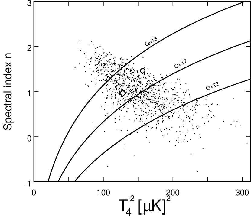
Figure 3: Scatter plot showing fitted values for the hexadecupole power and the spectral index $n$ using $3\leq\ell\leq 19$ for 1000 out of 4000 Monte Carlo skies calculated with ${{\langle Q_{RMS}^{2}\rangle^{0.5}}}=17\;{{\rm\mu K}}$ and $n=1$. The big circle is fit to the power spectrum of the 2 year 53+90 GHz maps, the big diamond is the fit to the mean of the Monte Carlo’s, and the dots are the Monte Carlo’s. The curves show combinations of $n$ and $T_{4}^{2}$ that give $Q=13,17\;\&\;22\;{{\rm\mu K}}$ (from top to bottom).

Seljak & Bertschinger (1993) have applied this method to the correlation function of the DMR maps. This method has the interesting property that if the observed power spectrum matches the model exactly then the fitted value of $Q$ is significantly less than the true value. At the minimum of $\chi^{2}$, which is $\chi^{2}=0$ in this case, there is still a large slope in $-2\ln(L)$ because of the rapid variation of $\ln(\det(C))$ with $Q$. Figure 3 shows this effect: the diamond symbol shows the values of the amplitude and $n$ obtained by minimizing $-2\ln(L)$ when the observed power spectrum is the mean of 4000 Monte Carlo’s with $n=1$ and $Q=17\;{{\rm\mu K}}$. It is clearly biased toward low amplitude when compared to the dots, which show fits to the individual power spectra from the 4000 Monte Carlo’s. The big circle shows the results of minimizing $-2\ln(L)$ for the real sky power spectrum from the 53+90 map with 2 years of data.

The maximum likelihood technique gives an asymptotically unbiased determination of the amplitude $Q$ and index $n$, but only as the observed solid angle goes to infinity. Since we are limited to about 8 sr of sky, asymptotically unbiased means biased in practice. In addition, the use of a Gaussian approximation for the likelihood of our quadratic statistics can introduce additional errors. We use our Monte Carlo simulations to calibrate our statistical methods to avoid biased final answers. If we maximize $L$ using the simplex method we find that the maximum likelihood index is biased upward from the input $n$ used in the Monte Carlo’s by $\approx 0.1$. An alternative method based on finding the zero in the finite difference $L(Q,n+0.2)-L(Q,n-0.2)$ gave a much smaller bias but sometimes failed to converge for power spectra that were not well fit by a power law.

The cross power spectrum of the real sky based on the (53A+90A)$\times$(53B+90B) maps is best fit in the range $3\leq\ell\leq 19$ by an $n=1.55$ model when we use the simplex method to maximize the likelihood. The improvement in $2\ln(L)$ between the fit with $n$ forced to be 1 and the $n=1.55$ model is 2.5, which corresponds to $1.6\;\sigma$. However, 14% of the Monte Carlo simulations made with $n_{in}=1$ and the maximum likelihood amplitude for $n=1$ give fitted values of $n$ that are larger than 1.55, so this deviation from a Harrison-Zeldovich spectrum is really only a “1.06 $\sigma$” deviation. Similarly, 54% of simulations made with $n_{in}=1.5$ and the maximum likelihood amplitude for $n=1.5$ had fitted indices higher than $1.55$, indicating that $n_{in}=1.5$ is actually too high by $0.10\,\sigma$. Using the same procedure we find that $n_{in}=0.5$ is $2.07\,\sigma$ low, $n_{in}=2$ is $1.41\,\sigma$ high, and $n_{in}=2.5$ is $2.81\,\sigma$ high. Interpolating to find values of $n_{in}$ that deviate by -1, 0 and +1 $\sigma$ defines our quoted limits on the spectral index for $3\leq\ell\leq 19$: $n={{1.46^{+0.39}_{-0.44}}}$.

With 4 years of data these limits will improve to $\Delta n\approx{}^{+0.32}_{-0.35}$ for the 53+90 maps if we assume that the maximum likelihood $n$ remains the same.

While waiting for this paper to be refereed, new computing facilities allowed us to increase $\ell_{max}$ to 30. The increased power at $20\leq\ell\leq 30$ expected for $n_{in}\approx 1.5$ is not seen in the real maps, so the fitted values of $n$ go down. Over the $3\leq\ell\leq 30$ range the fits to the cross power spectra are $n=1.32^{+0.39}_{-0.45}$ for (53A+90A)$\times$(53B+90B), $n=1.22^{+0.42}_{-0.46}$ for (53A+53B)$\times$(90A+90B), and $n=1.20^{+0.42}_{-0.46}$ for (53A+90B)$\times$(53B+90A). These values have all been de-biased using the Monte Carlo simulations as discussed above. Each of these fits involves 4 of the 6 possible cross spectra among the 53A, 53B, 90A and 90B maps. Averaging these three cross spectra gives us all of the 6 possible cross spectra. The signal-to-noise ratio improvement from using 6 instead of 4 cross products is quite modest, however, and is equivalent to a 22% increase in integration time. Thus the adopted range for the spectral index is $n={{1.25^{+0.4}_{-0.45}}}$.

The spectral index from the NG maps is $n={1.41^{+0.75}_{-1.17}}$, where the large uncertainty is caused by the increased noise in the NG maps. The galaxy removal process subtracts the relatively noisy 31 GHz channels of the DMR from a weighted sum of the quieter 53 and 90 GHz channels, and then rescales the result to allow for the partial cancellation of the cosmic $\Delta T$ by the subtraction. Both the subtraction and the rescaling increase the noise, and the overall process effectively doubles the radiometer noise.

The difference between the $n={1.22^{+0.42}_{-0.46}}$ reported here for $53\times 90$ and the $n=1.15$ reported by Smoot et al. (1992) is partly caused by the use of the real beam in this paper instead of the Gaussian beam approximation used by Smoot et al.. The ratio of $G_{10}/G_{4}$ from Wright et al. (1994) for the real beam to the same quantity for the Gaussian approximation is 0.92, and to compensate for the greater suppression of $\ell=10$ by the real beam the fitting procedure increases $n$ by 0.2. This increase has been partly compensated by a decrease of $n$ when going from the 1 year to the 2 year maps. The de-biased fit to the 1 year (53A+90A)$\times$(53B+90B) cross-power spectrum for $3\leq\ell\leq 30$ is $n=1.69^{+0.45}_{-0.52}$.

Bennett et al. (1994), using the real DMR beam instead of the Gaussian approximation, find that the maximum of the likelihood $L(Q,n)$ occurs at $Q=12.4\;{{\rm\mu K}},n=1.59$ from an analysis of the cross-correlation function of the 2 year $53\times 90$ GHz maps. This analysis included the quadrupole, and the low observed quadrupole leads to increased values of $n$ when it is included in the fit. A no quadrupole fit gives the maximum likelihood at $n=1.21^{+0.60}_{-0.55}$.

Smoot et al. (1994) give estimates of the spectral index $n$ derived from the variation with smoothing angle of the moments of the DMR maps, and of the genus of the DMR maps. The determination from moments is primarily based on the second moment, and the variation of the second moment with smoothing angle is equivalent to the power spectrum. This moment method gives $n=1.7^{+0.3}_{-0.6}$ when applied to the first year maps, which is quite consistent with the power spectrum of the first year maps. The genus method also gives $n=1.7$ but $n=1$ does not give a significantly worse fit.

Górski et al. (1994) examine linear statistics that are similar to $\langle G_{\ell m}T\rangle$. These have the major advantage that their distribution is exactly Gaussian, and thus the Gaussian form for the likelihood in Equation 17 is exact. The linear statistics used by Górski et al. define a position in a 961 dimensional space (for $\ell\leq 30$) which is hard to visualize, but using the exact Gaussian likelihood function for $3\leq\ell\leq 30$, Górski et al. (1994) find the maximum of $L(Q,n)$ occurs at $n=1.02$ for the combined 2 year 53 GHz plus 90 GHz map. Note that the $3\leq\ell\leq 30$ fits in this paper still include the small effect of the quadrupole on higher $\ell$’s due to the off-diagonal elements in the response matrix, while those in Górski et al. (1994) are completely independent of the quadrupole. If Equation 5 is modified to also subtract quadrupole terms from the $G_{\ell m}$’s, a different modified Hauser-Peebles power spectrum is obtained which is much more similar to the $\ell=3-30$ analysis of Górski et al. (1994). In this variant the mean power in $T_{4}^{2}$ for $n=1$ Monte Carlo skies goes down by 31% while $T_{4}^{2}$ for the real sky goes up by 16%, leading to a higher $\ell=4$ point that balances the high $\ell=14-19$ bin and reproduces the Górski et al. spectral index $n=1.0$. Also note that Górski et al. (1994) use a known shape and amplitude for the noise power, computed from the covariance matrix of the map, which allows them to use the “auto-power spectra”, while this paper just assumes that the A and B noises are uncorrelated and can only use cross-power spectra.

Table 4 summarizes these results and includes model-dependent comparisons of COBE data to smaller-scale data. The apparent large-scale index we have used above is denoted $n_{app}$, while the model-corrected primordial spectral index is $n_{pri}$.

Maximum likelihood fits for $Q$ with $n$ forced to be 1 over the $3\leq\ell\leq 30$ range give new determinations of the power spectrum amplitude: $Q=20.2\pm 1.8,\;19.2\pm 1.3$ and $15.6\pm 2.1\;{{\rm\mu K}}$ for the 53, 53+90 and NG maps. Comparing fits forced to $n=0.5$ and $n=1.5$ allows a determination of the effective wavenumber for these amplitudes: $\ell_{eff}=6.1$, 6.8 and 4.2 respectively. The amplitudes for the 53 and 53+90 maps are higher than the 17 ${\rm\mu K}$ reported earlier because the maximum likelihood fit has emphasized the higher $\ell$’s in determining the best fit since they have smaller cosmic variance, and shifting to higher $\ell$’s gives a higher amplitude because the best fit value of $n$ is greater than 1. The values from the NG maps are statistically consistent with the 53+90 maps, but the possibility of a galactic contribution to $Q$ and $n$ is much reduced with the NG map. The maps are actually more similar than the 26% spread in best fit $n=1$ amplitudes would suggest: the simpler $\sigma(10^{\circ})$ statistic computed using DMRSMUTH (see Wright et al. 1994) in $|b|>30^{\circ}$ is 31.9, 32.6 and 31.4 ${\rm\mu K}$ for the 53, 53+90 and NG maps respectively, a spread of only 4%; while the GET_SKY_RMS program in $|b|>20^{\circ}$ gives $\sigma(10^{\circ})=31.3$, 29.1 and 30.7 ${\rm\mu K}$, a spread of only 7%. Thus most of the difference in the best fit amplitudes is caused by the shift of the weights to higher $\ell$’s.

6 Comparison with Degree Scale Experiments

Several groups have reported statistically significant signals from $\Delta T$ experiments with beam sizes and chopper throws close to 1^∘. These results are usually reported as limits on the amplitude of a Gaussian correlation function,

$$C_{g}(\theta)=C_{g}(0)\exp(-0.5\theta^{2}/\theta_{c}^{2}).$$ (18)

We have calculated the conversion from the reported limits on Gaussian $C_{g}(0)$ to limits on power law power spectra as follows: first, given the size of a Gaussian approximation to the experiment beam, $\sigma_{B}=$FWHM$/\sqrt{8\ln 2}$, find the beam smoothed Gaussian correlation function:

$$C_{g,sm}(\theta)=C_{g}(0){{\theta_{c}^{2}}\over{\theta_{c}^{2}+2\sigma_{B}^{2}}}\exp[-0.5\theta^{2}/(\theta_{c}^{2}+2\sigma_{B}^{2})].$$ (19)

Then the single subtracted, double subtracted, triple subtracted (Python) or square pattern $({}^{+}_{-}{}^{-}_{+})$ double subtracted (WD2) temperature difference is found from

$${\rm var}(\Delta T_{SS}) = 2(C_{g,sm}(0)-C_{g,sm}(\theta))$$

$${\rm var}(\Delta T_{DS}) = 1.5C_{g,sm}(0)-2C_{g,sm}(\theta)+0.5C_{g,sm}(2\theta)$$

$${\rm var}(\Delta T_{TS}) = 1.25C_{g,sm}(0)-1.875C_{g,sm}(\theta)+0.75C_{g,sm}(2\theta)-0.125C_{g,sm}(3\theta)$$

$${\rm var}(\Delta T_{SQ}) = C_{g,sm}(0)-2C_{g,sm}(\theta)+C_{g,sm}(\sqrt{2}\theta)$$ (20)

where $\theta$ is the chopper throw. The same temperature differences are then estimated for power law power spectra with $Q=17\;{{\rm\mu K}}$ and $n=0.5,1,$ and 1.5 using the expression for the beam smoothed power law correlation function

$$C_{n,sm}(\theta) = Q^{2}{{\Gamma[(9-n)/2]}\over{\Gamma[(3+n)/2]}}$$ (21)

$$\times \sum_{\ell=2}^{\infty}{{(2\ell+1)}\over{5}}P_{\ell}(\cos\theta)\exp[-\ell(\ell+1)\sigma_{B}^{2}]{{\Gamma[\ell+(n-1)/2]}\over{\Gamma[\ell+(5-n)/2]}}.$$

With $Q$ held fixed, we can define the effective spherical harmonic order for a given experiment using

$$\ell_{eff}=2\times{{{\rm var}(\Delta T[n=1.5])}\over{{\rm var}(\Delta T[n=0.5]}}$$ (22)

where ${\rm var}(\Delta T)$ is one of the four expressions in Equation 20 with $C_{g,sm}$ replaced by $C_{n,sm}$ and the choice of which expression for ${\rm var}(\Delta T)$ to use depends on the chopping strategy used in each experiment. The ratio of the observed ${\rm var}(\Delta T)$ derived from $C_{g,sm}$ in Equation 20 to ${\rm var}(\Delta T[n=1])$ with $Q=17\;{{\rm\mu K}}$ then defines the $y$-axis coordinate in Figure 4, while $\ell_{eff}$ gives the $x$-axis coordinate.

Ganga et al. (1993, 1994) have have estimated the power spectral parameters $Q$ and $n$ using data from the Far Infra-Red Survey (FIRS), a balloon-borne survey experiment with a $3.8^{\circ}$ beam. They obtain $n=1.0^{+1.1}_{-1.0}$ which is consistent with the value in this paper. From the slope of their likelihood contours in the $Q-n$ plane, we derive an $\ell_{eff}=6.6$ for their $n=1$ amplitude determination, giving the FIRS point on Figure 4.

7 Conclusions

The Hauser-Peebles method of analyzing angular power spectra has been applied to the DMR maps. While the best fit to the observed power spectrum has $n={{1.25^{+0.4}_{-0.45}}}$, this deviation from the $n=1$ case is not statistically significant. To obtain a more accurate determination of $n$ we need to compare the COBE DMR amplitude with ground-based and balloon-based experiments at smaller angular scales, which are sensitive to higher $\ell$’s than COBE.

The ULISSE and Tenerife experiments (Watson et al. 1992) with beam sizes near $6^{\circ}$ and chopper throws of $6-8^{\circ}$ give upper limits in the $\ell_{eff}\approx 15$ range which support $n<1.5$. The new Tenerife results (Hancock et al. 1994) at the same angular scale as Watson et al. give a central value that is slightly above the earlier upper limit. Both are plotted in Figure 4.

The calculations of Kamionkowski & Spergel (1994) suggest that for open Universes with $\Omega\approx 0.1$ the power at low $\ell$’s will be depressed relative to the $n=1$ flat Universe prediction. This prediction is consistent with the data presented here, but fluctuations due to cosmic variance at low $\ell$’s are as large as the difference between the open Universe model and the scale-invariant flat Universe $n=1$ model.

The string model prediction given by Bennett, Stebbins & Boucher (1992b) also has lower power at small $\ell$’s, and is thus consistent with the COBE angular power spectrum, but a cutoff at higher $\ell$ is needed. Reionization of the Universe at redshift $z$ will hide structures on scales smaller than $60^{\circ}/\sqrt{1+z}$ and provide the needed cutoff, but $z{{}_{>}\atop{}^{\sim}}100$ is required to have a substantial optical depth with the baryon abundance derived from Big Bang nucleosynthesis (Walker et al. 1991). But reionization will not “smear out” the edges produced by strings seen at smaller redshifts. Thus, unlike most scientific models which can only be falsified, the string model can be verified by finding “the edge”, which will remain infinitely sharp even with reionization. The sharp edges in the $\Delta T$ maps produced by nearby strings limits the slope of the cutoff to $\ell^{-1}$ relative to an $n=1$ spectrum. Graham et al. (1994) find that the SP91 data is significantly non-Gaussian, which suggests that an edge may have been found. If true, this would increase the discrepancy among the degree-scale experiments, since the presence of an edge would increase the variance, but SP91 has the smallest variance of the four degree-scale experiments.

This expected increase in the variance due to non-Gaussian features is clearly present in the 20 GHz OVRO and RING experiments which have the same angular scale. The RING experiment covered a larger region, and was contaminated by discrete sources whose existence was verified by the VLA. The 170 GHz MSAM experiment also saw what appeared to be discrete sources, and these were not included in the analysis. There is no sensitive, higher angular resolution telescope to verify that the large deflections seen by MSAM are indeed point sources. Thus it is possible that the large deflections are true cosmic $\Delta T$’s. The open circles above the MSAM data points in Figure 4 show the increased power that results if these data are not excluded in the analysis.

The bulk flow data of Bertschinger et al. (1990) (at $\ell_{eff}\approx 10^{2}$) require $n\approx 1$ to agree with COBE (Wright et al. 1992), while the larger bulk flow on larger scales seen by Lauer & Postman (1992) requires $n\approx 2.9$ to agree with COBE, if we assume that the reported bulk flow represents the RMS velocity on this scale.

The experiments at $\approx 1^{\circ}$ scale offer the possibility of a better determination of the primordial power spectrum index $n$, but the model-dependent effects of the wing of the Doppler peak at $\ell\approx 200$ must be allowed for. Even in the large angle region $\ell<30$ small model-dependent corrections must be made. In Figure 4, the upper Cold Dark Matter (CDM) curve has a primordial spectral index $n_{pri}=0.96$, but an apparent index $n_{app}$ = 1.1. Since the spectral index ${1.25^{+0.4}_{-0.45}}$ found in this paper is an apparent index, the COBE power spectrum is consistent with the prediction from inflation and CDM or Mixed Dark Matter models that $n_{app}\approx 1.1$. On the other hand, vacuum-dominated models such as the Holtzman (1989) model with $\Omega_{B}=0.02$, $h=1$, $\Omega_{CDM}=0.18$, and $\Omega_{vac}=0.8$ will give $n_{app}=0.9$ for $n_{pri}=1.0$ (Kofman & Starobinski 1985), which deviates by slightly less than $1\sigma$ from the COBE value. We have found the values of the primordial spectral index $n_{pri}$ that will connect the COBE NG amplitude and $\ell_{eff}$ found earlier with the degree-scale experiments using the scalar transfer function from Crittenden et al. (1993). We have ignored the tensor transfer function because the current accuracy in determining $n$ is not sufficient to fix the tensor to scalar ratio, and because the excess quadrupole predicted by the tensor transfer function is not seen in the COBE power spectrum. The South Pole experiment of Schuster et al. (1993) at $\ell\approx 44$ requires $n_{pri}\approx 0.48\pm 0.34$ to agree with COBE. The Saskatoon experiment of Wollack et al. (1993) at $\ell\approx 55$ requires $n_{pri}\approx 1.04\pm 0.29$ to agree with COBE. The PYTHON experiment of Dragovan et al. (1994) at $\ell\approx 71$ requires $n_{pri}\approx 1.58\pm 0.22$ to match COBE. The ARGO experiment of de Bernardis et al. (1994) at $\ell\approx 75$ requires $n_{pri}\approx 1.10\pm 0.16$ to match COBE. The weighted mean of these values is $n_{pri}=1.15\pm 0.11$. Unfortunately $\chi^{2}=8.0$ with 3 degrees of freedom when comparing these four values of $n_{pri}$ with this weighted mean, indicating that these four experiments are mutually inconsistent. If we allow for this discrepancy by scaling the error on $n_{pri}$, we get a value $n_{pri}=1.15\pm 0.2\pm 0.1$ from this comparison of COBE with the degree-scale experiments, where the second error bar is contribution of the uncertainty of the COBE NG amplitude to $n_{pri}$. Thus this comparison of COBE with degree-scale experiments gives a more precise value the primordial spectral index that is still consistent with inflation. With more data from COBE (4 years are recorded) the large angular scale amplitude will become more and more certain. The $\ell_{eff}$ associated with this amplitude will shift to larger values $\approx 10$. Reliable, consistent determinations of $\delta T$ on scales $\ell_{eff}\approx 50$ will be needed to compare with the large-scale $\Delta T$. With only two years of data, the COBE DMR large scale amplitude has relative errors that are two times smaller than the errors of the current degree-scale experiments. Thus the degree-scale experiments need to be extended to a sky coverage that is 10 times higher than their current coverage to match the expected COBE uncertainty with four years of data, or else achieve an equivalent increase in accuracy by reduced noise or systematic errors.

We gratefully acknowledge the many people who made this paper possible: the NASA Office of Space Sciences, the COBE flight operations team, and all of those who helped process and analyze the data. In particular we thank Tony Banday, Krys Górski, Gary Hinshaw, Charlie Lineweaver, Mike Hauser, Mike Janssen, Steve Meyer and Rai Weiss for useful comments on the manuscript.

Table 1:

$\ell$	$\ell_{eff}$	2 YR 53		2 YR 53+90		2 YR 53$\times$90		2 YR NG		1 YR 53+90
2	2.1	0.59	$\pm 0.47$	0.44	$\pm 0.61$	0.45	$\pm 0.58$	0.17	$\pm 0.49$	0.58	$\pm 0.42$
3	3.1	1.06	$\pm 0.52$	1.04	$\pm 0.60$	1.01	$\pm 0.56$	0.96	$\pm 0.56$	0.90	$\pm 0.50$
4	3.3	1.16	$\pm 0.45$	1.11	$\pm 0.52$	1.12	$\pm 0.48$	1.05	$\pm 0.52$	1.14	$\pm 0.46$
5-6	4.4	1.23	$\pm 0.40$	1.21	$\pm 0.40$	1.22	$\pm 0.36$	1.00	$\pm 0.54$	1.06	$\pm 0.42$
7-9	6.2	1.03	$\pm 0.43$	1.23	$\pm 0.37$	1.19	$\pm 0.33$	1.26	$\pm 0.63$	1.19	$\pm 0.46$
10-13	8.7	1.31	$\pm 0.58$	1.51	$\pm 0.44$	1.15	$\pm 0.41$	-0.22	$\pm 1.12$	1.41	$\pm 0.71$
14-19	10.7	2.61	$\pm 0.91$	1.60	$\pm 0.67$	1.69	$\pm 0.65$	1.90	$\pm 2.34$	2.34	$\pm 1.27$
20-30	11.8	3.26	$\pm 2.60$	-1.14	$\pm 1.98$	0.58	$\pm 1.94$	-2.54	$\pm 7.83$	-0.19	$\pm 3.98$

Table 2: Ratio of the binned power spectrum from Equation 9 to a $Q=17\;{{\rm\mu K}}$, $n=1$ model.

$\ell=$	2	3	4	5-6	7-9	10-13	14-19	20-30
2 yr NG	55	208	234	319	365	-45	251	-161
Best fit	202	159	170	272	286	229	167	85
Q=17,n=1	316	216	225	318	290	202	132	63
Noise only	1374	1	253	181	-42	-28	-12	-3
		1660	11	745	213	-1	238	311
Signal & Noise	24871		2164	669	30	133	171	-186
	364	14803		10865	2018	139	226	-1782
	3611	-166	13599		18437	2307	-28	-1230
	1717	3922	1214	29146		42218	5603	264
	828	1426	720	3907	33123		87028	10292
	2055	-187	384	1078	3798	53633		241805
	1128	776	-354	949	-241	7243	95862
	-351	-211	430	-2326	-1799	229	9420	245629

Table 3: Binned Hauser-Peebles power spectrum of the 2 year NG maps, the best fit $n=1.4$ model, the nominal $Q=17,n=1$ model, all in ${{\rm\mu K}}^{2}$; the upper triangle of the covariance matrix from noise-only Monte Carlo runs, and the lower triangle of the covariance matrix from the best fit Monte Carlo runs in ${{\rm\mu K}}^{4}$.

Method	COBE dataset	Q?	Result	Reference
Correlation function	1 year 53$\times$90	N	$n_{app}=1.15^{+0.45}_{-0.65}$	Smoot et al. (1992)
COBE:$\sigma_{8}$	1 year 53+90	N	$n_{pri}=1\pm 0.23$	Wright et al. (1992)
Genus vs. smoothing	1 year 53	Y	$n_{app}=1.7^{+1.3}_{-1.1}$	Smoot et al. (1994)
RMS vs. smoothing	1 year 53	Y	$n_{app}=1.7^{+0.3}_{-0.6}$	Smoot et al. (1994)
Correlation function	2 year 53$\times$90	Y	$n_{app}=1.59^{+0.49}_{-0.55}$	Bennett et al. (1994)
Correlation function	2 year 53$\times$90	N	$n_{app}=1.21^{+0.60}_{-0.55}$	Bennett et al. (1994)
COBE : $1^{\circ}$ scale	2 year NG	N	$n_{pri}=1.15\pm 0.2$	this paper
Cross power spectrum	1 year (53A+90A)$\times$(53B+90B)	N	$n_{app}=1.69^{+0.45}_{-0.52}$	this paper
Cross power spectrum	2 year 53A$\times$53B	N	$n_{app}=1.41^{+0.75}_{-1.17}$	this paper
Cross power spectrum	2 year 53$\times$90	N	$n_{app}=1.22^{+0.42}_{-0.46}$	this paper
Cross power spectrum	2 year (53A+90A)$\times$(53B+90B)	N	$n_{app}=1.32^{+0.39}_{-0.45}$	this paper
Cross power spectrum	2 year (53A+90B)$\times$(53B+90A)	N	$n_{app}=1.20^{+0.42}_{-0.46}$	this paper
Cross power spectrum	2 year NGA$\times$NGB	N	$n_{app}=1.41^{+0.75}_{-1.17}$	this paper
Orthonormal functions	2 year 53+90	N	$n_{app}=1.02\pm 0.4$	Górski et al. (1994)

Table 4: Spectral index determinations

Figure 1: Power spectrum of the 2 year 53+90 DMR maps (points) compared to the mean $\pm 1\sigma$ range of Monte Carlo spectra computed for Harrison-Zeldovich skies with an expected Q = 17 $\mu$K. The lower band is the $\pm 1\sigma$ range for noise only Monte Carlos. The lines show the mean power spectra for Monte Carlo’s with $n=-0.5,0,0.5,1,1.5,2\;\&\;2.5$ all normalized to have the same input $\ell=4$ amplitude as the Q = 17 H-Z case.

Figure 2: Effective spherical harmonic index $\ell_{eff}$ vs $\ell$ for the $T_{\ell}^{2}$ statistics with a galactic plane cut of $|b|>19.5^{\circ}$ (solid curve and points for the binned statistics), and with no galactic plane cut (dashed curve). The dotted curve shows $\ell_{eff}=\ell$.

Figure 4: Power spectra normalized to the mean of 17 $\mu$K Harrison-Zeldovich Monte Carlo skies. COBE data points from the 2 year NG DMR maps. Models shown as thin curves: $n=1$, $Q=17$ ${\rm\mu K}$ is the horizontal line, the best fit $n=1.4$ power law is the slanted line, & tilted CDM including the effects of gravitational waves with the long dashed curve showing $n=0.96$ (predicted by $\phi^{4}$ chaotic inflation), and the short dashed curve showing $n=0.85$ where the tensor and scalar quadrupoles are equal (Crittenden et al. 1993). Points with “bent” ends on their error bars are from other experiments: FIRS (Ganga et al. 1993), (from left to right) ULISSE (de Bernardis et al. 1992), Tenerife (Watson et al. 1992 and Hancock et al. 1994), the South Pole (Schuster et al. 1993), Saskatoon (Wollack et al.1993), the Python experiment (Dragovan et al. 1994), ARGO (de Bernardis et al. 1994), MSAM single subtracted (Cheng et al. 1994), MAX (Gunderson et al. (1993) and Meinhold et al. (1993)), MSAM double subtracted, White dish second harmonic (Tucker et al. 1993), OVRO (Readhead et al. 1989), OVRO RING (Myers et al. 1993), and the Australia Telescope (Subrahmayan et al. 1993). The open circles above the MSAM points show the effects of not removing sources.

References

- (1) Bardeen, J. M., Steinhardt, P. J. & Turner, M. S. 1983, Phys. Rev. D, 28, 679-693.
- (2) Bennett, C. L. et al. 1992a, ApJL, 396, L7.
- (3)
- (4) Bennett, C. L. et al. 1994, submitted to the ApJ.
- (5) Bennett, D. P., Stebbins, A. & Bouchet, F. R. 1992b, ApJL, 399, L5-L8.
- (6) Bertschinger, E., Dekel, A., Faber, S. M., Dressler, A. & Burstein, D. 1990, ApJ, 364, 370-395.
- (7) Bond, J. R. & Efstathiou, G. 1987, M.N.R.A.S, 226, 655-687.
- (8) Cheng, E. S., Cottingham, D. A., Fixsen, D. J., Inman, C. A., Kowitt, M. S., Meyer, S. S., Page, L. A., Puchalla, J. L. & Silverberg, R. F. 1994, ApJL, 422, L37-L40.
- (9) Crittenden, R., Bond, J. R., Davis, R. L., Efstathiou, G. & Steinhardt, P. J. 1993, PRL, 71, 324-327.
- (10) de Bernardis, P., Masi, S., Melchiorri, F., Melchiorri, B. & Vittorio, N. 1992, ApJ, 396, L57-L60.
- (11) de Bernardis, P., Aquilini, E., Boscaleri, A., De Petris, M., D’Andreta, G., Gervasi, M., Kreysa, E., Martinis, L., Masi, S., Palumbo, P. & Scaramuzzi, F. 1994, ApJL, 422, L33-L36.
- (12)
- (13) Dragovan, M., Ruhl, J., Novak, G., Platt, S. R., Crone, B., Peterson, J. B. & Pernic, R. 1994, submitted to the ApJ.
- (14) Ganga, K., Cheng, E., Meyer, S. & Page, L. 1993, ApJL, 410, L57.
- (15)
- (16) Ganga, K., Page, L., Cheng E., & Meyer, S. 1994, submitted to the ApJL.
- (17)
- (18) Graham, P., Turok, N., Lubin, P. M. & Schuster, J. A. 1994, submitted to the ApJ.
- (19)
- (20) Górski, K. M., Hinshaw, G., Banday, A. J., Bennett, C. L., Wright, E. L., Kogut, A., Smoot, G. F. & Lubin, P. 1994, submitted to the ApJL.
- (21) Guth, A. 1981, Phys. Rev. D, 23, 347.
- (22) Hancock, S., Davies, R. D., Lasenby, A. N., Gutierrez de la Cruz, C. M., Watson, R. A., Rebolo, R. & Beckman, J. E. 1994, Nature, 367, 333-337.
- (23) Harrison, E. R. 1970, Phys Rev D, 1, 2726-2730.
- (24) Hauser, M. G. & Peebles, P. J. E. 1973, ApJ, 185, 757-785.
- (25)
- (26) Hinshaw, G., Kogut, A., Górski, K. M., Banday, A. J., Bennett, C. L., Lineweaver, C., Lubin, P., Smoot, G. F. & Wright, E. L. 1994, submitted to the ApJ.
- (27) Holtzman, J. A. 1989, ApJSupp, 71, 1.
- (28)
- (29) Kamionkowski, M. & Spergel, D. 1994, submitted to the ApJ.
- (30) Kofman, L. A. & Starobinski, A. A. 1985, Soviet Astronomy Letters, 11, 271-274.
- (31) Lauer, T. & Postman, M. 1992, BAAS, 24, 1264.
- (32)
- (33) Lineweaver, C. H., Smoot, G. F., Bennett, C. L., Wright, E. L., Tenorio, L., Kogut, A., Keegstra, P. B., Hinshaw, G. & Banday, A. J. 1994, submitted to the ApJ.
- (34) Meinhold, P., Clapp, A., Devlin, M., Fischer, M., Gundersen, J., Holmes, W., Lange, A., Lubin, P., Richards, P. & Smoot, G. 1993, ApJL, 409, L1-L4.
- (35) Myers, S. T., Readhead, A. C. S., & Lawrence, C. R. 1993, ApJ, 405, 8-29.
- (36) Peebles, P. J. E. 1973, ApJ, 185, 413-440.
- (37) Peebles, P. J. E. & Yu, J. T. 1970, ApJ, 162, 815-836.
- (38) Readhead, A. C. S., Lawrence, C. R., Myers, S. T., Sargent, W. L. W., Hardebeck, H. E. & Moffet, A. T. 1989, Ap. J., 346, 566.
- (39) Schuster, J., Gaier, T., Gundersen, J., Meinhold, P., Koch, T., Seiffert, M., Wuensche, C. & Lubin P. 1993, ApJL, 412, L47-L50.
- (40)
- (41) Scott, D., Srednicki, M. & White, M. 1994, submitted to the ApJL.
- (42) Seljak, U. & Bertschinger, E. 1993, ApJL, 417, L9-L12.
- (43) Smoot, G. et al. 1992, ApJL, 396, L1.
- (44)
- (45) Smoot, G. et al. 1994, submitted to the ApJ.
- (46) Subrahmayan, R., Ekers, R. D., Sinclair, M. & Silk, J. 1993, MNRAS, 263, 416-424.
- (47) Tucker, G. S., Griffin, G. S., Nguyen, H. T. & J. B. Peterson, 1993, ApJL, 419, L45.
- (48) Walker, T. P., Steigman, G., Schramm, D. N., Olive, K. A. & Kang, H-S. 1991, ApJ, 376, 51-69.
- (49) Watson, R. A., Gutierrez de la Cruz, C. M., Davies, R. D., Lasenby, A. N., Rebolo, R., Beckman, J. E. & Hancock, S. 1992, Nature, 357, 660-665.
- (50) Wollack, E. J., Jarosik, N. C., Netterfield, C. B., Page, L. A. & Wilkinson, D. T. 1993, ApJL, 419, L49.
- (51) Wright, E. L. et al. 1992, ApJL, 396, L13.
- (52) Wright, E. L. 1993, Annals of the New York Academy of Sciences, 688, 836-838.
- (53) Wright, E. L., Smoot, G. F., Kogut, A., Hinshaw, G., Tenorio, L., Lineweaver, C., Bennett, C. L. & Lubin, P. M. 1994, ApJ, 420, 1.
- (54) Zeldovich, Ya. B. 1972, MNRAS, 160, 1p.
- (55)