= 0.9 in

SU–ITP–93–29

IEM–FT–77/93

astro-ph/9312039

16 December 1993

Fluctuations of the Gravitational Constant

in the Inflationary Brans–Dicke Cosmology

Juan García–Bellido,

Andrei Linde, Department of Physics, Stanford University, Stanford, CA 94305-4060, USA
Dmitri Linde California Institute of Technology, Pasadena, CA 91125, USA

Abstract

According to the Brans–Dicke theory, the value of the gravitational constant $G$ which we measure at present is determined by the value of the Brans–Dicke scalar field $\phi$ at the end of inflation. However, due to quantum fluctuations of the scalar fields produced during inflation, the gravitational constant $G(\phi)$ may take different values in different exponentially large parts of the Universe. We investigate the probability distribution $P_{p}$ to find a domain of a given volume with a given value of the gravitational constant $G$ at a given time. The investigation is performed for a wide class of effective potentials of the scalar field $\sigma$ which drives inflation, and with two different time parametrizations. Our work is based on the analytical study of the diffusion equations for $P_{p}$, as well as on the computer simulation of stochastic processes in the inflationary Universe. We have found that in some inflationary models the probability distribution $P_{p}$ rapidly approaches a stationary regime. The shape of the distribution depends, however, on the choice of the time parametrization. In some other models the distribution $P_{p}$ is not stationary. An interpretation of our results and of all ambiguities involved is outlined, and a possible role of anthropic considerations in determination of the gravitational constant is discussed.

1 Introduction

One of the most amazing properties of inflationary cosmology is the process of self-reproduction of inflationary domains of the Universe (for a review see [1]). This process exists in many versions of inflationary universe scenario, including old inflation [2], new inflation [3, 4], chaotic inflation [5] and extended inflation [6]. Self-reproduction of inflationary domains implies that there is no end of the evolution of the Universe. This process divides the Universe into many exponentially large domains with all types of symmetry breaking and with all types of compactification of space-time compatible with inflation.

The best way to describe the global structure of the Universe in this scenario is provided by the stochastic approach to inflation. The original version of this approach [7] was based on the investigation of the distribution of probability $P_{c}(\phi,t)$ to find a given field $\phi$ at a given time at a given point. This approach was not well suited for the investigation of the process of self-reproduction of the Universe. A more adequate approach is based on investigation of the distribution of probability $P_{p}(\phi,t)$ to find a given field $\phi$ at a given time in a given physical volume [5, 8, 9].

The most detailed study of the distribution $P_{p}$ was performed recently in [10], where it was shown that in many inflationary models including the models with the effective potentials $\phi^{n}$ and $e^{\alpha\phi}$ this probability distribution rapidly approaches a stationary regime. This means that if one takes a section of the Universe at a given time $t$ and calculates the relative fraction of domains of the Universe with given properties (with given density, with given values of various scalar fields, etc.), the result will not depend on the time $t$, both during inflation and after it.

This result represents a major deviation of inflationary cosmology from the standard Big Bang paradigm. A lot of work is still needed to verify this result and to obtain its consistent interpretation in the context of quantum cosmology. One should also study how our methods work in the context of more complicated models, including several different scalar fields [11, 12, 10].

A natural idea would be to apply our methods to extended inflation scenario [13], which is a hybrid of the Brans–Dicke theory and old inflation. In this scenario one has two scalar fields: the Brans–Dicke field $\phi$ and the inflaton field $\sigma$. However, during extended inflation only the former evolves in time, which reduces the problem to the one we have studied already. Moreover, the value of the scalar field $\phi$ after inflation in this theory typically is determined not by the stochastic dynamics during inflation, but either by the position of a pole of a non-minimal kinetic term of the field $\phi$ or by the effective potential of this field which should be introduced into the theory in order to make it consistent with observational data [14].

In this paper we will consider theories of another type, which are hybrids of the Brans–Dicke theory with new [15, 16] or chaotic inflation [17]. In these models, especially in the chaotic inflation model of ref. [17], simultaneous stochastic evolution of the fields $\phi$ and $\sigma$ is very nontrivial. One of the most interesting consequences of this evolution is the division of the Universe after inflation into exponentially large regions with different values of the gravitational constant in each of them. Indeed, the gravitational constant $G$ in the Brans–Dicke theory is a function of the field $\phi$,

$$G=M_{\rm p}^{-2}(\phi)={\omega\over 2\pi\phi^{2}}\ ,$$ (1)

where $\omega$ is the Brans–Dicke parameter, $\omega>500$ [18, 19]. The value of the scalar field $\phi$ practically does not change after inflation. Therefore, investigation of the distribution $P_{p}(\phi,t)$ gives us the fraction of the physical volume of the Universe where the gravitational constant $G$ has the effective value (1).

The stationary character of the probability distribution $P_{p}(\sigma)$ in the theory of one scalar field $\sigma$ in the standard general relativity theory is closely related to the existence of the Planck boundary $\sigma_{p}$, where the potential energy density $V(\sigma)$ becomes comparable with the Planck density $M_{\rm p}^{4}$. Typically the distribution $P_{p}(\sigma,t)$ rapidly moves towards large $\sigma$, for the reason that the volume of domains with large $V(\sigma)$ grows very fast. The distribution $P_{p}(\sigma,t)$ becomes stabilized as it approaches the Planck boundary, where, as it is argued in [10], the process of self-reproduction of inflationary domains is less efficient.

In the Brans–Dicke theory the situation is somewhat different. The Planck boundary is not a point, but a line $\phi_{p}(\sigma_{p})$, where

$$V(\sigma_{p})=M_{\rm p}^{4}(\phi_{p})={4\pi^{2}\over\omega^{2}}\phi_{p}^{4}\ .$$ (2)

Therefore, after the distribution $P_{p}(\sigma,\phi;t)$ approaches the Planck boundary, it can still move along this boundary. One may encounter three different possibilities:

1) The distribution $P_{p}(\sigma,\phi;t)$ never becomes stationary for any values of $\phi$ and $\sigma$. Nevertheless the properties of domains of inflationary universe filled by the fields $\phi$ and $\sigma$ do not depend on the time when these domains were formed. This is the most profound stationarity which is present in all inflationary models where the process of self-reproduction of inflationary domains is possible. In ref. [10] we called this property microstationarity, or local stationarity.

2) The distribution $P_{p}(\sigma,\phi;t)$ normalized over all possible values of $\phi$ and $\sigma$ gradually approaches a stationary regime. In ref. [10] we called this property macrostationarity, or global stationarity.

3) The maximum of the distribution $P_{p}(\sigma,\phi;t)$ runs away to infinitely large (or to infinitely small) values of $\phi$ and $\sigma$. As a result, the relative fraction of volume filled by any finite $\phi$ and $\sigma$ as compared with the total volume of the Universe decreases in time, which means that the global stationarity is absent. However, one may wish to exclude from consideration domains with infinitely large (or infinitely small) values of $\phi$ and $\sigma$ and concentrate on some finite part of space ($\phi,\sigma$) (for example, on those values of $\phi$ and $\sigma$ which are consistent with the existence of life as we know it). Then in some cases one may find out that the probability distribution $P_{p}(\sigma,\phi;t)$ normalized over this part of space ($\phi,\sigma$) (or the ratio $P_{p}(\sigma,\phi;t)\over P_{p}(\sigma_{0},\phi_{0},t)$) approaches a stationary regime. In this case we will speak of a runaway stationarity.

As we will see, all these possibilities may be realized in the inflationary Brans–Dicke cosmology, depending on the choice of the effective potential $V(\sigma)$.

There exists another important issue to be discussed in this paper. Even if the distribution $P_{p}(\sigma,\phi;t)$ does not depend on time, it may depend on the choice of possible time parametrizations [10]. As we will see, in the Brans–Dicke theory this dependence can be quite strong.

In Section 2 of this paper we describe chaotic inflation in the Brans–Dicke theory at the classical level, following ref. [17]. In Section 3 we derive the stochastic equations describing the evolution of quantum fluctuations of the scalar fields $\phi$ and $\sigma$ during inflation, as well as the origin of adiabatic energy density perturbations from these fluctuations. In Section 4 we describe the phenomenon of self-reproduction of the inflationary universe in the presence of both scalar fields as well as the stochastic approach to inflation in Brans–Dicke theory. We study the boundary conditions for $P_{p}$ in Section 5. These equations are extremely complicated, and it is not always possible to solve them analytically. Therefore we performed a computer simulation of the stochastic evolution of the scalar fields during inflation. We describe these numerical simulations and their results in Section 6. In Section 7 we analyze the case of a constant vacuum energy density, where runaway stationarity appears. For general increasing potentials $V(\sigma)$, the probability distribution in the physical frame will rapidly move to large values of $\sigma$, constituting what we called runaway solutions. These non–stationary solutions are described in Section 8. Imposing boundary conditions at large $\sigma$ or introducing steep potentials $V(\sigma)$ will give a stationary distribution, as described both numerically an analytically in Section 9. In Section 10 we derive the stochastic equations using a different time parametrization, where instead of the usual time $t$ we choose the time $\tau\sim\ln a(t)$ [7, 10]. The methods of computer simulations of stochastic evolution in time $\tau$ are different from the methods which we use in our simulations of the evolution in time $t$. We describe these methods and their results in Section 11. We compare the results obtained in different time parametrizations and make an attempt of their interpretation in Section 12.

As we already mentioned, under certain conditions the probability distribution $P_{p}$ is stationary, i.e. time-independent. This apparently gives us a possibility to calculate the position of the maximum of the distribution $P_{p}$ and thus predict the most probable value of the gravitational constant in the Universe. However, this idea involves some ambiguous speculations. The readers will find them in the Appendix.

2 Inflationary Brans–Dicke Cosmology

In this section we will describe the classical evolution of the inflaton field with a generic chaotic potential, in the context of the Jordan–Brans–Dicke theory of gravity,

$${\cal S}=\int d^{4}x\sqrt{-g}\left[{M_{\rm p}^{2}(\phi)\over 16\pi}R-{1\over 2}(\partial\phi)^{2}-{1\over 2}(\partial\sigma)^{2}-V(\sigma)\right]\ .$$ (3)

Here $M_{\rm p}^{2}(\phi)={2\pi\over\omega}\phi^{2}$,   $\phi^{2}/8\omega$ is the Brans–Dicke field, and $\sigma$ is the inflaton field. We will consider several different potentials, including $V(\sigma)\sim{m^{2}\over 2}\sigma^{2}$,  ${\lambda\over 4}\sigma^{4}$,  ${1\over 4\lambda}(m^{2}-\lambda\sigma^{2})^{2}$ and ${m^{2}\over 2}\sigma^{2}+{\lambda\over 4}\sigma^{4}\,\log{\sigma\over\sigma_{0}}$. The theory (3) looks similar to the extended inflation model [13]. The difference, which will be very important for us, is that in the extended inflation scenario inflation occurs at $\sigma=0$, whereas in our case inflation occurs during the slow rolling of the field $\sigma$ [17]. The complete equations of motion in a FRW Universe with scalar fields $\phi$ and $\sigma$ are

$$\begin{array}[]{c}{\displaystyle\left(D^{2}+\frac{1}{4\omega}R\right)\phi(t)=0}\ ,\\[8.53581pt] {\displaystyle D^{2}\sigma(t)=-\frac{\partial V}{\partial\sigma}}\ ,\\[8.53581pt] {\displaystyle H^{2}+\frac{\kappa}{a^{2}}=\frac{4\omega}{3\phi^{2}}\left({1\over 2}\dot{\phi}^{2}+{1\over 2}\dot{\sigma}^{2}+V(\sigma)\right)-2H\frac{\dot{\phi}}{\phi}}\ ,\end{array}$$ (4)

where $k=\pm 1,0$; $D^{2}\equiv\partial^{2}/\partial t^{2}+3H\partial/\partial t-k^{2}/a^{2}$, and $H=\dot{a}/a$. During inflation we can consistently use the slow roll–over approximations, $V^{\prime\prime}(\sigma),\ k^{2}/a^{2}\ll H^{2}$, $\ \ddot{\phi}\ll H\dot{\phi}\ll H^{2}\phi$, $\ {1\over 2}\dot{\sigma}^{2}+{1\over 2}\dot{\phi}^{2}\ll V(\sigma)$. The equations of motion (4) then simplify to

$$\begin{array}[]{c}{\displaystyle\dot{\phi}=\frac{\phi}{\omega}H\ ,\hskip 14.22636pt\hskip 14.22636pt\dot{\sigma}=-\frac{V^{\prime}(\sigma)}{3H}\ ,}\\[8.53581pt] {\displaystyle R=-12H^{2}\ ,\hskip 14.22636pt\hskip 14.22636ptH^{2}=\frac{4\omega}{3\phi^{2}}V(\sigma)}\ .\end{array}$$ (5)

We will be most interested in theories with $V(\sigma)=\frac{\lambda}{2n}\sigma^{2n}$, for which equations (5) reduce to

$$\begin{array}[]{c}{\displaystyle\dot{\phi}=\frac{2}{n}\left(\frac{n\lambda}{6\omega}\right)^{1/2}\sigma^{n}}\ ,\\[8.53581pt] {\displaystyle\dot{\sigma}=-\frac{\phi}{\sigma}\left(\frac{n\lambda}{6\omega}\right)^{1/2}\sigma^{n}}\ .\end{array}$$ (6)

It follows that in those theories $\ \phi$ and $\ \varphi\equiv\sqrt{2\over n}\ \sigma$ move along a circle of constant radius in the plane $(\varphi,\phi)$. We can parametrize the classical trajectory by polar coordinates $(\phi(t),\varphi(t))=(r\sin\theta(t),r\cos\theta(t))$ with constant $r$, and angular velocity

$$\dot{\theta}(t)=\left(\frac{\lambda}{3\omega}\right)^{1/2}\left(\frac{n}{2}\right)^{\frac{n-1}{2}}[r\cos\theta(t)]^{n-1}\ .$$ (7)

For $n=1$ we find solutions with a constant angular velocity

$$\begin{array}[]{rl}\phi(t)=&{\displaystyle r\ \sin\left(\theta_{o}+\frac{m}{\sqrt{3\omega}}t\right)}\ ,\\[8.53581pt] \sigma(t)=&{\displaystyle\frac{r}{\sqrt{2}}\ \cos\left(\theta_{o}+\frac{m}{\sqrt{3\omega}}t\right)}\ ,\\[11.38109pt] a(t)=&{\displaystyle a_{o}\ \left(\frac{\sin\left(\theta_{o}+{m\over\sqrt{3\omega}}t\right)}{\sin\theta_{o}}\right)^{\omega}}\ .\end{array}$$ (8)

Here $0<\theta_{o}<\pi/2$. These solutions in the interval $\theta_{o}{\sqrt{3\omega}\over m}<t\ll{\pi\sqrt{3\omega}\over 2m}$ correspond to the usual power–law behavior $a(t)\sim t^{\omega}$. For $n\geq 2$, the angular velocity decreases with time and the classical solutions are more complicated, but inflation is still power-law. These solutions are actually attractors of the complete equations of motion (4), for all $n$ [20].

We will now discuss initial and final conditions for the inflationary universe. In the chaotic inflation scenario, the most natural initial conditions for inflation are set at the Planck boundary, $V(\sigma_{p})=M_{\rm p}^{4}(\phi_{p})$, beyond which a classical space–time has no meaning and the energy gradient of the inhomogeneities produced during inflation becomes greater than the potential energy density, thus preventing inflation itself. The initial conditions for inflation are thus defined at the curve $\phi_{p}=\left(\frac{\omega}{2\pi}\right)^{1/2}\left({\lambda\over 2n}\right)^{1/4}\sigma_{p}^{n/2}$. On the other hand, inflation will end when the kinetic energy density of the scalar fields becomes comparable with the potential energy density, ${1\over 2}\dot{\phi}^{2}+{1\over 2}\dot{\sigma}^{2}\simeq V(\sigma)$ or $m^{2}=V^{\prime\prime}(\sigma)=H^{2}(\phi,\sigma)$. This condition corresponds to the end of inflation boundary $\sigma_{e}={n\over 2\sqrt{3\pi}}M_{\rm p}(\phi_{e})={n\over\sqrt{6\omega}}\phi_{e}$.

We will also consider an inflaton potential which leads to spontaneous symmetry breaking, $V(\sigma)={\lambda\over 4}\left(\sigma_{o}^{2}-\sigma^{2}\right)^{2}$, where $\sigma_{o}\equiv{m\over\sqrt{\lambda}}$. In this theory equations (5) are expressed as

$$\begin{array}[]{rl}\dot{\phi}=&{\displaystyle\left(\frac{\lambda}{3\omega}\right)^{1/2}|\sigma_{o}^{2}-\sigma^{2}|}\ ,\\[8.53581pt] \dot{\sigma}=&{\displaystyle\left(\frac{\lambda}{3\omega}\right)^{1/2}\phi\sigma\ \frac{|\sigma_{o}^{2}-\sigma^{2}|}{\sigma_{o}^{2}-\sigma^{2}}}\ .\end{array}$$ (9)

The fields move approximately along a circle centered at $\sigma=\sigma_{o}$, in clockwise direction if the initial condition is to the left of the minimum of the potential and in anticlockwise direction if it is to the right. In fact, for $\sigma\gg\sigma_{o}$ they will soon approach the asymptotic solution to (6) with $n=2$, while for $\sigma\ll\sigma_{o}$, we find the solution

$$\begin{array}[]{rl}\phi(t)=&{\displaystyle\frac{m^{2}}{\sqrt{3\omega\lambda}}\ t}\ ,\\[11.38109pt] \sigma(t)=&{\displaystyle\exp\left(\frac{m^{2}}{6\omega}t^{2}\right)}\ ,\\[8.53581pt] a(t)=&a_{0}\ t^{\omega}\ .\end{array}$$ (10)

Inflation will now occur in two disjoint sectors, either to the left or to the right of the minimum. The Planck boundary for initial conditions is again defined by $V(\sigma)=M_{\rm p}^{4}(\phi)$, while the end of inflation is given by the condition ${1\over 2}\dot{\sigma}^{2}\simeq V(\sigma)$. These two boundaries are defined by the curves

$$\begin{array}[]{rl}\phi_{p}=&{\displaystyle\left(\frac{\omega\sqrt{\lambda}}{4\pi}\right)^{1/2}|\sigma_{o}^{2}-\sigma_{p}^{2}|^{1/2}}\ ,\\[8.53581pt] \phi_{e}=&{\displaystyle\left(\frac{3\omega}{2}\right)^{1/2}{|\sigma_{o}^{2}-\sigma_{e}^{2}|\over\sigma_{e}}}\ .\end{array}$$ (11)

In the absence of any potential for $\phi$, the Brans–Dicke field remains almost constant after inflation, and therefore the Planck mass today is approximately given by its value at the end of inflation, $M_{\rm p}\simeq\sqrt{2\pi\over\omega}\ \phi_{e}\$. On the other hand, the total amount of inflation is approximately ${a_{e}\over a_{p}}\simeq\left({\phi_{e}\over\phi_{p}}\right)^{\omega}$.

The value of the Brans–Dicke parameter $\omega$ is bounded by post-Newtonian experiments [18] and primordial nucleosynthesis [19] to be very large, $\omega>500$, and therefore it is appropriate to use the approximation $\omega\gg 1$ in the following analysis.

3 Stochastic Methods

In this section we will describe the stochastic evolution of the scalar fields during inflation and the generation of adiabatic energy density fluctuations from quantum fluctuations of these fields.

3.1 Quantum Fluctuations of Scalar Fields

The classical scalar fields $\phi$ and $\sigma$ in de Sitter space are perturbed by their own quantum fluctuations, which are stretched beyond the horizon and act on the quasi–homogeneous background fields like a stochastic force. In order to calculate this effect we will coarse–grain over a horizon distance and split the scalar fields into long–wavelength classical background fields $\bar{\phi}(x)$ and $\bar{\sigma}(x)$ plus short–wavelength quantum fluctuations with physical momenta $k/a>H$,

$$\begin{array}[]{rl}\phi(\vec{x},t)=&{\displaystyle\bar{\phi}(\vec{x},t)+\int d^{3}k\ \theta(k-\varepsilon aH)\left[a_{k}u_{k}(x)+a^{\dagger}_{k}u^{\ast}_{k}(x)\right]}\ ,\\[8.53581pt] \sigma(\vec{x},t)=&{\displaystyle\bar{\sigma}(\vec{x},t)+\int d^{3}k^{\prime}\ \theta(k^{\prime}-\varepsilon aH)\left[b_{k^{\prime}}v_{k^{\prime}}(x)+b^{\dagger}_{k^{\prime}}v^{\ast}_{k^{\prime}}(x)\right]}\ ,\end{array}$$ (12)

where $\varepsilon$ is an arbitrary parameter that shifts the scale for coarse–graining [7]. The physical results turn out to be independent of the choice of $\varepsilon$. The quantum fluctuations are assumed to satisfy the following commutation relations

$$\begin{array}[]{c}[a_{k},a^{\dagger}_{k^{\prime}}]=[b_{k},b^{\dagger}_{k^{\prime}}]=\delta^{3}(\vec{k}-\vec{k}^{\prime})\ ,\ \ \ \ [a_{k},b^{\dagger}_{k^{\prime}}]=0\ {}.\par\end{array}$$ (13)

The exact solutions to the scalar fields’ equations (4) in de Sitter space with $V(\sigma)={1\over 2}m^{2}\sigma^{2}$ are given by [21]

$$\begin{array}[]{rl}u_{k}(x)=&{\displaystyle{e^{i\vec{k}\cdot\vec{x}}\over(2\pi)^{3/2}}\ {H\eta\over 2}\sqrt{\pi\eta}\ H_{\mu}^{(2)}(k\eta)\ ,\hskip 14.22636pt\hskip 14.22636pt\mu^{2}=\frac{9}{4}+\frac{3}{\omega}\simeq\frac{9}{4}}\ ,\\[11.38109pt] v_{k^{\prime}}(x)=&{\displaystyle{e^{i\vec{k^{\prime}}\cdot\vec{x}}\over(2\pi)^{3/2}}\ {H\eta\over 2}\sqrt{\pi\eta}\ H_{\nu}^{(2)}(k^{\prime}\eta)\ ,\hskip 14.22636pt\hskip 14.22636pt\nu^{2}=\frac{9}{4}-\frac{m^{2}}{H^{2}}\simeq\frac{9}{4}}\ ,\end{array}$$ (14)

where $\eta=-(aH)^{-1}$ is the conformal time, and $H^{(2)}_{3/2}(x)=-\sqrt{2\over\pi x}\exp(ix)\left(1+{i\over x}\right)$. The amplitude of the quantum fluctuations of $\phi$ and $\sigma$ can be computed as

$$\begin{array}[]{c}{\displaystyle\delta\phi=\left(4\pi k^{3}|u_{k}|^{2}\right)^{1/2}={H\over 2\pi}}\ ,\\[8.53581pt] {\displaystyle\delta\sigma=\left(4\pi k^{\prime 3}|v_{k^{\prime}}|^{2}\right)^{1/2}={H\over 2\pi}}\ ,\end{array}$$ (15)

which coincides with the Gibbons–Hawking temperature.

These quantum fluctuations then act as a stochastic force on the classical background fields. One could write the evolution of the coarse–grained fields in the form of Langevin equations

$$\begin{array}[]{c}{\displaystyle\frac{\partial\phi}{\partial t}=-\frac{M_{\rm p}^{2}(\phi)}{2\pi}\frac{\partial H}{\partial\phi}+\frac{H^{3/2}}{2\pi}\zeta(t)}\ ,\\[8.53581pt] {\displaystyle\frac{\partial\sigma}{\partial t}=-\frac{M_{\rm p}^{2}(\phi)}{4\pi}\frac{\partial H}{\partial\sigma}+\frac{H^{3/2}}{2\pi}\xi(t)}\ ,\end{array}$$ (16)

where $\zeta$ and $\xi$ behave like an effective white noise generated by quantum fluctuations, $\left\langle\zeta(t)\ \zeta(t^{\prime})\right\rangle\\ =\left\langle\xi(t)\ \xi(t^{\prime})\right\rangle=\delta(t-t^{\prime})$ and $\ \left\langle\zeta(t)\ \xi(t^{\prime})\right\rangle=0$, which leads to a Brownian motion of the classical scalar fields $\phi$ and $\sigma$, with a typical step (15).

We can alternatively describe the stochastic process in terms of the probability distribution $P_{c}(\sigma,\phi;t)$. This distribution describes the probability to find the fields $\phi$ and $\sigma$ at a given time $t$ in a given point. Equivalently, it describes the probability to find, at a given time $t$ in the domain with a given comoving (i.e. non-expanding) volume, the fields with mean values $\phi$ and $\sigma$. As it was shown by Starobinsky [7], this probability distribution satisfies the Fokker–Planck equation,

$$\begin{array}[]{rl}{\displaystyle\frac{\partial P_{c}}{\partial t}}=&{\displaystyle\frac{\partial}{\partial\sigma}\left(\frac{M_{\rm p}^{2}(\phi)}{4\pi}\frac{\partial H}{\partial\sigma}P_{c}+\frac{H^{3/2}}{8\pi^{2}}\frac{\partial(H^{3/2}P_{c})}{\partial\sigma}\right)}\\[8.53581pt] +&{\displaystyle\frac{\partial}{\partial\phi}\left(\frac{M_{\rm p}^{2}(\phi)}{2\pi}\frac{\partial H}{\partial\phi}P_{c}+\frac{H^{3/2}}{8\pi^{2}}\frac{\partial(H^{3/2}P_{c})}{\partial\phi}\right)\equiv-\frac{\partial J_{\sigma}}{\partial\sigma}-\frac{\partial J_{\phi}}{\partial\phi}}\ ,\end{array}$$ (17)

where we have chosen the Stratonovich version of stochastic processes. This equation can be interpreted as the continuity equation ${\displaystyle\ {\partial P_{c}\over\partial t}+\nabla\cdot J=0\ }$ associated with the conservation of probability. The first terms of each current correspond to the classical drift forces for the fields $\phi$ and $\sigma$ (6), while the second terms correspond to the quantum diffusion due to short–wavelength fluctuations (15).

One can then compute the field correlations during inflation with the help of this probability distribution, assuming that $H$ is approximately constant,

$$\begin{array}[]{rl}{\displaystyle\frac{\partial}{\partial t}\left\langle\phi^{p}\sigma^{q}\right\rangle=}&{\displaystyle\frac{H^{3}}{8\pi^{2}}p(p-1)\left\langle\phi^{p-2}\sigma^{q}\right\rangle+\frac{4p}{3H}\left\langle\phi^{p-2}\sigma^{q}V(\sigma)\right\rangle}\\[8.53581pt] +&{\displaystyle\frac{H^{3}}{8\pi^{2}}q(q-1)\left\langle\phi^{p}\sigma^{q-2}\right\rangle-\frac{q}{3H}\left\langle\phi^{p}\sigma^{q-1}V^{\prime}(\sigma)\right\rangle}\ .\end{array}$$ (18)

For example, for $V(\sigma)={1\over 2}m^{2}\sigma^{2}$, we find

$$\begin{array}[]{rl}\left\langle\phi^{2}\right\rangle=&{\displaystyle\frac{H^{2}\omega}{8\pi^{2}}\left(e^{\frac{2Ht}{\omega}}-1\right)\simeq\frac{H^{3}}{4\pi^{2}}t,\hskip 14.22636pt\hskip 14.22636ptHt\ll\omega},\\[8.53581pt] \left\langle\sigma^{2}\right\rangle=&{\displaystyle\frac{3H^{4}}{8\pi^{2}m^{2}}\left(1-e^{-\frac{2m^{2}t}{3H}}\right)\simeq\frac{H^{3}}{4\pi^{2}}t,\hskip 14.22636pt\hskip 14.22636ptHt\ll\frac{H^{2}}{m^{2}}},\end{array}$$ (19)

Note that the dispersion of both fields due to Brownian motion is identical for a relatively large time interval.

We will now describe the origin of energy density perturbations in the Universe from quantum fluctuations of the scalar fields during inflation, and postpone the study of the self–reproduction of the inflationary universe for the next section.

3.2 Energy Density Perturbations

In this subsection we will describe the generation of adiabatic energy density perturbations, when both fields $\sigma$ and $\phi$ are included. The amplitude of these perturbations has been computed previously in [22, 20]. We will give here an alternative derivation.

The energy density perturbations could have originated during inflation in our model (3), as quantum fluctuations of both scalar fields that first left the horizon during inflation and later reentered during the radiation or matter dominated eras. The amplitude of those perturbations can be computed in the Einstein frame ($\tilde{g}_{\mu\nu}=\phi^{2}g_{\mu\nu}$) by using the equality [23]

$$\left.\left(1+{2\over 3}{\tilde{\rho}\over\tilde{\rho}+\tilde{p}}\right){\delta\tilde{\rho}\over\tilde{\rho}}\right|_{\rm 2HC}=\left.\left(1+{2\over 3}{\tilde{\rho}\over\tilde{\rho}+\tilde{p}}\right){\delta\tilde{\rho}\over\tilde{\rho}}\right|_{\rm 1HC}\ ,$$ (20)

where 1HC corresponds to the time when the perturbations first left the horizon and 2HC to the time when they reentered. Since during inflation $\tilde{\rho}+\tilde{p}\simeq 0$, the amplitude of reentering perturbations can be written as

$$\left.{\delta\tilde{\rho}\over\tilde{\rho}}\right|_{\rm 2HC}\simeq{2\eta\over 3}\left.{\delta\tilde{\rho}\over\tilde{\rho}+\tilde{p}}\right|_{\rm 1HC}\ ,$$ (21)

where $\eta=2/3\ (3/5)$ for perturbations reentering during the radiation (matter) era. During inflation, the pressure and energy density in our theory (3) in the Jordan frame have the expressions

$$\begin{array}[]{c}{\displaystyle\rho={1\over 2}\dot{\phi}^{2}+{1\over 2}\dot{\sigma}^{2}+V(\sigma)}\ ,\\[8.53581pt] {\displaystyle p={1\over 2}\dot{\phi}^{2}+{1\over 2}\dot{\sigma}^{2}-V(\sigma)\ ,}\end{array}$$ (22)

and thus $\rho+p=\dot{\phi}^{2}+\dot{\sigma}^{2}$. The adiabatic energy density perturbations follow from the quantum fluctuations of the fields. In the Einstein frame, $\sqrt{\tilde{g}}\tilde{\rho}=\sqrt{g}\rho$,

$${\delta\tilde{\rho}\over\tilde{\rho}}={V^{\prime}(\sigma)\over V(\sigma)}\ \delta\sigma-4{\delta{\phi}\over\phi}\ .$$ (23)

Using the equations of motion (5) we find (for the cold matter dominated Universe)

$$\left.{\delta\tilde{\rho}\over\tilde{\rho}}\right|_{\rm 2HC}\simeq-{6\over 5}H\ \left.\frac{\dot{\phi}\delta\phi+\dot{\sigma}\delta\sigma}{\dot{\phi}^{2}+\dot{\sigma}^{2}}\right|_{\rm 1HC}=-\left.{3H^{2}\over 5\pi}\ \frac{\dot{\phi}+\dot{\sigma}}{\dot{\phi}^{2}+\dot{\sigma}^{2}}\right|_{N_{\lambda}}\ ,$$ (24)

where $N_{\lambda}$ stands for the number of e-folds before the end of inflation associated with the horizon crossing of a particular wavelength. For perturbations of the size of the present horizon, we must compute the last expression for $N_{\lambda}\sim 65\$ [1]. For a general potential $V(\sigma)$, we can write the density perturbations (24) as

$$\left.{\delta\rho\over\rho}\simeq{24\over 5}{H(\sigma,\phi)\over M_{\rm p}^{2}(\phi)}{V(\sigma)\over V^{\prime}(\sigma)}\left({1+\dot{\phi}/\dot{\sigma}\over 1+(\dot{\phi}/\dot{\sigma})^{2}}\right)\right|_{N_{\lambda}}\ .$$ (25)

Note that in the large $\omega$ limit, $\dot{\phi}\ll\dot{\sigma}$ during the last stages of inflation, which ensures the approximate equivalence of the Einstein and Jordan frames. We then recover the usual expression [1]

$$\left.{\delta\rho\over\rho}\simeq{24\over 5}{H(\sigma,\phi)\over M_{\rm p}^{2}(\phi)}{V(\sigma)\over V^{\prime}(\sigma)}\right|_{N_{\lambda}}\ ,$$ (26)

where $M_{\rm p}$ is now $\phi$–dependent. For theories with potentials of the type $\lambda\sigma^{2n}$, it behaves like

$$\left.{\delta\rho\over\rho}\simeq{6\omega\over 5n\pi}\left({2\omega\lambda\over 3n}\right)^{1/2}{\sigma^{n+1}\over\phi^{3}}\right|_{N=65}\ .$$ (27)

In the case of the theory $\lambda\sigma^{4}$, the density perturbation (27) takes the usual $\sqrt{\lambda}$ dependence. However, for the theory $m^{2}\sigma^{2}/2$, the perturbation on the horizon scale is given by

$${\delta\rho\over\rho}\sim{50\,m\over M_{\rm p}(\phi_{e})}\ .$$ (28)

Therefore, we note that the larger is the Planck mass at the end of inflation in a given region of the Universe, the smaller will be the density perturbation in this region for this model. We will return to the discussion of this result at the end of the paper.

4 Self–reproduction of the Inflationary Universe

Quantum perturbations produced during inflation are responsible not only for galaxy formation, but also for the process of self-reproduction of the whole inflationary universe. This is the important effect which we are going to consider here in the context of Brans–Dicke cosmology. We will begin with an elementary description of this effect, and then return to its description in the context of the stochastic approach to inflation.

4.1 Elementary Considerations

An important property of the inflationary universe is that processes separated by distances $l>H^{-1}$ proceed independently of one another [1]. In this sense any inflationary domain of initial radius exceeding $H^{-1}$ can be considered as a separate mini-universe, expanding independently of what occurs outside it, as a consequence of the “no-hair” theorem for de Sitter space.

During a typical time $H^{-1}$ each such domain expands $e$ times, and its volume grows $e^{3}\approx 20$ times. This means that this domain becomes divided into 20 independent inflationary domains. The values of the classical fields $\phi$ and $\sigma$ inside each of these domains can be obtained by solving classical equations of motion for these fields. However, in addition to it one should take into account quantum fluctuations of these fields, which become “frozen” during the time $H^{-1}$. They have a typical amplitude ${H\over 2\pi}$, but they may have different signs in each of the new 20 domains. Let us assume that this amplitude is much greater than the classical shift of the values of these fields during the time $H^{-1}$. In this case in 5 out of 20 domains the field $\phi$ jumps towards its smaller values, and the field $\sigma$ jumps towards its greater values. The same happens during the next time $H^{-1}$.

In the context of theories with $V(\sigma)\sim\lambda\sigma^{2n}$, this leads to a continuous process of recreation of inflationary domains. Using the classical equations of motion (6), one finds that the condition that quantum diffusion is more important than the classical drift of the fields $\phi$ and $\sigma$ is satisfied for [17, 24]

$${3M_{\rm p}^{4}(\phi)\over 4\omega}\left(1+{\phi^{2}\over\varphi^{2}}\right)<V(\sigma)<M_{\rm p}^{4}(\phi)\ ,$$ (29)

where the last term corresponds to the Planck boundary. From this equation it follows that the inflationary universe with most natural initial conditions (i.e. not far from the Planck boundary) enters eternal regime of self-reproduction. During this regime the Universe becomes filled with all possible values of the fields $\phi$ and $\sigma$, independently of their initial values in the region (29). Consequently, the parts of the Universe where inflation ends will consist of many exponentially large domains in which the Planck mass $M_{\rm p}(\phi)$ and the gravitational constant $G(\phi)$ may take all possible values from 0 to $\infty$.

This scenario, which we called eternal inflation [5], deviates strongly from the standard Big Bang theory. For example, according to the standard theory a closed Universe should eventually collapse and disappear. In our scenario a closed Universe which has at least one inflationary domain with a field $\phi$ in the interval (29) will never disappear as a whole.

Here one should make some comments to avoid terminological misunderstandings which sometimes appear in the literature. Eternal inflation does not mean that each part of the Universe eternally inflates. The typical length of each geodesic at the stage of inflation is finite. However, there is no upper limit to the length of these geodesics, and those extremely rare geodesics which have large length give the dominant (and permanently growing) contribution to the total volume of the Universe. Therefore in our scenario inflation in the whole Universe has no end, even though it ends on each particular geodesic within a finite time.

One may try to reverse the question and ask whether inflationary universe has any beginning. Unfortunately, the answer to this question is much less definite. One may argue that each geodesic being continued to the past has finite length (it begins with a singularity) [25]. However, this is not enough to prove that the Universe has a single beginning at some moment $t=0$ in the past (Big Bang). Whereas such a possibility is not excluded, in order to prove it one should show that there is an upper limit to the length of all geodesics continued to the past. Indeed, even if long geodesics are extremely rare, they may give exponentially large contribution to the present volume of the Universe. At present we do not have any proof that that there exists any upper limit to the length of all geodesics continued to the past. Therefore finiteness of length of each geodesic being continued to the past [25] does not mean yet that inflation is eternal only in future. We emphasize again that the length of each particular geodesic at the stage of inflation is also finite, and still we are speaking about eternal inflation.

On the other hand, the properties of each particular inflationary domain created in the process of self-reproduction of the Universe do not depend on the time when it was created (microstationarity). Therefore by local observations which we can make inside our domain we cannot come to any conclusion about the time when the Big Bang happened. Therefore, our scenario removes the Big Bang to the indefinite past and in this sense makes its possible existence almost irrelevant [10]. In particular, the stationary probability distributions which we are going to obtain will not depend on initial conditions at the beginning of our computer simulations.

4.2 Stochastic Approach

A formal method to describe the process of self-reproduction of inflationary domains is given by the stochastic approach to inflation. One of the possibilities is to go along the lines of ref. [8], to solve the Fokker-Planck equation (17) for the distribution $P_{c}$, and then to study $P_{p}$ using these solutions.

For initial conditions of the fields $\sigma$ and $\phi$ far away from the Planck boundary, the probability distribution in the comoving frame behaves like a Gaussian centered around the classical trajectory $(\sigma_{c}(t),\phi_{c}(t))$ in the $(\sigma,\phi)$ plane,

$$P_{c}(\sigma,\phi;t)\sim\exp\left\{-\frac{(\sigma-\sigma_{c}(t))^{2}}{2\Delta^{2}_{\sigma}(t)}-\frac{(\phi-\phi_{c}(t))^{2}}{2\Delta_{\phi}^{2}(t)}\right\}\ ,$$ (30)

with dispersion coefficients [24]

$$\begin{array}[]{rl}\Delta^{2}_{\sigma}(t)=&{\displaystyle\frac{\lambda}{3n^{2}}\left({\omega\over 2\pi}\right)^{2}\frac{\sigma_{c}^{2n-2}}{\phi_{c}^{4}}(\sigma_{o}^{4}-\sigma_{c}^{4})\sim\frac{\lambda}{3n^{2}}\left({\omega\over 2\pi}\right)^{2}\frac{\sigma_{c}^{2n-2}\sigma_{o}^{4}}{\phi_{c}^{4}}}\ ,\\[8.53581pt] \Delta^{2}_{\phi}(t)=&{\displaystyle\frac{\lambda}{3n}\left({\omega\over 2\pi}\right)^{2}\sigma_{c}^{2n}\left(\frac{1}{\phi_{o}^{2}}-\frac{1}{\phi_{c}^{2}}\right)\sim\frac{\lambda}{3n}\left({\omega\over 2\pi}\right)^{2}\frac{\sigma_{c}^{2n}}{\phi_{o}^{2}}\ .}\end{array}$$ (31)

These results are very similar to the results of the investigation of $P_{c}$ in the theory of a single scalar field obtained in [8]. One may then use the fact that during small time intervals $\Delta t$ the probability distribution $P_{p}(\sigma,\phi;\Delta t)$, which takes into account the difference of the rates of the quasi–exponential growth of the proper volume in different parts of the domain, is related to $P_{c}$ in a rather simple way,

$$P_{p}(\sigma,\phi;\Delta t)\simeq P_{c}(\sigma,\phi;\Delta t)\ e^{3H\Delta t}\ .$$ (32)

With the help of this approximate relation one can study the qualitative features of the behavior of $P_{p}$ and confirm the existence of the regime of self-reproduction [8]. However, to obtain a more detailed information about $P_{p}$ one should study directly the diffusion equation for $P_{p}$. This equation differs from the equation for $P_{c}$ only by the presence of an extra term $3HP_{p}$ [9, 10]:

$$\begin{array}[]{rl}{\displaystyle\frac{\partial P_{p}}{\partial t}}=&{\displaystyle\frac{\partial}{\partial\sigma}\left(\frac{M_{\rm p}^{2}(\phi)}{4\pi}\frac{\partial H}{\partial\sigma}P_{p}+\frac{H^{3/2}}{8\pi^{2}}\frac{\partial}{\partial\sigma}\left(H^{3/2}P_{p}\right)\right)}\\[8.53581pt] +&{\displaystyle\frac{\partial}{\partial\phi}\left(\frac{M_{\rm p}^{2}(\phi)}{2\pi}\frac{\partial H}{\partial\phi}P_{p}+\frac{H^{3/2}}{8\pi^{2}}\frac{\partial}{\partial\phi}\left(H^{3/2}P_{p}\right)\right)+3HP_{p}\ .}\end{array}$$ (33)

Apart from studying the distribution of fields $\sigma$ and $\phi$ in all domains during inflation, we will calculate the volume of all domains where inflation ends in a state with given $\phi$ within each new time interval. This gives us the fraction of the volume of the Universe where inflation ends at a given time $t$ within a given interval of values of the field $\phi$. We call this new distribution ${\cal P}_{p}(\phi_{e},t)$. This distribution is closely related to $P_{p}$. For example, in the theories with $V(\sigma)=\frac{\lambda}{2n}\sigma^{2n}$

$${\cal P}_{p}(\phi_{e},t)\sim\phi_{e}^{n}\cdot P_{p}(\phi_{e},\sigma_{e},t)\ .$$ (34)

Indeed, during the time $\Delta t$ all domains in the interval $\Delta\sigma$ from $\sigma_{e}-\dot{\sigma}\Delta t$ to $\sigma_{e}$ will cross the boundary of the end of inflation at $\sigma=\sigma_{e}$. According to eq. (6), in the theories we consider $\Delta\sigma=-\dot{\sigma}\,\Delta t=\frac{\phi}{\sigma}\left(\frac{n\lambda}{6\omega}\right)^{1/2}\sigma^{n}\,\Delta t$. The value of the field $\phi$ near the end of inflation almost does not change, $\phi=\phi_{e}$, and $\sigma=\sigma_{e}={n\over\sqrt{6\omega}}\phi_{e}$. This yields $\Delta\sigma=\sqrt{\lambda\over n}{n^{n}\over(6\omega)^{n/2}}\,\phi_{e}^{n}\Delta t$. Obviously, the fraction of the volume of the Universe where inflation ends at a given time $t$ within a given interval of values of the field $\phi=\phi_{e}$ is proportional to $P_{p}(\phi_{e},\sigma_{e},t)\Delta\sigma$. This gives eq. (34), up to an overall normalization factor.

Since the value of the effective Planck mass $M_{\rm p}(\phi)$ after inflation practically does not change, this distribution is most directly related to the fraction of the volume of the post-inflationary universe with the Planck mass $M_{\rm p}(\phi_{e})\sim\sqrt{2\pi\over\omega}\ \phi_{e}$. In this paper we will be interested mainly in stationary distributions. Whenever our distributions will be time-independent, we will write them simply as $P_{p}(\phi)$ or ${\cal P}_{p}(\phi_{e})$.

5 Stationary Probability Distributions

In general it is very difficult to find any analytic solutions to the equation (33) for $P_{p}(\sigma,\phi;t)$. However, in certain cases the corresponding solutions in the limit of large $t$ can be represented in the simple form,

$$P_{p}(\sigma,\phi;t)\sim e^{Et}\ \tilde{P}_{p}(\sigma,\phi)\ ,$$ (35)

where $E$ is some constant [9, 10]. In such cases the normalized probability distribution $\tilde{P}_{p}(\sigma,\phi)$ will be stationary. Analytical investigation of $\tilde{P}_{p}(\sigma,\phi)$ often can be simplified if one studies instead the function $\Psi(\sigma,\phi)$, where

$$\tilde{P}_{p}(\sigma,\phi)\propto H^{-3/2}(\sigma,\phi)\exp\left(\frac{3M_{\rm p}^{4}(\phi)}{16V(\sigma)}\right)\Psi(\sigma,\phi)\ .$$ (36)

Using the identity $D^{2}g-2D(Df\ g)=e^{f}D^{2}(e^{-f}g)-[(Df)^{2}+D^{2}f]g$, one can show that the new function $\Psi(\sigma,\phi)$ satisfies a two–dimensional Schödinger–like equation

$$\left(H^{3/2}\frac{\partial}{\partial\sigma}\right)^{2}\Psi+\left(H^{3/2}\frac{\partial}{\partial\phi}\right)^{2}\Psi-V(\sigma,\phi)\Psi=8\pi^{2}E\Psi\$$ (37)

with a new effective potential

$$\begin{array}[]{rl}V(\sigma,\phi)=&{\displaystyle\frac{16\pi^{4}}{9}H^{-5}(\sigma,\phi)V^{\prime}(\sigma)^{2}+\frac{4\pi^{2}}{3}H^{-1}(\sigma,\phi)\left(\frac{5}{4}\frac{V^{\prime}(\sigma)^{2}}{V(\sigma)}-V^{\prime\prime}(\sigma)\right)}\\[8.53581pt] +&{\displaystyle\frac{64\pi^{4}}{3\omega}H^{-3}(\sigma,\phi)V(\sigma)+\frac{6\pi^{2}}{\omega}H(\sigma,\phi)-24\pi^{2}H(\sigma,\phi)}\ .\end{array}$$ (38)

This equation (or equation (33)) should be supplemented with boundary conditions. There are three possible boundaries in the $(\sigma,\phi)$ plane.

1. End of inflation boundary. Our diffusion equations are valid only during inflation. Therefore some boundary conditions should be imposed at the boundary where inflation ends. These conditions follow from the continuity of the probability distribution $P_{c}$ and of the probability current $\vec{J}$ [10]. In the theories with $V(\sigma)\sim\sigma^{2n}$ and $\omega\gg 1$ the field $\phi$ at the end of inflation almost does not change. The continuity condition can be expressed in terms of the field $\sigma$ changing from the right side of the boundary $\sigma_{e}$ (from $\sigma_{e^{+}}$) to the left of it (to $\sigma_{e^{-}}$):

$$P_{c}(\sigma_{e^{+}})=P_{c}(\sigma_{e^{-}})\ ,\hskip 14.22636pt\hskip 14.22636pt\ \vec{J}(\sigma_{e^{+}})=\vec{J}(\sigma_{e^{-}})\ .$$ (39)

As it is shown in [10], this leads to the following boundary condition on $P_{p}$:

$$\frac{\partial}{\partial\sigma}\left(H^{3/2}(\sigma,\phi)\ P_{p}(\sigma,\phi)\right)|_{\rm end}=0\ .$$ (40)

One can re-express this boundary condition in terms of the redefined function $\Psi(\sigma,\phi)$ (36) as

$$\left.\frac{\partial}{\partial\sigma}\left(e^{\frac{3M_{\rm p}^{4}(\phi)}{16V(\sigma)}}\Psi(\sigma,\phi)\right)\right|_{\rm end}=0\ .$$ (41)

2. Planck boundary. The distribution $P_{p}(\sigma,\phi;t)$ typically tends to be shifted towards the region of greatest possible Hubble constant, which ensures exponentially fast growth of volume of inflationary domains $\sim e^{3H(\sigma,\phi)t}$. However, one may argue that inflation destroys itself at values of the potential energy density above the Planck scale by production of large gradients of density. Furthermore, the classical space–time in which inflation takes place cease to make sense above the Planck scale, where quantum fluctuations of the metric are important. Therefore it is natural to impose some boundary conditions at the Planck boundary which would not allow a nonvanishing $P_{p}$ at densities higher than $M^{4}_{p}(\phi)$. As it is argued in [10], most of the results are not very sensitive to a particular choice of such boundary conditions (absorbing, reflecting, etc.). Therefore we will simply assume that the probability distribution $P_{p}(\sigma,\phi;t)$ vanishes when $V(\sigma)=M_{\rm p}^{4}(\phi)$:

$$P_{p}(\sigma_{p},\phi_{p};t)\propto\Psi(\sigma_{p},\phi_{p})=0\ .$$ (42)

Here $\sigma_{p},\phi_{p}$ is any pair of values of the fields $\sigma$ and $\phi$ belonging to the line $V(\sigma)=M_{\rm p}^{4}(\phi)$ (Planck boundary).

3. Boundary at large $\sigma$. The two boundary conditions mentioned above are not enough to ensure stationarity of solutions, since the maximum of the probability distribution may move along the Planck boundary. The reason is very simple. In the ordinary inflationary theory the maximum of the probability distribution moves towards the Planck boundary since near this boundary the rate of exponential expansion of the Universe is maximal. In our case the Planck boundary is not a point where $V(\sigma)=M^{4}_{p}$ but a line $\phi(\sigma)$ (2). The greater is $\phi$ along this line, the greater is the energy density there, the greater is the rate of expansion. Therefore one may expect the probability distribution $P_{p}$ to move along the Planck boundary towards greater and greater values of $\phi$ and $\sigma$.

This would mean that there is no macrostationarity (global stationarity) in our model, whereas the microstationarity (local stationarity) is still present. Even though greater and greater numbers of inflationary domains will contain indefinitely large values of the fields, there will be exponentially many domains with smaller values of these fields as well, and the properties of these domains will not depend on the time $t$ when they are created; see [10] where this situation is discussed. In such models we come to a peculiar conclusion that the main fraction of the physical volume of the Universe is in a state with an indefinitely large $M_{\rm p}$. This might not be a real problem, since life of our type simply cannot exist in the parts of the Universe with too large (and too small) $M_{\rm p}$.

Still it may be important to have global stationarity, see Appendix. The simplest way to achieve it would be to impose absorbing or reflecting boundary conditions at sufficiently large $\sigma$, which would preclude the motion of the distribution $P_{p}$ towards large $\sigma$. Such boundary conditions are not unreasonable. Indeed, it is hard to expect that in realistic theories inflation will be possible at all indefinitely large values of $\phi$ and $\sigma$. It may happen, for example, that the effective potential $V(\sigma)$ becomes steeper at large $\sigma$, and inflation (or at least the process of self-reproduction of inflationary domains) becomes impossible there. For example, one may consider a potential $V\sim\lambda\sigma^{n}e^{\alpha^{2}\sigma^{2}}$. In this theory inflation becomes impossible at $\sigma>\sigma_{b}\equiv\alpha^{-1}$. As a result, the distribution $P_{p}$ acquires a maximum somewhere near to the Planck boundary close to $\sigma=\sigma_{b}$. Another possibility which leads to a similar effect is that the effective potential $V(\sigma)$ decreases at sufficiently large $\sigma$, for example, $V\sim\lambda\sigma^{n}e^{-\alpha^{2}\sigma^{2}}$. In this case the distribution $P_{p}$ moves to large $\sigma$ until it reaches the maximum of $V(\sigma)$.

As we will see from the results of our computer simulations, in both cases the effect of the modification of $V(\sigma)$ at large $\sigma$ can be mimicked by the introduction of a boundary at some value of the field $\sigma=\sigma_{b}$. In our analytical investigation of $P_{p}$ we will assume that

$$\Psi(\sigma,\phi)|_{\sigma_{\phantom{}{}_{b}}}=0\ .$$ (43)

The way we impose boundary conditions in our numerical investigations will be explained in the next section.

6 Computer Simulations

The stochastic equations (37) are rather complicated partial differential equations, and it is not always possible to obtain their solution analytically even in the theories with one scalar field [10]. In the two-field case the situation is even more complicated. Therefore, instead of solving these equations directly, we will make a computer simulation of the processes we are trying to investigate.

The main idea of our simulations is the following. We consider $N$ points in the $(\sigma,\phi)$ plane. Each such point represents the value of the scalar field in a region of size $O(H^{-1}(\sigma,\phi))$ ($h$-region). Our calculations should give us the function $P_{p}(\sigma,\phi)$, which is interpreted as the number of $h$-regions with field values $\sigma$ and $\phi$. In our figures this function looks as a two-dimensional surface in a three-dimensional space $(\sigma,\phi,P_{p})$.

The values of the fields in each point are initially set to $(\sigma_{i},\phi_{i})$. Then we calculate the values of the fields in each point independently, since each such point represents an $h$-region causally disconnected from other $h$-regions (‘no-hair’ theorem for de Sitter space).

Each step of our calculation corresponds to a time change $\Delta t=uH^{-1}_{0}$, where $H_{0}=H(\sigma_{i},\phi_{i})$, and $u$ is some number, $u<1$. (The results should not depend on $u$ if it is small enough.)

The evolution of the fields in each domain consists of several independent parts. First of all, each field evolves according to classical equations of motion during inflation. Secondly, each field makes quantum jumps by $\delta\sigma={H\over\pi}\sqrt{uH\over 2H_{0}}\,\sin r_{1}$, $\delta\phi={H\over\pi}\sqrt{uH\over 2H_{0}}\,\sin r_{2}$. Here $r_{1}$ and $r_{2}$ are random numbers which are different for each point.

To make a computer simulation of this branching process, we follow each domain until it grows in size two times, and after that we considered it as 8 independent $h$-regions. If we would continue doing so for a long time, the number of such regions (and our distribution $P_{p}(\sigma,\phi)$) would grow exponentially, and it would be extremely difficult to continue the calculation. However, in order to obtain a correct probability distribution it is not necessary to follow all domains, since all of them evolve absolutely independently. In order to obtain a normalized distribution $P_{p}(\sigma,\phi)$, after each step of the calculations we were randomly removing some of the domains, but we were doing it is such a way that the probability for any domain to be removed was proportional to the distribution $P_{p}(\sigma,\phi)$ at this step of calculation. This allowed us to keep the total number of domains fixed and the distribution $P_{p}(\sigma,\phi)$ properly normalized without changing at any stage of calculation the correct shape of the distribution $P_{p}(\sigma,\phi)$.

A special care should be taken about the points near the boundaries. As we already mentioned in the previous subsection, there are boundaries of three different types in our problem.

1) The end of inflation boundary. In the theories with $V(\sigma)\sim\lambda\sigma^{n}$ this boundary is given by $\sigma\sim{n\over\sqrt{6\omega}}\,\phi$. When the field $\sigma$ inside a given $h$-region becomes smaller than ${n\over\sqrt{6\omega}}\,\phi$, inflation in this domain ends, and the value of the field $\phi$ (and of the gravitational constant) in this domain practically does not change after that moment. We discard all domains where this happens. Then we add new ones in order to preserve correct normalization of our distribution. However, each time when we are adding new domains, we distribute them with the probability distribution proportional to $P_{p}$ at that time. As we already mentioned, this method allows us to keep the distribution $P_{p}$ normalized at all times without distorting its shape. If the probability distribution is not stationary, we follow development of our distribution at every step of our calculations. However, if the distributions become stationary, one can obtain much better statistics by integrating the distribution beginning from the moment when it approaches stationary regime.

2) The Planck boundary. Here we may impose different boundary conditions, depending on our assumption concerning the Planck-scale physics. Fortunately, the results which we obtain are not terribly sensitive to these assumptions.

The simplest condition is to discard all points which jump over the Planck boundary, and to renormalize the probability distribution $P_{p}$ in the same way as we are doing when the points jump over the boundary where inflation ends.

3) The boundary at large $\sigma$. In order to obtain a stationary solution we may need to have an additional boundary at large $\sigma$. We will assume that there exists a boundary at some sufficiently large value of the field $\sigma=\sigma_{b}$. For simplicity, we will impose the same condition at this boundary as at all other boundaries: we discard all points which jump over this boundary, and renormalize the probability distribution $P_{p}$ after such jumps occur.

An alternative possibility is to consider that the effective potential $V(\sigma)$ becomes very steep at large $\sigma$, and the distribution $P_{p}$ becomes stationary without any need for imposing additional boundary conditions at large $\sigma$.

To plot the distribution we make a two-dimensional histogram of $\sigma$ and $\phi$ and fill the histogram with the points corresponding to each new step of our calculations. After the distribution approaches a stationary regime, we instead make a histogram which includes all points starting with the step at which the distribution became almost stationary. This does not change the shape of the stationary distribution, but effectively increases the number of points involved in the calculation, and decreases relative deviation of our ‘experimental results’ from the probability distribution $P_{p}$. After several hundred more steps we get a rather smooth picture of the stationary distribution $P_{p}(\sigma,\phi)$.

In this paper we will present the results of our simulations and of analytic investigation for potentials $V(\sigma)$ of several different types. The results of our calculations will be represented as a distribution $P_{p}$ inside a box with axes $x$ and $y$ corresponding to the values of the fields $\sigma$ and $\phi$. The field $\sigma$ grows along the $x$-axis from $\sigma=0$ in the left lower corner. The field $\phi$ grows from $\phi=0$ when one goes upwards along the $y$-axis from the same corner. The height $z$ of the surface in the box will correspond to the value of $P_{p}(\sigma,\phi;t)$. We will not make any attempt to make our calculations with realistically small or large values of parameters; our purpose is just to present the most important qualitative features of the distribution $P_{p}$.

7 Stochastic Processes in Brans–Dicke Theory with a Constant Vacuum Energy Density

In order to get some insight into the complicated behavior of two fluctuating scalar fields, $\sigma$ and $\phi$, we will temporarily make two steps back to simplify our model. First of all, we will consider the theory with the simplest effective potential $V(\sigma)=V_{0}=const$. Also, we will return for a moment from the Brans–Dicke theory to the standard Einstein theory. This is equivalent to keeping the field $\phi=M_{\rm p}\sqrt{\omega\over\ {2\pi}}$ fixed. In this case $H^{2}=H_{0}^{2}\equiv{8\pi V_{0}\over 3M_{\rm p}^{2}}=const$. The diffusion equation for $P_{p}$ in this theory looks very simple,

$${\partial P_{p}(\sigma,t)\over\partial t}={H_{0}^{3}\over 8\pi^{2}}\,{\partial^{2}P_{p}(\sigma,t)\over\partial\sigma^{2}}+3H_{0}P_{p}(\sigma,t)\ .$$ (44)

The solution to the diffusion equation in the comoving frame is a Gaussian with increasing dispersion $\Delta^{2}(t)={H_{0}^{3}\over 4\pi^{2}}\ t$. Since the potential is constant, diffusion will always dominate classical motion and the Universe will be eternally self-regenerating, with a probability distribution in the physical frame $\ P_{p}(\sigma,t)\sim\exp(3H_{0}t)\ \exp\Bigl{(}-{(\sigma-\sigma_{o})^{2}\over 2\Delta^{2}(t)}\Bigr{)}$ that grows exponentially with time, due to the increase in the physical volume of the Universe.

Let us now consider the same constant potential $V(\sigma)=V_{0}$ in the Brans–Dicke theory. The classical equations of motion read

$$\dot{\sigma}=0\ ,\hskip 14.22636pt\dot{\phi}=\left({4V_{0}\over 3\omega}\right)^{1/2}=const\ .$$ (45)

As before, quantum diffusion of the field $\sigma$ dominates its classical motion, and the Universe will be in the stage of eternal self–reproduction for the field $\phi$ in the interval

$$\phi_{p}\equiv\left({V_{0}\omega^{2}\over 4\pi^{2}}\right)^{1/4}<\,\phi\,<\left({V_{0}\omega^{3}\over 3\pi^{2}}\right)^{1/4}\ .$$ (46)

Let us now analyze the behavior of the probability distribution $P_{p}$ when the field $\phi$ enters the self–reproduction range (46). Since $H\propto 1/\phi$, the distribution will move towards the Planck boundary $\phi=\phi_{p}$ (46) along the $\phi$–direction. Very soon the distribution $P_{p}$ reaches the Planck boundary and remains concentrated in a very narrow region near it, see Fig. 1. As a result, the only possible changes of the distribution $P_{p}$ become related to the Brownian motion of the field $\sigma$ along the Planck boundary. The jumps of this field along the Planck boundary are proportional to $H_{p}/2\pi$, where $H_{p}$ is the Hubble constant near the Planck boundary, $H^{2}_{p}={8\pi\over 3}\ V_{0}^{1/2}$. This suggests (and the results of our computer simulations apparently confirm this conjecture) that the behavior of $P_{p}$ at large $t$ can be approximately described by equation for one-dimensional diffusion along the Planck boundary, similar to eq. (44):

$${\partial P_{p}\over\partial t}={H_{p}^{3}\over 8\pi^{2}}\,{\partial^{2}P_{p}\over\partial\sigma^{2}}+3H_{p}P_{p}\ .$$ (47)

The solution to (47) is, like in general relativity, a Gaussian with increasing dispersion $\Delta^{2}(t)={H_{p}^{3}\over 4\pi^{2}}\ t$ and an exponentially growing factor that accounts for the increase in volume at the Planck boundary,

$$\ P_{p}(\sigma,t)\sim\exp(3H_{p}t)\ \exp\left(-{(\sigma-\sigma_{o})^{2}\over 2\Delta^{2}(t)}\right)\ .$$ (48)

It is clear that in this case the distribution gradually becomes flat everywhere along the Planck boundary. Therefore the main part of the volume of the Universe will be in a state with indefinitely large $\sigma$. However, as soon as the dispersion $\Delta(t)$ becomes greater than the distance between $\sigma_{0}$ and $\sigma$, the ratio of the volume occupied with a field $\sigma$ to the volume containing field $\sigma_{0}$ becomes time-independent. This is an example of the runaway stationarity that we described in the Introduction. It is essential that the potential be sufficiently flat in order to have this kind of stationarity. For example, such a regime may occur in the theories with $V(\sigma)\sim V_{0}(1-e^{-\sigma^{2}})$.

On the other hand, a potential $V(\sigma)\sim\sigma^{2n}$ will not present this runaway stationarity, since any $\sigma$–dependence in $H\propto\sigma^{n}/\phi$ will make the distribution move forever towards large values of $\sigma$ until it is strongly peaked at infinity, unless we impose an extra boundary condition at $\sigma=\sigma_{b}$. However, the behavior of the distribution along the $\phi$–direction will follow the same pattern as above, being rapidly concentrated along the Planck boundary (in general a complicated curve, depending on the form of the potential $V(\sigma)$). Its subsequent evolution will be reduced to essentially a one–dimensional diffusion along the Planck boundary.

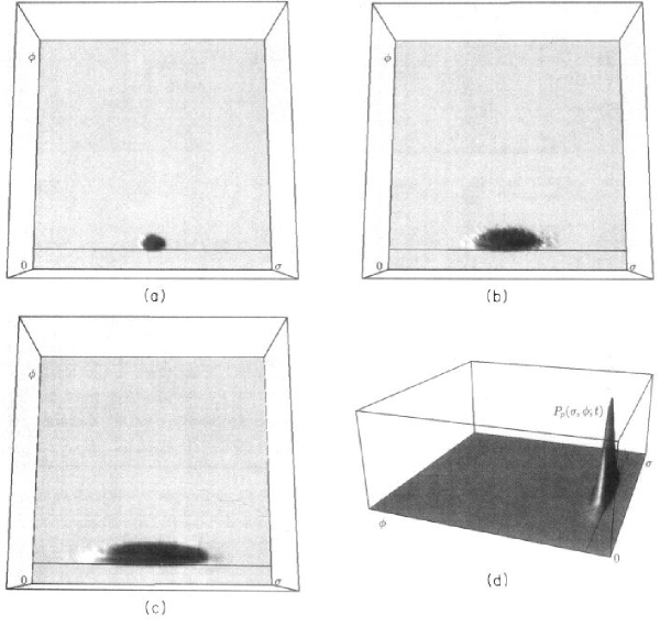
Figure 1: Diffusion of the distribution $P_{p}$ along the Planck boundary in the simplest theory with $V(\sigma)=const$, in the time $t$ parametrization. Figs. 1a, 1b, 1c show different steps towards stationarity at the Planck boundary. Fig. 1d shows the same stage of the diffusion as Fig. 1c, but in a different perspective.

To illustrate this feature, we performed computer simulation of diffusion for the simplest case of the theory with $V(\sigma)=const$, see Fig. 1. The first few images (Figs. 1a - 1c) correspond to the view “from the top”. The horizontal line across the box in Figs. 1a - 1c corresponds to the Planck boundary; the distribution $P_{p}$ is concentrated above this line. In the beginning we have a delta-functional distribution concentrated near some initial values of $\sigma$ and $\phi$. Then it rapidly moves towards the Planck boundary; it looks like a round spot from the viewpoint we have chosen, see Fig. 1a. After that the distribution widens in the $\sigma$-direction along the Planck boundary, while preserving its width in the $\phi$-direction orthogonal to this boundary, see Figs 1b, 1c. Its shape can be better understood from another viewpoint, see Fig. 1d, which shows the same distribution as Fig. 1c in a different perspective. The most important feature of this distribution is that its evolution very soon becomes effectively one-dimensional, being entirely concentrated near the Planck boundary. We will take advantage of this feature for the study of the runaway solutions in the next Section.

8 Runaway Solutions

Let us study the behavior of the probability distribution $P_{p}$ along the Planck boundary. In the case of an increasing potential like $\lambda\sigma^{2n}$, the larger the value of $\sigma$ in a given domain, the greater the increase in physical volume of that domain. Therefore, the probability distribution $P_{p}$ will tend to move towards large $\sigma$. The way it moves will depend on the type of potential. For some, as we will see, it is an explosive behavior. The probability distribution gives a statistical description of the quantum diffusion process towards large $\sigma$, but it proves useful to analyze the particular behavior of those relatively rare domains in which the field $\sigma$ increases in every quantum jump of amplitude $H/2\pi$. We can compute the speed at which those domains move towards large values of the field $\sigma$ from the equation (where $\Delta t=H^{-1}$)

$$\dot{\sigma}\equiv{\delta\sigma\over\Delta t}={H^{2}_{p}\over 2\pi}={4\over 3}\left({\lambda\over 2n}\right)^{1/2}\sigma^{n}\ ,$$ (49)

where $H_{p}$ is the Hubble parameter along the Planck boundary. For $n=1$ there is an exponential increase of $\sigma$ in those domains, while for $n>1$ we find an explosive solution

$$\sigma(t)=\sigma_{o}\ \left(1-{4(n-1)\over 3}\sqrt{\lambda\over 2n}\ \sigma_{o}^{n-1}\ t\right)^{-{1\over n-1}}\ .$$ (50)

We see that for all $n>1$ those first domains of the diffusion process reach infinity in finite time. Note that the total volume of such domains at that time will be finite, and then they will start growing at an infinitely large rate. This behavior is explosive and will correspond to probability distributions that are nonstationary and singular at $\sigma\to\infty$. It is extremely difficult to study this regime using computer simulations, but with the help of the results obtained in the previous section we can get a pretty good understanding of the behavior of $P_{p}$ in such a situation.

The qualitative analysis and the computer simulations of Section 5 suggest that the general solution to the diffusion equation for both fields will factorize naturally into a motion perpendicular to the Planck boundary that will reach stationarity very quickly, and a motion along it towards large values of $\sigma$. We will try to study this last motion in the absence of a boundary condition at $\sigma_{b}$. We assume that we can ignore the classical motion along the Planck boundary. Indeed, for large $\omega$ and small masses and coupling constants classical motion is almost exactly orthogonal to the Planck boundary. This assumption might be violated at large $\sigma$ for some theories with very rapidly growing potentials, but in the most interesting case of the theory $\lambda\sigma^{4}$ the classical motion is exactly orthogonal to the Planck boundary for all $\sigma$. On the other hand, for large $\omega$ and small masses and coupling constants the motion along the Planck boundary almost exactly coincides with the motion along the $\sigma$-axis. In this case an approximate diffusion equation for $P_{p}$ analogous to eq. (47) can then be written as follows:

$${\partial P_{p}\over\partial t}={1\over 8\pi^{2}}{\partial\over\partial\sigma}\left(H_{p}^{3/2}{\partial\over\partial\sigma}\left(H_{p}^{3/2}P_{p}\right)\right)+3H_{p}P_{p}\ ,$$ (51)

where the Hubble parameter along the Planck boundary in the theories with $V={\lambda\over 2n}\sigma^{2n}$ is given by

$$H_{p}^{2}={8\pi\over 3}{V(\sigma)\over M_{\rm p}^{2}(\phi)}={8\pi\over 3}V(\sigma)^{1/2}={8\pi\over 3}\left({\lambda\over 2n}\right)^{1/2}\sigma^{n}\ .$$ (52)

Equation (51) can be written as

$${\partial\Psi\over\partial u}={\partial^{2}\Psi\over\partial s^{2}}+a\ s^{p}\Psi\ ,$$ (53)

where

$$\begin{array}[]{c}{\displaystyle\Psi=\exp(Eu)H^{3/2}P_{p}\ ,\hskip 14.22636pt\hskip 14.22636ptu=\sqrt{8\over 27\pi}\left({\lambda\over 2n}\right)^{3/4}\left({4-3n\over 4}\right)^{2}t\ ,}\\[8.53581pt] {\displaystyle s=\sigma^{4-3n\over 4}\ ,\hskip 14.22636pt\hskip 14.22636pta=9\pi\left({4\over 4-3n}\right)^{2}\sqrt{2n\over\lambda}\ ,\hskip 14.22636pt\hskip 14.22636ptp={2n\over 4-3n}\ .}\end{array}$$ (54)

Let us first analyze the case $V(\sigma)=\lambda\sigma^{4}/4$. This corresponds to $p=-2$. It is clear from (53) that there are no stationary solutions to this equation in the absence of a boundary condition for $\sigma$. Furthermore, we know from quantum mechanics that potentials of the type $-1/s^{2}$ have singular solutions at $s=0$ ($\sigma=\infty$). Therefore we expect the distribution $P_{p}$ to be singular at $\sigma=\infty$. This was also expected from the analysis of those first domains that reach infinity in finite time.

On the other hand, for the theory $V(\sigma)=m^{2}\sigma^{2}/2$, the Schrödinger potential (53) is of the type $-s^{2}$, which has non singular solutions at large $\sigma$. For small $s$ the solution of eq. (53) is a Gaussian centered at $s(t)=\left\langle s\right\rangle$, with dispersion $\Delta(t)$. The potential then acts asymmetrically on it, pulling more at large $s$ and leaving a long exponential tail at small $s$. The maximum will move towards large $\sigma$, while maintaining a regular solution at infinity. This is expected from the previous analysis of the most rapid domains (49). For $n=1$ we find that the first domains will take an infinite time to reach infinity, giving a regular solution at any time.

However, in both cases we do not have runaway stationarity. Indeed, let us consider equation (51) and assume (for simplicity only) that in the very beginning the function $P_{p}$ was constant. Then both for $n=1$ and for $n=2$ the first term in the r.h.s. of this equation initially is positive. Neglecting this term, we obtain $P_{p}\sim\exp(3H(\sigma)t)$, which does not exhibit any runaway stationarity. Taking into account the first term in the r.h.s. of equation (51) makes the growth of $P_{p}$ at large $\sigma$ even faster. This confirms our expectations that in order to obtain runaway stationarity one should have an extremely flat effective potential.

9 Stationary Distributions for Various Theories

In this section we will study stationary probability distributions for several different potentials $V(\sigma)$. Our investigation will mainly rely on the results of our computer simulations, but we will try to make analytical investigation whenever possible. As we have argued in the previous sections, the simultaneous diffusion of both fields can be approximated by a quick diffusion in the $\phi$–direction towards the Planck boundary and a subsequent diffusion along it until it reaches the boundary at $\sigma=\sigma_{b}$, or until a stationary distribution is established for some other reason.

1) $V(\sigma)={\lambda\over 4}\,\sigma^{4}$. In this case the motion along the Planck boundary is governed by (53) with $p=-2$ and $a=72\pi/\sqrt{\lambda}$ and with the boundary conditions $\Psi(0)=\Psi(s_{b})=0$. It is difficult to find an exact analytical solution to this simple equation, but one can easily solve it in the WKB approximation,

$$\begin{array}[]{c}{\displaystyle\Psi(s)\sim\left(E-{a\over s^{2}}\right)^{-1/4}\exp\left[-(Es^{2}-a)^{1/2}+\sqrt{a}\ {\rm arcsec}\sqrt{Es^{2}\over a}\,\right],\hskip 14.22636ptEs^{2}>a,}\\[11.38109pt] {\displaystyle\Psi(s)\sim 2\left({a\over s^{2}}-E\right)^{-1/4}\cos\left[(a-Es^{2})^{1/2}-\sqrt{a}\ \ln\left({\sqrt{a}+(a-Es^{2})^{1/2}\over s\sqrt{E}}\right)+{\pi\over 4}\right],\hskip 14.22636ptEs^{2}<a,}\end{array}$$ (55)

where $E\simeq{72\pi\sigma_{b}\over\sqrt{\lambda}}\ (1-{3\over 4}(\pi\sqrt{\lambda}/6)^{1/3})$. This solution has a very sharp maximum close to the boundary $\sigma=\sigma_{b}$ and an exponential decay for small $\sigma$ (large $s^{2}=1/\sigma$). This behavior is precisely what we observe in the numerical solutions described below.

We take the following parameters for our computer simulations: $\omega=50$, $\lambda=0.3$. In the beginning of the series of calculations we took the points with coordinates $(\sigma,\phi)$ close to the Planck boundary, but in different initial positions with respect to the boundary $\sigma_{b}$. We have found that the duration of the intermediate non-stationary regime depends on the initial values of $\phi$ and $\sigma$. However, typically the stationary distribution $P_{p}(\sigma,\phi)$ is established very rapidly, after just a few steps $\Delta t\sim H^{-1}_{0}$. The resulting stationary distribution is presented in Fig. 2. Line OA at this figure corresponds to the end of inflation; there is no inflation for ($\sigma,\phi$) to the left of this line. Line OB corresponds to the Planck boundary; $V(\sigma)$ is greater than the Planck density $M_{\rm p}(\phi)$ under this line. The line $\sigma=\sigma_{b}$ is an additional boundary discussed above.

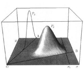
Figure 2: Stationary probability distribution $P_{p}$ in the plane $(\sigma,\phi)$ for the theory $V(\sigma)={\lambda\over 4}\sigma^{4}$, in the time $t$ parametrization. The line OA corresponds to the end of inflation, while the line OB to the Planck boundary. Inflation occurs between these two lines. The line above OA shows the probability distribution ${\cal P}_{p}$.

The curve above the line OA is of the most interest for us. It represents the stationary flow of domains crossing different parts of the boundary OA at the end of inflation. This gives us the probability distribution ${\cal P}_{p}(\phi_{e})$ that at the end of inflation the field $\phi$ takes some particular final value $\phi_{e}$. The maximum of this curve corresponds to the most probable value of the Planck mass $M_{\rm p}=\sqrt{2\pi\over\omega}\phi_{e}$ at the end of inflation. The top of the ‘mountain’, which shows the stationary distribution $P_{p}(\sigma,\phi)$, corresponds to the most probable value of $M_{\rm p}$ during inflation. Not unexpectedly, the curve above the line OA looks like a shadow of the mountain $P_{p}$. Indeed, as we have already mentioned, the distribution $P_{p}$ and the distribution ${\cal P}_{p}$ are directly related to each other, see (34). Meanwhile, the shape of the distribution $P_{p}$ at small $\sigma$ and large $\phi$ is obviously related to its shape at large $\sigma$ and small $\phi$, since in the intermediate regions the points ($\phi,\sigma$) follow classical circular trajectories, see e.g. (8). Consequently, the position of the maximum of ${\cal P}_{p}$ can be approximately obtained by drawing a circle with the center at $\phi=\sigma=0$, which goes through the crossing point of the Planck boundary and the boundary $\sigma=\sigma_{b}$.

2) $V(\sigma)={\lambda\sigma^{4}\over 4}\,\exp{\sigma^{4}\over\sigma_{0}^{4}}$. The exponential term is added here in order to show that one can avoid introducing additional boundaries at $\sigma=\sigma_{b}$ if the effective potential becomes very steep at large $\sigma$. The result is that the WKB solution (55), instead of decreasing sharply to $\sigma=\sigma_{b}$, decays exponentially fast. It is just the effect of substituting an infinite barrier by an exponential barrier. As we see in the numerical simulations, with a proper choice of the place where the effective potential becomes very steep one can reproduce the same result as if there were a boundary at $\sigma_{b}\sim\sigma_{0}$, see Fig. 3.

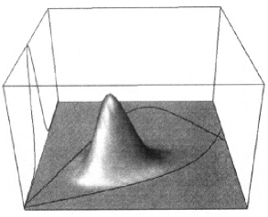
Figure 3: Same as in Fig. 2 for the potential $V(\sigma)={\lambda\sigma^{4}\over 4}\,\exp{\sigma^{4}\over\sigma_{0}^{4}}$. The distribution ${\cal P}_{p}$ is shown on the left side of the box.

In this figure we show the boundary of the end of inflation by a somewhat wavy line above the Planck boundary. At small $\sigma$ the boundary of the inflationary region goes as a straight line from the point $\sigma=0$, $\phi=0$ (compare to the line OA, Fig. 2), but then it becomes curved because of the exponential term which precludes inflation at large $\sigma$. Finally this line crosses the Planck boundary. The distribution $P_{p}$ is surrounded by this line and the Planck boundary.

On the left wall of the box we show the distribution ${\cal P}_{p}$, which in the previous picture we have shown above the line OA. In other figures we will do the same everywhere when the end of inflation boundary is significantly curved.

3) $V(\sigma)={\lambda\sigma^{4}\over 4}\,\exp(-{\sigma^{4}\over\sigma_{0}^{4}})$. In this case there is a sharp cut-off of the effective potential at $\sigma>\sigma_{0}$, which also leads to the existence of a stationary solution, as if there were a boundary near $\sigma_{0}$, see Fig. 4. As in Fig. 3, the wavy line corresponds to the end of inflation boundary.

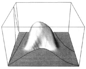
Figure 4: Same as in Fig. 1 for the potential $V(\sigma)={m^{2}\over 2}\sigma^{2}$.

4) $V(\sigma)={m^{2}\over 2}\sigma^{2}$. In this case the Planck boundary is not a straight line but a parabola $\phi^{2}={m\ \omega\over 2\pi\sqrt{2}}\ \sigma$. The eigenvalue equation associated with the probability distribution along the Planck boundary is (53) with $p=2$ and $a=144\pi\sqrt{2}/m$. In the WKB approximation

$$\begin{array}[]{c}{\displaystyle\Psi(s)\sim\left(E-as^{2}\right)^{-1/4}\exp\left[{s\over 2}(E-as^{2})^{1/2}+{E\over 2\sqrt{a}}\arcsin\sqrt{as^{2}\over E}-{\pi E\over 4\sqrt{a}}\right],\hskip 14.22636ptas^{2}<E\ ,}\\[8.53581pt] {\displaystyle\Psi(s)\sim 2\left(as^{2}-E\right)^{-1/4}\cos\left[{s\over 2}(as^{2}-E)^{1/2}-{E\over 2\sqrt{a}}\ln\left({s\sqrt{a}+(as^{2}-E)^{1/2}\over\sqrt{E}}\right)-{\pi\over 4}\right],\hskip 8.53581ptas^{2}>E\ ,}\end{array}$$ (56)

where $E\simeq{144\pi\sqrt{2\sigma_{b}}\over m}\ (1-({9\pi m\over 16\sqrt{2}\sigma_{b}})^{1/3})$. This solution has a very sharp maximum close to the boundary $\sigma=\sigma_{b}$ and an exponential decay for small $\sigma$ (small $s^{4}=\sigma$). This behavior is precisely what we observe in the numerical solutions. The distribution $P_{p}$ is very similar to that of the theory ${\lambda\over 4}\ \sigma^{4}$, see Fig. 5.

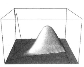
Figure 5: Same as in Fig. 3 for the potential $V(\sigma)={\lambda\sigma^{4}\over 4}\,\exp\Bigl{(}-{\sigma^{4}\over\sigma_{0}^{4}}\Bigr{)}$.

5) $V(\sigma)={m^{2}\over 2}\,\sigma^{2}+{\lambda\over 4}\sigma^{4}\log{\sigma\over\sigma_{0}}$. Naively, one could expect that the main part of the volume of the Universe in this model should originate as a result of inflation beginning from the points on the Planck boundary with the smallest angle $\theta$. Indeed, eq. (8) shows that the smaller is the initial angle, the greater is the degree of inflation [17]. However, due to the self-reproduction of inflationary domains and the more rapid expansion of domains with greater $\phi$ along the Planck boundary, the distribution $P_{p}$ does not stay near the point with the smallest $\theta$, but moves towards the largest possible $\phi$ and $\sigma$, see Fig. 6. As we discussed in the last section, this is a general result for any increasing potential, so $P_{p}$ is expected to have a maximum close to the boundary $\sigma=\sigma_{b}$.

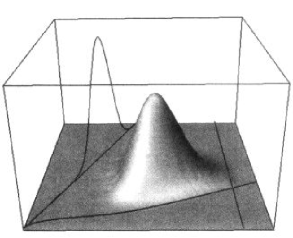
Figure 6: Same as in Fig. 1 for the potential $V(\sigma)={m^{2}\over 2}\,\sigma^{2}+{\lambda\over 4}\sigma^{4}\log{\sigma\over\sigma_{0}}$.

6) $V(\sigma)={1\over 4\lambda}(m^{2}-{\lambda\sigma^{2}})^{2}$. This is a typical potential used in the theories with spontaneous symmetry breaking. It has a minimum at $\sigma_{0}={m\over\sqrt{\lambda}}$. In this theory we have two alternative regimes. If one begins at $\sigma=0$, one may have an inflationary regime at small $\sigma$ [16], similar to the inflationary regime in the new inflationary universe scenario. If, on the other hand, inflation begins at large $\sigma$, then one has an inflationary regime similar to that in the theory ${m^{2}\over 2}\,\sigma^{2}+{\lambda\over 4}\sigma^{4}$. The only difference is that in the theory under consideration the field $\sigma$ eventually rolls down not to $\sigma=0$, but to $\sigma=\sigma_{0}$. The first possibility is illustrated by Fig. 7. On this figure the point $\sigma=0$ corresponds not to the left corner, as usual, but to the center of the $x$-axis.

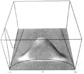
Figure 7: Same as in Fig. 1 for the potential $V(\sigma)={1\over 4\lambda}(m^{2}-{\lambda\sigma^{2}})^{2}$. It describes the stationary distribution for the case that inflation begins at $\sigma<\sigma_{o}$.

Note that if one begins with several inflationary domains with different initial conditions, at small $\sigma$ and at large $\sigma$, the domains with large $\sigma$ always win, and the distribution $P_{p}$ very soon becomes almost entirely concentrated at $\sigma>\sigma_{0}$, see Fig. 8.

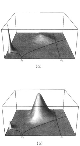
Figure 8: Same as in Fig. 7 for initial conditions both at large and small $\sigma$. This series of pictures shows that if one begins with equal number of “points” at large and at small $\sigma$, the volume corresponding to large $\sigma$ always dominates in the limit $t\to\infty$.

10 $\tau$–parametrization

The usual Fokker-Planck equation is written in terms of a time parameter $t$ as measured by the synchronized clocks of comoving observers. However, in general relativity one can use many different time parametrizations. For example, one can measure time by the local growth of the scale factor of the Universe and define a new time parameter [7]

$$\tau=\ln\frac{a(x,t)}{a(x,0)}=\int_{0}^{t}dt^{\prime}\ H(\sigma(x,t^{\prime}),\phi(x,t^{\prime}))\ .$$ (57)

This ‘time’ proves to be rather convenient since in this time, by definition, all parts of the Universe expand with the same speed $\sim e^{\tau}$, and $P_{p}$ is proportional (though not equal [10]) to $P_{c}$. One can easily derive the classical equations of motion and quantum diffusion in the new parametrization,

$$\frac{\partial\phi}{\partial\tau}=-\frac{M_{\rm p}^{2}(\phi)}{2\pi H}\ \frac{\partial H}{\partial\phi}\ ,\ \ \ \ \frac{\partial\sigma}{\partial\tau}=-\frac{M_{\rm p}^{2}(\phi)}{4\pi H}\ \frac{\partial H}{\partial\sigma}\ ,$$ (58)

$$\frac{\partial}{\partial\tau}\left\langle\phi^{2}\right\rangle=\frac{H^{2}}{4\pi^{2}}+{2\over\omega}\left\langle\phi^{2}\right\rangle\ ,\ \ \ \ \frac{\partial}{\partial\tau}\left\langle\sigma^{2}\right\rangle=\frac{H^{2}}{4\pi^{2}}-{2m^{2}\over 3H^{2}}\left\langle\sigma^{2}\right\rangle\ .$$ (59)

The conditions for the self-reproduction of the inflationary universe are the same as in the time $t$ parametrization (29). Furthermore, we are interested in the diffusion equation for the scalar fields in the physical frame, where $P_{p}(\sigma,\phi;\tau)=P_{c}(\sigma,\phi;\tau)\cdot e^{3\tau}$ satisfies

$$\begin{array}[]{rl}{\displaystyle\frac{\partial P_{p}}{\partial\tau}=}&{\displaystyle\frac{\partial}{\partial\sigma}\left(\frac{M_{\rm p}^{2}(\phi)}{4\pi H}\frac{\partial H}{\partial\sigma}P_{p}+\frac{H}{4\pi}\frac{\partial}{\partial\sigma}\left(\frac{H}{2\pi}P_{p}\right)\right)}\\[8.53581pt] +&{\displaystyle\frac{\partial}{\partial\phi}\left(\frac{M_{\rm p}^{2}(\phi)}{2\pi H}\frac{\partial H}{\partial\phi}P_{p}+\frac{H}{4\pi}\frac{\partial}{\partial\phi}\left(\frac{H}{2\pi}P_{p}\right)\right)+3P_{p}\ .}\end{array}$$ (60)

In this case, thanks to the absence of the $3HP_{p}$ term, there is a candidate for an exact stationary solution of eq. (60) given by

$$P_{p}(\sigma,\phi;\tau)\propto e^{3\tau}\,H^{-1}(\sigma,\phi)\exp\left({3M_{\rm p}^{4}(\phi)\over 8V(\sigma)}\right)\ .$$ (61)

Note that this expression is proportional to the square of the Hartle–Hawking wave function of the Universe. Unfortunately, this ‘stationary solution’ does not actually exist in any realistic model of inflation for the reason explained in [10]: The maximum of this distribution coincides with the position of the minimum of $V(\sigma)$ where there is no inflation and our stochastic equations do not apply. To find a correct solution, we should impose boundary conditions [10],

$$\begin{array}[]{c}{\displaystyle\frac{\partial}{\partial\sigma}\left(H(\sigma,\phi)P_{p}(\sigma,\phi)\right)|_{\rm end}=0\ ,}\\[8.53581pt] {\displaystyle P_{p}(\sigma,\phi)|_{\rm Planck}=0\ ,}\\[8.53581pt] {\displaystyle P_{p}(\sigma,\phi)|_{\sigma_{\phantom{}{}_{b}}}=0\ ,}\end{array}$$ (62)

which considerably modifies the shape of the distribution $P_{p}$. Nevertheless, the naive ‘solution’ (61) tells us something important about the shape of the distribution $P_{p}$. We expect this distribution to be peaked at the end of inflation boundary, instead of being concentrated near the Planck boundary as in the time $t$–parametrization. The exponent $\exp\left({3M_{\rm p}^{4}(\phi)\over 8V(\sigma)}\right)$ remains constant all the way along the end of inflation boundary for the theory $\lambda\sigma^{4}$. Therefore in this theory one expects the distribution to move towards small $\phi$ and $\sigma$, where the prefactor $H^{-1}$ in (61) is maximal. In other theories this argument does not apply, and in general one may obtain a stationary distribution with parameters depending not only on the boundary of the end of inflation but also on the boundary at $\sigma_{b}$. All these features are observed in the numerical simulations.

11 Computer Simulations of diffusion in time $\tau$

Computer simulations in the time $\tau$ are similar to the ones in the time $t$, but there are several important differences.

First of all, there is no need to make any splits of the domains. The reason is that all domains in the time $\tau$ expand with the same speed, by definition of this time as a logarithm of expansion. Each step of our calculation now corresponds to a time change $\Delta\tau=u$, where $u$ is some small number, $u<1$.

As before, evolution of the fields in each domain consists of several independent parts. Each field evolves according to classical equations of motion, (58), and in addition to it each field makes quantum jumps by $\delta\sigma={H\sqrt{u}\over\sqrt{2}\pi}\,\sin r_{1}$,  $\delta\phi={H\sqrt{u}\over\sqrt{2}\pi}\,\sin r_{2}$. Here $r_{1}$ and $r_{2}$ are random numbers which are different for each point.

As in Section 5, in addition to the distribution $P_{p}(\phi,\sigma,\tau)$ we computed also the volume of all domains where inflation ended within each new time interval $\Delta\tau$. This gives the fraction of the volume of the Universe where inflation ends at a given time $\tau$ within a given interval of values of the field $\phi$. We call this distribution ${\cal P}_{p}(\phi_{e},\tau)$. In the theories with $V(\sigma)=\frac{\lambda}{2n}\sigma^{2n}$

$${\cal P}_{p}(\phi_{e},\tau)\sim\phi_{e}\cdot P_{p}(\phi_{e},\sigma_{e},\tau)\ .$$ (63)

It is very instructive to compare the results of computer simulations in time $t$ and in time $\tau$ for various effective potentials $V(\sigma)$. The general tendency we observe is that the distribution $P_{p}(\phi,\sigma,\tau)$ is more closely concentrated not near the Planck boundary or near the boundary at large $\sigma$ (as was the case for the distribution $P_{p}(\phi,\sigma,t)$), but near the boundary corresponding to the end of inflation. The reason for this difference is very simple. In the time $\tau$ there is no additional enhancement of the volume filled by the fields corresponding to large values of the Hubble constant. Now let us consider several particular examples.

1) $V(\sigma)=const$. This corresponds to the simple model we considered in Section 6. In the time $t$ the distribution rapidly moved towards the Planck boundary and then diffused along it, Fig. 1. Evolution of $P_{p}$ in the time $\tau$ is quite different, for the reason discussed above. The distribution moves away from the Planck boundary, see Fig. 9. This explains many features of the distribution $P_{p}$ in more complicated theories to be considered below.

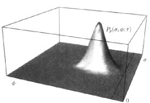
Figure 9: In the theory with $V(\sigma)=const$ the distribution $P_{p}(\phi,\sigma;\tau)$ moves away from the Planck boundary. Compare to Fig. 1d.

2) $V(\sigma)={\lambda\over 4}\,\sigma^{4}$. In this theory we do not have any typical mass scale which would correspond to a maximum of the probability distribution. Therefore in time $t$ the distribution was moving towards large $\sigma$ and $\phi$, until it was stabilized either by a boundary at large $\sigma$ or by the change of the potential at large $\sigma$ (e.g. $V(\sigma)={\lambda\over 4}\sigma^{4}\cdot\exp{\sigma^{4}\over\sigma_{0}^{4}}$, see next item). In the present case the distribution moves towards smaller and smaller $\sigma$ and $\phi$, and there is no stationary regime unless the potential $V(\sigma)$ at small $\sigma$ becomes, for example, quadratic in $\sigma$, see below. Fig. 10 shows how the distribution moves towards the corner $\sigma=\phi=0$. This Figure should be compared to Fig. 2, where the corresponding distribution is shown in time $t$.

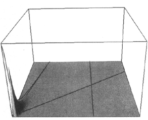
Figure 10: Probability distribution in the plane $(\sigma,\phi)$ for the theory $V(\sigma)={\lambda\over 4}\sigma^{4}$, in the time $\tau$ parametrization. Compare to Fig. 2.

As in the Section 5, the curve above the line corresponding to the end of inflation shows the probability distribution ${\cal P}_{p}(\phi_{e},\tau)$ that at the end of inflation the field $\phi$ takes some particular final value $\phi_{e}$. Note that in the present case this distribution depends on $\tau$ and moves towards $\phi_{e}=0$

3) $V(\sigma)={\lambda\over 4}\sigma^{4}\cdot\exp{\sigma^{4}\over\sigma_{0}^{4}}$. No qualitative difference appears here as compared with the theory ${\lambda\over 4}\,\sigma^{4}$ since the exponential term does not modify the potential at small $\sigma$.

4) $V(\sigma)={m^{2}\over 2}\sigma^{2}$. In this case the distribution $P_{p}$ is stationary, see Fig. 11. As one can see, it is concentrated near the boundary of the end of inflation. This Figure should be compared to Fig. 5.

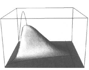
Figure 11: Same as in Fig. 10 for the theory $V(\sigma)={m^{2}\over 2}\sigma^{2}$.

5) $V(\sigma)={m^{2}\over 2}\,\sigma^{2}+{\lambda\over 4}\sigma^{4}\log{\sigma\over\sigma_{0}}$. In this model, and in a simpler model with $V(\sigma)={m^{2}\over 2}\,\sigma^{2}+{\lambda\over 4}\sigma^{4}$, the quadratic term stabilizes the distribution $P_{p}$, see Fig. 12. The resulting distribution is stationary even in the absence of the boundary at large $\sigma$; compare with Fig. 6.

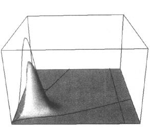
Figure 12: Same as in Fig. 10 for the potential $V(\sigma)={m^{2}\over 2}\,\sigma^{2}+{\lambda\over 4}\sigma^{4}\log{\sigma\over\sigma_{0}}$.

6) $V(\sigma)={1\over 4\lambda}(m^{2}-{\lambda\sigma^{2}})^{2}$. Here we have two alternative regimes. If one begins at large $\sigma$, then one has an inflationary regime similar to that in the theory ${m^{2}\over 2}\,\sigma^{2}+{\lambda\over 4}\sigma^{4}$. The corresponding distribution will be very similar to that shown in Fig. 12. One may have an inflationary regime at small $\sigma$ [16], similar to the inflationary regime in the new inflationary universe scenario. The corresponding distribution is shown in Fig. 13; compare with Fig. 7.

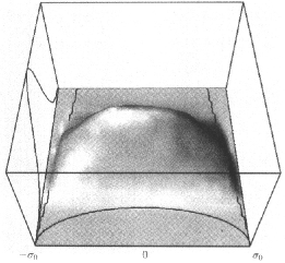
Figure 13: Same as in Fig. 10 for the potential $V(\sigma)={1\over 4\lambda}(m^{2}-{\lambda\sigma^{2}})^{2}$. It describes the stationary distribution for the case that inflation begins at $\sigma<\sigma_{o}$.

Note that the stationary distributions we have obtained look different from those for the same theories in time $t$. This means that the normalized distribution $P_{p}$ in the large time limit does not depend on time, but it does depend on the choice between different ‘times’ ($t,\tau$, etc.) A similar conclusion was earlier reached for other models studied in [10]. The reason of this strange behavior can be understood by using the following simple analogy.

Let us consider a two-dimensional plane $(x,y)$ and a cone formed by the lines $y=x$ and $y=-x$ going from the point $(0,0)$ towards positive $y$, see Fig. 14. Let us paint light grey the area inside this cone to the right of the $y$-axis, and paint gray the area inside the cone to the left of the $y$-axis. Now we will consider $y$ as a time direction, cross the cone by the lines of fixed $y$ at a distance $dy$ from each other and compare the white area and the gray area in the interval from $y$ to $y+dy$. Obviously, for all $dy$ the ratio of the white area to the gray area will be equal to 1, independently of the time $y$ (stationarity).

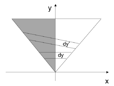
Figure 14: A cone in a two-dimensional space formed by the lines $y=x$ and $y=-x$. Two different parametrizations of “time” $y$ give different ratios for the gray over the white area, although they are both stationary.

Now one may choose another ‘time’ direction $y^{\prime}$ by rotating the $y$-axis, and slice the cone by the lines of constant $y^{\prime}$ and $y^{\prime}+dy^{\prime}$. In this case the ratio of the white area to the gray area in the interval from $y^{\prime}$ to $y^{\prime}+dy^{\prime}$ also will not depend on the time $y^{\prime}$ (stationarity), but this ratio will not be equal to 1 anymore. This strange effect is possible due to the fact that the total area of the gray part of the cone, as well as of the white one, is infinite. As usual, when the integrals are divergent, their ratio depends on the way one takes them. A similar effect appears in our case as well. The total volume of all inflationary domains in a self-reproducing universe is infinite in the limit $t\to\infty$ (or $\tau\to\infty$). Therefore the relative fraction of the volume of all domains with any particular properties may depend on the way in which we are sorting out these domains. This is the main reason of the difference between $P_{p}(\sigma,\phi;t)$ and $P_{p}(\sigma,\phi;\tau)$. This difference exists even if each distribution is stationary.

12 Discussion

Let us try to summarize our results and discuss their possible implications. First of all, we have confirmed that the regime of self-reproduction is possible not only in the ordinary inflationary theory, but in the Brans–Dicke inflation as well. However, the Brans–Dicke inflation has some new interesting features. In this theory the upper (Planck) boundary for the energy density of a classical space-time is not a point $V(\sigma)=M_{\rm p}^{4}$ as in the Einstein theory, but a line $V(\sigma)={4\pi^{2}\over\omega^{2}}\phi^{4}$. Similarly, the end of inflation boundary in the simplest models of chaotic inflation with $V(\sigma)\sim\sigma^{n}$ is not a point $\sigma\sim M_{\rm p}$ but a line $\sigma\sim\phi/\sqrt{\omega}$. In the ordinary inflationary models the probability distribution $P_{p}$ to find the inflaton field $\sigma$ at a given time in a given volume typically is concentrated either near the Planck boundary or near the boundary where inflation ends [10]. In the Brans–Dicke theory with $V(\sigma)\sim\sigma^{n}$ or with $V(\sigma)\sim e^{\alpha\sigma}$ this distribution also approaches one of these two boundaries, but after that it may continue moving, sliding along the boundaries.

As a result, the probability distribution $P_{p}$ approaches stationary regime only if there exist some additional reasons which preclude this sliding. This may happen, for example, if the effective potential becomes very steep (or if it decreases) at large $\sigma$. We have studied this possibility both by making computer simulations in the theories with potentials which become rapidly increasing (or decreasing) at large $\sigma$, and by introducing a phenomenological boundary at $\sigma=\sigma_{b}$. We obtained stationary probability distributions for a wide class of theories with two different time parametrizations.

If nothing precludes sliding of the probability distribution along the boundaries, one typically obtains a non-stationary distribution. However, the local stationarity still exists: The properties of domains with given values of scalar fields $\phi$ and $\sigma$ do not depend on the time when these domains were formed.

Whether the probability distribution $P_{p}$ is stationary or not, in the process of its evolution it probes all values of the fields $\phi$ and $\sigma$ for which inflation and self-reproduction of the Universe can take place. As a result, after inflation the Universe becomes divided into many exponentially large domains with different values of the effective Planck mass $M_{\rm p}(\phi)$.

It would be natural to assume that the probability to live in a typical part of our Universe is proportional (though not equal, see below) to ${\cal P}_{p}(\phi_{e})$. In particular, if our calculations would give us a delta-functional distribution ${\cal P}_{p}(\phi_{e})$, we would have a definite prediction for $M_{\rm p}$ and thus for $G$. Our results show, however, that the distributions which we obtain for large values of masses and coupling constants are rather smooth. If one takes very small masses and coupling constants, which is necessary to obtain small density perturbations $\delta\rho/\rho$, the distributions become very sharply peaked indeed, but still they are not delta-functional.

The probability to live in a given part of the Universe depends not only on its volume (which is proportional to the distributions $P_{p}$ and ${\cal P}_{p}$ if they are sufficiently narrow) but also on the conditions inside this volume. These conditions depend very strongly on the value of $M_{\rm p}$. For example, it is well known that a decrease of the Planck mass $M_{\rm p}$ by less than an order of magnitude from its present value in our part of the Universe would make the lifetime of the Sun so small that no biological molecules would appear on the Earth. An even bigger decrease of $M_{\rm p}$ would lead to an extremely efficient nucleosynthesis and to the absence of hydrogen in the Universe [26]. An increase of $M_{\rm p}$ would slow the expansion of the Universe. In such a Universe the departure from thermal equilibrium during the process of baryogenesis would be small, this process would be inefficient and the Universe now would be practically empty. On the other hand, a decrease of $M_{\rm p}$ decreases the reheating temperature after inflation, which may also cause the absence of baryons. Finally, in the simplest model of inflation with $V(\sigma)={m^{2}\over 2}\sigma^{2}$, density perturbations produced during inflation are inversely proportional to $M_{\rm p}$, see eq. (28). Therefore a change of $M_{\rm p}$ would lead to a profound modification of the properties of galaxies.

This suggests that the knowledge of the distribution ${\cal P}_{p}$ being complemented with anthropic considerations may help us determine the most probable value of the gravitational constant in the domains of the Universe where life of our type is possible. This is a very exciting possibility, resembling the ‘big fix’ paradigm of the baby universe theory [27], but, just like the baby universe theory, it involves many speculations. One of the problems of such an approach is the dependence of ${\cal P}_{p}$ on the choice of time parametrization. We will briefly discuss this issue in the Appendix. Whether this most ambitious part of our program will be successful or not, it is certainly true that the theory of a self-reproducing inflationary Brans–Dicke universe offers us many interesting and unexpected possibilities.

For example, in the standard inflationary cosmology the Planck mass was fixed, and in order to obtain a desirable amplitude of density perturbations ${\delta\rho\over\rho}\sim 5\cdot 10^{-5}$ in the theory ${m^{2}\over 2}\sigma^{2}$ one should introduce into the theory a new mass scale, $m\sim 10^{13}$ GeV, which is six orders of magnitude smaller that the Planck mass $M_{\rm p}\sim 10^{19}$ GeV. This cannot be considered as a fine tuning; after all, the electron mass is 22 orders of magnitude smaller than the Planck mass. Still it is very interesting to see how the same issue looks in the context of the inflationary Brans–Dicke theory.

In this theory $m$ is fixed but the Planck mass is not. It takes all its possible values in different parts of inflationary universe. Correspondingly, the amplitude of density perturbations in different parts of the Universe takes all possible values from $0$ to $O(1)$. If by calculating ${\cal P}_{p}$ and using anthropic considerations we are able to explain why we live in a part of the Universe with ${\delta\rho\over\rho}\sim 5\cdot 10^{-5}$ (see Appendix), then we will simultaneously explain why ${\delta\rho\over\rho}$ is so small and why $M_{\rm p}$ is so large in our part of the Universe. But there is a chance that we live in a part of the universe with ${\delta\rho\over\rho}\sim 5\cdot 10^{-5}$ without any special reason, just as some people live in exotic countries without even knowing that they are exotic. Nevertheless, even in this case we will get something interesting. We should simply look at equation (28) in a different way, writing it as follows:

$$M_{\rm p}(\phi)\sim 50\ m\cdot\left({\delta\rho\over\rho}\right)^{-1}\ .$$ (64)

This equation tells us that if we live in a part of the Universe with ${\delta\rho\over\rho}\sim 5\cdot 10^{-5}$, then in this part of the Universe the effective Planck mass automatically happens to be one million times larger than $m$, which is the only mass scale we have in our simple theory. In other words, we do not need to introduce into the theory two different mass scales different from each other by a factor of $10^{6}$. It is enough to have one mass scale; the rest of the job will be accomplished by quantum fluctuations in the inflationary universe. In this scenario both smallness of the density perturbations and greatness of the Planck mass appear as two sides of the same purely environmental effect.

The authors express their gratitude to A. Mezhlumian and V. Mukhanov for valuable discussions. The work of A.L. was supported in part by NSF grant PHY-8612280. The work of J.G.-B. was supported by a Spanish Government MEC-FPI postdoctoral grant.

Appendix.   Towards determination of the most probable value of the gravitational constant $G(\phi)$

One of the most interesting problems of elementary particle physics is to understand why the gravitational constant is so small or equivalently the Planck mass $M_{\rm p}$ is so large. In the context of our model this problem is formulated in a very unusual way. Our Universe consists of many exponentially large domains with different values of $G=M_{\rm p}^{-2}(\phi)$. Therefore instead of finding a unique value of $M_{\rm p}$ for the whole Universe, one should study the distribution of all possible values of $M_{\rm p}$ in our Universe. This might give us a possibility to understand why the gravitational constant is so small in the part of the Universe where we live.

First of all, one can make a natural assumption that the number of observers asking questions about the parts of the Universe with given values of fields $\phi$ and $\sigma$ is proportional to the volume of these parts. This suggests that the answer to our questions may be related to the investigation of the distributions $P_{p}$ and ${\cal P}_{p}$. However, it is not clear whether it is possible to justify this suggestion, especially if one recalls that these distributions depend on the choice of the time parametrization.

Note, that these probability distributions have a very well determined operational meaning when one uses them to predict the distribution of a scalar field in the Universe at a specific hypersurface $t=const$ (or $\tau=const$) under given initial conditions at $t=0$ (or at $\tau=0$). Now the main question is whether it is possible to use the results of our calculation of $P_{p}$ and ${\cal P}_{p}$ to get some information about the most probable value of the gravitational constant in those parts of the Universe where we can make observations and ask questions about the gravitational constant.

One may argue that as far as we have a nonvanishing probability to live in the domains with a given value of $M_{\rm p}(\phi)$, and as far as the total volume of all such domains integrated over all times is infinite (the integral exponentially diverges at $t\to\infty$), there is no reason to compare these infinities and study details of behavior of $P_{p}$. We live, which means that we have picked up one of these domains, but all attempts to go any further than that and to explain ‘our choice’ would not make any sense. This would be similar to attempts of a man from Switzerland to understand why he was born there rather than in China where the total number of people is much greater.

According to this point of view, one should use our results in a very limited way. One should find those domains where the distribution ${\cal P}_{p}$ and the probability of existence of life of our type do not vanish. (The answer to this question does not depend on the choice of time parametrization.) One should then find out what is the value of the effective Planck mass in each of these domains, and to relate it to other properties of space and matter in these domains.

In the Discussion we took this most conservative attitude towards our results. Even in this case inflationary cosmology goes far beyond the standard Big Bang paradigm, which assumes that the gravitational constant should be the same in all parts of our Universe.

This conservative attitude is quite legitimate. It is quite possible indeed that one should not ask why he or she was born in this or that country and in this or that part of the Universe. However, this idea is suspiciously similar to the old belief that it does not make any sense to question initial conditions in the Universe: The Universe is big and flat for the reason that it was born big and flat; it contains more baryons than antibaryons for the reason that it was created that way…  After the invention of the theory of baryogenesis and of inflationary cosmology this way of avoiding complicated problems does not look particularly attractive.

On the other hand, we are not well prepared to go beyond this point. In order to understand why do we live in a part of the Universe with a given value of the gravitational constant, one should learn first what is life, how it appears, is it correct that the probability for life to appear is proportional to the space available, etc. Before we do it, there will be no guarantee that we are on the right track. However, instead of waiting until the theory of everything is constructed, we may use inflationary cosmology as a good playground where we can test various hypotheses. This might help us to learn how to formulate correct questions (and, if we are lucky, to get correct answers) in the context of the new cosmological paradigm.

To illustrate some ambiguities involved in this approach, let us consider a problem formulated some time ago by Holger Nielsen [29]. Assume that we live in a peak of probability to be born at some particular time $t$. This hypothesis at the first glance looks quite reasonable and innocuous. In any case, it does not look obviously wrong if we are looking to the past. Indeed, the total population of the Earth now is much larger than it was before, and it continues growing exponentially. Most of the people who have ever lived on the Earth were born in the 20th century. This gives us a total of less than 20 billion people. If we assume that a typical person should be born near the maximum of the probability distribution, and if we assume that we are typical, then we would not expect much more that 20 billion people to be born from now on. But this is possible only if very soon, within the next few decades, the population of Earth will start rapidly decreasing [29].

We definitely want this doomsday prediction to be wrong, but what could be wrong about it? The point is that this prediction is a consequence of the assumption that the total number of people to be born is finite, and we live near the maximum of the distribution. However, if the total number of the people to be born is infinite, then we live at some time $t$ not for the reason that this time is near the maximum of the distribution, but for the only reason that we must pick up some finite time $t$ rather than the time $t=\infty$. For example, in our scenario the total volume of the Universe grows exponentially at all times. Consequently, the total number of domains of our type, the total number of planets of the type of the Earth and the total number of people populating these planets also grow exponentially [10]. Thus, in this scenario the total population of the Universe does not have any maximum and any falloff at large $t$.

This example shows that one should be extremely careful with probabilistic arguments to avoid many hidden ambiguities. For this reason we removed this discussion from the main body of the paper, to make sure that our speculations do not mix up with reliable results.

One of the obvious problems with the distributions $P_{p}$ and ${\cal P}_{p}$ is the choice of the time parametrization. Indeed, as we have seen, position of the peaks of these distributions does depend on this choice. Of course, one may argue that life as we know it uses ordinary time $t$ related to periodic processes, rather than the time $\tau$ which measures the logarithm of the distance between galaxies. Does it suggest that the proper distribution to study is $P_{p}(\sigma,\phi;t)$? Let us make this assumption for a moment and see what we will learn.

First of all, the peaks of the distributions $P_{p}$ for all theories we studied correspond to the state with a maximal possible value of the Hubble constant compatible with the self-reproduction of inflationary domains. For all theories $V(\sigma)\sim\sigma^{n}$ the peak of $P_{p}$ appears near the upper boundary $\sigma_{b}$, and the peak of ${\cal P}_{p}$ appears near $\phi\sim\sigma_{b}\sqrt{2\over n}$, which gives $M_{\rm p}\sim 2\sigma_{b}\sqrt{\pi\over\omega}$. The boundary $\sigma_{b}$ may correspond either to the place where $V(\sigma)$ changes its shape and becomes very steep, or to the place where it becomes decreasing.

Now one should multiply the volume of the domains with given $M_{\rm p}$ by the probability that life of our type can exist in these domains. The results look rather strange. Anthropic arguments seem to allow variations of $M_{\rm p}$ at least by one order of magnitude. Meanwhile typical distributions ${\cal P}_{p}$ are extremely sharp if masses and coupling constants are realistically small. Multiplication of these distributions typically gives a distribution which is sharply concentrated near one of the boundaries of the anthropically allowed region. This is very similar to the results obtained by Rubakov and Shaposhnikov when they discussed anthropic considerations in the context of the baby universe theory [30].

The situation becomes even more complicated when one considers models where the distributions $P_{p}$ and ${\cal P}_{p}$ are non-stationary. In such models the probability distribution ${\cal P}_{p}$ permanently moves towards infinitely large $\phi$. This growth eventually outweighs all anthropic bounds and pushes the distribution towards the region where life of our type could exist only as an extremely unstable phenomenon. This would be clearly incompatible with the results of anthropic considerations, which suggest that we live not far away from the center of the anthropically allowed region of possible values of $M_{\rm p}$.

One may try to interpret this conclusion as an argument against Brans–Dicke cosmology, or at least against those versions which lead to the runaway solutions for $P_{p}$ and ${\cal P}_{p}$. Another possibility is to use the distribution in the time $\tau$, which is typically much less sharp. Note that this time parametrization also has certain advantages, see [32]. Still another possibility is that the distributions $P_{p}$ and ${\cal P}_{p}$, being very useful for the description of the global structure of inflationary universe at a given time, cannot be used for the calculation of the probability of life appearing in the part of the Universe of our type. Indeed, as we know from [28], the notion of time (either $t$ or $\tau$) makes sense in the context of quantum cosmology only after the appearance of observers.

It is excitingly interesting to participate in the investigation of this problem. However, at the moment we do not even know whether physics provides a wide enough framework to study appearance of life, or some additional ingredients are needed [1]. This is an extremely complicated and speculative issue. We hope to return to its discussion in a separate publication. In the meantime we decided to restrict ourselves to the conservative approach outlined in the Discussion.

References

- [1] A.D. Linde, Particle Physics and Inflationary Cosmology (Harwood, Chur, Switzerland, 1990).
-
[2]
A.H. Guth, Phys. Rev. D 23, 347 (1981);
J.R. Gott, Nature 295, 304 (1982);
K. Sato, H. Kodama, M. Sasaki and K. Maeda, Phys. Lett. B 108, 35 (1982). - [3] P.J. Steinhardt, in The Very Early Universe, G.W. Gibbons, S.W. Hawking, S. Siklos, eds., Cambridge U.P. Cambridge, England (1982), p. 251; A.D. Linde, Nonsingular Regenerating Inflationary Universe, Cambridge University preprint (1982).
- [4] A. Vilenkin, Phys. Rev. D 27, 2848 (1983).
- [5] A.D. Linde, Phys. Lett. B 175, 395 (1986); Physica Scripta T15, 169 (1987); Physics Today 40, 61 (1987).
- [6] A.D. Linde, Phys. Lett. B 249, 18 (1990).
- [7] A.A. Starobinsky, in: Fundamental Interactions (MGPI Press, Moscow, 1984), p. 55; A.A. Starobinsky, in: Current Topics in Field Theory, Quantum Gravity and Strings, Lecture Notes in Physics, eds. H.J. de Vega and N. Sanchez (Springer, Heidelberg 1986) 206, p. 107.
- [8] A.S. Goncharov and A.D. Linde, Sov. Phys. JETP 65, 635 (1987); A.S. Goncharov, A.D. Linde and V.F. Mukhanov, Int. J. Mod. Phys. A2, 561 (1987).
- [9] Y. Nambu and M. Sasaki, Phys. Lett. B 219, 240 (1989); Y. Nambu, Prog. Theor. Phys. 81, 1037 (1989); M. Sasaki, Y. Nambu and K. Nakao, Phys. Lett. B 209, 197 (1988); Nucl. Phys. B 308, 868 (1988); K. Nakao, Y. Nambu and M. Sasaki, Prog. Theor. Phys. 80, 1041 (1988); M. Mijić, Phys. Rev. D 42, 2469 (1990); Int. J. Mod. Phys. A6, 2685 (1991).
- [10] A.D. Linde and A. Mezhlumian, Phys. Lett. B 307, 25 (1993); A.D. Linde, D.A. Linde and A. Mezhlumian, From the Big Bang Theory to the Theory of a Stationary Universe, Stanford University preprint SU-ITP-93-13, gr-qc/9306035 (Phys. Rev. D, to appear).
- [11] L.A. Kofman and A.D. Linde, Nucl. Phys. B282, 555 (1987).
- [12] S. Mollerach, S. Matarrese, A. Ortolan and F. Lucchin, Phys.Rev. D 44, 1670 (1991).
- [13] D. La and P.J. Steinhardt, Phys. Rev. Lett. 62, 376 (1989).
- [14] J.D. Barrow and K. Maeda, Nucl. Phys. B 341, 294 (1990); P.J. Steinhardt and F.S. Accetta, Phys. Rev. Lett. 64, 2740 (1990); J. García–Bellido and M. Quirós, Phys. Lett. B 243, 45 (1990); R. Crittenden and P.J. Steinhardt, Phys. Lett. B 293, 32 (1992); A.R. Liddle and D.H. Lyth, Phys. Lett. B 291, 391 (1992).
- [15] A.M. Laycock and A.R. Liddle, Sussex University preprint AST 93/6-1 (1993).
- [16] A.D. Linde, Hybrid Inflation, Stanford University Preprint SU-ITP-93-17, astro-ph/9307002 (Phys. Rev. D, to appear).
- [17] A.D. Linde, Phys. Lett. B 238, 160 (1990).
- [18] R.D. Reasenberg et. al., Astrophys. J. Lett. 234, L219 (1979); C.M. Will, Theory and experiment in gravitational physics (Cambridge U.P., 2nd ed., 1993)
- [19] J.A. Casas, J. García–Bellido and M. Quirós, Phys. Lett. B 278, 94 (1992); F.S. Accetta, L.M. Krauss and P. Romanelli, Phys. Lett. B 248, 146 (1990).
- [20] N. Deruelle, C. Gundlach and D. Langlois, Phys. Rev. D 46, 5337 (1992).
- [21] N.D. Birrel and P.C.W. Davies, Quantum Fields in Curved Space (Cambridge U.P., Cambridge, 1982).
- [22] A.L. Berkin and K. Maeda, Phys. Rev. D 44, 1691 (1991); S. Mollerach and S. Matarrese, Phys. Rev. D 45, 1961 (1991).
- [23] D.H. Lyth, Phys. Rev. D 31, 1792 (1985).
- [24] J. García–Bellido, Jordan–Brans–Dicke Stochastic Inflation, Stanford University preprint SU-ITP-93-36, astro-ph/9401042.
- [25] A.D. Linde, in The Very Early Universe, G.W. Gibbons, S.W. Hawking, S. Siklos, eds., Cambridge U.P. Cambridge, England (1982), p. 205; A. Borde, Class. Quant. Grav. 4, 343 (1987); A. Vilenkin, Phys. Rev. D 46, 2355 (1992); A. Borde and A. Vilenkin, Tufts University preprints, gr-qc/9312022 and gr-qc@xxx.lanl.gov - 9403004 (1994).
- [26] J.D. Barrow and F.J. Tipler, The Anthropic Cosmological Principle, (Oxford U.P., Oxford, 1986); I. L. Rosental, Big Bang, Big Bounce: How Particles and Fields Drive Cosmic Evolution (Springer, Berlin, 1988).
- [27] S. Coleman, Nucl. Phys. B 307, 867 (1988); Nucl. Phys. B 310, 643 (1989).
- [28] J.A. Wheeler, in: Relativity, Groups and Topology eds. C.M. DeWitt and J.A. Wheeler (Benjamin, New York, 1968); B.S. DeWitt, Phys. Rev. 160, 1113 (1967).
- [29] H.B. Nielsen, Acta Physica Polonica B20, 427 (1989).
- [30] V. Rubakov and M. Shaposhnikov, Mod. Phys. Lett. A4, 107 (1989).
- [31] L.J. Garay and J. García–Bellido, Nucl. Phys. B 400, 416 (1993).
- [32] D.S. Salopek and J.R. Bond, Phys. Rev. D42, 3936 (1990); ibid D43, 1005 (1991).