Impact of tangled magnetic fields on AGN-blown bubbles

Abstract

There is growing consensus that feedback from active galactic nuclei (AGN) is the main mechanism responsible for stopping cooling flows in clusters of galaxies. AGN are known to inflate buoyant bubbles that supply mechanical power to the intracluster gas (ICM). High Reynolds number hydrodynamical simulations show that such bubbles get entirely disrupted within 100 Myr, as they rise in cluster atmospheres, which is contrary to observations. This artificial mixing has consequences for models trying to quantify the amount of heating and star formation in cool core clusters of galaxies. It has been suggested that magnetic fields can stabilize bubbles against disruption. We perform magnetohydrodynamical (MHD) simulations of fossil bubbles in the presence of tangled magnetic fields using the high order PENCIL code. We focus on the physically-motivated case where thermal pressure dominates over magnetic pressure and consider randomly oriented fields with and without maximum helicity and a case where large scale external fields drape the bubble. We find that helicity has some stabilizing effect. However, unless the coherence length of magnetic fields exceeds the bubble size, the bubbles are quickly shredded. As observations of Hydra A suggest that lengthscale of magnetic fields may be smaller then typical bubble size, this may suggest that other mechanisms, such as viscosity, may be responsible for stabilizing the bubbles. However, since Faraday rotation observations of radio lobes do not constrain large scale ICM fields well if they are aligned with the bubble surface, the draping case may be a viable alternative solution to the problem. A generic feature found in our simulations is the formation of magnetic wakes where fields are ordered and amplified. We suggest that this effect could prevent evaporation by thermal conduction of cold H$\alpha$ filaments observed in the Perseus cluster.

1 Introduction

Active galactic nuclei play a central role in explaining the riddle of cool core clusters of galaxies. One of the unsolved problems of AGN feedback in clusters is the issue of morphology and stability of buoyant bubbles inflated by AGN and the efficiency of their mixing with the surrounding ICM. It is important to understand the process of bubble fragmentation and its eventual mixing with the rest of the ICM in order to quantify mass deposition and star formation rates in cool cores clusters. In the best-studied case of the Perseus cluster (Fabian et al. 2006) observations indicate that such bubbles can remain stable even far from cluster centers where they were created (see cup-shaped feature northwest of the center of the cluster or a similar yet tentative feature to the south in their Figure 3). One possible explanation for this phenomenon is that the intracluster medium is viscous and that viscosity suppresses Rayleigh-Taylor and Kelvin-Helmholz instabilities on their surfaces. Reynolds et al. (2005) performed a series of numerical experiments, compared inviscid and viscous cases and quantified how much viscosity is needed to prevent bubble disruption. For viscosity at the level of 25% of the Braginskii value they obtained results consistent with observations. The same problem has been considered analytically by Kaiser et al. (2005) who computed the instability growth rate as a function of scale and viscosity coefficient. An alternative possibility is that bubbles are made more stable by significant deceleration during their initial evolution (Pizzolato & Soker 2006). The “viscous solution” is very appealing as it also addresses the issue of dissipation of sound waves, weak shocks as well as $g-$modes (Fabian et al. 2003a). However, it is not entirely clear what the level and nature of viscosity in the ICM really is. This is because the ICM and the bubbles themselves are known to be magnetized and magnetic fields may reduce transport processes (but see Lazarian 2006 and Schekochihin & Cowley 2006). Although magnetic fields in clusters are known to have plasma $\beta>1$, ($\beta\equiv P_{\rm gas}/(B^{2}/2\mu_{o}$); e.g., Blanton et al. 2003) they may in principle have a strong effect on suppressing Kelvin-Helmholz and Rayleigh-Taylor instabilities. Jones & De Young (2005) considered the evolution of bubbles in a magnetized ICM by performing two-dimensional numerical MHD simulations and found that bubbles could be prevented from shredding even when $\beta$ is as high as $\sim 120$. A somewhat different conclusion was reached by Robinson et al. (2004) who simulated magnetized bubbles with the FLASH code (Fryxell et al. 2000) in two dimensions and found out that a dynamically important magnetic field ($\beta<1$) is required to maintain bubble integrity. Both of the above-mentioned simulations were performed in 2D and for very idealized magnetic field configurations such as, for example, doughnut-shaped fields with symmetry axis parallel to the direction of motion. Recently, Nakamura, Li, & Li (2006) considered the stability of Poyinting-flux dominated jets in cluster environment. Here we focus on a later stage in the outflow evolution and consider physically-motivated magnetic field case of $\beta>1$ and more realistic (stochastically tangled) field configurations in fossil bubbles (i.e., after the transition from the momentum-driven to buoyancy-driven stage) than in previous buoyant stage MHD simulations. We show that only when the power spectrum cutoff of magnetic field fluctuations is larger than the bubble size can the bubble shredding be suppressed. It is possible that such “draping” case is not representative of typical cool core fields (Vogt & Enßlin 2005) and, if so, other mechanism, such as viscosity, would be required to keep the bubbles stable. However, Vogt & Enßlin (2005) estimated magnetic power spectra in Hydra A only which shows extraordinarily strong AGN outbursts. We also note that such Faraday rotation observations of radio lobes are only weakly sensitive to large scale magnetic fields aligned with the bubble surface and rely on certain untested assumptions. Therefore, we argue that the draping case may be a viable solution to the problem of bubble stability.
In Section 2 we present the simulation setup and the justification for the parameter choices. Section 3 presents results and Section 4 our conclusions. The Appendix discusses in detail our method of setting up initial magnetic field configurations.

2 Simulation details

2.1 The code

The simulations were performed with the PENCIL code. (Dobler et al. 2003, Haugen et al. 2003, Brandenburg et al. 2004, Haugen et al. 2004) Although PENCIL is non-conservative, it is a highly accurate grid code that is sixth order in space and third order in time. It is particularly suited for weakly compressible turbulent MHD flows. Magnetic fields are implemented in terms of a vector potential so the field remains solenoidal throughout simulation (i.e., no divergence cleaning of the magnetic field is necessary). The code is memory efficient, uses Message-Passing Interface and is highly parallel. The PENCIL code is better suited for the simulations of stability of magnetized bubbles than smoothed particle magneto-hydrodynamical codes as it can better capture certain aspects of the bubble (magnetohydro) dynamics, such as Kelvin-Helmholtz instability, even for high density contrasts. and suffers less from numerical diffusion of the magnetic field. Although no formal code comparison has been made, other well known MHD mesh codes, such as FLASH or ZEUS, likely require comparatively higher resolution to achieve the same level of magnetic flux conservation as the PENCIL code.

2.2 Initial conditions

2.2.1 Density and temperature profiles

The cluster gas was assumed to be isothermal with temperature equal to 10 keV (this temperature was used to minimize the ratio of code viscosity to the Braginskii value; see Section 2.2.4 for more explanation). The gas was initially in hydrostatic equilibrium and subject to gravitational acceleration given by a sum of two isothermal potentials

$$g(r)=-\frac{2\sigma_{a}^{2}}{(r+r_{a})}-\frac{2\sigma_{b}^{2}}{(r+r_{b})},$$ (1)

where $\sigma_{a}=1.41$, $\sigma_{b}=2.69$, $r_{a}=30.0$ and $r_{b}=5.0$ in code units (see below) were the parameters were chosen to give a pressure profile consistent with that observed in clusters. Central gas density was $10^{-25}$ g cm^-3 (i.e., about $5.2\times 10^{-2}$ electrons per cm^-3). Self-gravity of the gas was neglected. The profiles of pressure and temperature are shown in Figure 1. We consider ideal gas with adiabatic equation of state with $\gamma=5/3$. The bubbles were underdense by a factor of ten with respect to the local ICM and its temperature was increased by the same factor to keep it in pressure equilibrium with the surrounding gas. The remaining bubble parameters are mentioned in section 2.2.4 where we discuss code units. The pressure in the ICM changes significantly over the height of the bubble. It is for this reason that we modified the density and temperature on a ”point-by-point” basis. That is, at every location within the bubble, we increased the temperature by a constant factor and decreased the density by the same factor while keeping the pressure at the same level as the pressure at the same distance from the cluster center away from the bubble. This way, the initial pressure distribution is smooth and there is no strong departure from perfect equilibrium. Although the density contrast of the bubble is relatively low, this has minimal effect on our results. This is because the buoyancy velocity is proportional to $(1-\rho_{\rm bubble}/\rho_{\rm icm})^{1/2}$ which is insensitive to $\rho_{\rm bubble}$ as long as it is much smaller than $\rho_{\rm icm}$. The reason we opted for such relatively low density contrast is numerical: higher bubble temperatures would have required smaller timesteps to achieve numerical stability. We also note that some real bubbles may have smaller density contrasts. A well-known extreme example is the Virgo cluster where buoyant bubbles in the radio show very little corresponding structure in the X-ray maps.

2.2.2 Magnetic fields

We consider magnetic fields inside the bubbles and in the ICM that are dynamically unimportant in the sense that their plasma $\beta$ parameter is greater than unity. That is, magnetic pressure may become important when compared to the bubble ram pressure associated with the gas motions in the ICM but it is generally small compared to the pressure of the ICM in our simulations. Analysis of cluster bubbles by Dunn et al. suggest that $\beta^{-1}$ is roughly in the range (10^-3, 0.3) with the mean $\langle\beta^{-1}\rangle=0.06$ and median of 0.03 (see sample of Dunn et al. 2004, Dunn et al. 2005 and Dunn 2006, Dunn priv. communication). Other evidence for high $\beta$ comes from observations of Faraday rotation measure and the lack of Faraday depolarization in bright X-ray shells in Abell 2052 as observed by Blanton et al. (2003). They infer $\beta\sim 30$. These arguments motivated us to consider high $\beta$ cases. However, we note that low-$\beta$ is not ruled out beyond reasonable doubt by the above observations and theoretical considerations and, thus, its consequences for bubble dynamics should be investigated further.
Regarding the geometry of magnetic fields, we consider random isotropic fields with coherence length smaller than the bubble sizes (hereafter termed “random”), isotropic helical fields with coherence length smaller then the bubble size (termed “helical” below; helicity is defined as $\int{\bf A}\cdot{\bf B}dV$, where ${\bf A}$ and ${\bf B}$ are vector potential and magnetic field respectively), and the “draping” case of isotropic fields characterized by coherence length exceeding bubble size as well as a non-magnetic case.
Magnetic draping has been considered previously in the context of merging cluster cores and radio bubbles using analytical approach by Lyutikov (2006). He found that even when magnetic fields are dynamically unimportant throughout the ICM, thin layer of dynamically important fields can form around merging dense substructure clumps (“bullets”) and prevent their disruption. We suggest that, depending on the unknown value of magnetic diffusivity, there may be some relic magnetic power spectrum with a smaller amplitude than the freshly injected one (either by AGN bubbles or dynamo-driven) that extends to scales larger than the bubble size and that provides draping fields to stabilize the bubbles.
The helical case is motivated by the fact that magnetic helicity is conserved for ideal MHD case. Moreover, helicity is proportional to the product of magnetic energy and typical lengthscale and, thus, fragmentation is not energetically preferred in the sense that it would lead to local increase of magnetic energy. Another justification for helical fields is that they may be responsible for explaining circular polarization of certain radio sources, and especially its sign persistency (Enßlin 2003 but see Ruszkowski & Begelman 2002). It is conceivable that magnetic helicity that could produce such signal in jets could survive till the buoyant stage.
The “random” case is motivated by the work of Vogt & Enßlin (2005) who estimate power spectrum of magnetic field fluctuations in Hydra A from Faraday rotation maps. We are conservative in our choice of parameters in the sense that we use fields of somewhat higher coherence length that are more likely to stabilize bubbles.

2.2.3 Vector potential setup

In setting up initial magnetic field configuration we ensured that the following conditions are met:

• magnetic fields must be divergence-free

• bubble and environmental fields must be isolated, i.e., no magnetic field lines should penetrate the surface of the bubble

• magnetic fields must be characterized by the required power spectra

• when necessary, magnetic helicity may be imposed

• magnetic plasma $\beta$ parameter of the bubble and the ICM must be independently controllable

• all considered field configurations must result (after suitable modifications) from the same white noise Gaussian random numbers. This ensures that the differences in evolution are entirely due to model parameters and not due to different random realizations.

The details of the algorithm used to set up the initial magnetic field configuration is presented in the Appendix..

2.2.4 Code units and resolution

We consider the the following code units: one length unit corresponds to 1 kpc, one velocity unit to 3$\times 10^{7}$ cm/s and one density unit to 10^-24 g/cm³. This corresponds to one time unit of approximately 3.3$\times 10^{6}$ years. The box size is 100 code length units on a side and shock-absorbing boundary conditions were used. This choice of boundary conditions was dictated by the fact that we wanted to exclude the Richmyer-Meshkov instability due to reflected waves passing through the bubble as a potential destabilizing mechanism. The bubble size was $d=25$ in diameter and its center was offset by 20 code length units from the cluster origin. The bubble was underdense by a factor of ten with respect to the local ICM and its temperature was increased by the same factor to keep it in pressure equilibrium with the surrounding gas. Our grid size is 200³ zones. The PENCIL code requires some viscosity and resistivity to run properly. Minimum required amount of physical viscosity that the code needs to prevent numerical instabilities from developing decreases as the numerical resolution is increased. We use viscosity $\nu=0.07$ and magnetic resistivity $\eta=0.07$. For typical values of electron density ($\sim 0.01$ cm^-3) and temperature (10 keV) in our simulations this value of viscosity corresponds to 0.014 of the Braginskii value. We note that for lower gas temperatures this ratio would be higher which motivated our choice of temperature. For the parameters considered here, in the initial stages in our simulations, maximum velocities in code units are roughly $u_{\rm max}\sim 6$. Note that for the adopted parameters the sound speed in the ICM is $c_{s}=5.44$ but the gas inside the bubbles is much hotter and so the actual gas velocities can be higher then $u_{\rm max}$ without “violating” the sound speed limit. For the bubble size $d=25$ and gas velocity $u_{\rm max}=6.0$, hydrodynamical and magnetic Reynolds numbers are roughly $Re=u_{\rm max}d/\nu\sim 2000$. Such values clearly lead to quick development of Rayleigh-Taylor and Kelvin-Helmholtz instabilities for unmagnetized bubbles.

3 Results

Figure 1: Initial pressure (solid line) and temperature profiles.

Figure 2: One dimensional energy power spectra of initial magnetic field fluctuations. Solid line shows energy spectrum corresponding to our “draping”. Dashed line is for the “random” case.

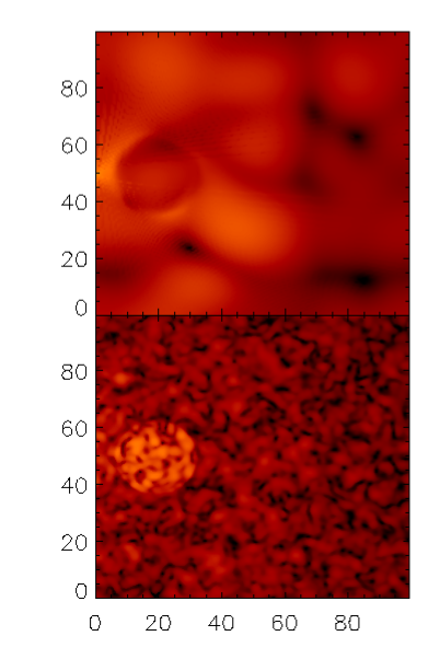
Figure 3: Magnetic pressure in the plane containing the cluster and bubble centers. Upper and lower panels show “draping” and “random” cases, respectively. The coherence length in the lower panel is even smaller than that used in the simulations to demonstrate the robustness of the method. See Appendix for more explanation.

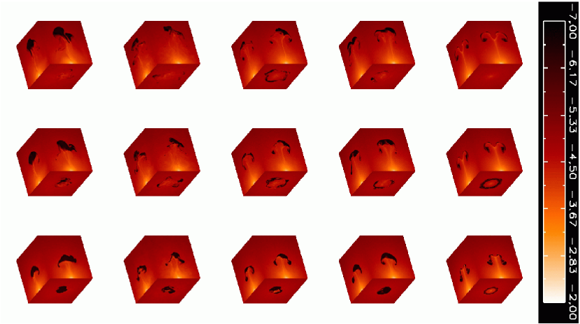
Figure 4: Natural logarithm of density in the cluster. Columns show time sequences of density for draping, random (i), random (ii), helical and non-magnetic cases from left column to the right, respectively. Rows correspond to time of 15.0, 25.0, 35.0 code time units from bottom to top. Sides of all boxes show densities in the planes intersecting the box and containing its center.

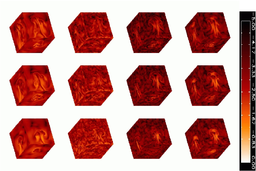
Figure 5: Magnetic pressure structure in the cluster. Columns show time sequences of magnetic pressure for draping, random (i), random (ii) and helical cases from left column to the right, respectively. Rows correspond to time of 0.0, 15.0, 25.0, 35.0 code time units from bottom to top.

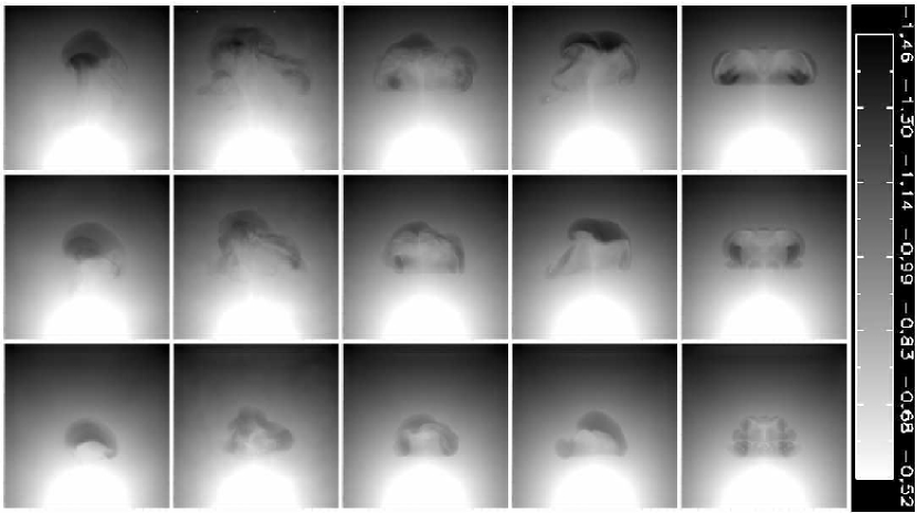
Figure 6: X-ray images of the cluster center. Columns show time sequences of X-ray emission for draping, random (i), random (ii) helical, and non-magnetic cases from left column to the right, respectively. Rows correspond to time of 15.0, 25.0, 35.0 code time units from bottom to top. Rows 1 to 3 correspond to a different projection axis than rows 4 to 6.

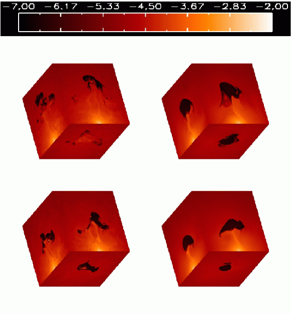
Figure 7: Natural logarithm of density distribution. Left column shows density for the random (i) case (lower panel t=15, upper t = 25 code time units) but twice as high mean magnetic pressure. Right column corresponds to the draping case for twice the mean magnetic pressure compared to the original draping case.

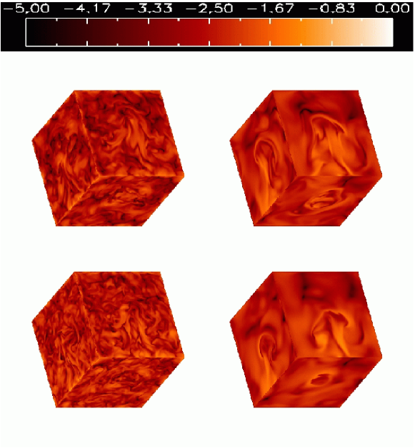
Figure 8: Same as Figure 7 but for the logarithm of magnetic pressure distribution. Note that in the draping case (right panel), a layer of ordered and amplified magnetic field forms on the bubble-ICM interface and protects the bubble against disruption.

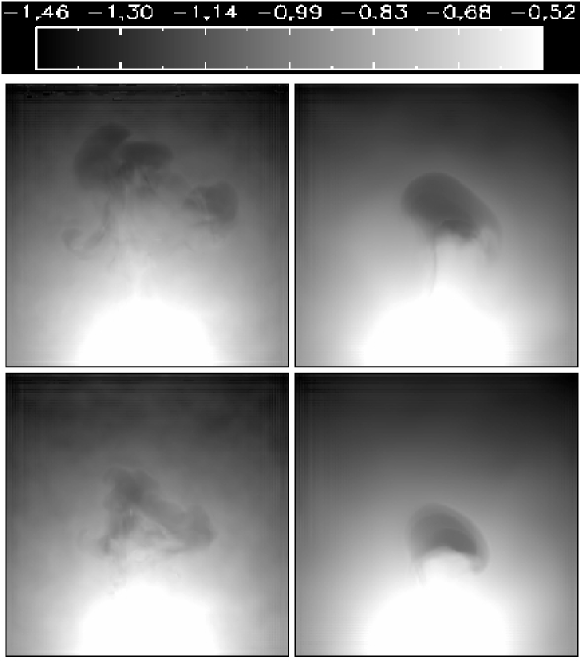
Figure 9: X-ray maps corresponding to Figures 8 and 9. Projection orientation is the same as in the upper panels in Figure 6.

Figure 10: Evolution of the mean magnetic pressure (averaged in the plane containing the cluster center and the initial bubble location) compared to gas pressure for the draping (solid lines) and random (i) cases. Lower panel is for twice the original mean initial magnetic pressure.

In Figure 4 we show the evolution of the gas density. Each column corresponds to one model. Time increases from bottom to top. Snapshots were taken at 15, 25, 35 code time units. The following five models were considered (from left to right):

• draping model: mean $\beta\sim 40$ throughout the box (i.e., relative plasma $\beta$ of the bubble with respect to the ICM is set to unity)

• random (i) model: constant mean $\beta$ throughout the box. The initial mean $\beta$ was chosen so as to match mean $\beta$ values near $t=15$ code time units in the draping case

• random (ii) model : initial bubble-averaged beta inside the bubble the same as the mean initial $\beta$ in case random (i) Relative magnetic pressure inside the bubble was chosen to be 10 times higher than the typical ambient magnetic pressure

• helical case: same as random (ii) but for helical fields

• non-magnetic case.

It is evident that the bubble morphology depends strongly on the topology of the initial magnetic field. There is a striking difference between draping case (first column) and all remaining cases. Even though magnetic fields are “dynamically” unimportant in the sense that the typical plasma $\beta$ parameter is much greater than unity, the bubble clearly is more coherent in the draping case than in any other case. The cup-shaped morphology in the draping case in the first snapshot at 15 time units is very reminiscent of the fossil bubble seen in the Perseus cluster. As the bubble moves up, its shape changes and it becomes more round. The Rayleigh-Taylor instability is prevented and so there is no evidence for strong contamination or mixing of the bubble interior with the colder ICM material. However, denser and colder material lifted by the rising bubble reverses its motion at a certain time and begins to fall back. This leads to some stretching of the bubble in the vertical direction in the later stages in its evolution.
The second column shows random (i) case. Here the gas behind the bubble quickly penetrates its center and tends to pierce through it. This is evident especially when the left hand sides of the cubes in the first and second column are compared. The working surface of the bubble becomes irregular and starts to fragment. Similar behavior is observed in the random (ii) case (third column). The two cases differ in the strength of magnetic field with case (ii) having stronger internal bubble fields but weaker ICM ones. Nevertheless, there does not seem to be much qualitative difference between these two cases in terms of density distribution.
The fourth column shows the helical case. The degree of bubble fragmentation is lower than in the random cases even though typical magnetic field strength is similar to that of random (i) case. Although this appears to be a weak effect, as explained in Section 2.2.2, helicity conservation should tend to stabilize the flow. This column should be compared mainly with the third column that shows its non-helical analog.
The last column shows the non-magnetic case. Both Rayleigh-Taylor and Kelvin-Helmholz instabilities develop here very quickly. The bubble is pierced by a column of cold gas forming a “smoke ring” rather then cup-shaped or oval structure as in the draping case. The edges of this ring are initially wrinkled by Kelvin-Helmholz instability.
In Figure 5 we show the distribution of magnetic pressure. As in Figure 4, columns correspond to different models and are ordered the same way while rows correspond to 15, 25, 35 time units from bottom to top. This figure reveals that the reason for bubble stability in the draping case (first column) is the formation of an “umbrella” or a thin protective magnetic layer on the bubble working surface that suppresses instabilities. Visual inspection of the figure comparing magnetic pressure evolution in the draping, two random, and helical cases shows that the field geometry does not change significantly (in the average sense) far away from the bubbles. The upward motion of the bubble also leads to substantial amplification and ordering of magnetic field in the bubble wake. This has consequences for estimates of conduction in the ICM based on the appearance of H$\alpha$ filaments (Fabian et al. 2003b, Hatch et al. 2006). It has been argued (e.g., Nipoti & Binney 2004) that thermal conduction has to be strongly suppressed in the ICM or otherwise such cold filaments would be rapidly evaporated. Our result hints at a possibility that thermal conduction may be locally weaker in the bubble wake, thus preventing or slowing down filament evaporation.
The second column shows random (i) case. No “umbrella” effect seen in the draping case is observed here. The fact that the colder gas enters the bubble from beneath does not lead to compression of magnetic field in the direction parallel to the bubble surface, an effect that could prevent disruption. Even though the bubble does get disrupted, some compression and ordering of magnetic field in the wake occurs here just as in the draping case. In fact, this effect is a generic feature of all the runs that we performed. The behavior of magnetic pressure in random (ii) case, shown in the third column, is qualitatively very similar with the difference that the magnetic wakes are more pronounced. Even though magnetic fields get marginally compressed near the bubble working surface in this case, they remain disjoint and do not prevent the shredding of the bubble.
The last column shows magnetic pressure in the helical case. There is a significant difference in the topology of the field inside the bubble between this and all previous cases. Here, the upward drift of the bubble appears to amplify magnetic field inside the bubble. Note that while in the draping case amplification took place in a thin layer coinciding with the working surface of the bubble, the amplification in the helical case is distributed throughout the bubble. This is particularly obvious in the snapshot taken at 15 code time units. We note that this means that moderate stabilizing effect of helicity comes from fields internal to the bubble rather than external ones as in the draping case. No obvious amplification inside the bubble is seen in the random cases other than the “wake” amplification.
In Figure 6 we show X-ray maps. The columns are arranged the same way as in Figure 4. Rows from 1 to 3 correspond to different projection direction than rows 4 to 6 (the latter ones correspond to the viewing direction rotated by 90 degrees around the axis intersecting the cluster center and the original location of the bubble). As expected, the morphology in the draping case is very different than in all other cases. In this case the bubbles show up as depressions in X-ray emissivity. The bubbles in the random case appear irregular. They are also brighter in their centers which is contrary to observations. In the helical case, the bubbles seem somewhat less disturbed than in the random case. It is possible that this case, when “observed” in synthetic Chandra data that includes instrument responses would resemble actual bubbles more than the random case bubbles. The last column shows the non-magnetic case that is clearly inconsistent with observations. Here the bubble more resembles two isolated bubbles than a coherent feature seen in the draping case. We suggest that a hybrid model that combines internal helical magnetic fields inside the bubble with external draping fields may produce X-ray bubbles that closely resemble bubbles seen in clusters. However, different method for setting up initial conditions than the one considered here would have to be employed to model such a case while ensuring that the initial magnetic field configuration does not suffer from any artifacts.
We note that the magnetic fields in our simulations are observed to decay with time. The decay is expected as, apart from the bubble-induced motion, the turbulence is not continuously driven in our simulations. As expected, the decay is faster for more tangled fields. Even though the field decays, we note that disruption (when present) is initiated early on in the bubble evolution. Moreover, our field strengths are greater than those in Jones & De Young (2005) uniform field case and yet we do observe disruption. We quantified the decay in magnetic pressure for the cases where the mean bubble and ICM $\beta$ parameters are the same (“draping” and random (i) cases). In Figure 10 we show the evolution of the mean magnetic pressure compared to gas pressure in the plane intersecting the cluster center and the original bubble location. We found that, while the ”random” case shows the decay, the ”draping” case is consistent with no decay. By construction, the mean fields in the draping case and random (i) one approximately match at $t=15$ code time units. The decay of the field after this time is rather slow and magnetic field strengths in the random and draping cases are comparable around and after this time. Prior to $t=15$ the field in the random case exceeds that in the draping case. It is interesting that, even though this is the case, the random case fields lead to bubble disruption while the draping case shows much more coherent structures. This demonstrates that the difference between this two cases is primarily due to the field geometry and not its strength, at least for the typical plasma $\beta$ considered here. Moreover, if we would have considered driven turbulence then we could have afforded to start from weaker fields in the random case and additional random motions due to turbulence driving would be present. Both of these effects (i.e., weaker initial field in conjunction with additional random motions) could only strengthen our conclusion, i.e., make the random case bubbles fragment even more easily. We are thus conservative in neglecting turbulence driving. We also note that our aim was not to address the stability of the bubbles exposed to random motions. Our objective was to discuss the effect of tangled magnetic fields on the development of Rayleigh-Taylor and Kelvin-Helmholz instabilities. Random motions, be it due to turbulence driving or due to post-merger relaxation, are inevitably going to be present in cool cluster cores (even though cool cores tend to be more relaxed than the centers of non-cooling flow clusters). Their impact has to be evaluated in evaluated in sepatate studies. Another unknown factor is how magnetic fields are driven inside the cavities (if at all). However, including such effects would be beyond the scope of our investigation.

3.1 Varying magnetic pressure

We simulated draping and random case (i) again for exactly the same parameters as before except for twice as high mean magnetic pressures in both cases. We observe the same trends with the difference that the draping case results in slightly more coherent bubbles while the random case in slightly more fragmented ones. This strengthens our arguments presented above that it is the geometry of the field rather than its strength that is responsible for stabilizing the bubbles (at least for the parameters considered here). In Figures 7, 8, and 9 we show density, magnetic pressure and X-ray emissivity, respectively. Note that the “umbrella” effect mentioned above is clearly seen in the draping case in the left column in Figure 8. This is to be contrasted with the left hand panel corresponding to the high magnetic version of the random (i) case where no such effect is observed. Lower panel in Figure 10 shows the evolution of the mean magnetic pressure compared to the gas pressure in the plane containing the center of the cluster and the initial position of the bubble.

4 Conclusions

We considered three-dimensional MHD simulations of buoyant bubbles in cluster atmospheres for varying magnetic field strengths characterized by plasma $\beta>1$ and for varying field topologies. We find that field topology plays a key role in controlling the mixing of bubbles with the surrounding ICM. We show that large scale external fields are more likely to stabilize bubbles than internal ones but a moderate stabilizing effect due to magnetic helicity can make internal fields play a role too. We demonstrate that bubble morphology closely resembling fossil bubbles in the Perseus cluster could be realized if the coherence of magnetic field is greater than the typical bubble size. While it is not clear if such a “draping” case is representative of typical cluster fields, Vogt & Enßlin (2005) find that length scale of magnetic fields in Hydra A is smaller than typical bubble size. If this also holds true in other clusters then other mechanisms, such as viscosity, would be required to keep the bubbles stable. Unfortunately, Faraday rotation method used by Vogt & Enßlin (2005) is not very sensitive to large scale magnetic fields if aligned with the bubble surface. Moreover, their maximum Likelihood method assumes a power-law relation between magnetic field and density, statistical isotropy for the purpose of deprojection and a particular jet angle with respect to the line-of-sight. Smaller angles and different magnetic field configurations might yield a weaker decline of the power spectrum at larger scales. Taking into account the above limitations, it is entirely possible that the draping case offers a viable alternative solution to the problem of bubble stability. We also suggest that a hybrid model that combines helical fields inside the bubble with external draping fields could be successful in explaining morphologies of X-ray bubbles in clusters. Another possibility is that dynamically significant fields are be present inside the bubbles and the consequences of high-$\beta$ case for bubble dynamics and stability should be investigated further. We note that the bubbles will most likely eventually get disrupted (partially helped by “cosmological” sloshing gas motions in clusters).
A generic feature found in our simulations is the formation of a magnetic wake where fields are ordered and amplified. We suggest that this effect could prevent evaporation by thermal conduction of cold H$\alpha$ filaments observed in the Perseus cluster.
The physical process of bubble mixing in the presence of magnetic fields has important consequences also for modeling of mass deposition and star formation rates in cool core clusters as well as the particle content of bubbles and cosmic ray diffusion from them. These issues will be further complicated by the effects of anisotropy of transport processes due to magnetic fields. This may give rise to the onset of magneto-thermal instability on the bubble-ICM interface (Balbus 2004, Parrish & Stone 2005). Studying such effects is beyond the scope of the present paper but certainly deserves further investigation.

5 Acknowledgements

We thank the referee for a detailed and insightful report. MR thanks Axel Brandenburg, Kandu Subramanian, Maxim Lyutikov, Eugene Churazov, Debora Sijacki, Jonathan Dursi, Maxim Markevitch, Alexei Vikhlinin and Alexander Schekochihin for helpful discussions. Test runs were performed on IBM p690 Regatta cluster at Rechenzentrum Garching at the Max-Planck-Institut für Plasmaphysik. Final production runs were performed on the Columbia supercomputer at NASA NAS Ames center. It is MR’s pleasure to thank the staff of NAS, and especially Johnny Chang and Art Lazanoff, for their their highly professional help. The Pencil Code community is thanked for making the code publicly available. The main code website is located at http://www.nordita.dk/software/pencil-code/. MB acknowledges support by the Deutsche Forschungsgemeinschaft.

6 Appendix

Initial magnetic fields were computed outside the main code and the setup was performed in two stages. In the first phase, we generated stochastic fields by three-dimensional inverse Fourier transform (FFT) of magnetic field that in ${\bf k}$-space had the amplitude given by

$$B\propto k^{-11/6}\exp(-(k/k_{1})^{4})\exp(-k_{2}/k),$$ (2)

where $k=(k_{x}^{2}+k_{y}^{2}+k_{z}^{2})^{1/2}$, and $k_{1}=2\pi/dx$, $k_{2}=0.3$, $dx=x_{\rm box}/32$, $x_{\rm box}=10^{2}$ for helical or random cases and $k_{1}=2\pi/(2r_{\rm bub})$ and $k_{2}=0.05$ in the draping case, where $x_{\rm box}$ is the size of the computational box in code units. (see below)
All three components of magnetic field were treated independently which ensured that the final distribution of ${\bf B}({\bf r})$ had random phase. That is, for example for the x component of the magnetic field, we set up a complex field such that

$$({\rm Re}({B_{x}}({\bf k})),{\rm Im}({B_{x}}({\bf k})))=(G(u_{1})B,G(u_{2})B),$$ (3)

where $G$ is a function of a uniform random deviate $u_{1}$ or $u_{2}$ that returns Gaussian-distributed values. For vanishing exponential cutoff terms, the above prescription would give classical Kolmogorov turbulence spectrum. Whereas there is no generally accepted justification for magnetic spectrum to have a Kolmogorov distribution, our parameter choice for the “random” case resembles that seen in the Hydra cluster (Vogt & Enßlin 2005). One-dimensional energy power spectra $kE(k)$ [erg s^-1 cm${}^{-3}]$ of magnetic field fluctuations are shown in Figure 2.
After the initial field has been set up in k-space, we implement a magnetically isolated bubble. This phase is performed according to the following iterative scheme:

(1) divergence cleaning in ${\bf k}$-space:

$${\bf B}({\bf k})\longmapsto({\bf 1}-\hat{\bf k}\hat{\bf k}){\bf B}({\bf k}),$$ (4)

where $\hat{\bf k}$ is a unit vector in ${\bf k}$-space. In the case of helical fields we also act on the field with helicity operator defined as:

$${\bf B}({\bf k})\longmapsto\frac{{\bf 1}+\alpha i\hat{\bf k}\times}{(1+\alpha^{2})^{1/2}}{\bf B}({\bf k}),$$ (5)

where $\alpha=1$ (maximum helicity case). The helicity step is only performed in the first loop of the iteration. Note that imposing helicity on the field does not change the power spectrum of magnetic energy fluctuations.

(2) inverse FFT of the new ${\bf B(k)}$ to real space. Each component of ${\bf B(k)}$ is independently acted upon with a three-dimensional inverse FFT.

(3) applying a projection operator to isolate the bubble magnetically. The projection operation modifies the field in the following way

$${\bf B}({\bf r})\longmapsto[{\bf 1}-g(r)\hat{\bf r}\hat{\bf r}]{\bf B}({\bf r}),$$ (6)

where $\hat{\bf r}$ is a unit vector in real space, $r$ is the distance from the bubble center, and $g(r)=1-|\cos[0.5\pi(x+\Delta x-1)/\Delta x]|$ for $1-\Delta x<x<1+\Delta x$ and $g(r)=0$ otherwise and $\Delta x=0.25$, where $x=r/r_{\rm bub}$. Note that both the field just inside and outside the bubble are acted upon by this operator. Applying this operator results in a field that possesses some divergence.

(4) changing relative magnetic pressure inside the bubble (done only during the first loop of the iteration process) Plasma $\beta$ parameter is given by $\beta(r)=\beta_{\rm rel}g_{b}(r)+1-g_{r}(r)$, where $\beta_{\rm rel}$ is the relative plasma $\beta$ parameter between the ICM and the bubble. The $g_{b}(r)$ term is given by $g_{b}(r)=1+\cos[0.5\pi(x+\Delta_{b}x-1)/\Delta_{b}x]$, where $x=r/r_{\rm bub}$ for $1<x<1+\Delta_{b}x$ and $g(r)=0$ otherwise. In the above expression, $r_{\rm bub}$ is the bubble radius and $\Delta_{b}x=0.15$.

(5) computing the FFT of ${\bf B}({\bf r})$ and going back to (1). Iterations are performed until the following convergence criterion is met: $\int(\nabla\cdot{\bf B}({\bf r}))^{2}dVdx^{2}/\int B^{2}dV<10^{-4}$, where integrations are performed for $|x-1|<\Delta x$.

At this point a convergent and divergence-free ${\bf B}({\bf r})$ field has been set up. Inverting such field to obtain the vector potential ${\bf A}({\bf r})$ does not result in any loss of information. Note that inverting B to get A before completing the iteration process would result in a vector potential that (by definition) would give divergence-free magnetic field but the bubble would not be magnetically isolated.
The equation ${\bf B}=\nabla\times{\bf A}$ is then solved for ${\bf A}({\bf r})$ using a variant of a spectral method as follows.

(1) we Fourier transform ${\bf B}=\nabla\times{\bf A}$
(2) keeping ${\bf B(k)}$ and ${\bf k}$ constant we rotate the k-space coordinate system first around the $k_{z}$-axis until the projection of the ${\bf k}$ vector on the $(k_{x},k_{y})$ plane coincides with $k_{x}$ axis and then around $k_{y^{\prime}}$-axis until $k_{z^{\prime}}$ coincides with the ${\bf k}$ vector. This way the $k_{z^{\prime\prime}}$-axis is aligned with the ${\bf k}$ vector. That is,

$${\bf B^{{}^{\prime\prime}}}({\bf k^{{}^{\prime\prime}}})\longmapsto R(y^{\prime},\alpha_{y^{\prime}})R(z,\alpha_{z}){\bf B}({\bf k}),$$ (7)

where $R(i,\alpha_{i})$ are rotation matrixes around axis $i$ by angle $\alpha_{i}$.

(3) we invert ${\bf B}^{\prime\prime}=-i{\bf k}^{\prime\prime}\times{\bf A}^{\prime\prime}$ (which, in this frame of reference, is trivial as ${\bf k^{{}^{\prime\prime}}}=(0,0,1)$).

(4) we rotate ${\bf A}^{\prime\prime}$ back and in reverse order, i.e.,

$${\bf A^{{}^{\prime\prime}}}({\bf k^{{}^{\prime\prime}}})\longmapsto R(z,-\alpha_{z})R(y^{\prime},-\alpha_{y^{\prime}}){\bf A^{{}^{\prime\prime}}}({\bf k^{{}^{\prime\prime}}}),$$ (8)

where ${\bf A}({\bf k})$ is the Fourier transform of the required vector potential. Finally, we inverse FFT ${\bf A}({\bf k})$ to obtain the vector potential in real space.

The code uses the vector potential as its “magnetic” variable which ensures that divergence of magnetic field is strictly zero throughout the simulation. The reason our initial conditions were not set up directly in terms of the vector potential is that adding bubble as a distortion in the fluctuating background vector potential leads to significant gradients at the boundary between the bubble and the ICM. These gradients translate into very strong artificial enhancements in the magnetic field surrounding the bubble as we have seen in our experiments with that kind of setup.
We also note that the field set up in this way is not force-free. It is not possible to set up force-free field for isotropic turbulence case due to mode coupling. However, initial imbalance in magnetic forces are small compared to the buoyancy force acting on bubbles. Moreover, realistic turbulence is not expected to be force-free in any case as it has to be continuously driven to prevent its decay.
Note that the $\beta$ parameter and magnetic field strength obtained using the above method would have arbitrary overall normalization. The actual normalization of the magnetic flux is obtained by demanding that the $\beta$ parameter has a certain value inside the bubble, i.e., ${\bf B}({\bf r})\longmapsto{\bf B}({\bf r})(P_{\rm gas}\beta_{\rm bub}^{-1}/\langle P_{B}\rangle_{\rm bub})^{1/2}$, where $P_{B}=B^{2}/2\mu_{o}$ is magnetic pressure, $P_{\rm gas}$ is the gas pressure, $\beta_{\rm bub}$ is the required plasma $\beta$ inside the bubble, and averaging is done over the bubble volume. We note that this method works best when applied to high-$\beta$ cases as then the imbalance between the total pressure in the bubble and the ICM is smallest.
The final form of our initial conditions for the distribution of magnetic pressure for the draping and random cases is shown in Figure 3. This figure shows that our method for generating initial conditions does not produce any spurious features on the bubble/ICM interface. The coherence length in the lower panel is even smaller than that used in the simulations. This has been done to demonstrate robustness of the method. The map shows natural logarithm of magnetic pressure in arbitrary units.
Note that magnetic field configurations were generated from the same random seed, which means that, despite the differences due to different power spectra, $\beta$ values, helicities, etc., the fields were as similar as possible. This permits a better comparison of the consequences of the mentioned differences.

References

- Balbus (2004) Balbus, S. A. 2004, ApJ, 616, 857
- Blanton et al. (2003) Blanton, E. L., Sarazin, C. L., & McNamara, B. R. 2003, ApJ, 585, 227
- Brandenburg et al. (2004) Brandenburg, A., Käpylä, P. J., & Mohammed, A. 2004, Physics of Fluids, 16, 1020
- Dobler et al. (2003) Dobler, W., Haugen, N. E., Yousef, T. A., & Brandenburg, A. 2003, Phys. Rev. E, 68, 026304
- Dunn et al. (2005) Dunn, R. J. H., Fabian, A. C., & Taylor, G. B. 2005, MNRAS, 364, 1343
- Dunn & Fabian (2004) Dunn, R. J. H., & Fabian, A. C. 2004, MNRAS, 355, 862
- Dunn & Fabian (2004) Dunn, R. J. H. 2006, PhD Thesis, Univ. of Cambridge
- Enßlin (2003) Enßlin, T. A. 2003, A&A, 401, 499
- Vogt & Enßlin (2005) Vogt, C., & Enßlin, T. A. 2005, A&A, 434, 67
- Fabian et al. (2003a) Fabian, A. C., Sanders, J. S., Allen, S. W., Crawford, C. S., Iwasawa, K., Johnstone, R. M., Schmidt, R. W., & Taylor, G. B. 2003, MNRAS, 344, L43
- Fabian et al. (2003b) Fabian, A. C., Sanders, J. S., Crawford, C. S., Conselice, C. J., Gallagher, J. S., & Wyse, R. F. G. 2003, MNRAS, 344, L48
- Fabian et al. (2006) Fabian, A. C., Sanders, J. S., Taylor, G. B., Allen, S. W., Crawford, C. S., Johnstone, R. M., & Iwasawa, K. 2006, MNRAS, 366, 417
- Fryxell et al. (2000) Fryxell et al. 2000, ApJS, 131, 273
- Hatch et al. (2006) Hatch, N. A., Crawford, C. S., Johnstone, R. M., & Fabian, A. C. 2006, MNRAS, 367, 433
- Haugen et al. (2003) Haugen, N. E. L., Brandenburg, A., & Dobler, W. 2003, ApJL, 597, L141
- Haugen et al. (2004) Haugen, N. E. L., Brandenburg, A., & Mee, A. J. 2004, MNRAS, 353, 947
- Heinz & Churazov (2005) Heinz, S., & Churazov, E. 2005, ApJL, 634, L141
- Jones & De Young (2005) Jones, T. W., & De Young, D. S. 2005, ApJ, 624, 586
- Kaiser et al. (2005) Kaiser, C. R., Pavlovski, G., Pope, E. C. D., & Fangohr, H. 2005, MNRAS, 359, 493
- Lazarian (2006) Lazarian, A. 2006, ApJL, 645, L25
- Lyutikov (2006) Lyutikov, M. 2006, MNRAS, 373, 73
- Nakamura et al. (2006) Nakamura, M., Li, H., & Li, S. 2006, ArXiv Astrophysics e-prints, arXiv:astro-ph/0609007
- Nipoti & Binney (2004) Nipoti, C., & Binney, J. 2004, MNRAS, 349, 1509
- Parrish & Stone (2005) Parrish, I. J., & Stone, J. M. 2005, ApJ, 633, 334
- Pizzolato & Soker (2006) Pizzolato, F., & Soker, N. 2006, MNRAS, 371, 1835
- Reynolds et al. (2005) Reynolds, C. S., McKernan, B., Fabian, A. C., Stone, J. M., & Vernaleo, J. C. 2005, MNRAS, 357, 242
- Robinson et al. (2004) Robinson, K., et al. 2004, ApJ, 601, 621
- Ruszkowski & Begelman (2002) Ruszkowski, M., & Begelman, M. C. 2002, ApJ, 573, 485
- Ruszkowski et al. (2004) Ruszkowski, M., Brüggen, M., & Begelman, M. C. 2004, ApJ, 615, 675
- Ruszkowski et al. (2004) Ruszkowski, M., Brüggen, M., & Begelman, M. C. 2004, ApJ, 611, 158
- Schekochihin & Cowley (2006) Schekochihin, A., & Cowley, S. C. 2006, Physics of Plasmas, 13, 056501