The Munich Near-Infrared Cluster Survey (MUNICS) – IX. Galaxy Evolution to $z\sim 2$ From Optically Selected Catalogues

Abstract

We present $B$, $R$, and $I$-band selected galaxy catalogues based on the Munich Near-Infrared Cluster Survey (MUNICS) which, together with the previously used $K$-selected sample, serve as an important probe of galaxy evolution in the redshift range $0\la z\la 2$. Furthermore, used in comparison they are ideally suited to study selection effects in extragalactic astronomy. The construction of the $B$, $R$, and $I$-selected photometric catalogues, containing $\sim 9000$, $\sim 9000$, and $\sim 6000$ galaxies, respectively, is described in detail. The catalogues reach 50% completeness limits for point sources of $B\simeq 24.5$ mag, $R\simeq 23.5$ mag, and $I\simeq 22.5$ mag and cover an area of about 0.3 square degrees. Photometric redshifts are derived for all galaxies with an accuracy of $\delta z/(1+z)\simeq 0.057$, very similar to the $K$-selected sample. Galaxy number counts in the $B$, $V$, $R$, $I$, $J$, and $K$ bands demonstrate the quality of the dataset.

The rest-frame colour distributions of galaxies at different selection bands and redshifts suggest that the most massive galaxies have formed the bulk of their stellar population at earlier times and are essentially in place at redshift unity. We investigate the influence of selection band and environment on the specific star formation rate (SSFR). We find that $K$-band selection indeed comes close to selection in stellar mass, while $B$-band selection purely selects galaxies in star formation rate. We use a galaxy group catalogue constructed on the $K$-band selected MUNICS sample to study possible differences of the SSFR between the field and the group environment, finding a marginally lower average SSFR in groups as compared to the field, especially at lower redshifts.

The field-galaxy luminosity function in the $B$ and $R$ band as derived from the $R$-selected sample evolves out to $z\simeq 2$ in the sense that the characteristic luminosity increases but the number density decreases. This effect is smaller at longer rest-frame wavelengths and gets more pronounced at shorter wavelengths. Parametrising the redshift evolution of the Schechter parameters as $M^{*}(z)=M^{*}(0)+a\,\ln(1+z)$ and $\Phi^{*}(z)=\Phi^{*}(0)(1+\,z)^{b}$ we find evolutionary parameters $a\simeq-2.1$ and $b\simeq-2.5$ for the $B$ band, and $a\simeq-1.4$ and $b\simeq-1.8$ for the $R$ band.

1 Introduction

Investigating the evolution of galaxies with time requires the analysis of statistical properties of galaxies at various cosmic epochs. Studies of the luminosity function of galaxies at different wavelengths, of the galaxies’ mass function or star formation rates at different redshifts are important methods to address the problem of the formation and evolution of galaxies within observational cosmology. These investigations rely on galaxy surveys large enough to yield sufficient statistical accuracy and deep enough to trace the properties of the galaxy population to high redshifts and faint intrinsic luminosities.

Since different wavelengths sample light from different stellar populations within the galaxies, the selection band of a galaxy survey is of fundamental importance. At the reddest wavelengths, a galaxy’s light is dominated by old stellar populations and hence reflects its total stellar mass (Rix & Rieke, 1993). Moving to bluer wavelengths, light from younger stellar populations becomes important, and samples selected in bluer filters become biased toward on-going star formation activity.

Historically, by the 1980s the increased number of 4-m class telescopes and advances in electronic detector technology enabled deep surveys of the universe out to redshifts $z\;\sim\;1$, when the universe had only about half of its present age (see Colless 1997; Ellis 1997 for reviews).

Traditionally, many surveys were conducted in the $B$ band using photographic plates at Schmidt telescopes. When multi-object spectrographs became available at 4-m class telescopes, many groups started follow-up observations of these surveys. One noteworthy redshift survey of that kind is the Autofib Redshift Survey probing the evolution of the luminosity function out to redshifts $z\;\sim\;0.8$ with roughly 1700 galaxy redshifts (Ellis et al., 1996; Heyl et al., 1997).

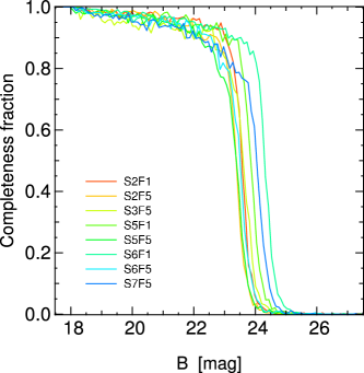
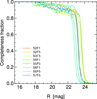
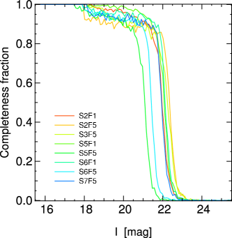
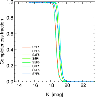
Figure 1: Result of Monte-Carlo completeness simulations with artificial point sources placed in the $B$ (upper left-hand panel), $R$ (upper right-hand panel), $I$ (lower left-hand panel), and $K$-band images (lower right-hand panel) of MUNICS.

In the middle of the 1990s, the $I$-band selected Canada–France Redshift Survey (CFRS) marked an important point in the study of galaxy evolution with redshift surveys. The selection in the $I$ band made it possible to study the evolution of the evolved, massive galaxies rather than star forming galaxies picked up in the more traditional $B$-band selected samples. The CFRS comprises spectra of more than 1000 objects with $17.5\leq I_{AB}\leq 22.5$, 591 of which are galaxies with secure redshifts in the range $0\leq z\leq 1.3$ and enabled studies of the evolution of the luminosity function (Lilly et al., 1995) and of the luminosity density and star formation rate density of the universe (Lilly et al., 1996), finding very little evolution in the luminosity and number density of red galaxies in the redshift range $0<z<1$.

Selection in near-infrared filters like the $K$-band comes even closer to a selection in stellar mass. When suitable near-infrared detectors became available at large telescopes, a number of $K$-band selected surveys were undertaken which can probe the evolution of massive galaxies out to redshift $z\;\sim\;1$. Examples for such surveys are the Hawaii Deep Fields (Cowie et al., 1994), the K20 Survey (Cimatti et al., 2002) and the Munich Near-Infrared Cluster Survey (MUNICS; Drory et al. 2001b).

In this paper we present $B$, $R$, and $I$ band selected MUNICS catalogues which can be used for comparison with previous work and, together with the $K$-band selected catalogue, to study selection effects in extra-galactic surveys. They are an important tool to trace different parts of the field galaxy population, and to discriminate between selection biases and real evolutionary effects. Furthermore, this paper also serves as a general update to Drory et al. (2001b). Since the publication of that paper, the survey’s high-quality multi-colour imaging part has not only grown in area, but $B$-band imaging has become available, and the catalogue has been improved in a number of ways.

This paper is organised as follows. Section 2 gives a brief overview of the Munich Near-Infrared Cluster Survey (MUNICS), while Section 3 describes the construction and content of the optically selected catalogues presented in this paper. In Section 4 we present galaxy number counts in all six filters and compare them to previous studies. Section 5 discusses results on the rest-frame colour distributions of galaxies in the different catalogues, Sections 6 and 7 elaborate on the influence of selection effects and environment on the SSFR, respectively, while Section 8 presents results on the evolution of luminosity functions, before we summarise our findings in Section 9. Throughout this work we assume $\Omega_{M}=0.3$, $\Omega_{\Lambda}=0.7$ and $H_{0}=70\,\mathrm{km}\,\mathrm{s}^{-1}\,\mathrm{Mpc}^{-1}$. All magnitudes are given in the Vega system.

Table 1: The ten MUNICS fields. The table gives the field name, the field coordinates (right ascension $\alpha$ and declination $\delta$ as well as galactic coordinates $l$ and $b$) for the equinox 2000.0 and the effective area of the field in square arc-minutes. The effective area is the area of the sky covered by observations in all six filters.

Field	$\alpha$	$\delta$	$l$	$b$	Area
	(2000.0)		(2000.0)		[arcmin2]
S2F1	03:06:41	$+$00:01:12	178.66	$-$47.67	119.1
S2F5	03:06:41	$-$00:13:30	178.93	$-$47.84	123.7
S3F1	09:04:38	$+$30:02:56	195.37	$+$40.64	116.6
S3F5	09:03:44	$+$30:02:56	195.32	$+$40.45	107.6
S4F1	03:15:00	$+$00:07:41	180.58	$-$46.05	105.6
S5F1	10:24:01	$+$39:46:37	180.85	$+$57.04	115.7
S5F5	10:25:14	$+$39:46:37	180.76	$+$57.27	105.3
S6F1	11:55:58	$+$65:35:55	131.90	$+$50.55	117.1
S6F5	11:57:56	$+$65:35:55	131.60	$+$50.62	116.5
S7F5	13:34:44	$+$16:51:44	349.45	$+$75.66	119.1
All					1146.3

2 The Munich Near-Infrared Cluster Survey (MUNICS)

The Munich Near-Infrared Cluster Survey (or MUNICS for short) is a wide-field medium-deep imaging survey in the near-infrared and optical initially described in Drory et al. (2001b). Dedicated follow-up spectroscopy is available for $\sim 600$ galaxies (Feulner et al., 2003). The main part of the survey consists of 10 fields the details of which are summarised in Table 1. For all these fields photometry in $K^{\prime}$, $J$, $I$, $R$, $V$, and $B$ is available, with limiting magnitudes ranging from $K^{\prime}\simeq 19.5$ to $B\simeq 24.5$ (50% completeness for point sources; Snigula et al. 2002). The total area of this part of the survey is 1146.3 square arcmin (or 0.32 square degrees). However, the fields S3F1 and S4F1 have less than satisfactory quality, especially concerning their photometric calibration. Since an accurate calibration of photometric colours is essential for high-quality photometric redshifts, we exclude these two fields from any further analysis (as has been done with the $K$-selected sample). The total area of the eight high-quality fields is then 924.1 square arcmin (or 0.26 square degrees).

Most of the research on field galaxy evolution and galaxy clusters in the MUNICS project has been carried out with the $K$-band selected catalogue presented in Drory et al. (2001b). This includes studies of luminosity function evolution (Feulner et al., 2003; Drory et al., 2003), the stellar mass function of galaxies (Drory et al. 2001a, 2004), the integrated specific star formation rate of groups (Feulner et al., 2006), and the cluster catalogue described in Botzler et al. (2007). Feulner et al. (2005b), however, a study of the evolution of the specific star-formation rate with redshift, is based on the $I$-band selected catalogue. In this paper, the $I$-, $R$-, and $B$-selected MUNICS samples will be described for the first time in detail.

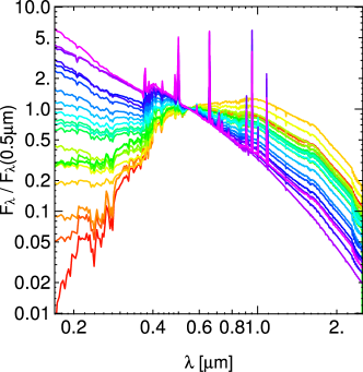
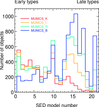
Figure 2: Left-hand panel: Template spectral energy distributions (SEDs) for galaxies used in the computation of photometric redshifts for the $K$-, $I$-, $R$-, and $B$-selected samples. Right-hand panel: The distribution of SED types in the four MUNICS catalogues. The SED number is an internal SED identification: Small numbers refer to redder (early-type) galaxies, higher numbers to bluer (late-type) galaxies.

3 The Construction of Optically Selected Catalogues

In this section we want to discuss the construction and the properties of the $B$, $R$, and $I$-band selected photometric catalogues as well as the measurement and reliability of photometric redshifts. We will often refer to the different catalogues as MUNICS_B, MUNICS_R, MUNICS_I, and MUNICS_K for short.

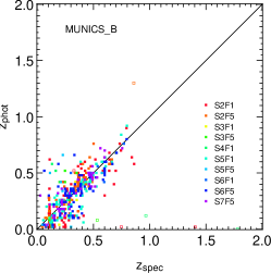
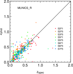
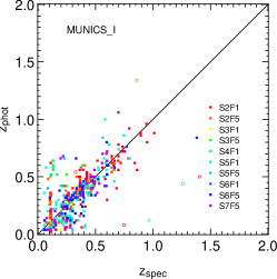
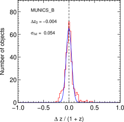
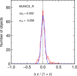
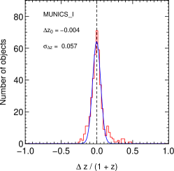
Figure 3: Upper panels: A comparison of photometric and spectroscopic redshifts for MUNICS_B (left), MUNICS_R (middle), and MUNICS_I (right). Filled symbols are galaxies, open symbols quasars. Lower panels: The corresponding histograms of the redshift differences together with a Gaussian fit showing the quality of the photometric redshifts. The corresponding diagrams for MUNICS_K are published in Drory et al. (2003).

3.1 Object Detection

As for the $K$-selected catalogue, object detection on the $B$, $R$, and $I$-band images was performed using the yoda source extraction software (Drory, 2003). Sources are detected by requiring a minimum number $N_{pix}$ of consecutive pixels to lie above a certain threshold $t$ expressed in units of the local RMS $\sigma$ of the background noise. To ensure secure detection of faint sources, the images are convolved with a Gaussian of full width at half maximum (FWHM) similar to the seeing in the image. The choice of the number of consecutive pixels $N_{pix}$ and the threshold $t$ is a compromise between limiting magnitude at some completeness fraction, say 50 per cent, and the number of tolerable spurious detections per unit image area (Saha 1995, see also the discussion in Drory et al. 2001b).

To find reasonable values for $N_{pix}$ and $t$ we performed simulations with varying minimum number of consecutive pixels on the optical images of one of our mosaic fields (S6F5). Instead of fixing two parameters (the threshold and the convolution kernel) and keeping only one free parameter (as with the $K$-band detection), we chose only one fixed parameter: The size of the convolution kernel was set to be equal to the (Gaussian) point-spread function (PSF) of the images. Thus we kept both the threshold and the number of consecutive pixels as free parameters in our simulations. Choosing a PSF-like Gaussian kernel for the image convolution is necessary to ensure secure detection of faint, compact objects in the images. The number of false detections was measured by running the detection algorithm on the same images multiplied by $-1$.

From these simulations, the best choice of parameters is $t=4\sigma$ for the detection threshold, and $N_{pix}=\pi({\mathrm{F}WHM}/2)^{2}$ for the minimum number of consecutive pixels required for an object. With these settings, the contamination rate (the rate of false detections) is actually below 1 per cent.

Since one of the ideas of this paper is a comparison of properties of the $K$-band and the optically selected galaxies, we have convinced ourselves that this change of detection parameters does not influence the results presented here. The reason is that different detection parameter choices mostly affect the object statistics at the very faintest apparent magnitudes. Since these objects also have large photometric errors, they are usually excluded from any further analysis and thus cannot influence the results of our work.

In Figure 1 we show the completeness functions for the $B$, $R$, and $I$-band images of the eight high-quality MUNICS mosaic fields, based on Monte-Carlo simulations of artificial point-sources placed at random in the images. In these simulations, $200$ artificial objects with a Moffat-type PSF having the same FWHM as stars in the frames and a constant magnitude distribution were added to the images using the iraf artdata package. After running the object detection algorithm on the images applying the same detection parameters as for the main catalogue, the fraction of re-detected artificial objects as a function of magnitude is computed. This procedure was repeated $500$ times in order to decrease statistical errors. An extensive discussion of completeness simulations for extended objects in MUNICS $K$-band images can be found in Snigula et al. (2002).

One can see from the diagram that the 50% completeness limits for point sources as derived from these simulations are $B\simeq 24.5$ mag, $R\simeq 23.5$ mag, $I\simeq 22.5$ mag, and $K\simeq 19.5$ mag.

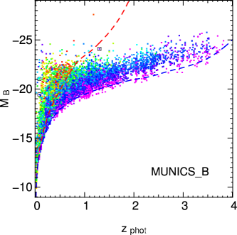
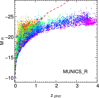
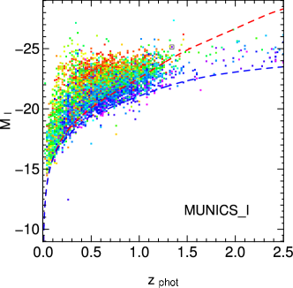
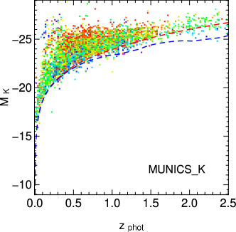
Figure 4: Plots of the absolute magnitudes $M_{B}$, $M_{R}$, $M_{I}$, and $M_{K}$ versus the photometric redshift $z_{\mathrm{phot}}$ for MUNICS_B (upper left-hand panel), MUNICS_R (upper right-hand panel), MUNICS_I (lower left-hand panel) and MUNICS_K (lower right-hand panel), respectively. The different colours denote the different model SEDs, where the colour corresponds roughly to the model colour, i.e. early-type galaxies are shown in red, late-type galaxies in blue. Objects spectroscopically classified as active galactic nuclei (AGN) are additionally marked as open squares. The dashed lines represent the expected absolute magnitudes as a function of redshift for an early-type SED (red dashed line) and a very late type SED (blue dashed line) at the limiting magnitudes of the samples, i.e. $B=24.5$, $R=23.5$, $I=22.5$, and $K^{\prime}=19.5$.

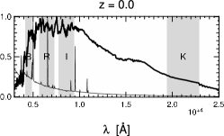
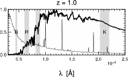
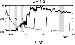
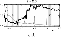
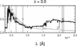
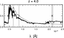
Figure 5: Redshifted spectral energy distributions (arbitrarily normalised) of an early-type galaxy (thick line) and a star-burst galaxy (thin line) and the selection filters $B$, $R$, $I$, and $K$ (shaded areas) for various redshifts. The early-type SED is constructed from Bruzual & Charlot (2003) models and has an age comparable to the age of the universe at each redshift.

3.2 Photometry

Photometry was done in elliptical apertures the shape of which was determined from the first and second moments of the light distribution in the detection image, as described in Drory (2003), and additionally in fixed size circular apertures of 5 and 7 arc seconds diameter. To ensure measurement at equal physical scales in every pass-band, the individual frames were convolved to the same seeing FWHM, namely that of the image with the worst seeing in each field.

Figure 6: Histograms of photometric redshifts for MUNICS_B (dotted line), MUNICS_R (dashed line), MUNICS_I (dot-dashed line), and MUNICS_K (solid line).

Aperture fluxes and magnitudes were computed for each object present in the $B$, $R$, and $I$-band catalogues irrespective of a detection in any other band. For this purpose the centroid coordinates of the sources found in the detection images were transformed to the other frames using geometric transformations between the image coordinate systems. For this purpose, the images in the other five filters of each field were registered against the image in the detection band by matching the positions of $\sim 200$ bright homogeneously distributed objects in the frames and determining the coordinate transform from the detection system to each image in the other five pass-bands using the tasks xyxymatch and geomap within iraf. The scatter in the determined solutions is less than 0.1 pixels RMS in the transformation from $I$ or $B$ to the other optical bands, and less than 0.2 pixels RMS from $I$ or $B$ to the near-infrared frames. Note that the frames themselves are not transformed to avoid artefacts from the re-sampling. We only determine accurate transformations and apply these later to the apertures in the photometry process, where the shapes of the apertures were transformed using only the linear terms of the transformation.

As a result of this method, small differences in object centring and differences in the object’s shape in the different detection images lead to slightly different photometry in the various catalogues. Nevertheless, a direct comparison of magnitudes in the same filter, but derived in the different selection catalogues is an important consistency check. The comparison shows excellent agreement between MUNICS_B, MUNICS_R, MUNICS_I, and MUNICS_K (comparison plots are published in Feulner, 2004).

3.3 Photometric Redshifts

Photometric redshifts are derived using the method presented in Bender et al. (2001), a template matching algorithm rooted in Bayesian statistics closely resembling the method presented by Benítez (2000). The application of this method to the $K$-selected MUNICS sample is described in great detail in Drory et al. (2003).

The left-hand panel of Figure 2 shows the final template spectral energy distribution (SED) library used to derive photometric redshifts in what follows. It is the same set of SEDs also used for the $K$-band selected catalogue, since these SEDs already cover a vast range from very red old models to young star-bursting models. As we show in the right-hand panel of Figure 2, the difference between the differently selected catalogue lies then in the distribution of selected SEDs: While in the $K$-selected sample the algorithm picks preferentially red galaxy types (and only very few heavily star-forming objects), the distribution for the $I$- and $R$-selected samples is more balanced, and indeed reversed for the $B$-selected sample.

Figure 3 compares photometric and spectroscopic redshifts for all $\sim 600$ objects with spectroscopic redshifts within the MUNICS fields and shows the distribution of redshift errors. The typical scatter in the relative redshift error $\Delta z/(1+z)$ is 0.057. This is very similar to the results for the $K$-band selected catalogue described in Drory et al. (2003). The mean redshift bias is negligible. The distribution of the errors is roughly Gaussian. There is no visible difference between the distributions among the survey fields. Although this performance is encouraging, it is important to say that the spectroscopic data become sparse at $z\ga 0.6$ and there are only very few spectroscopic redshifts at $z>1$. Note that many quasars are among the few dramatic outliers which is to be expected from the power-law like SEDs of active galactic nuclei.

Many objects in the MUNICS fields are, of course, detected in more than one band. As a consistency check, we present comparisons of the photometric redshifts of these objects derived in different catalogues in Appendix A, showing excellent agreement.

In Figure 4 we show the distribution of absolute $B$, $R$, $I$, and $K$ magnitude versus photometric redshift for the four MUNICS samples and for different model SEDs, ranging from early types (redder colours) to late types (bluer colours). We also show the expected curve for a early-type model SED (red dashed line) and a very late type model SED (blue dashed line) at the limiting magnitudes of the samples, i.e. $B=24.5$, $R=23.5$, $I=22.5$, and $K^{\prime}=19.5$.

The object distribution is generally in very good agreement with the expectations. Outlying objects with suspiciously high luminosities are likely to be partly photometric-redshift outliers and active galactic nuclei (AGN). Indeed, spectroscopically identified AGN are marked in the Figure, and they are found in this region of the diagram. Note that the spectroscopic follow-up of MUNICS was pre-selected against point sources (see Feulner et al., 2003), and that the existing AGN spectra are mostly drawn from a sample of AGN selected for their red colour (Wisotzki et al., in preparation). The lack of objects with $z\geq 1.5$ in MUNICS_I seems puzzling at first. From their apparent magnitudes we should be able to detect blue galaxies at these redshifts. To investigate this apparent failure, we have selected objects in this redshift range from MUNICS_R and plotted their position in the $I$-band images. It turns out that these objects are simply not detected due to the higher noise level in the $I$-band images caused by fringing. The higher noise level reduces the overall depth of the sample and affects galaxies at all redshift. Looking at this effect in terms of the luminosity function (LF) at different redshifts, the incompleteness cuts away the faint end of the LF in each redshift bin, with the limit moving to higher luminosities with increasing redshift. At redshift $z\sim 1.5$ the $I$-band magnitude limit of MUNICS_I reaches the bright end of the LF, i.e. only very few galaxies in this redshift range are detected. We have verified this by taking the $R$-selected catalogue and plotting that $I$-band magnitude histogram of all galaxies beyond $z=1.5$ which indeed falls below the $I$-band detection limit. Also, the much deeper $I$-selected FDF catalogue (Heidt et al., 2003) cut at the MUNICS_I limit shows a redshift distribution similar to the one for MUNICS_I. Note that this lack of galaxies beyond $z\sim 1.5$ in the $I$-selected sample does not cause any problems as long as one excludes these higher redshifts from any analysis.

The distribution of SED types in Figure 4 clearly illustrates the importance of selection effects at higher redshift: While the $K$-selected sample traces the population of early-type galaxies out to redshifts beyond $z\simeq 1.5$ (at the limiting magnitudes of MUNICS; indeed, that is how the survey was designed), it lacks late-type galaxies at all redshifts. The $B$-selected sample on the other hand does not contain early-type galaxies beyond $z\simeq 0.8$ (again at the limiting magnitudes of MUNICS), but is much better suited for tracing late-type galaxies at low and high redshift.

These selection effects can be easily understood by looking at the position of redshifted SEDs with respect to the four detection filters as shown in Figure 5 where we plot redshifted SEDs for an early-type and a star-burst galaxy. Early-type galaxies disappear from a $B$-selected catalogue at $z\sim 1$ and from $R$ as well as $I$-selected catalogues at $z\sim 1.5$, while they remain visible to much higher redshifts in MUNICS_K. Similarly, the detection of very blue galaxies at redshifts $z\sim 3$ in MUNICS_B and MUNICS_R can be explained by the strong rest-frame ultraviolet emission at wavelengths longer than that of the Lyman break entering the detection bands.

The photometric redshift histograms for MUNICS_B, MUNICS_R, MUNICS_I, and MUNICS_K can be found in Figure 6. Note the high redshift tails in the distributions for MUNICS_B, MUNICS_R, and MUNICS_K, caused by luminous red galaxies at $1\;\la\;z\;\la\;2$ and the ultraviolet emission of blue galaxies shifted into the optical bands, respectively.

3.4 Star–Galaxy Separation

For computing statistical properties of the field-galaxy population like its luminosity function, it is necessary to remove all stars from the analysis. In a photometric catalogue, this can be done in two ways. Either by looking at an object’s morphology in the image, i.e. whether it appears to be similar to the point-spread function (PSF) of the image or extended, or by looking at the spectral energy distribution (SED), in this case as traced by the six-filter photometry, and comparing it to template spectra of stars and galaxies. The disadvantage of the morphological approach is clearly its tendency to fail at fainter magnitudes (because of the lower signal-to-noise ratio and because distant galaxies look more and more compact), while it works reasonably well at brighter magnitudes (see, e.g., Drory et al. 2001b).

For this investigation, we decided to take the second route. The photometric redshift technique as described above compares the photometry in the six MUNICS filters to template SEDs of stars and galaxies. Each fit is assigned a $\chi^{2}$ value, and we can simply discriminate between stars and galaxies by comparing the $\chi^{2}$ values of the best-fitting stellar and the best-fitting galactic SED. More specifically, we classify all objects as stars for which $\chi^{2}_{\mathrm{star}}<\chi^{2}_{\mathrm{galaxy}}$.

This procedure can be tested by checking against the spectroscopic sample described in Feulner et al. (2003). This is illustrated in Figure 7, where we show the $\chi^{2}$ values of objects spectroscopically classified as stars or galaxies, respectively, for the $B$-selected catalogue. The diagrams for the other samples are very similar. Clearly, the SED classifier does work very well. Note that in all comparisons between MUNICS_B, MUNICS_R, MUNICS_I, and MUNICS_K presented in this paper we have used the same $\chi^{2}$-based classification method.

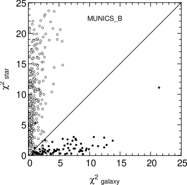
Figure 7: This diagram shows the loci of spectroscopically classified galaxies (open circles) and stars (crosses) in a plane defined by the $\chi^{2}$ values of the best-fitting galactic and stellar spectral-energy distributions (SEDs) for MUNICS_B. The line used to discriminate the two classes is also indicated. The corresponding diagrams for MUNICS_R, MUNICS_I, and MUNICS_K look very similar.

4 Galaxy Number Counts

Galaxy number counts, although not as widely accepted as important tool for the study of galaxy evolution and cosmology as in the past, still serve as an interesting probe of a survey’s data quality. Since the publication of galaxy number counts from MUNICS in Drory et al. (2001b), the survey has considerably increased in size and quality. Moreover, $B$-band number counts have never been published for the MUNICS project, so we show galaxy number counts in all six filters $B$, $V$, $R$, $I$, $J$ and $K$ in Figure 8. The counts were derived from detection catalogues constructed on all filter images. In contrast to the analysis presented later in this paper, star–galaxy separation is based on the morphological classifier described in detail in Drory et al. (2001b). The reason for this is that no photometric redshift data are available for the $V$, $R$ and $J$-band detections, so we cannot rely on the $\chi^{2}$-based classification. However, the two classification methods agree very well. Completeness-corrected galaxy number counts from MUNICS are presented here for the first time. The completeness correction is based on the simulations described in Section 3.1. All errors given are Poissonian errors.

The galaxy number counts presented in Figure 8 for all six MUNICS filters show excellent agreement with existing data and clearly demonstrate the quality of our dataset. The completeness-corrected values for the number counts are also summarised in Table 2.

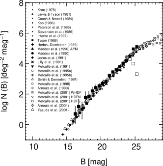
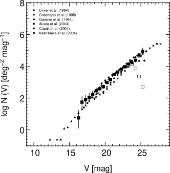
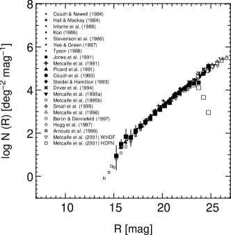
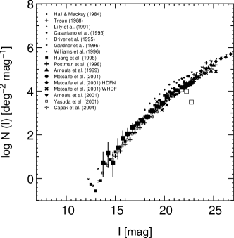
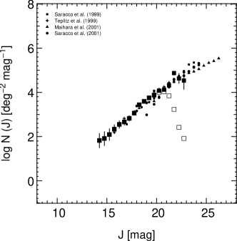
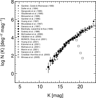
Figure 8: Galaxy number counts from MUNICS (large squares) in $B$ (upper left-hand panel), $V$ (upper right-hand panel), $R$ (middle left-hand panel), $I$ (middle right-hand panel), $J$ (lower left-hand panel) and $K$ (lower right-hand panel). The filled squares indicated completeness-corrected counts, whereas the open squares represent the uncorrected values. Literature counts are shown for comparison.

Table 2: Completeness corrected galaxy number counts from MUNICS in the $B$, $V$, $R$, $I$, $J$ and $K$ bands. $\log N$ and $\sigma_{\log N}$ are given, where $N$ is in units of $\mathrm{mag}^{-1}\mathrm{deg}^{-2}$.

	$B$		$V$		$R$		$I$		$J$		$K$
$m$	$\log N$	$\sigma_{\log N}$	$\log N$	$\sigma_{\log N}$	$\log N$	$\sigma_{\log N}$	$\log N$	$\sigma_{\log N}$	$\log N$	$\sigma_{\log N}$	$\log N$	$\sigma_{\log N}$
12.25											0.72	0.60
12.75											1.41	0.51
13.25											1.41	0.42
13.75											1.92	0.33
14.25							1.18	0.60	1.82	0.34	2.05	0.32
14.75							0.73	0.60	1.91	0.33	2.46	0.19
15.25					0.95	0.60	1.41	0.51	2.09	0.28	2.54	0.17
15.75					1.49	0.23	1.85	0.37	2.33	0.21	2.75	0.13
16.25	0.71	0.60	0.75	0.60	1.84	0.39	2.05	0.26	2.55	0.17	3.25	0.07
16.75	1.18	0.60	1.74	0.41	1.80	0.41	2.35	0.21	2.67	0.14	3.44	0.05
17.25	1.00	0.60	1.90	0.30	2.11	0.28	2.52	0.17	2.82	0.12	3.61	0.04
17.75	1.78	0.45	2.03	0.32	2.34	0.20	2.68	0.14	3.06	0.09	3.74	0.04
18.25	1.85	0.37	2.22	0.23	2.52	0.17	2.83	0.11	3.44	0.05	3.89	0.03
18.75	2.21	0.27	2.47	0.18	2.69	0.13	3.11	0.08	3.59	0.04	3.96	0.03
19.25	2.42	0.19	2.59	0.15	2.91	0.10	3.29	0.06	3.75	0.04	4.05	0.05
19.75	2.53	0.17	2.72	0.13	3.10	0.08	3.44	0.05	3.88	0.03	4.32	0.14
20.25	2.70	0.14	2.98	0.09	3.26	0.06	3.75	0.04	4.08	0.03	4.53	0.26
20.75	2.82	0.12	3.16	0.07	3.42	0.05	3.90	0.03	4.12	0.03	4.75	0.25
21.25	3.22	0.07	3.49	0.05	3.73	0.04	4.04	0.03	4.32	0.03
21.75	3.45	0.05	3.64	0.04	3.87	0.03	4.17	0.03	4.87	0.06
22.25	3.59	0.04	3.83	0.03	4.05	0.03	4.29	0.06	4.63	0.23
22.75	3.79	0.03	3.99	0.03	4.21	0.02	4.39	0.14
23.25	4.02	0.03	4.15	0.02	4.30	0.02
23.75	4.20	0.02	4.23	0.03	4.34	0.03
24.25	4.49	0.02	4.39	0.06	4.77	0.06
24.75	4.97	0.03	4.72	0.08	5.11	0.12
25.25	5.12	0.07	4.95	0.21

Figure 9: Distribution of rest-frame $B-K$ colours as a function of selection band, luminosity, and redshift. Upper left-hand panel: All galaxies with $0\leq z\leq 1$ in the $K$-band selected (solid line), $I$-band selected (dot-dashed line), $R$-band selected (dashed line) and $B$-band selected (dotted line) MUNICS samples, divided into three different $K$-band luminosity classes. All other panels: Sub-divided into galaxies with $0\leq z\leq 0.5$ (dashed line) and $0.5\leq z\leq 1.0$ (dotted line) for MUNICS_B (upper right-hand panel), MUNICS_R (lower left-hand panel), and MUNICS_K (lower right-hand panel). In each plot, the distribution of Poisson errors is also shown below the object histograms. Furthermore, typical $B-K$ error bars are also indicated in every plot.

5 Distribution of Rest-Frame Colours

In this paper, we want to investigate the differences of the galaxy populations in $K$, $I$, $R$, and $B$-selected samples and follow their evolution with redshift. One simple, but rewarding way of doing this is to study rest-frame colour distributions as a function of luminosity and redshift. Cole et al. (2001) divided their $K$-selected sample of local galaxies into three luminosity classes and looked at the distribution of rest-frame $b_{J}-K_{\mathrm{s}}$ and $J-K_{\mathrm{s}}$ colours. Since the $K$-band luminosity is a measure of a galaxy’s stellar mass, the luminosity classes correspond to a binning in stellar mass. Their main finding is that at smaller $K$-luminosities (i.e. smaller masses) there is a more and more prominent population of blue, star forming galaxies. It is interesting to test this also for higher redshifts and different selection bands.

The solid line in the upper left-hand panel of Figure 9 shows the $B-K$ rest-frame colour distributions of $K$-selected MUNICS galaxies at $0\leq z\leq 1$, confirming the result of Cole et al. (2001). Moreover, we present in this Figure the same distributions for $I$-band (dot-dashed line) as well as $R$-band selected MUNICS galaxies (dashed line), showing clearly that the main difference between near-infrared and optically selected samples are the bluer colours of low-luminosity (low-mass) galaxies. This is even more pronounced for the $B$-selected sample shown as a dotted line.

Four conclusions can be immediately drawn from this distributions. Firstly, as already noted by Cole et al. (2001), a population of blue, star forming galaxies contributes more strongly at fainter luminosities. Secondly, this populations becomes more numerous at bluer selection wavelengths. Thirdly, the colour distribution seems to be wider at fainter absolute $K$-band magnitudes (although part of this effect may be attributed to the larger errors in the rest-frame $B-K$ colour for these objects). Fourthly, and maybe most importantly, the colour distributions of high-mass galaxies change very little as a function of redshift. Hence one would not expect much variation of the bright end of the galaxy luminosity function in different selection bands like $K$ and $I$. The faint end, however, will be certainly affected in the sense that in bluer selection bands the faint-end slope will likely be steeper.

In the other three panels of Figure 9 we present the rest-frame $B-K$ colour distributions in the two redshift intervals $[0.0,0.5]$ and $[0.5,1.0]$ for MUNICS_B (upper right-hand panel), MUNICS_R (lower left-hand panel) and MUNICS_K (lower right-hand panel). First, it is very interesting that the colour distributions agree so well for the highest luminosity objects (irrespective of the selection filter). Furthermore, there is a clear trend with redshift in the sense that lower-luminosity objects get bluer. That means that even at redshift $z\sim 1$ the increased star-formation rate is dominated by low-luminosity (low-mass) systems. Finally, it is worth noting that this evolutionary trend with redshift is barely visible in the $K$-selected sample, clearly evident in the $R$-selected sample, but gets very large in the $B$-selected sample: Indeed, for the low-mass objects with $-21.75\;>\;M_{K}\;>\;-23.00$, the shift between redshift $z\;\sim\;0.25$ and $z\;\sim\;0.75$ is $\Delta(B-K)\sim 0.3$ for MUNICS_K, $\Delta(B-K)\sim 0.7$ for MUNICS_R, but as large as $\Delta(B-K)\sim 1.0$ for MUNICS_B.

How can this be interpreted? The rest-frame colour of a galaxy is governed by the age of its stellar population, its star-formation activity, the metalicity and the dust content. Let us neglect the influence of metalicity and dust for the moment. The lack of redshift evolution of the rest-frame colours of high $K$-band luminosity galaxies over $0\;\la\;z\;\la\;1$ means that these objects must have built up their stellar mass at earlier times. The fact that also at lower $K$ luminosities galaxies of similar rest-frame colour can be found even in the higher redshift bin indicates that also part of the lower mass objects formed early, although the majority of them had (or has) major star-formation activity at $z\;\la\;1$. It is also clear from these colour distributions that the rise of the star-formation rate to redshift unity is mostly driven by lower-mass galaxies. Note that ‘lower mass’ in this context includes intermediate-mass spirals for which there is evidence for increased star-formation activity in the past (Bell et al., 2005).

Overall, this picture of different paths of evolution for the most massive and the lower-mass galaxies is in good agreement with recent findings on the evolution of the specific star-formation rate (SSFR), i.e. the star formation rate per unit stellar mass (see, e.g., Feulner et al. 2005a and references therein). We will discuss the SSFR in more detail in Sections 6 and 7 of this paper.

6 The Specific Star Formation Rate and Selection Effects

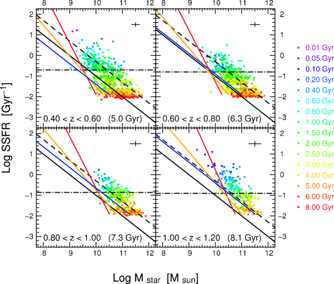
Figure 10: SSFR versus stellar mass for galaxies in MUNICS_K (symbols). Objects are coloured according to the age of the composite stellar-population synthesis model fit to their photometry, ranging from 0.01 Gyr (purple) to 8 Gyr (red). The solid and dashed black lines correspond to SFRs of $1\;M_{\odot}\;\mathrm{yr}^{-1}$ and $5\;M_{\odot}\;\mathrm{yr}^{-1}$, respectively. The dot-dashed line is the SSFR required to double a galaxy’s mass between each redshift epoch and today, assuming constant SFR. The corresponding look-back time as well as an estimate of the typical error bars are indicated in each panel. Selection effects in this diagram are visualised for MUNICS_K (red line), MUNICS_I (orange line), and MUNICS_B (blue line).

In this Section we will discuss the influence of the selection band on the specific star formation rate (SSFR), i.e. the star formation rate per unit stellar mass.

As in Feulner et al. (2005b), we estimate the star formation rates (SFRs) of our galaxies from the SEDs by deriving the luminosity at $\lambda=2800\pm 100$Å and converting it to an SFR as described in Madau et al. (1998) assuming a Salpeter initial mass function (IMF; Salpeter 1955). We have convinced ourselves that these photometrically derived SFRs are in reasonable agreement with spectroscopic indicators for objects with available spectroscopy. Note that since our bluest band is $B$, this is an extrapolation for $z<0.4$. Hence we restrict any further analysis to redshifts $z>0.4$, where the ultraviolet continuum at $\lambda\simeq 2800$Å is shifted into or beyond the $B$ band.

Stellar masses are computed from the multi-colour photometry using a method similar to the one used in Drory et al. (2004). It is described in detail and tested against spectroscopic and dynamical mass estimates in Drory, Bender & Hopp (2004). In brief, we derive stellar masses by fitting a grid of stellar population synthesis models by Bruzual & Charlot (2003) with a range of star formation histories (SFHs), ages, metalicities and dust attenuations to the broad-band photometry. We describe star formation histories (SFHs) by a two-component model consisting of a main component with a smooth SFH $\propto\exp(-t/\tau)$ and a burst. We allow SFH time-scales $\tau\in[0.1,\infty]$ Gyr, metalicities $[\mathrm{Fe/H}]\in[-0.6,0.3]$, ages between 0.5 Gyr and the age of the universe at the objects redshift, and extinctions $A_{V}\in[0,1.5]$. The SFRs derived from this model fitting is in good agreement with the ones from the ultraviolet continuum. Note that we apply the extinction correction derived from this fitting also to the SFRs.

Figure 10 presents the SSFR versus stellar mass diagram for four redshift bins as derived from MUNICS_K. The influence of the limiting apparent magnitude of the $K$-selected catalogue is clearly visible in the lower left-hand part of the panels. The boundary for MUNICS_K is marked by the red solid line, while the orange and blue lines give the limits of the point distributions for MUNICS_I and MUNICS_B, respectively.

The selection band clearly affects the slope of this boundary. While for the $K$-selected catalogue the line is steeper (i.e. closer to a selection in stellar mass), it gets gradually shallower for selection bands at shorter wavelengths. For MUNICS_B, the ridge runs essentially parallel to lines of constant SFR, demonstrating that $B$-band selection indeed selects galaxies according to their star-formation activity.

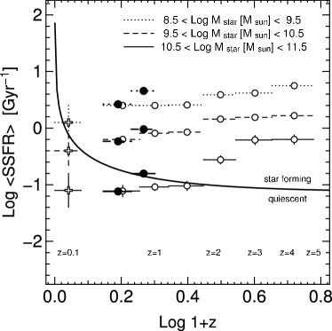
Figure 11: The average SSFR of galaxies in three mass intervals (see legend) as a function of redshift for galaxies in MUNICS_B (filled circles), FDF/GOODS-S (open circles; Feulner et al. 2005), and SDSS (open crosses; Brinchmann et al. 2004).

For massive galaxies ($\log M_{\ast}>9.5$) with non-negligible star-formation activity ($\mathrm{SFR}\;>\;1\;M_{\odot}\;\mathrm{yr}^{-1}$) at redshifts $z<1$ there is little difference between the three selection bands. This can also be seen in Figure 11 where we compare the average SSFR as a function of redshift for galaxies in three different mass bins as derived from MUNICS_B and a combined sample from the $I$-selected FDF, and the $K$-selected GOODS catalogue (Feulner et al., 2005). We chose MUNICS_B for this exercise because it is the only sample not affected by incompleteness for the lowest mass bin. Values from MUNICS_B and FDF/GOODS-S are in remarkable agreement. The good agreement between the $I$-selected FDF and the $K$-selected GOODS-S catalogue has already been demonstrated in Feulner et al. (2005a). We also show local values as derived by Brinchmann et al. (2004) for the Sloan Digital Sky Survey (SDSS). We have shifted these by $\Delta\mathrm{SSFR}\>=\>+0.6$ to account for differences in the normalisation of the SFR and in the dust correction.

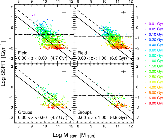
Figure 12: SSFR versus stellar mass for galaxies in MUNICS_K (symbols) for field galaxies (upper panels) and galaxies in MUNICS groups (lower panels). See caption of Figure 10 for details.

7 The Specific Star Formation Rate in Different Environments

To study the influence of the environment on the SSFRs of galaxies we investigate its behaviour for field galaxies and for galaxies in groups. Group membership in the $K$-selected MUNICS catalogue is assigned according to a modified version of the friends-of-friends algorithm, specifically designed to cope with photometric redshift datasets (Botzler et al., 2004). In brief, the algorithm works in redshift slices, and corresponding structures in adjacent slices are combined a posteriori. Additionally to the traditional linking parameters in projected distance ($D_{L}$) and velocity space ($V_{L}$), a redshift pre-selection is performed to exclude objects with large photometric redshift errors. The linking criteria used for the MUNICS sample are $D_{L}=0.125\,h^{-1}\,\mathrm{Mpc}$ and $V_{L}=1000\,\mathrm{km\,s}^{-1}$; a minimum number of 3 objects is required to form a group or cluster (Botzler et al., 2007). Expected completeness fractions and contamination rates are roughly 90 per cent and 40 per cent, respectively.

The resulting structure catalogue is presented in Botzler (2004) and Botzler et al. (2007) and comprises 162 structures (mostly groups) containing 890 galaxies in total. This group sample has already been used to study the integrated SSFR of groups in comparison with field galaxies and clusters (Feulner et al., 2006).

A comparison of field galaxies and group members in the SSFR–stellar mass plane in two redshift intervals is presented in Figure 12. In contrast to the field population, group galaxies tend to populate the region of passive galaxies below the doubling line only. This, of course, is in agreement with previous findings that galaxies in higher density environments tend to have lower star-formation activity. Interestingly, however, passive galaxies are by no means limited to the group environment. This could be partially explained by group selection effects, but is in agreement with recent findings by Gerke et al. (2007) who identified a significant population of red galaxies in the field, with morphologies characteristic for passive galaxies.

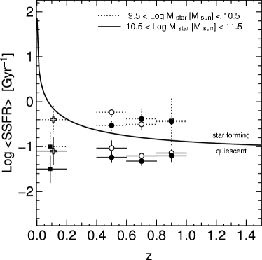
Figure 13: Same as Figure 11 but for MUNICS field galaxies (open circles) and group members (filled circles). The local comparison values are taken from Weinmann et al. (2006) for SDSS groups (filled squares) and from Brinchmann et al. (2004) for SDSS field galaxies (open crosses).

This behaviour is also obvious from Figure 13 where we show the redshift evolution of the average SSFR of galaxies in two different mass intervals, comparing field and group galaxies. At $z\sim 1$ there seems to be no marked difference between field galaxies and galaxies in groups, with a tendency of the difference increasing with decreasing redshift in the sense that group galaxies are rather more inactive than field galaxies. Note that this difference is larger for less massive galaxies than for the most massive objects. This is in principal agreement with earlier findings on the dependence of SSFR on density for galaxies in the local universe (Kauffmann et al., 2004).

The fact that we do not see a more pronounced difference between field and groups could be at least partially attributed to two effects. First, incompleteness of the group catalogue as well as contamination with false structures is likely to reduce the signal. Secondly, trends of the photometric redshift errors with SFR and redshift might affect the analysis, especially in the higher redshift bins. Photometric redshift errors in the MUNICS catalogue increase with redshift (from $\sim 0.08$ at $z=0.5$ to $\sim 0.12$ at $z=1$) and with SFR (they are typically 20 per cent larger for star-forming galaxies as compared to passive galaxies). In reality, the difference in SSFR between groups and the field may be more significant.

8 Evolution of the Luminosity Function

8.1 Computing the Galaxy Luminosity Function

As for the near-infrared luminosity function (LF) presented in Feulner et al. (2003) and Drory et al. (2003), the LF is computed using the non-parametric $V_{\mathrm{max}}$ formalism (Schmidt, 1968). In brief, the $V_{\mathrm{max}}$ formalism accounts for the fact that some fainter galaxies are not visible in the whole survey volume. In a volume-limited redshift survey, each galaxy $i$ in a given redshift bin $[z_{\mathrm{lower}},z_{\mathrm{upper}}]$ contributes to the number density an amount inversely proportional to the volume $V_{i}$ of the survey:

$$V_{i}\;=\;\int\limits_{z_{\mathrm{lower}}}^{z_{\mathrm{upper}}}\>\frac{dV}{dz}\>dz,$$ (1)

where $dV=d\Omega\,r^{2}\,dr$ is the co-moving volume element and $d\Omega$ is the solid angle covered by the survey. However, due to the fact that we have to deal with magnitude-limited surveys, a faint galaxy may not be visible in the whole survey volume. Assuming that in a survey with given limiting magnitude galaxy $i$ can be seen out to redshift $z_{\mathrm{max}}$, we have to correct the volume factor by $V_{i}^{\mathrm{max}}/V_{i}$, where

$$V_{i}^{\mathrm{max}}\;=\;\int\limits_{z_{\mathrm{lower}}}^{\mathrm{min}(z_{\mathrm{upper}},z_{\mathrm{max}})}\>\frac{dV}{dz}\>dz.$$ (2)

Obviously, we have $z_{\mathrm{max}}\geq z_{\mathrm{upper}}$ for a galaxy which is bright enough to be seen in the whole volume in investigation, and the correction factor is one. Otherwise, $z_{\mathrm{max}}<z_{\mathrm{upper}}$, and the volume is smaller than the volume corresponding to the redshift range in which we compute the LF. We have made sure that the effect of the volume correction is of importance only in the faintest bin in absolute magnitude, and that even in this case the correction is at most a factor of 5.

Additionally, the contribution of each galaxy $i$ is weighted by the inverse of the detection probability $P(m_{\mathrm{det},i})$ of the parent catalogue. The LF $\Phi(M)$ is then computed according to the formula

$$\Phi(M)\>dM\;=\;\sum\limits_{i}\>\frac{V_{i}}{V_{i}^{\mathrm{max}}}\>\>\frac{1}{V_{i}}\>\frac{1}{P(m_{\mathrm{det},i})}\>dM,$$ (3)

where the sum runs over all objects $i$ in the redshift range for which we want to calculate the LF. Naturally the volume terms can be simplified to $1/V_{i}^{\mathrm{max}}$.

We include two effects in the total error budget of the luminosity function. Firstly, the limited number of objects in each magnitude bin produces statistical uncertainties. Secondly, the errors in the photometric redshift estimates have some influence on the luminosity function.

The statistical errors are derived using Poissonian statistics, following the methods described in Gehrels (1986), Ebeling (2003), and Ebeling (2004) for approximation of Poissonian errors for small numbers.

To investigate the influence of photometric redshift errors on the luminosity function, we perform Monte-Carlo simulations. In these simulations, we take the original input catalogue used for deriving the luminosity function, and assign to each object a redshift within the redshift error distribution given by the photometric-redshift algorithm. In principle, there are two ways of doing this. Either one uses the redshift probability distribution of the best-fitting SED, or the sum of the probability distributions of all SEDs (the total probability distribution). One might expect the total probability distribution to have the advantage that it accounts better for systematic uncertainties in the SED fitting. However, we have carried out careful tests which show that the errors derived from the total distribution are not significantly different from the ones for the best distribution. This is due to the fact that the probability distribution for the best-fitting SED usually dominates the total distribution. Since the total distribution also takes more Monte-Carlo realisations to converge, we decided to use the probability distribution of the best-fitting SED for our simulations. The median of the redshift error assigned by the photometric redshift algorithm to galaxies in MUNICS_R is $\langle\sigma\rangle_{\mathrm{median}}\simeq 0.08$, in good agreement with the measured deviation of photometric and spectroscopic redshifts of $\delta z/(1+z)\simeq 0.057$. Hence these error distributions are a good representation of the true error distribution.

The errors are then computed as follows. The Poisson error and the standard deviation around the mean derived from the Monte-Carlo simulations are summed quadratically. In addition, any difference between the measured value for the LF in a magnitude bin and the mean from the Monte-Carlo simulations is considered a measure of systematic errors. This is also added quadratically, but only in one direction, i.e. if the Monte-Carlo mean is higher than the measured value the upper error bar is enlarged, but not the lower one. All our $\chi^{2}$ fitting routines, both for the Schechter parameters and for the LF evolution, can handle asymmetric errors.

Figure 14: The $B$-band LF from the $R$-selected catalogue at redshifts $z=0.50$ (upper left-hand panel), $z=0.75$ (upper right-hand panel), $z=1.20$ (lower left-hand panel) and $z=2.00$ (lower right-hand panel). One can clearly see the effect of brightening and decreasing number density with increasing redshift $z$. The local $B$-band LF from Driver et al. (2005) is shown as dotted line, the FDF LF from Gabasch et al. (2004) in the redshift bins [0.45,0.81], [0.45,0.81], [0.81,1.11] and [2.15,2.91] as dashed line.

Figure 15: The $R$-band LF from the $R$-selected catalogue at redshifts $z=0.50$ (upper left-hand panel), $z=0.75$ (upper right-hand panel), $z=1.20$ (lower left-hand panel) and $z=2.00$ (lower right-hand panel). One can clearly see the effect of brightening and decreasing number density with increasing redshift $z$. The local $r^{\prime}$-band LF from Blanton et al. (2003, transformed to the $R$ band) is shown as dotted line, the FDF $r$-band LF from Gabasch et al. (2006, transformed to the $R$ band) in the redshift bins [0.45,0.85], [0.45,0.85], [0.85,1.31] and [1.91,2.61] as dashed line.

8.2 $R$-Band Selected Luminosity Functions

In this Section we present luminosity functions from the $R$-selected MUNICS sample in the redshift intervals $[0.4,0.6]$, $[0.6,0.9]$, $[0.9,1.5]$, and $[1.5,2.5]$. The luminosity function results together with a Schechter approximation (Schechter, 1976) and a local comparison function are presented in Figure 14 for the $B$ band and in Figure 15 for the $R$ band, respectively. We also compare our results to the LF derived in the FDF in Gabasch et al. (2004); Gabasch et al. (2006). The agreement is very good in general, although we see a slight excess of very bright galaxies in MUNICS, resulting in somewhat larger characteristic luminosities and, because of the degeneracy of the Schechter paramters $\Phi^{*}$ and $M^{*}$, lower characteristic densities. The excess of bright galaxies might be caused by three effects. First, quasars which cannot be easily discarded from our photometric catalogue are expected to populate the bright end of the LF (e.g. Jahnke & Wisotzki, 2003). Secondly, a slight excess of bright galaxies as compared to the Schechter function has been noted in spectroscopic surveys in the local universe (e.g. Blanton et al., 2003; Jones et al., 2006). Finally, it may be at least partially attributed to photometric redshift errors s (see, e.g., the simulations in Drory et al., 2003), although in this case the error bars at the bright end of the LF seem to be smaller than the true errors which might point to an underestimation of the errors for individual galaxies, although they are in good agreement with the measured errors on average. In the highest redshift bin, the MUNICS data do not sample the knee of the LF very well, resulting in rather low values for $\Phi^{*}$.

Table 3: Schechter parameters $\Phi^{*}$ and $M^{*}$ and $\alpha$ for the LFs in the $B$ and $R$ band derived from MUNICS_R.

Band	$\langle z\rangle$	$\Phi^{*}$	$M^{*}$	$\alpha$	$M_{\mathrm{lim}}$	$\min(\chi^{2}_{\mathrm{red}})$
		[$10^{-3}$ Mpc-3]	[mag]		[mag]
$B$	0.50	$4.20\pm 0.60$	$-21.39\pm 0.18$	$-1.25$	$-18.0$	$0.37$
	0.75	$3.12\pm 1.08$	$-21.47\pm 0.25$	$-1.25$	$-20.5$	$1.11$
	1.20	$2.32\pm 1.28$	$-21.74\pm 0.29$	$-1.25$	$-20.5$	$0.28$
	2.00	$0.68\pm 0.22$	$-22.86\pm 0.22$	$-1.25$	$-22.0$	$0.41$
$R$	0.50	$2.96\pm 0.36$	$-22.64\pm 0.18$	$-1.33$	$-18.0$	$0.37$
	0.75	$3.12\pm 0.62$	$-22.54\pm 0.18$	$-1.33$	$-20.0$	$0.58$
	1.20	$1.16\pm 0.60$	$-23.18\pm 0.30$	$-1.33$	$-21.5$	$0.28$
	2.00	$0.72\pm 0.30$	$-23.66\pm 0.26$	$-1.33$	$-23.0$	$0.22$

We summarise the parameters $\Phi^{*}$, $M^{*}$ and $\alpha$ of the Schechter fits in Table 3 and show the corresponding Schechter contours in Figure 16. Note that we have kept the faint-end slope $\alpha$ fixed to the value $-1.25$ ($B$ band) and $-1.33$ ($R$ band) during the fitting process. These are the values derived for the FDF in Gabasch et al. (2004) and Gabasch et al. (2006), respectively, which are in good agreement with the MUNICS LFs in the lowest redshift bin. At higher redshifts, the MUNICS data are not sufficiently deep to constrain the faint-end slope.

Figure 16: Schechter contours in the $\Phi^{*}$–$M^{*}$ plane for the $B$-band LF (left-hand panel) and the $R$-band LF (right-hand panel).

Figure 17: The redshift evolution of the luminosity function in MUNICS_R for the $B$-band LF (upper panels) and the $R$-band LF (lower panels). In each case we show $\Phi^{*}$ versus $z$ (left-hand panel) and $M^{*}$ versus $z$ (right-hand panel) together with the evolutionary model fit described in the text (solid line). Note that this is not the fit to the Schechter parameters given in Table 3 and represented by the filled squares, but a simultaneous fit to the LF values in all magnitude and redshift bins (see text for details). The dashed lines denote the evolution as derived from the FDF in Gabasch et al. (2004, $B$ band) and Gabasch et al. (2006, $r^{\prime}$ band, Case 3).

8.3 Luminosity Function Evolution

To estimate the rate of evolution of the Schechter parameters $\Phi^{*}$ and $M^{*}$ with redshift, we define evolution parameters $a$ and $b$ as follows:

$$M^{*}\,(z) = M^{*}\,(0)\,+\,a\,\mathrm{ln}\left(1\,+\,z\right),$$

$$\Phi^{*}\,(z) = \Phi^{*}\,(0)\>\left(1\,+\,z\right)^{b},\;\mathrm{and}$$ (4)

$$\alpha\,(z) = \alpha\,(0)\;\;\equiv\;\;\alpha.$$

Our parametrisation is identical to the one chosen in Gabasch et al. (2004); Gabasch et al. (2006) and equivalent to the form $\Phi\propto(1+z)^{P}$, $L\propto(1+z)^{Q}$ sometimes found in the literature (especially in the context of radio-source evolution). The parameters translate as follows:

$$a\;=\;-\frac{2.5\,Q}{\mathrm{ln}10}\>\>\>\>\mathrm{and}\>\>\>\>b\;=P.$$ (5)

Note that this evolutionary model is different from the one used in Feulner et al. (2003) and Drory et al. (2003), where we used a parametrisation linear in redshift, $\Phi^{*}(z)=\Phi^{*}(0)\left(1+cz\right)$ and $M^{*}(z)=M^{*}(0)+dz$ with the evolutionary parameters $c$ and $d$. In this case the parameters translate in the following way: $a=dz/\ln(1+z)\approx d\;(z\ll 1)$ and $b=\ln(1+cz)/\ln(1+z)\approx c\;(z\ll 1)$. The advantage of the model used in this paper is that it is a good representation of the redshift evolution of $\Phi^{*}$ and $M^{*}$ even at higher redshift (Gabasch et al., 2004). At low redshifts, however, the evolutionary models are equivalent.

Since there is still some debate about the local galaxy LF (see e.g. the discussion in Driver et al. 2005), we decided to derive the evolutionary parameters from our MUNICS_R measurements alone. This means that we have to obtain the best-fitting values for $a$, $b$, $\Phi^{*}(0)$, and $M^{*}(0)$ by minimising the four-dimensional $\chi^{2}$ distribution.

The resulting values for the evolutionary parameters $a$, $b$, $\Phi^{*}(0)$ and $M^{*}(0)$ can be found in Table 4. We show the error contours of the evolutionary parameters $a$ and $b$ for the $R$-selected MUNICS catalogue and the LF in the rest-frame $B$ and $R$ filter in Figure 18. These contours were derived by projecting the four-dimensional $\chi^{2}$ distribution to the $a$-$b$ plane, i.e. for given $a$ and $b$ we used the values of $M^{*}(0)$ and $\Phi^{*}(0)$, which minimise $\chi^{2}(a,b)$.

We find $2\sigma$ evidence for evolution in $\Phi^{*}$ and $M^{*}$ for both filters. Furthermore, the evolution is stronger in $B$ than in $R$, in agreement with the findings of Gabasch et al. (2004); Gabasch et al. (2006). In Figure 18 we also show the line of constant luminosity density $\rho_{L}$. The evolution of the LF parameters seems to follow this relation rather closely, with $1\sigma$ evidence for a slight decrease of the luminosity density with redshift..

Table 4: Parameters $a$, $b$, $M^{*}(0)$, and $\Phi^{*}(0)$ for the evolution of the LFs in the $B$ and $R$ band derived from MUNICS_R.

Filter	$b$	$a$	$\Phi^{*}(0)$ [$10^{-3}$ Mpc-3]	$M^{*}(0)$ [mag]	$\alpha$	$\min(\chi^{2}_{\mathrm{red}})$
$B$	$-2.47\pm 0.58$	$-2.07\pm 0.38$	$13.3\pm 4.2$	$-20.29\pm 0.27$	$-1.25$	0.37
$R$	$-1.84\pm 0.61$	$-1.43\pm 0.43$	$7.0\pm 2.1$	$-21.89\pm 0.27$	$-1.33$	0.33

The same evolutionary trend for the LF can be seen out to higher redshifts: Gabasch et al. (2004); Gabasch et al. (2006) use the deep $I$-band selected FORS Deep Field (FDF; Heidt et al. 2003) to trace the evolution of the LF from the ultraviolet to the near-infrared out to redshifts $z\;\sim\;5$ finding similar results to the ones presented here. That dataset is complimentary to our catalogue, since the FDF lacks the large local volume of MUNICS which allows us to study the lower redshift part of the evolution with high statistical accuracy.

In Figure 17 we show the resulting evolutionary model for $\Phi^{*}$ and $M^{*}$ as a function of redshift, together with the Schechter parameters derived for the LF in the four redshift bins, local comparison values from the Millennium Galaxy Catalogue (Driver et al., 2005) for the $B$ band and from the Sloan Digital Sky Survey (SDSS) presented in Blanton et al. (2003) for the $R$ band, and the evolution as derived from the FDF Gabasch et al. (2004); Gabasch et al. (2006).

Figure 18: Estimates for the evolutionary parameters $b$ and $a$ ($1\sigma$ and $2\sigma$ contours) for the $B$- and $R$-band LFs computed on MUNICS_R. The solid lines show constant $\Phi^{*}$ and $M^{*}$, respectively, the dashed line indicates constant luminosity density, i.e. $b=\frac{\mathrm{ln}10}{2.5}a\simeq 0.921a$.

9 Summary and Conclusions

In this paper we presented results on the evolution of field galaxies drawn from galaxy catalogues selected in the $B$, $R$, $I$, and $K$ filters in the context of the Munich Near-Infrared Cluster Survey (MUNICS). The first part of this paper is dedicated to a discussion of the construction and properties of the $B$, $R$, and $I$-selected MUNICS catalogues containing $\sim 9000$, $\sim 9000$, and $\sim 6000$ galaxies, respectively. The catalogues reach 50% completeness limits for point sources of $B\simeq 24.5$ mag, $R\simeq 23.5$ mag, and $I\simeq 22.5$ mag and cover an area of about 0.3 square degrees.. Photometric redshifts are derived for all galaxies with an accuracy of $\delta z/(1+z)\simeq 0.057$, as demonstrated by comparing them with a sample of $\sim 600$ spectroscopic redshifts available for MUNICS galaxies. Star-galaxy classification is performed by comparing the $\chi^{2}$ values of the spectral-energy-distribution fitting within the photometric redshift code. A comparison with spectroscopy clearly shows the reliability of this approach.

A study of rest-frame $B-K$ colour distributions for the four different selection bands and different redshifts allows important conclusions about selection effects and the evolution of galaxy populations. First, we could show that the selection band influences the colour distributions only for objects with low $K$-band luminosities (comparatively low stellar masses), while the distributions look remarkably similar for high-mass galaxies. Secondly, the colour distributions get wider and bluer with decreasing $K$ luminosity, indicating a higher average star-formation rate and a wider distribution of star-formation rates for less massive galaxies. Thirdly, there is strong colour evolution with redshift for the redshift interval $0\;\la\;z\;\la\;1$ in the sense that with increasing redshift galaxies become bluer (i.e. have larger star-formation activity). This can hardly be seen for the most massive galaxies, but becomes more and more so for the lowest mass galaxies. Also, the trend becomes stronger going from $K$-band selection to $B$-band selection. This means that the increase in star formation rate from redshift zero to one is largely driven by lower mass galaxies, and that the most massive galaxies have assembled the bulk of their stellar mass before redshift unity, in agreement with our results on the specific star formation rate (the star formation rate per unit stellar mass; see, e.g., Bauer et al. 2005; Feulner et al. 2005a,b; Juneau et al. 2005).

We investigate the influence of selection band and environment on the specific star formation rate (SSFR). We find that $K$-band selection indeed comes close to selection in stellar mass, while $B$-band selection purely selected galaxies in star formation rate. As a second order effect, the depth of the other filters of the survey influence the selection boundary through the model fitting to the objects’ photometry involved in deriving stellar masses. We use a galaxy group catalogue constructed on the $K$-band selected MUNICS sample to study possible differences of the SSFR between the field and the group environment, finding a marginally lower average SSFR in groups as compared to the field, especially at lower redshifts.

The field-galaxy luminosity function in the $B$ and $R$ band as derived from the $R$-selected MUNICS catalogue changes with increasing redshift in the sense that the characteristic luminosity increases but the number density decreases. This effect is smaller at longer rest-frame wavelengths and gets more pronounced at shorter wavelengths. This evolutionary trend continues to higher redshifts (Gabasch et al., 2004; Gabasch et al., 2006). Parametrising the redshift evolution of the Schechter parameters as $M^{*}(z)=M^{*}(0)+a\,\ln(1+z)$ and $\Phi^{*}(z)=\Phi^{*}(0)(1+\,z)^{b}$ we find evolutionary parameters $a\simeq-2.1$ and $b\simeq-2.5$ for the $B$ band, and $a\simeq-1.4$ and $b\simeq-1.8$ for the $R$ band.

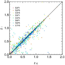
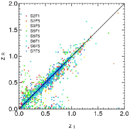
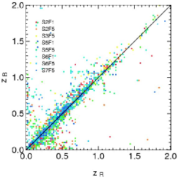
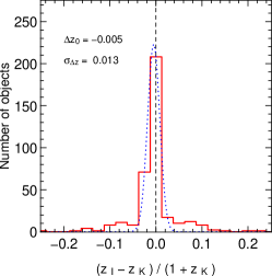
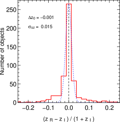
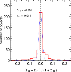
Figure 19: Left-hand panels: Comparison of photometric redshifts from the $I$-selected MUNICS catalogue to those from the $K$-selected MUNICS sample. Middle panels: The same for the $R$ and the $I$-selected catalogue. Right-hand panels: The same for the $B$ and the $R$-selected catalogue. The lower panels show histograms of the redshift differences together with a Gaussian fit showing the quality of the photometric redshifts.

Appendix A Photometric Redshifts in Different Samples

It is an important consistency check to compare the photometric redshifts of an object present in two different selection catalogues. Note that the two redshifts do not have to be the same in the case of MUNICS, since small differences in object centring and differences in the object’s shape in the different detection images lead to slightly different photometry. Direct comparison of magnitudes in the same filter, but derived in the different selection catalogues show excellent agreement (comparison plots are published in Feulner, 2004).

Due to this small differences in the objects’ photometry, the result for a comparison of the photometric redshifts in different catalogues is a scatter around the one-to-one relation, as shown in Figure 19. However, the general agreement is extremely good, as can be seen from the histograms of redshift differences also shown in the Figure. The deviation from a zero redshift difference is smaller than 0.01 in $z$, and the $\sigma$ of the best-fitting Gaussian is smaller than 0.02, which is the redshift binning size of our photometric redshift algorithm.

References

- Alcalá et al. (2004) Alcalá J. M., et al., 2004, A&A, 428, 339
- Arnouts et al. (1999) Arnouts S., D’Odorico S., Cristiani S., Zaggia S., Fontana A., Giallongo E., 1999, A&A, 341, 641
- Arnouts et al. (2001) Arnouts S., Vandame B., Benoist C., Groenewegen M. A. T., da Costa L., Schirmer M., Mignani R. P., Slijkhuis R., Hatziminaoglou E., Hook R., Madejsky R., Rité C., Wicenec A., 2001, A&A, 379, 740
- Bauer et al. (2005) Bauer A. E., Drory N., Hill G. J., Feulner G., 2005, ApJ, 621, L89
- Bell et al. (2005) Bell E. F., Papovich C., Wolf C., Le Floc’h E., Caldwell J. A. R., Barden M., Egami E., McIntosh D. H., Meisenheimer K., Pérez-González P. G., Rieke G. H., Rieke M. J., Rigby J. R., Rix H., 2005, ApJ, 625, 23
- Bender et al. (2001) Bender R., et al., 2001, in Cristiani S., Renzini A., Williams R. E., eds, Deep Fields The FORS Deep Field: Photometric Data and Photometric Redshifts. Springer, p. 96
- Benítez (2000) Benítez N., 2000, ApJ, 536, 571
- Bershady et al. (1998) Bershady M. A., Lowenthal J. D., Koo D. C., 1998, ApJ, 505, 50
- Bertin & Dennefeld (1997) Bertin E., Dennefeld M., 1997, A&A, 317, 43
- Blanton et al. (2003) Blanton M. R., et al., 2003, ApJ, 592, 819
- Botzler et al. (2007) Botzler C., Snigula J., Bender R., Feulner G., Goranova Y., Hopp U., 2007, MNRAS, submitted (MUNICS VIII)
- Botzler (2004) Botzler C. S., 2004, PhD thesis, Ludwig–Maximilians–Universität München
- Botzler et al. (2004) Botzler C. S., Snigula J., Bender R., Hopp U., 2004, MNRAS, 349, 425
- Brinchmann et al. (2004) Brinchmann J., Charlot S., White S. D. M., Tremonti C., Kauffmann G., Heckman T., Brinkmann J., 2004, MNRAS, 351, 1151
- Bruzual & Charlot (2003) Bruzual G., Charlot S., 2003, MNRAS, 344, 1000
- Capak et al. (2004) Capak P., Cowie L. L., Hu E. M., Barger A. J., Dickinson M., Fernandez E., Giavalisco M., Komiyama Y., Kretchmer C., McNally C., Miyazaki S., Okamura S., Stern D., 2004, AJ, 127, 180
- Casertano et al. (1995) Casertano S., Ratnatunga K. U., Griffiths R. E., Im M., Neuschaefer L. W., Ostrander E. J., Windhorst R. A., 1995, ApJ, 453, 599
- Cimatti et al. (2002) Cimatti A., Mignoli M., Daddi E., Pozzetti L., Fontana A., Saracco P., Poli F., Renzini A., Zamorani G., Broadhurst T., Cristiani S., D’Odorico S., Giallongo E., Gilmozzi R., Menci N., 2002, A&A, 392, 395
- Cole et al. (2001) Cole S., et al., 2001, MNRAS, 326, 255
- Colless (1997) Colless M., 1997, in ASSL Vol. 212: Wide-field spectroscopy Wide Field Spectroscopy and the Universe. p. 227
- Couch et al. (1993) Couch W. J., Jurcevic J. S., Boyle B. J., 1993, MNRAS, 260, 241
- Couch & Newell (1984) Couch W. J., Newell E. B., 1984, ApJS, 56, 143
- Cowie et al. (1994) Cowie L. L., Gardner J. P., Hu E. M., Songaila A., Hodapp K.-W., Wainscoat R. J., 1994, ApJ, 434, 114
- Cristóbal-Hornillos et al. (2003) Cristóbal-Hornillos D., Balcells M., Prieto M., Guzmán R., Gallego J., Cardiel N., Serrano Á., Pelló R., 2003, ApJ, 595, 71
- Djorgovski et al. (1995) Djorgovski S., Soifer B. T., Pahre M. A., Larkin J. E., Smith J. D., Neugebauer G., Smail I., Matthews K., Hogg D. W., Blandford R. D., Cohen J., Harrison W., Nelson J., 1995, ApJ, 438, L13
- Driver et al. (2005) Driver S. P., Liske J., Cross N. J. G., De Propris R., Allen P. D., 2005, MNRAS, 360, 81
- Driver et al. (1994) Driver S. P., Phillipps S., Davies J. I., Morgan I., Disney M. J., 1994, MNRAS, 266, 155
- Driver et al. (1995) Driver S. P., Windhorst R. A., Ostrander E. J., Keel W. C., Griffiths R. E., Ratnatunga K. U., 1995, ApJ, 449, L23
- Drory (2003) Drory N., 2003, A&A, 397, 371
- Drory et al. (2003) Drory N., Bender R., Feulner G., Hopp U., Maraston C., Snigula J., Hill G. J., 2003, ApJ, 595, 698 (MUNICS II)
- Drory et al. (2004) Drory N., Bender R., Feulner G., Hopp U., Maraston C., Snigula J., Hill G. J., 2004, ApJ, 608, 742 (MUNICS VI)
- Drory et al. (2004) Drory N., Bender R., Hopp U., 2004, ApJ, 616, L103
- Drory et al. (2001) Drory N., Bender R., Snigula J., Feulner G., Hopp U., Maraston C., Hill G. J., Mendes de Oliveira C., 2001, ApJ, 562, L111 (MUNICS III)
- Drory et al. (2001) Drory N., Feulner G., Bender R., Botzler C. S., Hopp U., Maraston C., Mendes de Oliveira C., Snigula J., 2001, MNRAS, 325, 550 (MUNICS I)
- Ebeling (2003) Ebeling H., 2003, MNRAS, 340, 1269
- Ebeling (2004) Ebeling H., 2004, MNRAS, 349, 768
- Ellis (1997) Ellis R. S., 1997, ARA&A, 35, 389
- Ellis et al. (1996) Ellis R. S., Colless M., Broadhurst T., Heyl J., Glazebrook K., 1996, MNRAS, 280, 235
- Feulner (2004) Feulner G., 2004, PhD thesis, Ludwig-Maximilians-Universität München
- Feulner et al. (2003) Feulner G., Bender R., Drory N., Hopp U., Snigula J., Hill G. J., 2003, MNRAS, 342, 605 (MUNICS V)
- Feulner et al. (2005) Feulner G., Gabasch A., Salvato M., Drory N., Hopp U., Bender R., 2005, ApJ, 633, L9
- Feulner et al. (2005) Feulner G., Goranova Y., Drory N., Hopp U., Bender R., 2005, MNRAS, 358, L1 (MUNICS VII)
- Feulner et al. (2006) Feulner G., Hopp U., Botzler C. S., 2006, A&A, 451, L13
- Gabasch et al. (2004) Gabasch A., Bender R., Seitz S., Hopp U., Saglia R. P., Feulner G., Snigula J., Drory N., Appenzeller I., Heidt J., Mehlert D., Noll S., Böhm A., Jäger K., Ziegler B., Fricke K. J., 2004, A&A, 421, 41
- Gabasch et al. (2006) Gabasch A., Hopp U., Feulner G., Bender R., Seitz S., Saglia R. P., Snigula J., Drory N., Appenzeller I., Heidt J., Mehlert D., Noll S., Böhm A., Jäger K., Ziegler B., 2006, A&A, 448, 101
- Gardner et al. (1993) Gardner J. P., Cowie L. L., Wainscoat R. J., 1993, ApJ, 415, L9
- Gardner et al. (1996) Gardner J. P., Sharples R. M., Carrasco B. E., Frenk C. S., 1996, MNRAS, 282, L1
- Gehrels (1986) Gehrels N., 1986, ApJ, 303, 336
- Gerke et al. (2007) Gerke B., et al., 2007, MNRAS, submitted, astro-ph/0608569
- Glazebrook et al. (1995) Glazebrook K., Peacock J. A., Miller L., Collins C. A., 1995, MNRAS, 275, 169
- Hall & Mackay (1984) Hall P., Mackay C. D., 1984, MNRAS, 210, 979
- Heidt et al. (2003) Heidt J., et al., 2003, A&A, 398, 49
- Heydon-Dumbleton et al. (1989) Heydon-Dumbleton N. H., Collins C. A., MacGillivray H. T., 1989, MNRAS, 238, 379
- Heyl et al. (1997) Heyl J., Colless M., Ellis R. S., Broadhurst T., 1997, MNRAS, 285, 613
- Hogg et al. (1997) Hogg D. W., Pahre M. A., McCarthy J. K., Cohen J. G., Blandford R., Smail I., Soifer B. T., 1997, MNRAS, 288, 404
- Huang et al. (1998) Huang J., Cowie L. L., Luppino G. A., 1998, ApJ, 496, 31
- Huang et al. (1997) Huang J. S., Cowie L. L., Gardner J. P., Hu E. M., Songaila A., Wainscoat R. J., 1997, ApJ, 476, 12
- Huang et al. (2001) Huang J.-S., Thompson D., Kümmel M. W., Meisenheimer K., Wolf C., Beckwith S. V. W., Fockenbrock R., Fried J. W., Hippelein H., von Kuhlmann B., Phleps S., Röser H.-J., Thommes E., 2001, A&A, 368, 787
- Infante et al. (1986) Infante L., Pritchet C., Quintana H., 1986, AJ, 91, 217
- Jahnke & Wisotzki (2003) Jahnke K., Wisotzki L., 2003, MNRAS, 346, 304
- Jarvis & Tyson (1981) Jarvis J. F., Tyson J. A., 1981, AJ, 86, 476
- Jones et al. (2006) Jones D. H., Peterson B. A., Colless M., Saunders W., 2006, MNRAS, 369, 25
- Jones et al. (1991) Jones L. R., Fong R., Shanks T., Ellis R. S., Peterson B. A., 1991, MNRAS, 249, 481
- Juneau et al. (2005) Juneau S., Glazebrook K., Crampton D., McCarthy P. J., Savaglio S., Abraham R., Carlberg R. G., Chen H., Le Borgne D., Marzke R. O., Roth K., Jørgensen I., Hook I., Murowinski R., 2005, ApJ, 619, L135
- Kümmel & Wagner (2001) Kümmel M. W., Wagner S. J., 2001, A&A, 370, 384
- Kashikawa et al. (2004) Kashikawa N., et al., 2004, PASJ, 56, 1011
- Kauffmann et al. (2004) Kauffmann G., White S., Heckman T., Ménard B., Brinchmann J., Charlot S., Tremonti C., Brinkmann J., 2004, MNRAS, 353, 713
- Koo (1986) Koo D. C., 1986, ApJ, 311, 651
- Kron (1978) Kron R. G., 1978, PhD thesis, California University, Berkeley
- Lilly et al. (1991) Lilly S. J., Cowie L. L., Gardner J. P., 1991, ApJ, 369, 79
- Lilly et al. (1996) Lilly S. J., Le Fèvre O., Hammer F., Crampton D., 1996, ApJ, 460, L1
- Lilly et al. (1995) Lilly S. J., Tresse L., Hammer F., Crampton D., Le Fèvre O., 1995, ApJ, 455, 108
- Madau et al. (1998) Madau P., Pozzetti L., Dickinson M., 1998, ApJ, 498, 106
- Maddox et al. (1990) Maddox S. J., Efstathiou G., Sutherland W. J., Loveday J., 1990, MNRAS, 243, 692
- Maddox et al. (1990) Maddox S. J., Sutherland W. J., Efstathiou G., Loveday J., Peterson B. A., 1990, MNRAS, 247, 1
- Maihara et al. (2001) Maihara T., et al., 2001, PASJ, 53, 25
- Martini (2001) Martini P., 2001, AJ, 121, 2301
- McCracken et al. (2000) McCracken H. J., Metcalfe N., Shanks T., Campos A., Gardner J. P., Fong R., 2000, MNRAS, 311, 707
- McLeod et al. (1995) McLeod B. A., Bernstein G. M., Rieke M. J., Tollestrup E. V., Fazio G. G., 1995, ApJS, 96, 117
- Metcalfe et al. (1995) Metcalfe N., Fong R., Shanks T., 1995, MNRAS, 274, 769
- Metcalfe et al. (1998) Metcalfe N., Ratcliffe A., Shanks T., Fong R., 1998, MNRAS, 294, 147
- Metcalfe et al. (1996) Metcalfe N., Shanks T., Campos A., Fong R., Gardner J. P., 1996, Nat, 383, 236
- Metcalfe et al. (2001) Metcalfe N., Shanks T., Campos A., McCracken H. J., Fong R., 2001, MNRAS, 323, 795
- Metcalfe et al. (1991) Metcalfe N., Shanks T., Fong R., Jones L. R., 1991, MNRAS, 249, 498
- Metcalfe et al. (1995) Metcalfe N., Shanks T., Fong R., Roche N., 1995, MNRAS, 273, 257
- Minowa et al. (2005) Minowa Y., Kobayashi N., Yoshii Y., Totani T., Maihara T., Iwamuro F., Takami H., Takato N., Hayano Y., Terada H., Oya S., Iye M., Tokunaga A. T., 2005, ApJ, 629, 29
- Moustakas et al. (1997) Moustakas L. A., Davis M., Graham J. R., Silk J., Peterson B. A., Yoshii Y., 1997, ApJ, 475, 445
- Peterson et al. (1986) Peterson B. A., Ellis R. S., Efstathiou G., Shanks T., Bean A. J., Fong R., Zen-Long Z., 1986, MNRAS, 221, 233
- Picard (1991) Picard A., 1991, AJ, 102, 445
- Postman et al. (1998) Postman M., Lauer T. R., Szapudi I., Oegerle W., 1998, ApJ, 506, 33
- Rix & Rieke (1993) Rix H., Rieke M. J., 1993, ApJ, 418, 123
- Saha (1995) Saha P., 1995, AJ, 110, 916
- Salpeter (1955) Salpeter E. E., 1955, ApJ, 121, 161
- Saracco et al. (1999) Saracco P., D’Odorico S., Moorwood A., Buzzoni A., Cuby J. ., Lidman C., 1999, A&A, 349, 751
- Saracco et al. (2001) Saracco P., Giallongo E., Cristiani S., D’Odorico S., Fontana A., Iovino A., Poli F., Vanzella E., 2001, A&A, 375, 1
- Saracco et al. (1997) Saracco P., Iovino A., Garilli B., Maccagni D., Chincarini G., 1997, AJ, 114, 887
- Schechter (1976) Schechter P., 1976, ApJ, 203, 297
- Schmidt (1968) Schmidt M., 1968, ApJ, 151, 393
- Smail et al. (1995) Smail I., Hogg D. W., Yan L., Cohen J. G., 1995, ApJ, 449, L105
- Snigula et al. (2002) Snigula J., Drory N., Bender R., Botzler C. S., Feulner G., Hopp U., 2002, MNRAS, 336, 1329 (MUNICS IV)
- Soifer et al. (1994) Soifer B. T., Matthews K., Djorgovski S., Larkin J., Graham J. R., Harrison W., Jernigan G., Lin S., Nelson J., Neugebauer G., Smith G., Smith J. D., Ziomkowski C., 1994, ApJ, 420, L1
- Steidel & Hamilton (1993) Steidel C. C., Hamilton D., 1993, AJ, 105, 2017
- Stevenson et al. (1986) Stevenson P. R. F., Shanks T., Fong R., 1986, in Spectral Evolution of Galaxies New observations of galaxy number counts. pp 439–445
- Szokoly et al. (1998) Szokoly G. P., Subbarao M. U., Connolly A. J., Mobasher B., 1998, ApJ, 492, 452
- Teplitz et al. (1999) Teplitz H. I., McLean I. S., Malkan M. A., 1999, ApJ, 520, 469
- Tyson (1988) Tyson J. A., 1988, AJ, 96, 1
- Väisänen et al. (2000) Väisänen P., Tollestrup E. V., Willner S. P., Cohen M., 2000, ApJ, 540, 593
- Weinmann et al. (2006) Weinmann S. M., van den Bosch F. C., Yang X., Mo H. J., 2006, MNRAS, 366, 2
- Williams et al. (1996) Williams R. E., Blacker B., Dickinson M., Dixon W. V. D., Ferguson H. C., Fruchter A. S., Giavalisco M., Gilliland R. L., Heyer I., Katsanis R., Levay Z., Lucas R. A., McElroy D. B., Petro L., Postman M., Adorf H., Hook R., 1996, AJ, 112, 1335
- Yasuda et al. (2001) Yasuda N., et al., 2001, AJ, 122, 1104
- Yee & Green (1987) Yee H. K. C., Green R. F., 1987, ApJ, 319, 28