Observational Constraints on Dark Energy and Cosmic Curvature

Abstract

Current observational bounds on dark energy depend on our assumptions about the curvature of the universe. We present a simple and efficient method for incorporating constraints from Cosmic Microwave Background (CMB) anisotropy data, and use it to derive constraints on cosmic curvature and dark energy density as a free function of cosmic time using current CMB, Type Ia supernova (SN Ia), and baryon acoustic oscillation (BAO) data.

We show that there are two CMB shift parameters, $R\equiv\sqrt{\Omega_{m}H_{0}^{2}}\,r(z_{CMB})$ (the scaled distance to recombination) and $l_{a}\equiv\pi r(z_{CMB})/r_{s}(z_{CMB})$ (the angular scale of the sound horizon at recombination), with measured values that are nearly uncorrelated with each other. Allowing nonzero cosmic curvature, the three-year WMAP data give $R=1.71\pm 0.03$, $l_{a}=302.5\pm 1.2$, and $\Omega_{b}h^{2}=0.02173\pm 0.00082$, independent of the dark energy model. The corresponding bounds for a flat universe are $R=1.70\pm 0.03$, $l_{a}=302.2\pm 1.2$, and $\Omega_{b}h^{2}=0.022\pm 0.00082$. We give the covariance matrix of ($R$, $l_{a}$, $\Omega_{b}h^{2}$) from the three-year WMAP data. We find that ($R$, $l_{a}$, $\Omega_{b}h^{2}$) provide an efficient and intuitive summary of CMB data as far as dark energy constraints are concerned.

Assuming the HST prior of $H_{0}=72\pm 8\,$(km/s)Mpc^-1, using 182 SNe Ia (from the HST/GOODS program, the first year Supernova Legacy Survey, and nearby SN Ia surveys), ($R$, $l_{a}$, $\Omega_{b}h^{2}$) from WMAP three year data, and SDSS measurement of the baryon acoustic oscillation scale, we find that dark energy density is consistent with a constant in cosmic time, with marginal deviations from a cosmological constant that may reflect current systematic uncertainties or true evolution in dark energy. A flat universe is allowed by current data: $\Omega_{k}=-0.006_{-0.012}^{+0.013}$${}_{-0.025}^{+0.025}$ for assuming that the dark energy equation of state $w_{X}(z)$ is constant, and $\Omega_{k}=-0.002_{-0.018}^{+0.018}$${}_{-0.032}^{+0.041}$ for $w_{X}(z)=w_{0}+w_{a}(1-a)$ (68% and 95% confidence levels). The bounds on cosmic curvature are less stringent if dark energy density is allowed to be a free function of cosmic time, and are also dependent on the assumption about the early time property of dark energy. We demonstrate this by studying two examples. Significant improvement in dark energy and cosmic curvature constraints is expected as a result of future dark energy and CMB experiments.

I Introduction

The unknown cause for the observed cosmic acceleration Riess et al. (1998); Perlmutter et al. (1999), dubbed “dark energy”, remains the most compelling mystery in cosmology today. Dark energy could be an unknown energy component Freese et al. (1987); Linde (1987); Peebles & Ratra (1988); Wetterich (1988); Frieman et al. (1995); Caldwell, Dave & Steinhardt (1998), or a modification of general relativity (Sahni & Habib, 1998; Parker & Raval, 1999; Boisseau et al., 2000; Dvali, Gabadadze, & Porrati, 2000; Mersini, Bastero-Gil, & Kanti, 2001; Freese & Lewis, 2002). Padmanabhan (2003) and Peebles & Ratra (2003) contain reviews of many models. Dark energy model-building is a very active research area. For recent dark energy models, see for example, Carroll et al. (2004); Onemli & Woodard (2004); Cardone et al. (2005); Kolb, Matarrese, & Riotto (2005); Caldwell (2006); Kahya & Onemli (2006); DeFelice (2007); Koi (2007); Ng (2007). Current observational data continue to be consistent with dark energy being a cosmological constant, but the evidence for a cosmological constant is not conclusive and more exotic possibilities are still allowed (see, for example, Wang & Tegmark (2004, 2005); Alam & Sahni (2005); Daly & Djorgovski (2005); Jassal, Bagla, & Padmanabhan (2005a, b); Barger (2006); Dick, Knox, & Chu (2006); Huterer (2006); Jassal, Bagla, & Padmanabhan (2006); Liddle (2006); Nesseris & Perivolaropoulos (2006); Schimd et al. (2006); Sumu (2006); Wilson, Chen, & Ratra (2006); Xia (2006); Alam (2007); Davis (2007); Wei (2007); Zhang (2007); Zun (2007)).

While the universe is completely consistent with being flat under a $\Lambda$CDM hypothesis, it is important to note that the observational bounds on dark energy and the curvature of the universe are closely related. Cosmic Microwave Background (CMB) anisotropy data provide the most stringent constraints on cosmic curvature $\Omega_{k}$. Assuming that dark energy is a cosmological constant, the three-year WMAP data give $\Omega_{k}=-0.15\pm 0.11$, and this improves dramatically to $\Omega_{k}=-0.005\pm 0.006$ with the addition of galaxy survey data from the SDSS sdss (2004) (2dF data 2df (2006) also give a similar improvement) Spergel et al. (2006). The effect of allowing non-zero curvature on constraining some dark energy models has been studied by Polarski & Ranquet (2005); Franca (2006); Ichikawa & Takahashi (2006); Ichikawa et al. (2006); Clarkson (2007); Gong (2007); Ichikawa (2007); Zhao (2007); Wright (2007).

In this paper, we present a simple and efficient method for incorporating constraints from the CMB data into an analysis with other cosmological data in constraining dark energy without assuming a flat universe. Uisng this method, we derive constraints on dark energy and cosmic curvature using CMB, type Ia supernova (SN Ia) and galaxy survey data.

We describe our method in Sec.II, present our results in Sec.III, and conclude in Sec.IV.

II Method

The comoving distance from the observer to redshift $z$ is given by

$$r(z)=cH_{0}^{-1}\,|\Omega_{k}|^{-1/2}{\rm sinn}[|\Omega_{k}|^{1/2}\,\Gamma(z)],$$ (1)

$$\Gamma(z)=\int_{0}^{z}\frac{dz^{\prime}}{E(z^{\prime})},\hskip 28.45274ptE(z)=H(z)/H_{0}$$

where $\Omega_{k}=-k/H_{0}^{2}$ with $k$ denoting the curvature constant, and ${\rm sinn}(x)=\sin(x)$, $x$, $\sinh(x)$ for $\Omega_{k}<0$, $\Omega_{k}=0$, and $\Omega_{k}>0$ respectively, and

$$E(z)=\left[\Omega_{m}(1+z)^{3}+\Omega_{\rm rad}(1+z)^{4}+\Omega_{k}(1+z)^{2}+\Omega_{X}X(z)\right]^{1/2}$$ (2)

with $\Omega_{X}=1-\Omega_{m}-\Omega_{\rm rad}-\Omega_{k}$, and the dark energy density function $X(z)\equiv\rho_{X}(z)/\rho_{X}(0)$.

CMB data give us the comoving distance to the recombination surface $r(z_{CMB})$ with $z_{CMB}=1089$, and the comoving sound horizon at recombinationEisenstein & Hu (1998); Page (2003)

$$r_{s}(z_{CMB}) = \int_{0}^{t_{CMB}}\frac{c_{s}\,dt}{a}=cH_{0}^{-1}\int_{z_{CMB}}^{\infty}dz\,\frac{c_{s}}{E(z)},$$ (3)

$$= cH_{0}^{-1}\int_{0}^{a_{CMB}}\frac{da}{\sqrt{3(1+\overline{R_{b}}\,a)\,a^{4}E^{2}(z)}},$$

where $a$ is the cosmic scale factor, $a_{CMB}=1/(1+z_{CMB})$, and $a^{4}E^{2}(z)=\Omega_{m}(a+a_{\rm eq})+\Omega_{k}a^{2}+\Omega_{X}X(z)a^{4}$, with $a_{\rm eq}=\Omega_{\rm rad}/\Omega_{m}=1/(1+z_{\rm eq})$, and $z_{\rm eq}=2.5\times 10^{4}\Omega_{m}h^{2}(T_{CMB}/2.7\,{\rm K})^{-4}$. The sound speed is $c_{s}=1/\sqrt{3(1+\overline{R_{b}}\,a)}$, with $\overline{R_{b}}\,a=3\rho_{b}/(4\rho_{\gamma})$, $\overline{R_{b}}=31500\Omega_{b}h^{2}(T_{CMB}/2.7\,{\rm K})^{-4}$. COBE four year data give $T_{CMB}=2.728\,$K Fixsen (1996). The angular scale of the sound horizon at recombination is defined as $l_{a}=\pi r(z_{CMB})/r_{s}(z_{CMB})$ Page (2003).

Note that it is important to use the full expression given in Eq.(3) in making predictions for $l_{a}$ for dynamical dark energy models. Fig.1 shows how the dark energy density $X(z)\equiv\rho_{X}(z)/\rho_{X}(0)$ compares with the matter density $\rho_{m}(z)/\rho_{m}(0)=(1+z)^{3}$ for a two parameter dark energy model with dark energy equation of state $w_{X}(z)=w_{0}+w_{a}(1-a)$ Chev01 (2001) which corresponds to $X(z)=a^{-3(1+w_{0}+w_{a})}e^{3w_{a}(a-1)}$. For models with $w_{0}+w_{a}>0$, the dark energy contribution to the expansion rate of the universe dominates over that of matter at high $z$. For models that allow significant early dark energy (as in the $w_{X}(z)=w_{0}+w_{a}(1-a)$ model), $l_{a}$ can be underestimated by $20-40$% if the dark energy contribution to $r_{s}(z_{CMB})$ is ignored.

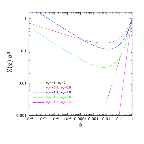
Figure 1: Ratio of the dark energy density $X(z)\equiv\rho_{X}(z)/\rho_{X}(0)$ and the matter density $\rho_{m}(z)/\rho_{m}(0)=(1+z)^{3}$ for dark energy models with dark energy equation of state $w_{X}(z)=w_{0}+w_{a}(1-a)$.

We will show that the CMB shift parameters

$$R\equiv\sqrt{\Omega_{m}H_{0}^{2}}\,r(z_{CMB}),\hskip 7.22743ptl_{a}\equiv\pi r(z_{CMB})/r_{s}(z_{CMB}),$$ (4)

together with $\Omega_{b}h^{2}$, provide an efficient summary of CMB data as far as dark energy constraints go (see Sec.IIIA).

SN Ia data give the luminosity distance as a function of redshift, $d_{L}(z)=(1+z)\,r(z)$. We use 182 SNe Ia from the HST/GOODS program Riess (2007) and the first year SNLS Astier et al. (2005), together with nearby SN Ia data, as compiled by Riess (2007). We do not include the ESSENCE data Wood (2007), as these are not yet derived using the same method as thosed used in Riess (2007). Combining SN Ia data derived using different analysis techniques leads to systematic effects in the estimated SN distance moduli Wang (2000); Wood (2007). Appendix A describes in detail how we use SN Ia data (flux-averaged and marginalized over $H_{0}$) in this paper.

We also use the SDSS baryon acoustic oscillation (BAO) scale measurement by adding the following term to the $\chi^{2}$ of a model:

$$\chi^{2}_{BAO}=\left[\frac{(A-A_{BAO})}{\sigma_{A}}\right]^{2},$$ (5)

where $A$ is defined as

$$A=\left[r^{2}(z_{BAO})\,\frac{cz_{BAO}}{H(z_{BAO})}\right]^{1/3}\,\frac{\left(\Omega_{m}H_{0}^{2}\right)^{1/2}}{cz_{BAO}},$$ (6)

and $A_{BAO}=0.469\,(n_{S}/0.98)^{-0.35}$, $\sigma_{A}=0.017$, and $z_{BAO}=0.35$ (independent of a dark energy model) Eisenstein et al. (2005). We take the scalar spectral index $n_{S}=0.95$ as measured by WMAP3 (Spergel et al., 2006).

For Gaussian distributed measurements, the likelihood function $L\propto e^{-\chi^{2}/2}$, with

$$\chi^{2}=\chi^{2}_{CMB}+\chi^{2}_{SNe}+\chi^{2}_{BAO},$$ (7)

where $\chi^{2}_{CMB}$ is given in Eq.(10) in Sec.IIIA, $\chi^{2}_{SNe}$ is given in Eq.(13) in Appendix A, and $\chi^{2}_{BAO}$ is given in Eq.(5).

We derive constraints on the dark energy density function $X(z)\equiv\rho_{X}(z)/\rho_{X}(0)$ as a free function at $z\leq z_{cut}$, with its value at redshifts $z_{i}=z_{cut}(i/n)$ (i=1, 2, …, $n$), $X(z_{i})$, treated as $n$ independent parameters estimated from data. We use $n=3$ and $z_{\rm cut}=1.4$ in this paper. We use cubic spline interpolation to obtain values of $X(z)$ at other values of $z$ at $z<z_{cut}$ (Wang & Tegmark, 2004). The number of currently published SNe Ia is very few beyond $z_{\rm cut}=1.4$. For $z>z_{\rm cut}$, we assume $X(z)$ to be matched on to either a powerlaw Wang & Tegmark (2004):

$$X(z)=X(z_{\rm cut})\left(\frac{1+z}{1+z_{\rm cut}}\right)^{\alpha},$$ (8)

or an exponential function:

$$X(z)=X(z_{\rm cut})\,e^{\alpha(z-zcut)}.$$ (9)

We impose a prior of $\alpha\geq-3$ as $\alpha$ is not bounded from below. Our approach effectively decouples late time dark energy (which is responsible for the observed recent cosmic acceleration and is probed directly by SN Ia data) and early time dark energy (which is poorly constrained) by parametrizing the latter with an additional parameter estimated from data.

For comparison with the results of others, we also derive constraints for models with dark energy equation of state $w_{X}(z)=w_{0}+w_{a}(1-a)$. This parametrization has the advantage of not requiring a cutoff to obtain a finite dark energy equation of state at high $z$ (which is not true for the $w_{X}(z)=w_{0}+w^{\prime}z$ parametrization), but it does allow significant early dark energy (which can cause problems for Big Bang Nucleosynthesis Steigman (2006) and cosmic structure formation Sandvik (2004)), unless a cutoff is imposed. This dilemma illustrates the limited usefulness of simple parametrizations of dark energy.

For all the dark energy constraints from combining the different data sets presented in this paper, we marginalize the SN Ia data over $H_{0}$ in flux-averaging statistics (described in the next subsection), and impose a prior of $H_{0}=72\pm 8\,$(km/s)Mpc^-1 from the HST Cepheid variable star observations HST_H0 (2001).

We run a Monte Carlo Markov Chain (MCMC) based on the MCMC engine of Lewis02 (2002) to obtain ${\cal O}$($10^{6}$) samples for each set of results presented in this paper. For the full CMB analysis we used the WMAP three year temperature and polarization power spectra Spergel et al. (2006) with version 2 of their likelihood code WMAP (2006) together with theoretical power spectra generated by CAMB (with perturbations in dark energy) Lewis, Challinor, & Lasenby (2000); the parameters used are ($\Omega_{k}$, $\Omega_{b}h^{2}$, $\Omega_{m}h^{2}$, $h$, $A_{s}$, $\tau$, $n_{s}$, $\mbox{\bf p}_{DE}$). For the combined data analysis using CMB shift parameters, the parameters used are ($\Omega_{k}$, $\Omega_{m}$, $h$, $\Omega_{b}h^{2}$, $\mbox{\bf p}_{DE}$). The dark energy parameter set $\mbox{\bf p}_{DE}=w$ for a constant $w_{X}(z)$, $\mbox{\bf p}_{DE}=(w_{0},w_{a})$ for $w_{X}(z)=w_{0}+w_{a}(1-a)$, and $\mbox{\bf p}_{DE}=(X(z_{1}),X(z_{2}),X(z_{3}),\alpha)$ for the general case. We assumed flat priors for all the parameters, and allowed ranges of the parameters wide enough such that further increasing the allowed ranges has no impact on the results (with the exception of constraining $w$ and $(w_{0},w_{a})$ using CMB data only where we have to impose fixed allowed ranges for $w$ and $(w_{0},w_{a})$ since these are not well constrained). The chains typically have worst e-values (the variance(mean)/mean(variance) of 1/2 chains) much smaller than 0.01, indicating convergence. The chains are subsequently appropriately thinned to ensure independent samples.

III Results

III.1 A Simple and Efficient Method for Incorporating CMB data

III.1.1 A roadmap of our method

We propose a simple and efficient method for dark energy data analysis, with $\chi^{2}=-2\,\ln L=\chi^{2}_{CMB}+\chi^{2}_{SNe}+\chi^{2}_{BAO}$, where $\chi^{2}_{CMB}$ is given by constraints on $(R,l_{a},\Omega_{b}h^{2})$ (see Eq.[10] in Sec.IIIA), $\chi^{2}_{SNe}$ is given by SN Ia data flux-averaged and marginalized over $H_{0}$ (see Eq.[13] in Appendix A), and $\chi^{2}_{BAO}$ is given by Eisenstein et al. (2005) (see Eq.[5]). In our method, CMB data are incorporated by using constraints on $(R,l_{a},\Omega_{b}h^{2})$, instead of using the full CMB power spectra. In Sec.III.1.2 below, we will show that $(R,l_{a},\Omega_{b}h^{2})$ provide an efficient and intuitive summary of CMB data as far as dark energy constraints are concerned.

III.1.2 Justification of our method

We have performed MCMC calculations using only the full CMB temperature and polarization angular power spectra from WMAP three year observations, without assuming spatial flatness, and without imposing any priors on $H_{0}$. These calculations are quite time consuming. We have used these to derived the results in Fig.2 and Tables I-II.

Fig.2 shows that allowing nonzero cosmic curvature, the three-year WMAP data give measurements of ($R$, $l_{a}$, $\Omega_{b}h^{2}$) that are independent of the dark energy model. The measurements of ($R$, $l_{a}$, $\Omega_{b}h^{2}$) differ slightly in a flat universe because of the correlation of curvature with other cosmological parameters when spatial flatness is not assumed. Table I gives the parameters for the Gaussian fits to the probability distribution functions of $(R,l_{a},\Omega_{b}h^{2},\Omega_{m}h^{2},r_{s}(z_{CMB}),r(z_{CMB}))$ from the three-year WMAP data. These fits are independent of the dark energy model assumed. The constraints on ($\Omega_{m}h^{2}$, $r_{s}(z_{CMB})$, $r(z_{CMB})$) are also independent of the assumption about cosmic curvature.

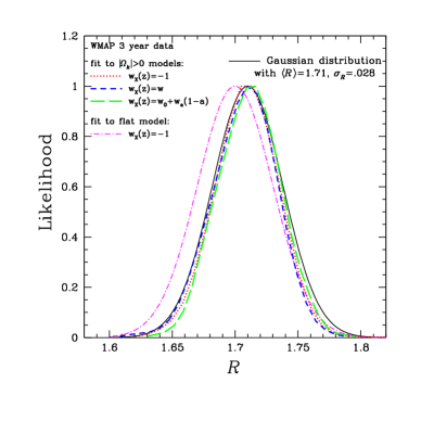
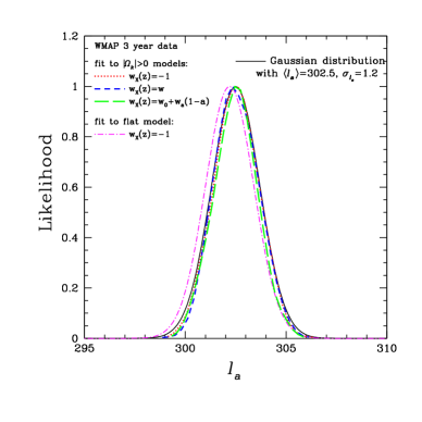
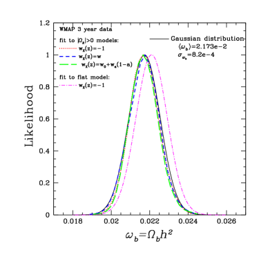
Figure 2: The scaled distance to recombination $R$, the angular scale of the sound horizon at recombination $l_{a}$, and the baryon density $\Omega_{b}h^{2}$ from the three-year WMAP data.

Table II gives the normalized covariance matrices for $(R,l_{a},\Omega_{b}h^{2},\Omega_{m}h^{2},r_{s}(z_{CMB}),r(z_{CMB}))$ from the three-year WMAP data for a $\Lambda$CDM model for models with and without curvature. These are appropriate to use with Table I; models with non-constant dark energy density give slightly smaller correlations between the parameters. Note that we have included ($\Omega_{m}h^{2},r_{s}(z_{CMB}),r(z_{CMB}))$ in Tables I-II to show that although these three parameters are well constrained by CMB data, they are strongly correlated with each other, in contrast to the parameters we have chosen, $(R,l_{a},\Omega_{b}h^{2})$.

Table 1: The parameters for the Gaussian fits to the probability distribution functions of $(R,l_{a},\Omega_{b}h^{2},\Omega_{m}h^{2},r_{s}(z_{CMB}),r(z_{CMB}))$ from the three-year WMAP data, independent of the dark energy model assumed.

Parameter	mean	rms variance
$\Omega_{m}h^{2}$	0.1284	0.0086
$r_{s}(z_{CMB})$/Mpc	148.55	2.60
$r(z_{CMB})$/Mpc	14305	285
	$\Omega_{k}\neq 0$
$R$	1.71	0.03
$l_{a}$	302.5	1.2
$\Omega_{b}h^{2}$	0.02173	0.00082
	$\Omega_{k}=0$
$R$	1.70	0.03
$l_{a}$	302.2	1.2
$\Omega_{b}h^{2}$	0.022	0.00082

Table 2: Normalized covariance matrices for $(R,l_{a},\Omega_{b}h^{2},\Omega_{m}h^{2},r_{s}(z_{CMB}),r(z_{CMB}))$ fromthe WMAP three year data.

	$R$	$l_{a}$	$\Omega_{b}h^{2}$	$\Omega_{m}h^{2}$	$r_{s}(z_{CMB})$	$r(z_{CMB})$
			$\Omega_{k}\neq 0$
$R$	0.1000E+01	$-$0.1237E+00	0.6627E$-$01	0.9332E+00	$-$0.8805E+00	$-$0.8023E+00
$l_{a}$	$-$0.1237E+00	0.1000E+01	$-$0.6722E+00	$-$0.4458E+00	0.5214E+00	0.6569E+00
$\Omega_{b}h^{2}$	0.6627E$-$01	$-$0.6722E+00	0.1000E+01	0.3731E+00	$-$0.5047E+00	$-$0.5778E+00
$\Omega_{m}h^{2}$	0.9332E+00	$-$0.4458E+00	0.3731E+00	0.1000E+01	$-$0.9882E+00	$-$0.9605E+00
$r_{s}(z_{CMB})$	$-$0.8805E+00	0.5214E+00	$-$0.5047E+00	$-$0.9882E+00	0.1000E+01	0.9859E+00
$r(z_{CMB})$	$-$0.8023E+00	0.6569E+00	$-$0.5778E+00	$-$0.9605E+00	0.9859E+00	0.1000E+01
			$\Omega_{k}=0$
$R$	0.1000E+01	$-$0.9047E-01	$-$0.1970E-01	0.9397E+00	$-$0.8864E+00	$-$0.8096E+00
$l_{a}$	$-$0.9047E$-$01	0.1000E+01	$-$0.6283E+00	$-$0.3992E+00	0.4763E+00	0.6185E+00
$\Omega_{b}h^{2}$	$-$0.1970E$-$01	$-$0.6283E+00	0.1000E+01	0.2741E+00	$-$0.4173E+00	$-$0.4942E+00
$\Omega_{m}h^{2}$	0.9397E+00	$-$0.3992E+00	0.2741E+00	0.1000E+01	$-$0.9876E+00	$-$0.9594E+00
$r_{s}(z_{CMB})$	$-$0.8864E+00	0.4763E+00	$-$0.4173E+00	$-$0.9876E+00	0.1000E+01	0.9855E+00
$r(z_{CMB})$	$-$0.8096E+00	0.6185E+00	$-$0.4942E+00	$-$0.9594E+00	0.9855E+00	0.1000E+01

We find that there are two CMB shift parameters, $R$ and $l_{a}$ (with measured values that are nearly uncorrelated, see Table II), that are optimal for use in constraining dark energy models. Fig.3 shows that both $R$ and $l_{a}$ must be used to describe the complex degeneracies amongst the cosmological parameters that determine the CMB angular power spectrum.

Fig.3 illustrates the relationship of $R$ and $l_{a}$ in determining the CMB angular power spectra for simple models that give the same $R$ or $l_{a}$ values. Fig.3(a) shows that models that correspond to the same value of $R$ but different values of $l_{a}$ give rise to very different CMB angular power spectra because $l_{a}$ determines the acoustic peak structure. Fig.3(b) shows that models that correspond to the same value of $l_{a}$ but different values of $R$ have the same acoustic peak structure in their CMB angular power spectra, but the overall amplitude of the acoustic peaks is different in each model because of the difference in $R$.

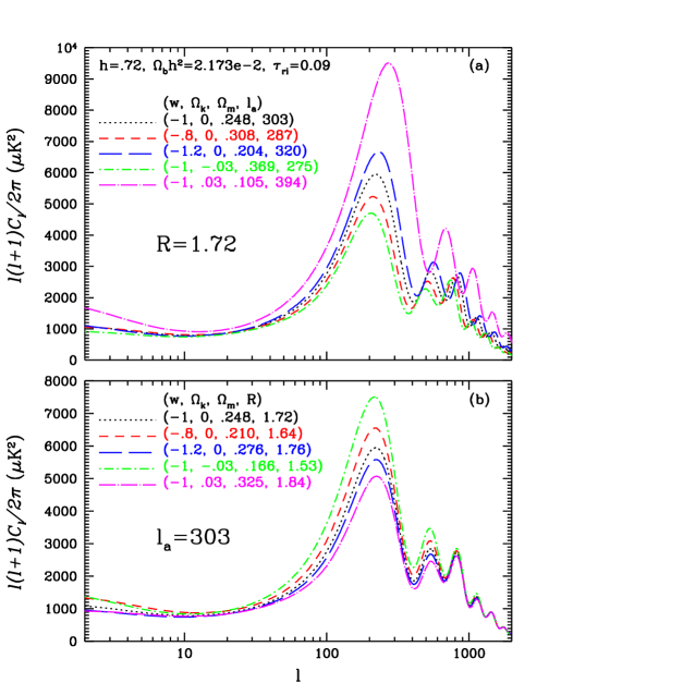
Figure 3: CMB angular power spectra for dark energy models that give the same values of $R$ or $l_{a}$.

Now we illustrate how using both $R$ and $l_{a}$ helps constrain models with a constant dark energy equation of state, and zero or small curvature (the class of models shown in Fig.3). Fig.4 shows the expected $R$, $l_{a}$ and $r_{s}(z_{CMB})$ as functions of $\Omega_{m}$ for five models. For reference, the values for $h$ and $\Omega_{b}h^{2}$ have been chosen such that the cosmological constant model satisfies both the $R$ and $l_{a}$ constraints from WMAP three year data at the same value of $\Omega_{m}$ (as in Fig.3). Note that for the other four models, the $R$ and $l_{a}$ constraints cannot be satisfied at the same $\Omega_{m}$ value. This is because $R$ and $r_{s}(z_{CMB})$ have different dependences on $\Omega_{m}$. Models that give the wrong $R$ and $r_{s}(z_{CMB})$ values can give the right value for $l_{a}$ because $l_{a}\propto R/r_{s}(z_{CMB})$. Using both $R$ and $l_{a}$ constraints thus helps tighten the constraint on $\Omega_{m}$, which leads to tightened constraints on $w$ or $\Omega_{k}$.

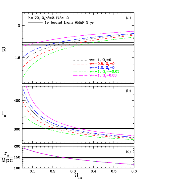
Figure 4: The expected $R$ and $l_{a}$ as functions of curvature for five simple dark energy models (with the same line types as in Fig.3).

When more complicated dark energy models and nonzero cosmic curvature are considered, there is a degeneracy between dark energy density function $X(z)$ and curvature. The $R$ or $l_{a}$ constraints from CMB can always be satisfied with a suitable choice of curvature, but satisfying the $R$ and the $l_{a}$ constraints usually require different values for curvature. Thus using both $R$ and $l_{a}$ constraints from CMB helps break the degeneracy between dark energy parameters and curvature. Fig.5 demonstrates this by showing the expected $R$, $l_{a}$, and $r_{s}(z_{CMB})$ as functions of curvature for the dark energy models from Fig.1 (with the same line types). For reference, the values for $\Omega_{m}$ and $h$ have been chosen such that the cosmological constant model satisfies both the $R$ and $l_{a}$ constraints from WMAP three year data. Clearly, the $R$ constraint rules out closed models with large curvature, while the $l_{a}$ constraint rules out open models with large curvature. The vertical dotted lines indicate the 1 $\sigma$ range of $\Omega_{k}$ from $R$, $l_{a}$, and $\Omega_{b}h^{2}$ constraints from WMAP three year data, combined with the data of 182 SNe Ia, and the SDSS BAO measurement.

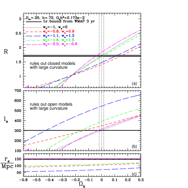
Figure 5: The expected $R$ and $l_{a}$ as functions of curvature for the dark energy models from Fig.1 (with the same line types). Both $R$ and $l_{a}$ are needed to constrain cosmic curvature.

Note that the baryon density $\Omega_{b}h^{2}$ should be included as an estimated parameter in the data analysis. This is because the value of $\Omega_{b}h^{2}$ is required in making a prediction for $l_{a}$ in a given dark energy model (see Eq.[3]), and it is correlated with $l_{a}$ (see Table II).

To summarize, we recommend that the covariance matrix of ($R$, $l_{a}$, $\Omega_{b}h^{2}$) given in Tables.I-II be used in the data analysis. To implement this, simply add the following term to the $\chi^{2}$ of a given model with $p_{1}=R$, $p_{2}=l_{a}$, and $p_{3}=\Omega_{b}h^{2}$:

$$\chi^{2}_{CMB}=\Delta p_{i}\left[Cov^{-1}(p_{i},p_{j})\right]\Delta p_{j},\hskip 14.22636pt\Delta p_{i}=p_{i}-p_{i}^{data},$$ (10)

where $p_{i}^{data}$ are the mean values given in Table I. The covariance matrix $Cov(p_{i},p_{j})$ is obtained by multiplying the normalized covariance matrix in Table II with $[Var(p_{i})\,Var(p_{j})]^{1/2}$, with the rms variance $[Var(p_{i})]^{1/2}$ given in Table I. Note that our constraints on ($R$, $l_{a}$, $\Omega_{b}h^{2}$) have been marginalized over all other parameters including the dark energy parameters.

As a test for the effectiveness of our simple method for incorporating CMB data, we derived the constraints on $w_{X}(z)=w$ (constant) and $w_{X}(z)=w_{0}+w_{a}(1-a)$ using ($R$, $l_{a}$, $\Omega_{b}h^{2}$), and compared with the results from using the full CMB code CAMB. For both sets of calculations, we assumed the same flat priors of $-2\leq w\leq 0$, $-2\leq w_{0}\leq 0$, and $-6\leq w_{a}\leq 3$, since $w$ and ($w_{0}$,$w_{a}$) are not well constrained by using CMB data alone. The pdf’s of $w$ and ($w_{0}$,$w_{a}$) span the entire allowed ranges, and have similar shapes in the two methods. We did not assume any priors on $H_{0}$ since we want to study CMB data only. For $w_{X}(z)=w$ (constant), using ($R$, $l_{a}$, $\Omega_{b}h^{2}$) gives $w=-0.96\pm 0.57$, while the full CMB code CAMB gives $w=-0.97\pm 0.53$. Using ($R$, $l_{a}$, $\Omega_{b}h^{2}$) $w_{0}=-1.0\pm 0.6$ and $w_{a}=-2.2\pm 2.1$, while the full CMB code CAMB gives $w_{0}=-0.9\pm 0.6$ and $w_{a}=-2.4\pm 2.0$. These comparisons indicate that our simple method of incorporating CMB data by using Eq.(10) is indeed efficient and appropriate as far as dark energy constraints are concerned. Since CMB data alone do not place tight constraints on dark energy, it is not appropriate to do the comparison of our method with the full CMB code for dark energy models with more parameters.

III.2 Constraints on dark energy

Because of our ignorance of the nature of dark energy, it is important to make model-independent constraints by measuring the dark energy density $\rho_{X}(z)$ as a free function. Measuring $\rho_{X}(z)$ has advantages over measuring dark energy equation of state $w_{X}(z)$ as a free function; $\rho_{X}(z)$ is more closely related to observables, hence is more tightly constrained for the same number of redshift bins used Wang & Garnavich (2001); Tegmark (2002); Wang & Freese (2006). More importantly, measuring $w_{X}(z)$ implicitly assumes that $\rho_{X}(z)$ does not change sign in cosmic time (as $\rho_{X}(z)$ is given by the exponential of an integral over $1+w_{X}(z)$); this precludes whole classes of dark energy models in which $\rho_{X}(z)$ becomes negative in the future (“Big Crunch” models, see Linde (2004) for an example)Wang & Tegmark (2004).

We have reconstructed the dark energy density function $X(z)\equiv\rho_{X}(z)/\rho_{X}(0)$ by measuring its value at $z_{i}=z_{cut}(i/3)$ (i=1, 2, 3) at $z\leq z_{cut}$, and parametrized it by either a powerlaw ($X(z)\propto(1+z)^{\alpha}$) or an exponential function ($X(z)\propto e^{\alpha z}$) at $z>z_{cut}$ (see Eqs.(8)-(9)). We have chosen $z_{cut}=1.4$ as few SNe Ia have been observed beyond this redshift. We find that current data allow $\alpha>0$ for $X(z)\propto(1+z)^{\alpha}$ at $z>z_{cut}$, and require $\alpha<0$ for $X(z)\propto e^{\alpha z}$ at $z>z_{cut}$. This means that assuming powerlaw dark energy at early times allows significant amount of dark energy at $z\gg 1$, while assuming exponential dark energy at early times is equivalent to postulating dark energy that disappears at $z\gg 1$. The latter is more physically sensible since dark energy is introduced to explain late time cosmic acceleration. Introducing dark energy that is important at early times could cause problems with Big Bang Nucleosynthesis Steigman (2006) and formation of cosmic large scale structure Sandvik (2004).

Fig.6 shows the reconstructed dark energy density function $X(z)$ using ($R$, $l_{a}$, $\Omega_{b}h^{2}$) from the three-year WMAP data, together with 182 SNe Ia and SDSS BAO measurement. The apparent shrinking of the error contours at $z>z_{cut}$ is due to the use of one parameter to describe $X(z)$ at $z>z_{cut}$. Future theoretical work and better data will allow better-motivated description of dark energy at early times. Fig.7 shows the corresponding constraints on the cosmic expansion history $H(z)$.

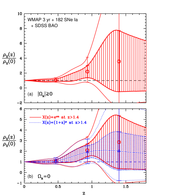
Figure 6: Constraints on dark energy density using $R$, $l_{a}$, and $\Omega_{b}h^{2}$ from the three-year WMAP data, together with 182 SNe Ia and SDSS BAO measurement. The shaded areas indicate the 68% confidence regions, while the outside contours bound the 95% confidence regions.

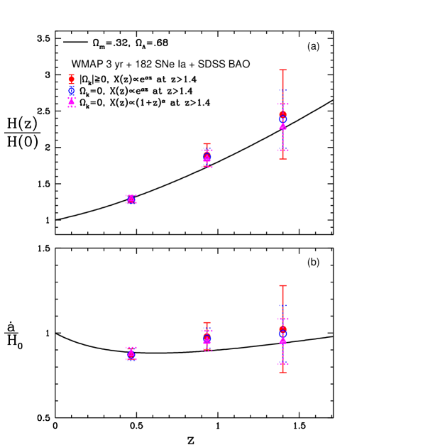
Figure 7: Constraints on the expansion history of the universe $H(z)$ that corresponds to Fig.6, using $R$, $l_{a}$, and $\Omega_{b}h^{2}$ from the three-year WMAP data, together with 182 SNe Ia and SDSS BAO measurement. The error bars indicate the 68% confidence intervals.

For a flat universe, the dark energy constraints at $z\leq 1$ are nearly independent of the early time assumption about dark energy, while the dark energy constraint at $z\sim z_{cut}$ is more stringent if $X(z)\propto(1+z)^{\alpha}$ at $z>z_{cut}$. This is as expected. Because of parameter correlations, stronger assumption about early time dark energy (the powerlaw form) leads to more stringent dark energy constraint at late times around $z\sim z_{cut}$.

Without assuming a flat universe, in the $X(z)\propto(1+z)^{\alpha}$ at $z>z_{cut}$ case, there is a strong degeneracy between curvature and the powerlaw index $\alpha$. This is as expected since the curvature contribution to the total matter-energy density is also a powerlaw, $(1+z)^{2}$. $X(z)$ is not well constrained in this case, and is not shown in Fig.6. When $X(z)\propto e^{\alpha z}$ is assumed at $z>z_{cut}$, there is no degeneracy between the exponential index $\alpha$ and curvature. $X(z)$ is well constrained in this case (see Fig.6).

For comparison with the work by others, Fig.8 shows the constraints on $(w_{0},w_{a})$ for models with dark energy equation of state $w_{X}(z)=w_{0}+w_{a}(1-a)$, using $R$, $l_{a}$, and $\Omega_{b}h^{2}$ from the three-year WMAP data, together with 182 SNe Ia and SDSS BAO measurement. These are consistent with the results of Zhao (2007); Wright (2007). Note that using $w_{X}(z)=w_{0}+w_{a}(1-a)$ implies extrapolation of dark energy to early times, which leads to artificially strong constraints (compared to model-independent constraints) on dark energy at both early and late times. This was noted by Riess (2007) as well.

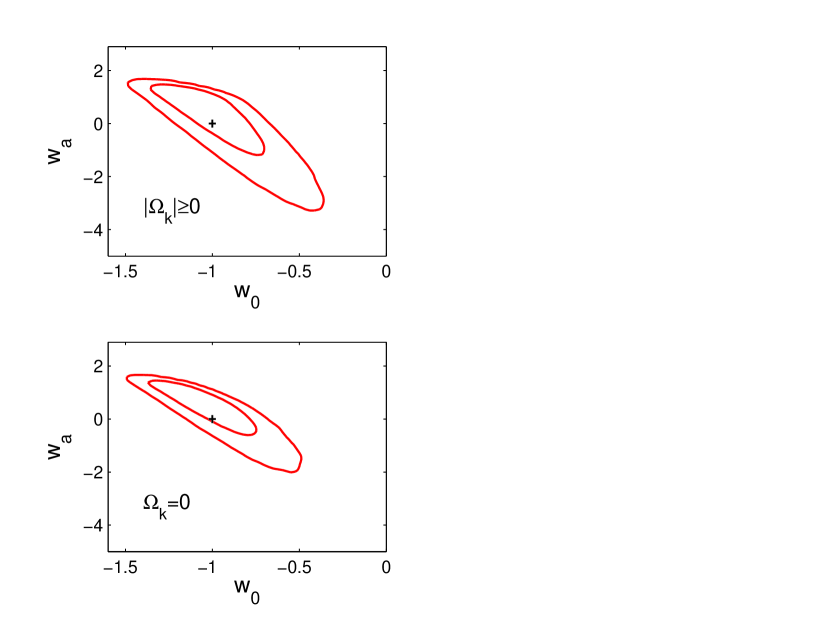
Figure 8: Constraints on $(w_{0},w_{a})$ using $R$, $l_{a}$, and $\Omega_{b}h^{2}$ from the three-year WMAP data, together with 182 SNe Ia and SDSS BAO measurement. The 68% and 95% confidence contours are shown.

Comparing Fig.6-8 with Figs.3-5 of Wang & Mukherjee (2006) (for the case of assuming $X(z)\propto(1+z)^{\alpha}$ at $z>z_{cut}$), it is clear that the constraints on dark energy have significantly tightened if a flat universe is assumed.

III.3 Cosmic curvature and dark energy constraints

Fig.9 shows the probability distribution function of cosmic curvature for different assumptions about dark energy: the model-independent dark energy density $\rho_{X}(z)$ reconstructed in the last subsection, the two parameter dark energy model $w_{X}(z)=w_{0}+w_{a}(1-a)$, and a constant dark energy equation of state. A flat universe is allowed at the 68% confidence level in all the cases when curvature is well constrained. $\Omega_{k}=-0.006_{-0.012}^{+0.013}$${}_{-0.025}^{+0.025}$ for assuming that $w_{X}(z)$ is constant, and $\Omega_{k}=-0.002_{-0.018}^{+0.018}$${}_{-0.032}^{+0.041}$ for $w_{X}(z)=w_{0}+w_{a}(1-a)$ (68% and 95% confidence levels). Assuming a constant dark energy equation of state gives the most stringent constraints on cosmic curvature. The bounds on cosmic curvature are less stringent if dark energy density is allowed to be a free function of redshift, and are dependent on the assumption about the early time property of dark energy. If dark energy is assumed to be an exponential function at $z>z_{cut}$ ($z_{cut}=1.4$), it is well constrained by current observational data (see Fig.6) and negligible at early times. In this case, curvature is well constrained as well. If dark energy is assumed to be a powerlaw at early times, its powerlaw index is strongly degenerate with curvature, and neither is well constrained.

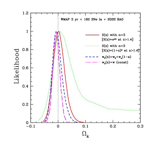
Figure 9: The probability distribution function of cosmic curvature for different assumptions about dark energy: the model-independent dark energy density $\rho_{X}(z)$ reconstructed in the last subsection, the two parameter dark energy model $w_{X}(z)=w_{0}+w_{a}(1-a)$, and a constant dark energy equation of state.

IV Summary and Discussion

We have presented a simple and effective method for incorporating constraints from CMB data into an analysis of other cosmological data (for example, SNe Ia and galaxy survey data), when constraining dark energy without assuming a flat universe.

We find that three-year WMAP data give constraints on $(R,l_{a},\Omega_{b}h^{2},\Omega_{m}h^{2},r_{s}(z_{CMB}),r(z_{CMB}))$ that are independent of the assumption about dark energy (see Table I). The constraints on ($\Omega_{m}h^{2},r_{s}(z_{CMB}),r(z_{CMB}))$) are also independent of the assumption about cosmic curvature, but they are strongly correlated with each other and are not suitable for use in constraining dark energy (see Table II).

We show that there are two CMB shift parameters, $R\equiv\sqrt{\Omega_{m}H_{0}^{2}}\,r(z_{CMB})$ (the scaled distance to recombination) and $l_{a}\equiv\pi r(z_{CMB})/r_{s}(z_{CMB})$ (the angular scale of the sound horizon at recombination); these retain the sensitivity to dark energy and curvature of $r(z_{CMB})$ and $r_{s}(z_{CMB})$, and have measured values that are nearly uncorrelated with each other (see Table II). We give the covariance matrix of ($R$, $l_{a}$, $\Omega_{b}h^{2}$) from the WMAP three year data (see Tables I and II).

We demonstrate that ($R$, $l_{a}$, $\Omega_{b}h^{2}$) provide an efficient summary of CMB data as far as dark energy constraints are concerned, and an intuitive way of understanding what the CMB does in terms of parameter constraints (see Figs.3-5).

While completing our paper (based on detailed calculations that have taken several months), we became aware of Ref.Elgaroy (2007). They also found that using both $R$ and $l_{a}$ tightens dark energy constraints. However, their paper assumed a flat universe, and used an approximation for $l_{a}$ that ignores both curvature and dark energy contributions. We use the exact expression for $l_{a}$ and derived the covariance matrix for ($R$, $l_{a}$, $\Omega_{b}h^{2}$) which are based on the MCMC chains from our full CMB power spectrum calculations without assuming spatial flatness.

We have used ($R$, $l_{a}$, $\Omega_{b}h^{2}$) from WMAP three year data, together with 182 SNe Ia (from the HST/GOODS program, the first year Supernova Legacy Survey, and nearby SN Ia surveys), and SDSS measurement of the baryon acoustic oscillation scale in deriving constraints on dark energy. Assuming the HST prior of $H_{0}=72\pm 8\,$(km/s)Mpc^-1 HST_H0 (2001), we find that current observational data provide significantly tightened constraints on dark energy models in a flat universe, and less stringent constraints on dark energy without assuming spatial flatness (see Figs.6-8). Dark energy density is consistent with a constant in cosmic time, with marginal deviations from a cosmological constant that may reflect current systematic uncertainties or true evolution in dark energy (see Figs.6-7). Our findings are consistent with that of Riess (2007) and Davis (2007).

A flat universe is allowed by current data at the 68% confidence level. As expected, the bounds on cosmic curvature are less stringent if dark energy density is allowed to be a free function of cosmic time, and are also dependent on assumption about dark energy properties at early times (see Fig.9). The behavior of dark energy at late times (where it causes cosmic acceleration and is directly probed by SN Ia data) and at early times (where it is poorly constrained) should be separated in parameter estimation in order to place robust constraints on dark energy and cosmic curvature (see Sec.IIIB and C).

Future dark energy experiments from both ground and space Wang (2000a); deft (2006); ground (2007); jedi (2006), together with CMB data from Planck planck (2007), will dramatically improve our ability to probe dark energy, and eventually shed light on the nature of dark energy.

Acknowledgements We thank Jan Michael Kratochvil for being a strong advocate of marginalizing SN Ia data over $H_{0}$; Savas Nesseris, Leandros Perivolaropoulos, and Andrew Liddle for useful discussions. We gratefully acknowledge the use of camb and cosmomc. This work was supported in part by NSF CAREER grants AST-0094335 (YW). PM is funded by PPARC (UK).

Appendix A Marginalization over $H_{0}$ in SN Ia flux statistics

Because of calibration uncertainties, SN Ia data need to be marginalized over $H_{0}$ if SN Ia data are combined with data that are sensitive to the value of $H_{0}$. This is the case here (see the next section). We use the angular scale of the sound horizon at recombination $l_{a}$ which depends on $\Omega_{m}h^{2}$, while the dimensionless Hubble parameter $E(z)=H(z)/H_{0}$ (which appears in the derivation of all distance-redshift relations) depends on $\Omega_{m}$. Hence a dependence on $H_{0}$ is implied. We marginalize the SN Ia data over $H_{0}$ while imposing a prior of $H_{0}=72\pm 8\,$(km/s)Mpc^-1 from HST Cepheid varibale star observations HST_H0 (2001).

The marginalization of SN Ia data over $H_{0}$ was derived in Wang & Garnavich (2001) for the usual magnitude statistics (assuming that the intrinsic dispersion in SN Ia peak brightness is Gaussian in magnitudes). Here we present the formalism for marginalizing SN Ia data over $H_{0}$ in the flux-averaging of SN Ia data using flux statistics (see Eq.[11]). The public software for implementing SN Ia flux averaging with marginalization over $H_{0}$ (compatible with cosmomc) is available at http://www.nhn.ou.edu/$\sim$wang/SNcode/.

Flux-averaging of SN Ia data Wang (2000) is needed to minimize the systematic effect of weak lensing of SNe Ia lensing (1998). Wang & Mukherjee (2004) presented a consistent framework for flux-averaging SN Ia data using flux statistics. Normally distributed measurement errors are required if the $\chi^{2}$ parameter estimate is to be a maximum likelihood estimator (Press et al., 1994). Hence, if the intrinsic dispersion in SN Ia peak brightness is Gaussian in flux, we have

$$\chi^{2}_{N_{data}}(\mbox{\bf s})=\sum_{i}\frac{\left[F(z_{i})-F^{p}(z_{i}|\mbox{\bf s})\right]^{2}}{\sigma_{F,i}^{2}}.$$ (11)

Since the peak brightness of SNe Ia have been given in magnitudes with symmetric error bars, $m_{peak}\pm\sigma_{m}$, we obtain equivalent errors in flux:

$$\sigma_{F}\equiv\frac{F(m_{peak}+\sigma_{m})-F(m_{peak}-\sigma_{m})}{2}.$$

After flux-averaging, we have

$$\chi^{2}=\sum_{i}\frac{\left[\overline{F}(\overline{z}_{i})-F^{p}(\overline{z}_{i}|\mbox{\bf s})\right]^{2}}{\sigma_{\overline{F},i}^{2}},$$ (12)

where $F^{p}(\overline{z}_{i}|\mbox{\bf s}_{1})=\left(d_{L}(\overline{z}_{i}|\mbox{\bf s})/\mbox{Mpc}\right)^{-2}$.

The predicted SN Ia flux $F^{p}(z_{i}|\mbox{\bf s})=\left[d_{L}(z_{i}|\mbox{\bf s})/{\rm Mpc}\right]^{-2}\propto h^{2}$. Assuming that the dimensionless Hubble parameter $h$ is uniformly distributed in the range [0,1], it is straightforward to integrate over $h$ in the probability distribution function to obtain

$$p(\mbox{\bf s}|0\leq h\leq 1)=e^{-\chi^{2}/2}=\frac{\int_{0}^{1}dx\,e^{-g(x)}}{\int_{0}^{1}dx\,e^{-g_{0}(x)}}$$ (13)

where

$$g(x)\equiv\sum_{i}\frac{\left[\overline{F}(\overline{z}_{i})-x^{2}F^{p}_{*}(\overline{z}_{i}|\mbox{\bf s})\right]^{2}}{2\sigma_{\overline{F},i}^{2}},$$

$$g_{0}(x)\equiv(x^{2}-1)^{2}\sum_{i}\frac{\overline{F}(\overline{z}_{i})^{2}}{2\sigma_{\overline{F},i}^{2}},$$ (14)

where $F^{p}_{*}(\overline{z}_{i}|\mbox{\bf s})=F^{p}(\overline{z}_{i}|\mbox{\bf s},h=1)$.

References

- Riess et al. (1998) Riess, A. G, et al., 1998, Astron. J., 116, 1009
- Perlmutter et al. (1999) Perlmutter, S. et al., 1999, ApJ, 517, 565
- Freese et al. (1987) Freese, K., Adams, F.C., Frieman, J.A., and Mottola, E., Nucl. Phys. B287, 797 (1987).
- Linde (1987) Linde A D, “Inflation And Quantum Cosmology,” in Three hundred years of gravitation, (Eds.: Hawking, S.W. and Israel, W., Cambridge Univ. Press, 1987), 604-630.
- Peebles & Ratra (1988) Peebles, P.J.E., and Ratra, B., 1988, ApJ, 325, L17
- Wetterich (1988) Wetterich, C., 1988, Nucl.Phys., B302, 668
- Frieman et al. (1995) Frieman, J.A., Hill, C.T., Stebbins, A., and Waga, I., 1995, PRL, 75, 2077
- Caldwell, Dave & Steinhardt (1998) Caldwell, R., Dave, R., & Steinhardt, P.J., 1998, PRL, 80, 1582
- Sahni & Habib (1998) Sahni, V., & Habib, S., 1998, PRL, 81, 1766
- Parker & Raval (1999) Parker, L., and Raval, A., 1999, PRD, 60, 063512
- Boisseau et al. (2000) Boisseau, B., Esposito-Farèse, G., Polarski, D. & Starobinsky, A. A. 2000, Phys. Rev. Lett., 85, 2236
- Dvali, Gabadadze, & Porrati (2000) Dvali, G., Gabadadze, G., & Porrati, M. 2000, Phys.Lett. B485, 208
- Mersini, Bastero-Gil, & Kanti (2001) Mersini, L., Bastero-Gil, M., & Kanti, P., 2001, PRD, 64, 043508
- Freese & Lewis (2002) Freese, K., & Lewis, M., 2002, Phys. Lett. B, 540, 1
- Padmanabhan (2003) Padmanabhan, T., 2003, Phys. Rep., 380, 235
- Peebles & Ratra (2003) Peebles, P.J.E., & Ratra, B., 2003, Rev. Mod. Phys., 75, 559
- Carroll et al. (2004) Carroll, S M, de Felice, A, Duvvuri, V, Easson, D A, Trodden, M & Turner, M S, Phys.Rev. D71 (2005) 063513
- Onemli & Woodard (2004) Onemli, V. K., & Woodard, R. P. 2004, Phys.Rev. D70, 107301
- Cardone et al. (2005) Cardone, V.F., Tortora, C., Troisi, A., & Capozziello, S. 2005, astro-ph/0511528, Phys.Rev.D, in press
- Kolb, Matarrese, & Riotto (2005) Kolb, E.W., Matarrese, S., & Riotto, A. 2005, astro-ph/0506534
- Caldwell (2006) Caldwell, R.R.; Komp, W.; Parker, L.; Vanzella, D.A.T., Phys.Rev. D73 (2006) 023513
- Kahya & Onemli (2006) E. O. Kahya and V. K. Onemli, gr-qc/0612026
- DeFelice (2007) De Felice, A.; Mukherjee, P.; Wang, Y., PRD, submitted (2007), arXiv:0706.1197 [astro-ph]
- Koi (2007) Koivisto, T.; Mota, D.F., hep-th/0609155, Phys.Rev. D75 (2007) 023518
- Ng (2007) Ng, Y.J., gr-qc/0703096
- Wang & Tegmark (2004) Wang, Y., & Tegmark, M. 2004, Phys. Rev. Lett., 92, 241302
- Wang & Tegmark (2005) Wang, Y., & Tegmark, M. 2005, Phys. Rev. D 71, 103513
- Alam & Sahni (2005) Alam, U., & Sahni, V. 2005, astro-ph/0511473
- Daly & Djorgovski (2005) Daly,R. A.,& Djorgovski, S. G. 2005, astro-ph/0512576.
- Jassal, Bagla, & Padmanabhan (2005a) Jassal, H.K., Bagla, J.S., Padmanabhan, T. 2005, Phys.Rev.D 72, 103503
- Jassal, Bagla, & Padmanabhan (2005b) Jassal, H.K., Bagla, J.S., Padmanabhan, T. 2005, Mon.Not.Roy.Astron.Soc.Letters, 356, L11
- Barger (2006) Barger, V.; Gao, Y.; Marfatia, D., astro-ph/0611775
- Dick, Knox, & Chu (2006) Dick, J., Knox, L., & Chu, M. 2006, astro-ph/0603247
- Huterer (2006) Huterer, D.; Peiris, H.V., astro-ph/0610427
- Jassal, Bagla, & Padmanabhan (2006) Jassal, H.K., Bagla, J.S., Padmanabhan, T. 2006, astro-ph/0601389
- Liddle (2006) Liddle, A.R.; Mukherjee, P.; Parkinson, D.; Wang, Y., PRD, 74, 123506 (2006), astro-ph/0610126
- Nesseris & Perivolaropoulos (2006) Nesseris, S., & Perivolaropoulos, L. 2006, astro-ph/0602053; Nesseris, S., & Perivolaropoulos, L. 2006, astro-ph/0612653
- Schimd et al. (2006) Schimd, C. et al. 2006, astro-ph/0603158
- Sumu (2006) Samushia, L.; Ratra, B., Astrophys.J. 650 (2006) L5
- Wilson, Chen, & Ratra (2006) Wilson, K.M., Chen, G., Ratra, B. 2006, astro-ph/0602321
- Xia (2006) Xia, J.-Q.; Zhao, G.-B.; Li, H.; Feng, B.; Zhang, X., Phys.Rev. D74 (2006) 083521
- Alam (2007) Alam, U.; Sahni, V.; Starobinsky, A.A., astro-ph/0612381, JCAP 0702 (2007) 011
- Davis (2007) Davis, T. M., et al. 2007, astro-ph/0701510
- Wei (2007) Wei, H.; Zhang, S.N., astro-ph/0609597, Phys.Lett. B644 (2007) 7
- Zhang (2007) Zhang, J.; Zhang, X.; Liu, H., astro-ph/0612642
- Zun (2007) Zunckel, C.; Trotta, R., astro-ph/0702695
- sdss (2004) Tegmark, M., et al. 2004, ApJ, 606, 702
- 2df (2006) Verde, L., et al., 2002, MNRAS, 335, 432; Hawkins, E., et al. 2003, MNRAS, 346, 78
- Polarski & Ranquet (2005) D. Polarski, and A. Ranquet, Phys. Lett. B627, 1 (2005) [astro-ph/0507290]
- Franca (2006) U. Franca, Phys. Lett. B 641, 351 (2006) [arXiv:astro-ph/0509177]
- Ichikawa & Takahashi (2006) K. Ichikawa and T. Takahashi, Phys. Rev. D73, 083526 (2006) [arXiv:astro-ph/0511821]
- Ichikawa et al. (2006) K. Ichikawa, M. Kawasaki, T. Sekiguchi and T. Takahashi, JCAP 0612, 005 (2006) [arXiv:astro-ph/0605481]
- Clarkson (2007) Clarkson, C.; Cortes, M.; Bassett, B.A., astro-ph/0702670
- Gong (2007) Gong, Y.; Wang, A., astro-ph/0612196, Phys.Rev. D75 (2007) 043520
- Ichikawa (2007) Ichikawa, K.; Takahashi, T., stro-ph/0612739, JCAP 0702 (2007) 001
- Wright (2007) Wright, E.L., astro-ph/0701584
- Zhao (2007) Zhao, G., et al., astro-ph/0612728
- Fixsen (1996) Fixsen, D. J., 1996, ApJ, 473, 576
- Eisenstein & Hu (1998) Eisenstein, D. & Hu, W. 1998, ApJ, 496, 605
- Page (2003) Page, L., et al. 2003, ApJS, 148, 233
- Spergel et al. (2006) Spergel, D.N., et al. 2006, astro-ph/0603449, ApJ, in press
- Riess (2007) Riess, A.G., et al., astro-ph/0611572
- Wood (2007) Wood-Vasey, W. M., et al., astro-ph/0701041
- Wang (2000) Wang, Y., ApJ 536, 531 (2000)
- Astier et al. (2005) Astier, P., et al. 2005, astro-ph/0510447, Astron. Astrophys. 447 (2006) 31
- Eisenstein et al. (2005) Eisenstein, D., et al., ApJ, 633, 560
- Lewis02 (2002) Lewis, A., & Bridle, S. 2002, PRD, 66, 103511
- WMAP (2006) http://lambda.gsfc.nasa.gov/product/map/current/
- Lewis, Challinor, & Lasenby (2000) Lewis, A., Challinor, A., and Lasenby, A., Astrophys. J., 538, 473. See http://camb.info.
- Chev01 (2001) Chevallier, M., & Polarski, D. 2001, Int. J. Mod. Phys. D10, 213
- HST_H0 (2001) Freedman, W. L., et al. 2001, ApJ, 553, 47
- Bond (1997) Bond, J. R., Efstathiou, G., & Tegmark, M. 1997, MNRAS, 291, L33
- Odman et al. (2003) Odman, C.J., Melchiorri, A., Hobson, M. P., & Lasenby, A. N. 2003, Phys.Rev. D67, 083511
- Wang & Mukherjee (2004) Wang, Y., & Mukherjee, P. 2004, ApJ, 606, 654
- Wang & Mukherjee (2006) Wang, Y., & Mukherjee, P. 2006, ApJ, 650, 1
- Wang & Garnavich (2001) Wang, Y., and Garnavich, P. 2001, ApJ, 552, 445
- Tegmark (2002) Tegmark, M. 2002, Phys. Rev. D66, 103507
- Wang & Freese (2006) Wang, Y., & Freese, K. 2006, Phys.Lett. B632, 449 (astro-ph/0402208)
- lensing (1998) Kantowski, R., Vaughan, T., & Branch, D. 1995, ApJ, 447, 35; Frieman, J. A. 1997, Comments Astrophys., 18, 323; Wambsganss, J., Cen, R., Xu, G., & Ostriker, J.P. 1997, ApJ, 475, L81; Holz, D.E. 1998, ApJ, 506, L1; Wang, Y. 1999, ApJ, 525, 651
- Press et al. (1994) Press, W.H., Teukolsky, S.A., Vettering, W.T., & Flannery, B.P. 1994, Numerical Recipes, Cambridge University Press, Cambridge.
- Elgaroy (2007) Elgaroy, O., and Multamaki, T., astro-ph/0702343.
- Wang (2000a) Wang, Y. 2000, ApJ 531, 676
- deft (2006) Albrecht, A.; Bernstein, G.; Cahn, R.; Freedman, W. L.; Hewitt, J.; Hu, W.; Huth, J.; Kamionkowski, M.; Kolb, E.W.; Knox, L.; Mather, J.C.; Staggs, S.; Suntzeff, N.B., Report of the Dark Energy Task Force, astro-ph/0609591
- ground (2007) See for example, http://www.astro.ubc.ca/LMT/alpaca/; http://www.lsst.org/; http://www.as.utexas.edu/hetdex/. deft (2006) contains a more complete list of future dark energy experiments.
- jedi (2006) Wang, Y., et al., BAAS, v36, n5, 1560 (2004); Crotts, A., et al. (2005), astro-ph/0507043; Cheng, E.; Wang, Y.; et al., Proc. of SPIE, Vol. 6265, 626529 (2006); http://jedi.nhn.ou.edu/
-
planck (2007)
Planck Bluebook,
http://www.rssd.esa.int/index.php?project=PLANCK - Steigman (2006) Steigman, G. 2006, astro-ph/0611209
- Sandvik (2004) Sandvik, H.; Tegmark, M.; Zaldarriaga, M.; Waga, I. 2004, Phys.Rev. D69 (2004) 123524
- Linde (2004) Wang, Y.; Kratochvil,J.M.; Linde, A.; Shmakova, M. 2004, JCAP, 12, 006 (2004), astro-ph/0409264
- Shafieloo et al. (2006) Shafieloo, A.; Alam, U.; Sahni, V.; and Starobinsky, A.A. 2005, MNRAS, 366, 1081