The Helium Abundance and $\Delta Y/\Delta Z$ in Lower Main Sequence Stars

Abstract

We use nearby K dwarf stars to measure the helium–to–metal enrichment ratio $\Delta Y/\Delta Z$, a diagnostic of the chemical history of the Solar Neighbourhood. Our sample of K dwarfs has homogeneously determined effective temperatures, bolometric luminosities and metallicities, allowing us to fit each star to the appropriate stellar isochrone and determine its helium content indirectly. We use a newly computed set of Padova isochrones which cover a wide range of helium and metal content.

Our theoretical isochrones have been checked against a congruous set of main sequence binaries with accurately measured masses, to discuss and validate their range of applicability. We find that the stellar masses deduced from the isochrones are usually in excellent agreement with empirical measurements. Good agreement is also found with empirical mass–luminosity relations.

Despite fitting the masses of the stars very well, we find that anomalously low helium content (lower than primordial helium) is required to fit the luminosities and temperatures of the metal poor K dwarfs, while more conventional values of the helium content are derived for the stars around solar metallicity.

We have investigated the effect of diffusion in stellar models and LTE assumption in deriving metallicities. Neither of these is able to resolve the low helium problem alone and only marginally if the cumulated effects are included, unless we assume a mixing-length which is strongly decreasing with metallicity. Further work in stellar models is urgently needed.

The helium–to–metal enrichment ratio is found to be $\Delta Y/\Delta Z=2.1\pm 0.9$ around and above solar metallicity, consistent with previous studies, whereas open problems still remain at the lowest metallicities. Finally, we determine the helium content for a set of planetary host stars.

1 Introduction

K dwarfs are long-lived stars and can be regarded as snapshots of the stellar populations formed at different times over the history of our Galaxy, therefore constituting an optimal tool for any study dealing with its chemical evolution (e.g. Kotoneva et al. 2002). K dwarfs share a similar metallicity distribution with the G dwarfs, in which most stars have metallicities around the solar value, a feature not expected in the simplest, closed-box models of Galactic chemical evolution (i.e. the G-dwarf problem). In addition to the abundance patterns of metals in a stellar population, the helium content $Y$ can also diagnose its chemical evolution, but this diagnostic has received less attention because measuring the helium content of low mass stars can only be done indirectly (e.g. Jimenez et al. 2003). Typically, one measures a differential production rate of the helium mass fraction $Y$ in the stellar population relative to the metal mass fraction $Z$, i.e. $\Delta Y/\Delta Z$. For the solar neighbourhood, Jimenez et al. (2003) determine $\Delta Y/\Delta Z\approx 2.1\pm 0.4$ from K dwarfs, a value similar to that found by studying H II regions in both the Milky Way and external galaxies (e.g. Balser 2006). Metals mainly come from supernovae with high-mass progenitors, whereas helium is also injected into the interstellar medium by mass-loss from intermediate and low mass stars : $\Delta Y/\Delta Z$ can thus be computed from stellar evolutionary theory for a given initial mass function (e.g. Chiosi & Matteucci 1982; Maeder 1992, 1993; Chiappini, Renda & Matteucci 2002). The ratio $\Delta Y/\Delta Z$ can also be used to infer the primordial helium abundance $Y_{P}$ by extrapolating to $Z=0$; the technique is usually applied to extragalactic H II regions – the K dwarfs studied here provide an independent check on $Y_{P}$. Cosmic Microwave Background measurements alone are not able to provide a tight constraint in $Y_{P}$ (Trotta & Hansen 2004), but WMAP3 data on the cosmic baryon density when combined with Standard Big Bang Nucleosynthesis returns a formally accurate value for $Y_{P}$ (see Section 4.2). Finally, age determinations for both resolved and integrated stellar populations typically assume a value for $\Delta Y/\Delta Z$, and accurately knowing the age of galaxies can, in turn, help to determine the nature of dark energy (Jimenez & Loeb 2002).

Helium lines are not easily detectable in the spectra of low mass stars, with the notable exception of hot horizontal branch objects, whose atmospheres are, however, affected by gravitational settling and radiative levitation, which strongly alter the initial chemical stratification (e.g. Michaud, Vauclair & Vauclair 1983; Moehler et al. 1999) and whose composition anyway would not reflect the original helium abundance at their birth. Therefore, assumptions have to be made for the initial helium content of models of low-mass stars. Very often, for the sake of simplicity, it is supposed that the metallicity $Z$ and helium fraction $Y$ are related through a constant ratio $\Delta Y/\Delta Z$. The latter is often determined from the result of the solar calibration $(Y_{\odot}-Y_{P})/Z_{\odot}$ and for any other star of known metallicity, the helium abundance is scaled to the solar one as $Y=Y_{\odot}+\frac{\Delta Y}{\Delta Z}\times(Z-Z_{\odot})$. Most of the conclusions drawn when comparing theoretical isochrones with binaries (e.g. Torres et al. 2002; Torres & Ribas 2002; Lacy et al. 2005; Torres et al. 2006; Boden, Torres & Latham 2006; Henry et al. 2006) and field stars (e.g. Allende Prieto & Lambert 1999; Valenti & Fischer 2005) thus reflect this tacit assumption on the helium content.

Recent results, however suggest that the naive assumption that $\Delta Y/\Delta Z$ varies linearly and with a universal law might not be correct. For example, the Hyades seem to be $Y$ deficient for their metallicity (Perryman et al. 1998; Lebreton, Fernandes & Lejeune 2001; Pinsonneault et al. 2003). The discovery that the Globular Cluster $\omega$ Cen has at least two different components of the main sequence and multiple turnoffs (Lee et al. 1999; Pancino et al. 2000, 2002; Ferraro et al. 2004; Bedin et al. 2004) can be explained assuming stellar populations with very different helium abundances (Norris 2004) and thus very different $\Delta Y/\Delta Z$. Recently, compelling evidence has been found for a helium spread among the main sequence in the Globular Clusters NGC 2808 (D’Antona et al. 2005a) and the blue horizontal branch stars in the Globular Cluster NGC 6441 (Caloi & D’Antona 2007). At the same time, for a different sample of Galactic Globular Clusters Salaris et al. (2004) found a very homogeneous value of $Y$ with practically no helium abundance evolution over the entire metallicity range spanned by their study. All this suggests that a patchy variation of $\Delta Y/\Delta Z$ and complex chemical evolution histories might be not so unusual in our Galaxy. Similar indications also start to appear for extragalactic objects (Kaviraj et al. 2007). There are various methods to infer the helium content in Globular Clusters (e.g. Sandquist 2000) and all take advantage of the fact that in these objects it is relatively easy to perform statistical analysis over large stellar populations.

The determination of the helium content in nearby field stars, on the contrary, is more challenging, because it is less straightforward to build a statistically large and homogeneously selected sample. Accurate parallaxes are needed and to avoid subtle reddening corrections only stars closer than $\sim 70$ pc must be used. All studies to date have exploited the fact that the broadening of the lower main sequence with metallicity effectively depends on the helium content (see Section 4) so that its width can be used to put constraints on $\Delta Y/\Delta Z$ (e.g. Faulkner 1967; Perrin et al. 1977; Fernandes, Lebreton & Baglin 1996; Pagel & Portinari 1998; Jimenez et al. 2003). In this work we take the same strategy, comparing the positions of a large sample of field stars with theoretical isochrones in the $M_{Bol}-T_{eff}$ plane. For the parameter space covered by the isochrones, the number of stars used, the accuracy and the homogeneity of the observational data (crucial when it comes to analyzing small differential effects in the HR diagram), this is the most extensive and stringent test on the helium content of lower main sequence stars undertaken to date.

An analogous work was pioneered by Perrin et al. (1977) with 138 nearby FGK stars but with much less accurate fundamental stellar parameters, pre-Hipparcos parallaxes and of course, older stellar models. After Hipparcos parallaxes become available, the problem was re-addressed by Lebreton et al. (1999) with a sample of 114 nearby FGK stars in the metallicity range $-1.0<\textrm{[Fe/H]}<0.3$, of which only 33 have $T_{eff}$ and $M_{bol}$ determined directly via the InfraRed Flux Method (hereafter IRFM) of Alonso et al. (1995, 1996a). For the remaining stars, temperatures were either recovered via spectroscopic methods or color indices and $M_{Bol}$ determined from the bolometric corrections of Alonso (1995, 1996b).

We have recently carried out a detailed empirical determination of fundamental stellar parameters via IRFM (Casagrande, Portinari & Flynn 2006) with the specific task of determining the helium content in dwarf stars by comparing them to theoretical isochrones. Our sample is similar in size to previous studies, but i) it has a larger metallicity coverage ii) we have improved the accuracy in the selection (see Section 2), iii) we have carefully and homogeneously determined the fundamental stellar parameters iv) focusing particularly on stars (K dwarfs) where the helium content can be most directly determined from the stellar structure models, since the effects of stellar evolution play an insignificant role.

Stellar models are common ingredients in a variety of studies addressing fundamental cosmological and astrophysical problems, from ages and evolution of galaxies, to complex stellar populations, to exoplanets. Nevertheless, our incomplete understanding of complex physical processes in stellar interior requires the introduction of free parameters that are calibrated to the Sun. Therefore, using main sequence nearby stars with accurate fundamental parameters to test the adequacy of extant stellar models is of paramount importance to validate their range of applicability (Lebreton 2000), as we do here.

The paper is organized as follows. In Section 2 we describe our sample and in Section 3 we present our theoretical isochrones and how they compare to observations. In Section 4 we delve into the derivation of the helium abundance for lower main sequence stars and in Section 5 we carefully analyze how the results depend on the assumptions made in stellar models. The applicability range of our results is obtained by comparing the prediction of the isochrones to a congruous set of main sequence binaries (Section 6) and to empirical mass-luminosity relations (Section 7). We suggest that an accurate mass-luminosity relation for metal poor dwarfs could actually put constraints on their helium content. In Section 8 we apply our method to derive masses and helium abundances for a small set of planet host stars. We finally conclude in Section 9.

2 Sample and Data selection

Our sample stems from the 104 GK dwarfs for which we computed accurate effective temperatures and bolometric luminosities via IRFM (Casagrande et al. 2006). For such stars accurate [$\alpha$/Fe] ratios and overall metallicities [M/H] are available from spectroscopy as described in more details in Casagrande et al (2006). The main metallicity parameter in theoretical models is in fact the total heavy-element abundance [M/H] and neglecting the $\alpha$ enhancement can lead to erroneous or biased conclusions (Gallart, Zoccali & Aparicio 2005). Once [M/H] is known, the metal mass fraction $Z$ can be readily computed (see Appendix A).

We also paid special attention to removing unresolved double/multiple and variable stars as described in full detail in Casagrande et al. (2006).

Some of the stars in the sample were too bright to have accurate 2MASS photometry and therefore the IRFM could not be applied. However, such stars have excellent $BV(RI)_{C}$ photometry so that from these colours it was possible to recover the effective temperature and bolometric flux by means of the multi-band calibrations given in Casagrande et al. (2006), homogeneously with the rest of the sample. In this manner twenty-three single (or well separated binary) and non variable stars were added to the sample. For these additional stars $T_{eff}$ and $\mathcal{F}_{Bol}(\textrm{earth})$ have been estimated averaging the values returned by the calibrations in all $BV(RI)_{C}$ bands. The standard deviation resulting from the values obtained in different bands has been adopted as a measure of the internal accuracy. The systematics due to the adopted absolute calibration (Figure 12 in Casagrande et al. 2006) have then been added to obtain the overall errors. When helium abundances for these additional stars are computed (Section 4), the resulting values are perfectly in line with those obtained for stars with fundamental parameters obtained via IRFM.

We remark that an accurate estimate of the absolute luminosity (or magnitude) of each star requires parallax accuracy at the level of a few percent. A possible limitation could be the Lutz & Kelker (1973) bias, however, as we discuss in Appendix B, when limiting our sample to parallaxes better than 6% the bias is negligible compared to other uncertainties. This requirement on the parallaxes reduces our sample to 105 stars (see Figure 3).

We derive the helium content of our stars indirectly by comparing their positions in the theoretical HR diagram with respect to a set of isochrones of different helium and metallicity content (see Section 4). If evolutionary effects have already taken place in stars, the comparison would be age dependent (see Section 3). However, for any reasonable assumption about the stellar ages, one can safely assume that all stars fainter than $M_{V}\sim 5.5$ are practically unaffected by evolution and lie close to their Zero Age Main Sequence (ZAMS) location (e.g. Fernandes et al. 1996; Pagel & Portinari 1998; Jimenez et al. 2003). In terms of $M_{Bol}$ the threshold is very similar (see figure 17 in Casagrande et al. 2006) so that we assume $M_{Bol}\geq 5.4$ as a conservative estimate : this reduces the sample to 86 K dwarfs.

For consistency with Casagrande et al. (2006), throughout the paper we assume $M_{Bol,\odot}=4.74$ and $L_{\odot}=3.842\times 10^{33}$ erg $s^{-1}$.

3 Theory

3.1 Fine structure in the HR diagram: the broadening of the Lower Main Sequence

Several effects are responsible for the observed width of the lower main sequence : among the physical ones are chemical composition, evolution and rotation whereas observational errors and undetected binarity among stars are spurious ones. We have carefully cleaned our sample from spurious effects (Casagrande et al. 2006) so here we discuss only the physical ones related to stellar structure.

The cut in absolute magnitudes adopted for our sample (Section 2) ensures that our stars have masses below solar. The location of the main sequence depends on the treatment of convection and the size of core convective regions only for stars with $M>1.1M_{\odot}$ and on rotation for stars with $M>1.4M_{\odot}$ (e.g. Fernandes et al. 1996) so these effects and the related theoretical uncertainties are of no concern to us.

It is known that young and fast rotating K dwarfs might exhibit color anomalies such as to alter their location on the HR diagram (e.g. Stauffer et al. 2003). However, as we discuss in Section 5.1 this is not of concern to us.

With typical masses $\sim 0.8\,M_{\odot}$ K dwarfs have lifetimes much longer than the present age of the Galactic disk (e.g. Jimenez, Flynn & Kotoneva 1998) and comparable to the present age of the Universe (Spergel et al. 2007) so that evolutionary effects do not need to be taken into account. For a given metallicity $Z$, an increase of $Y$ makes a given mass on the isochrone hotter and brighter so that the net result of varying $\Delta Y/\Delta Z$ is to affect the broadening of the lower main sequence (see Figures 3 and 4). Such behaviour can be explained in terms of quasi-homology relations (an increase of $Y$ in fact decreases the mean opacity and increases the mean molecular weight e.g. Cox & Giuli 1968; Fernandes et al. 1996) and it has been exploited by Pagel & Portinari (1998) and more recently by Jimenez et al. (2003) to put constraints on the local $\Delta Y/\Delta Z$.

3.2 Evolutionary tracks and isochrones

We have computed a series of stellar models, using the Padova code as in Salasnich et al. (2000). Since our sample includes only dwarfs, the evolutionary tracks are limited to the main sequence phase only. We consider a range of metallicities from $Z=0.0001$ to $Z=0.04$, and a range of $\Delta Y/\Delta Z$ between 0 and 6. Metal abundance ratios are taken from Grevesse & Noels (1993). The solar metallicity is fixed to be $Z_{\odot}=0.017$, which is the value preferred by Bertelli et al. (in preparation) to whom we refer for all details. With this $Z_{\odot}$, the model that reproduces the present solar radius and luminosity at an age of 4.6 Gyr was found to have $Y_{\odot}=0.263$, and $\alpha_{\rm MLT}=1.68$. These numbers imply $(Z/X)_{\odot}=0.0236$ which is slightly below the 0.0245 ratio quoted by Grevesse & Noels (1993). The difference between the adopted $(Z/X)_{\odot}=0.0236$ and the Grevesse & Noels (1993) ratio simply implies a shift in the zero-point of the solar calibration (from $Y_{\odot}=0.263$ to $0.289$) and it is of no concern as long as we are interested in the study of a differential quantity such as $\Delta Y/\Delta Z$. The adopted choice of $Y_{\odot}$ when combined with the latest $Y_{P}$ measurements (Section 4.2) formally returns a $\Delta Y/\Delta Z$ in the range $0.7-0.9$. Our choice is to have a solar model that fits well the solar position in the HR diagram (Figure 1), and is by no means intended to be an accurate re-calibration. The latter would in fact be possible only by including atomic diffusion in the solar model. Although in the Sun atomic diffusion is efficient, spectroscopic observations of stars in Galactic globular clusters and field halo stars (see discussion in Section 5.3.2) point to a drastically reduced efficiency of diffusion. For this reason, the effect of atomic diffusion is usually not included in the computation of large model grids (e.g. Pietrinferni et al. 2004; VandenBerg, Bergbusch, Dowler 2006) and the same approach is adopted here.

Figure 1: Comparison between 4.57 Gyr solar isochrone (age as determined from meteoritic measurements, Bahcall, Pinsonneault & Wasserburg 1995) and our sample stars in the [M/H] range $\pm 0.04$ dex around the solar value. In order to have conservatively small errors we have used only stars with parallaxes better than 3%. Transformations to plot the solar isochrone in the observational plane as discussed in Section 3.3. Overplotted is also the Sun ($\odot$) for which we have adopted colours and temperatures from Casagrande et al. (2006). The difference with the empirical $B-V$ of Holmberg et al. (2006) in unnoticeable. Interestingly in the theoretical plane there is a much tighter agreement between model and observations.

We also remark that the solar model is presently under profound revision after the updates in the estimated solar abundances (Asplund, Grevesse & Sauval, 2005) significantly diminish the agreement with helioseismology (e.g. Basu & Antia 2004; Antia & Basu 2005; Delahaye & Pinsonneault 2006). The present study however refers the “classic” solar model and metallicity as the zero-point calibration, and since the method relies on differential effects along the main sequence we do not expect that conclusions on $\Delta Y/\Delta Z$, which is a differential quantity, are significantly affected. Also, as already pointed out, the solar zero-point should be regarded as a calibration parameter and not as an absolutely determined value so that strong inferences on absolute values (among which $Y_{P}$) can hardly be drawn. Therefore, as we will see later, small errors in this calibration procedure, and especially in $Y_{\odot}$, are unlikely to affect our conclusions on the $\Delta Y/\Delta Z$ obtained for our sample of stars. Nonetheless, we caution on the hazardous comparison between the helium abundances deduced from the isochrones and external constraints such as the primordial helium abundance obtained with other techniques. In this case, in fact, differences in the zero-point of $Y_{\odot}$ does not cancel out anymore. We will return on the topic in Section 4.2.

The tracks computed cover the mass range between 0.15 and 1.5 $M_{\odot}$, which is far wider than needed for an analysis of our sample. Regarding convection, we adopt the same prescription as in Girardi et al. (2000): convective core overshooting is assumed to occur for stars with $M>1.0M_{\odot}$, with an efficiency $\Lambda_{c}=M/M_{\odot}-1.0$ (see Bressan et al. 1993 for the definition of $\Lambda_{c}$) that increases linearly with mass in the interval from 1 to 1.5 $M_{\odot}$. Lower mass stars are computed assuming the classical Schwarzschild criterion.

From these tracks, we can construct isochrones in the HR diagram for arbitrary ages, and any intermediate $Y(Z)$ relation, via simple linear interpolations within the grid of tracks.

Although our analysis is conducted using Padova isochrones, we have fully cross checked (Section 4) the results with an updated set of the MacDonald isochrones (Jimenez & MacDonald 1996; Jimenez et al. 2003) computed for a similar grid of values in $Y$ and $Z$. We have also compared our isochrones with other sets in the lower main sequence, namely the Teramo (Cordier et al. 2007) and Yonsei–Yale (Demarque et al. 2004) isochrones. The solar isochrone of each set is calibrated to reproduce the current position of the Sun in the HR diagram but the values of $Y_{\odot}$ and $Z_{\odot}$ are not identical, because of the different prescriptions and input physics implemented in various independent codes. As we have already pointed out, what matters is not the comparison between absolute values of $Y$ and $Z$. A meaningful comparison can only be done between isochrones of similar $\Delta Y/\Delta Z$ with respect to a common calibration point i.e. with respect to the solar isochrone. It is clear from Figure 2 that different set of isochrones are in general in good agreement. The agreement between Padova and Yale isochrones is outstanding throughout the entire range of metallicities and $M_{Bol}$ covered in this study. The comparison with the Teramo isochrones is also very good, except for the high metallicity isochrone that is significantly hotter in the Teramo dataset. At lower metallicities, the agreement with Teramo isochrones is always good except for the most metal poor and fainter stars in our sample. However, at luminosity higher than $M_{Bol}=6.0$ and below $\sim 4.5$ the agreement between Padova and Teramo isochrones is always outstanding. A more detailed comparison is outside the purpose of the paper, but clearly our results are not significantly affected by the particular set of isochrones used (see also Figure 7).

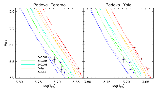
Figure 2: Left panel: comparison between Padova (thick dotted) and Teramo (thin continuous) isochrones. Both sets are calibrated on the Sun and the comparison at other metallicities $Z$ is done for similar value of $\Delta Y/\Delta Z\sim 1.4$. Also shown for comparison are the most metal poor (blue) and metal rich (red) stars in our sample. Right panel: same as left panel, but with respect to Yale (thin continuous lines) isochrones ($\Delta Y/\Delta Z\sim 2.0$)

3.3 Observational vs. theoretical plane

Comparison between model isochrones and data is usually done in the observational colour – absolute magnitude HR diagram rather than in its theoretical $T_{eff}$–$M_{Bol}$ counterpart. However, the observational plane makes use of the information extracted only from a limited part of the entire spectral energy distribution of a star (few thousands of Å  in the case of broad band colours, see also Section 5.1). Furthermore, for such a comparison theoretical isochrones have to be converted into colours and magnitudes via model atmospheres, introducing further model dependence and uncertainties (e.g. Weiss & Salaris 1999).

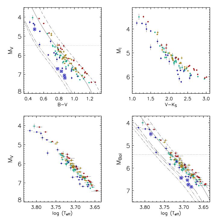
Figure 3: Comparison between observational, hybrid and theoretical planes. Parallax uncertainties are also included in error bars. Only stars with parallaxes better than 6% are shown. For the second panel ($M_{I},(V-K_{S})$) only stars with accurate IR photometry (“j_”$+$“h_”$+$ “k_msigcom”$<0.10$) are shown. Points correspond to the sample stars in the range $Z<0.007$ (blue), $0.007\leq Z<0.014$ (cyan), $0.014\leq Z<0.022$ (yellow), $Z\geq 0.022$ (red). Squares are intended to highlight stars with $Z\sim 0.001$ to facilitate comparison with metal poor isochrones. Overplotted are 1 Gyr isochrones of metallicity $Z=0.001$ (dot dashed), 0.017 (continuous) and 0.040 (dashed) under the standard assumption of $\Delta Y/\Delta Z=2$. The lower and upper $Z$ value roughly bracket the metallicity of our sample. Also shown for comparison (triple dot dashed) is an extremely helium poor isochrone ($Z=0.001$ and $Y=0.167$). In the fourth panel is also plotted an isochrone with $Z=0.004$ and $Y=0.250$ (long dashed line).

Sometimes the hybrid $T_{eff}$ – absolute magnitude plane is used although it has almost the same limitations as the observational one (the computation of absolute magnitudes from stellar models still requires the use of spectral libraries). In addition $T_{eff}$ is rarely empirically and consistently determined for all the stars, more often depending on the adopted colour–temperature transformation or resulting from a collection of inhomogeneous sources in literature. As a result, a single theoretical isochrone produces different loci in the color–magnitude diagram when different color-temperature relations are applied (e.g. Pinsonneault et al. 2004).

Working in the purely theoretical plane has many advantages. First, it is possible to directly compare observations to physical quantities such as temperature and luminosity (or equivalently $M_{Bol}$) predicted from stellar models. Secondly, for the purpose of this work, the effects of helium are highlighted in the theoretical plane, whereas in the widely used $(B-V)$ vs $M_{V}$ plane they are partly degenerate with the dependence of the colour index on metallicity (Castellani, Degl’Innocenti & Marconi 1999). Up to now, the drawback of working in the theoretical plane was that for a given set of stars, very rarely in literature homogeneous and accurate bolometric corrections and effective temperatures were available for large samples. However, for all our stars we have homogeneously derived $T_{eff}$ and bolometric luminosity from accurate multi–band photometry and basing on the IRFM (Section 2). In the case of K dwarfs $\sim$80% of the total luminosity is directly observed so that the dependence on model atmosphere is minimal.

The first feature that appears from the comparison between the observational $(B-V)$ and the theoretical HR diagram (Figure 3) is how in the $T_{eff}-M_{Bol}$ plane the separation between metal poor and metal rich stars is not as neat as in the observational $(B-V)$ counterpart. This was already noticed by Perrin et al. (1977) and Lebreton et al. (1999) and reflects the sensitivity of the $B,V$ colour indices to metallicity. To ensure this is not an artifact due to our temperature and/or luminosity scale, we also show a plot in the observational $M_{I}$ versus $(V-K_{S})$ plane. $(V-K_{S})$ is in fact and excellent temperature indicator with negligible dependence on metallicity and $M_{I}$ faithfully traces $M_{Bol}$ (Casagrande et al. 2006). The reduced separation between metal poor and metal rich stars is confirmed.

To quantify how strong is the effect of metallicity in the $(B-V)$ plane, we have drawn theoretical isochrones in this plane, too. The transformations to convert theoretical isochrones into the observational plane have been obtained by fitting the following formulae to the stars in Casagrande et al. (2006) (their figure 17):

$$BC=a_{0}+a_{1}T_{eff}+a_{2}T_{eff}^{2}+a_{3}T_{eff}\textrm{[M/H]}+a_{4}\textrm{[M/H]}$$

$$\phantom{BC=}+a_{5}\textrm{[M/H]}^{2}$$ (1)

where $BC$ is the bolometric correction (from which $M_{V}=M_{Bol}-BC$) and:

$$B-V=b_{0}+b_{1}T_{eff}+b_{2}T_{eff}^{2}+b_{3}T_{eff}\textrm{[M/H]}+b_{4}\textrm{[M/H]}$$

$$\phantom{B-V=}+b_{5}\textrm{[M/H]}^{2}.$$ (2)

Both transformations are accurate to 0.02 mag and the coefficients are given in Table 1.

Table 1: Coefficients $i=a,b$ for equation (1) and (2) in the temperature range $4300<T_{eff}<6700$ K.

	$i_{0}$	$i_{1}$	$i_{2}$	$i_{3}$	$i_{4}$	$i_{5}$
$BC$	$-7.67005$	0.00248	$-2$E$-7$	9E$-5$	$-0.44985$	0.00672
$B-V$	4.96959	$-0.00120$	$8$E$-8$	$-3$E$-5$	0.29112	0.03581

With this approach the comparison between isochrones and sample stars in the two planes does not depend on model atmospheres, since we use empirical conversions derived from the same sample stars. Notice though that the empirical conversions of Casagrande et al. (2006) show good agreement with theoretical ones from e.g. Kurucz or MARCS model atmospheres.

From Figure 3 is clear that for metallicity around and above the solar one, isochrones with $\Delta Y/\Delta Z=2$ are in overall good agreement with the data. On the contrary, a clear discrepancy appears for metal poor stars where the standard assumption $\Delta Y/\Delta Z=2$ returns isochrones that are too hot.

To achieve a match between the metal poor stars and the isochrone, we need to decrease the corresponding helium abundance down to $Y=0.167$, well below the primordial value expected from Big Bang nucleosynthesis. Even with such a radically low helium abundance the discrepancy is persistent. An alternative to reduced helium in the stars is to use a theoretical isochrone with a more orthodox helium abundance ($Y=0.250$, (fourth panel in Figure 3) but with a metallicity ($Z=0.004$) higher by $\sim 0.6$ dex (with respect to $Z=0.001$), a very large change in metallicity content indeed (and discussed in detail in Section 5.4). This comparison qualitatively illustrates how discrepant the lower metallicity stars are compared to models. This result is discussed in the detailed analysis of Section 4.

4 Helium abundance and mass from theoretical isochrones

In the previous Section we have shown that the most suitable place to estimate the effects of the helium content on the lower main sequence is the theoretical $T_{eff}-M_{Bol}$ plane. In this section we follow this by fitting to each star the most appropriate isochrone; the metallicity $Z$ of each star is known from its spectroscopic measurement (see also Appendix A) and we thereby determine its helium content $Y$. We thus differ from previous works which –by means of different techniques– focused on the overall comparison between theoretical predictions and observations along the lower main sequence (Fernandes et al. 1996; Pagel & Portinari 1998; Lebreton et al. 1999; Jimenez et al. 2003). Our approach also avoids any assumption about the existence of a constant (linear) helium-to-metal enrichment rate $\Delta Y/\Delta Z$. As we discuss later, such a constant ratio may well apply for metallicity around and above the solar one but at lower metallicity the situation is far less clear.

To first order, the position of a star in the HR diagram (i.e. its $M_{bol}$ and $T_{eff}$) depends on its chemical composition (i.e. $Y$ and $Z$), mass and age (e.g. Fernandes & Santos 2004). The broadening of the lower main sequence however is independent of the age, meaning that at increasing age low mass stars move –very slowly– on the HR diagram along a direction that is roughly parallel to the main sequence. Therefore, even though a correct choice of the age is important to properly estimate the mass of lower main sequence stars, their helium content does not depend on it. Since in the present investigation we are primarily interested in determining the helium abundance of our sample stars, an accurate estimate of the age of our stars is not required. As we will see, changing the age of the isochrones by a large amount barely changes the derived helium content of low mass stars.

Besides mass, age, $Y$ and $Z$, there are other physical parameters used to describe the stellar interiors in the models. Of particular significance is the mixing length parameter $\alpha_{\rm MLT}$. Effective temperature, luminosity, mass, age and metallicity are known with great accuracy for the Sun, so that a stellar model can be made to fit the Sun by adjusting only two free parameters ($Y$ and $\alpha_{\rm MLT}$). For stars other than the Sun, this procedure has been done by calibrating stellar models to a few nearby visual binary stars (Fernandes et al. 1998; Lebreton et al. 2001; Fernandes, Morel & Lebreton 2002; Pinsonneault et al. 2003) with particular attention to the $\alpha$ Cen system (see discussion in Section 5 and 6). Unfortunately, for these binary systems the uncertainties in the fundamental physical parameters required to calibrate stellar models are rather large as compared to the Sun so that in the final set of calibration parameters there is a certain degeneracy. In this respect our approach is much more straightforward since the adjustable parameters ($Y$ and $\alpha_{\rm MLT}$) are strictly calibrated on the Sun (Figure 1). Such calibrated model is then used to compute a large grid of tracks with different metallicities ($Z$) and helium ($Y$) content from which isochrones are constructed. Our grid is used to deduce helium abundances and masses for field stars and the results are then validated checking our procedure with a congruous number of binaries (Section 6).

4.1 Method

As we have discussed in Section 3 at any given $M_{Bol}$, for a given metallicity $Z$, an increase of $Y$ translates into an increase of $T_{eff}$ of the isochrone. This can be easily explained in term of quasi-homology relations and our grid of isochrones clearly confirms this behaviour (Figure 4).

Since for our 86 K dwarfs $M_{Bol},T_{eff}$ and $Z$ are known (Section 2) it is possible to infer the helium fraction $Y$ with a simple interpolation over grids of the kind in Figure 4. Analogous grids exist between $T_{eff}$ and mass (Figure 5) and $Y$ and mass (Figure 6) so that from the isochrones it is also possible to infer the mass once the age is chosen.

Figure 4: $\log(T_{eff})$–$Y$ relation for different isochrones at three given values of $M_{Bol}$. Continuous lines connect squares of equal metallicity $Z$. The thick dash line refers to $\Delta Y/\Delta Z=6$, the thin dash line to $\Delta Y/\Delta Z=0$. Others dash lines refer to intermediate values. Notice that different $\Delta Y/\Delta Z$ pivot around the temperature of our reference solar isochrone for the given $M_{Bol}$.

Figure 5: $\log(T_{eff})$–Mass relation for different isochrones at three given values of $M_{Bol}$. Same prescriptions as in the previous figure.

Figure 6: Mass–$Y$ relation for different isochrones at three given values of $M_{Bol}$. Same prescriptions as in Figure 4.

We use 5 Gyr old isochrones, half of the age of the disk (e.g. Jimenez et al. 1998) and consistent with the age of nearby solar-type stars (Henry et al. 1996). Since the stars are virtually unevolved, the choice of age is not critical. We have tested the difference if 1 Gyr and 10 Gyr old isochrones are used instead. With respect to the adopted choice of 5 Gyr, younger (older) isochrones yield helium abundances lower (higher) by $\sim 0.005$ and masses larger (smaller) by $\sim 0.03M_{\odot}$, the biggest differences occurring at the higher masses covered in this study. As we show in Section 4.2, such differences in helium abundance are considerably smaller than those stemming from the uncertainties in parallax, $T_{eff},M_{Bol},Z$. Recent studies of dwarfs stars in the Solar Neighbourhood do suggest a typical age of about 5 Gyr, with considerable scatter (Reid et al. 2007). While using 5 Gyr old isochrones might not be the most accurate choice for any given star, the trend defined by our masses (Section 7) should be on average correct. At the very least, with such a choice on the age, the masses of the few available nearby binaries are almost all recovered with good accuracy (Section 6).

Some of the stars turn out to be outside the grid, meaning their inferred helium content lies outside the range covered by the isochrones. Since the grid is very regular and linear relations are also expected from quasi-homology, we have used a linear fit to extrapolate the helium content and the mass. As a consistency check we have also adopted another approach by fitting a second order polynomial between the helium content $Y$ and $T_{eff},M_{Bol}$ and $Z$. The helium abundances obtained with the two methods are identical to better than 0.01 meaning that the adopted extrapolation procedure has a negligible effect on the overall results. As a further test we have also used the MacDonald isochrones and the deduced helium abundances are always in very good agreement with those obtained with Padova ones, again confirming that our results do not depend significantly on the particular set of isochrones used.

4.2 Results

The behaviour of $Y$ with $Z$ is shown in Figure 7. Error bars for the helium abundances have been obtained via MonteCarlo simulations, assigning each time values in parallaxes, metallicities, temperatures and bolometric luminosities with a normal distribution centered on the observed values and a standard deviation equal to the errors of the aforementioned quantities. Since the age chosen for the isochrones has negligible effects on the helium abundances (Section 4.1), we have not accounted for any dependence on the age, that we keep fixed at 5 Gyr. The MonteCarlo returns typical errors of order 0.03 in $Y$ and $0.03-0.04\,M_{\odot}$ in mass. In the worst case scenario a large variation of the age can introduce an error in mass of similar size (Section 4.1), increasing therefore the final uncertainty to $0.04-0.06\,M_{\odot}$.

It is clear from Figure 7 that the helium-to-metal enrichment ratio is roughly linear for metallicities around and above the solar one. A linear fit in this range is in fact able to recover within the errors the solar calibration value, although the formal extrapolated primordial $Y_{P}$ is underestimated with respect to Big Bang Nucleosynthetic estimates (Table 2). A plot of this kind was also done by Ribas et al. (2000) who fitted a large grid of stellar evolutionary models to a sample of detached double-lined eclipsing binaries with accurately measured absolute dimensions and effective temperatures. With this approach they were able to simultaneously determine $Z$ and $Y$ (both kept as free parameters) for 28 systems. Despite the very different approach and the fact they preferentially studied evolved stars, the comparison with their work is very telling. Their models were calibrated with slightly different $Z_{\odot}$ and $Y_{\odot}$ (Claret 1995) thus implying a shift in the zero-point of the $\Delta Y/\Delta Z$ plot, but their slope is very similar to ours, also considering their sample was limited to metallicities somewhat higher than we have here. At their lowest $Z$ the scatter seems to increase and low helium abundances appear, but unfortunately there are too few stars in common to draw any firm conclusion.

In our Figure 7 a puzzling turnover in the helium content appears going to lower metallicities, with a break around $Z=0.013$, reflecting what was qualitatively expected given the premises discussed in Section 3.3. Also, at lower metallicities the scatter in the data is larger. Such low helium abundances are clearly at odds with the latest primordial helium measurements from H II regions that range from $Y_{P}=0.2472$ to $Y_{P}=0.2516$ (Peimbert, Luridiana & Peimbert 2007; Izotov, Thuan & Stasinska 2007). Within present day accuracy, CMB data alone constrain the primordial helium mass fraction only weakly $0.160<Y_{P}<0.501$ (Trotta & Hansen 2004). What it is actually measured in CMB data is the baryon-to-photon ratio; once Standard Big Bang Nucleosynthesis is assumed a formally precise $Y_{P}=0.24815$ can be calculated (Spergel et al. 2007).

Although the discrepancy with the primordial helium abundance is significant, we stress that the solar $Y_{\odot}$ is a calibration parameter in stellar tracks (Section 3.2). Therefore, a meaningful comparison can only be done for abundances obtained with the same technique. For this reason we expect our conclusions on $\Delta Y/\Delta Z$ to be rather robust. It is clear that Figure 7 casts some doubts whether the hypothesis of a linear trend with constant $\Delta Y/\Delta Z$ ratio is necessarily true over the entire $Z$ range. Helium–to–metal enrichment factor determinations in literature have often made such an assumption for the sake of simplicity: in our case the ratio changes from 4 when all stars are considered to approximately 2 when only metallicity around and above the solar one are used : this may partly explain the very different measured values of $\Delta Y/\Delta Z$ often reported in literature.

In the case of our isochrone fitting procedure, small changes in the zero-point of $Y_{\odot}$ (see Section 3.2) could partly attenuate the discrepancy with the primordial helium abundance measured with other techniques. Even so, the significantly low helium abundances found for metal poor stars are very difficult to explain. The need for sub-primordial helium abundances to fit the lowest metallicity stars in the Solar Neighbourhood with extant stellar models was already highlighted by Lebreton et al. (1999). Such a large discrepancy is evidently a challenge for stellar modeling and/or basic stellar data. In the next section we carefully discuss to which extent such a large discrepancy can be reduced.

Table 2: Linear fit with errors on both axis for the data in Figure 7. $Y_{\odot}$ is the solar value recovered from the fit, to be compared with the value of 0.263 used to calibrate our solar model.

	$\frac{\Delta Y}{\Delta Z}$	$Y_{P}$	$Y_{\odot}$
$Z\geq 0.013$	$3.2\pm 0.9$	$0.18\pm 0.02$	$0.24\pm 0.02$
$Z\geq 0.015$	$2.1\pm 0.9$	$0.21\pm 0.02$	$0.24\pm 0.02$
$Z\geq 0.018$	$1.8\pm 1.1$	$0.22\pm 0.02$	$0.25\pm 0.03$

Figure 7: Helium ($Y$) to metal ($Z$) enrichment factor for our sample of stars. Grey points are for stars with $M_{Bol}\leq 6.0$, where different sets of isochrones are formally identical at low metallicities (see Figure 2). The occurrence of low helium abundances is confirmed. Error bars from MonteCarlo simulation according to the prescription given in the text.

5 Searching for partners in crime

We discuss next various theoretical and observational uncertainties that could affect our results.

First, we have searched for any correlation between helium content and various parameters other than metallicity to highlight possible spurious trends in the models; then we focus on some open problems related to stellar models and finally to the adequacy of the adopted metallicity, temperature and luminosity scales.

5.1 High rotational velocities

Rotation is usually neglected in standard stellar evolutionary codes and the license of this choice holds as long as the stars studied are not significantly affected by rotation themselves.

Young stars have usually high rotational velocities that might deposit large amount of non-radiative heating into their outer layers, thus significantly affecting the observed colours. The effect is well documented in Pleiades’ dwarfs (e.g. Jones 1972; Stauffer et al. 2003) and there is evidence it might also occurs in other young clusters (An et al. 2007). In the Pleiades this phenomenon is termed “blue K dwarfs”, with the stars lying nearly half a magnitude below the main-sequence isochrone in the $(B-V)$ vs $M_{V}$ plane. However, in $(V-K)$ vs $M_{V}$ the situation is reversed, with Pleiades K dwarfs now systematically brighter (Stauffer et al. 2003). Opposite behaviour in different colour indices cautions us to the risk of introducing biases when a certain photometric system –that might highlight or shadow certain features– is used. Our use here of physical quantities such as bolometric luminosities and effective temperatures is clearly safer.

We do not expect high rotational velocities in our sample of stars since rapidly rotating K dwarfs also exhibit photometric variability with period of the order of few hours and $V$ magnitude amplitudes up to $\sim 0.15$ magnitudes (van Leeuwen et al. 1986, 1987), more slowly rotating K dwarfs being generally less photometrically variable (e.g. Stauffer & Hartmann 1987; Terndrup et al. 2000). As described in more detail in Casagrande et al. (2006) our sample has been cleaned of variable stars to a high accuracy level so that we do not expect any rapidly rotating star in our sample. For the sake of completeness, we have searched for $V_{rot}\sin(i)$ measurements from the comprehensive catalog of Glebocki & Stawikowski (2000). We found measurements for 45 out of 86 K dwarfs in our sample, taking the mean value when multiple measurements were available. As expected, all stars have low rotational velocities. Also, it is clear from Figure 8 that the derived helium abundances are independent of $V_{rot}\sin(i)$.

5.2 Evolutionary effects

Evolutionary effects are particular important, since low helium abundances could results from the attempt of fitting isochrones to stars that have already departed from their ZAMS and are thus brighter: in this case we expect a correlation between $Y$ and $M_{Bol}$. Figure 8 shows the helium content as function of $M_{Bol}$, $T_{eff}$ and mass (deduced from the isochrones). Since these plots have already built-in the $Y-Z$ correlation that could mask or counterbalance other correlations, we have divided the sample into four metallicity bins to disentangle the underlying $Y(Z)$ correlation from the others. No significant other correlation appears, besides the expected split between metallicity bins. At low metallicities, helium abundances below $Y=0.20$ are practically present for any value of $M_{Bol}$, $T_{eff}$ and mass.

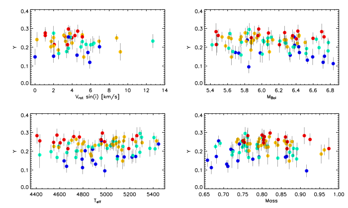
Figure 8: Helium content deduced from the isochrones as function of $V_{rot}\sin(i)$ (available for 45 K dwarfs), $M_{Bol}$, $T_{eff}$ and Mass for all our 86 K dwarfs. Stars are divided in the same metallicity bins and colours as in Figure 3. No obvious dependence appears and low $Y$ values are practically present throughout the entire range of parameters covered by our stars.

The absence of any obvious trend is a posteriori confirmation of the adequacy of the adopted evolutionary cut $M_{Bol}\geq 5.4$. Figure 8 shows that most of our stars have masses (deduced from the isochrones) below $0.85M_{\odot}$ at low $Z$. Studies of globular clusters in the Milky Way also confirm that metal-poor stars below $0.80-0.85M_{\odot}$ have not yet reached the turn-off, the exact value depending on the age and the underlying details of the isochrones used to fit a globular cluster (e.g. Chaboyer et al. 2001; Morel & Baglin 1999). For higher metallicity the turn-off mass is also higher, making evolutionary effects even less likely in such stars in our sample.

5.3 Shortcomings in stellar models

Despite the steady improvement in modeling stellar structure and evolution, there are still shortcomings in the theory that require the introduction of adjustable parameters, typically calibrated on the Sun.

Our model is calibrated on the Sun, for an assumed $Z_{\odot}=0.017$, by adjusting the helium content and the mixing-length in order to match its present age, radius and luminosity (Section 3.2). As we already pointed out, the $Y_{\odot}$ value must be intended as the zero-point of our calibrated model and not as the absolute value of the solar helium content. Helioseismology does in fact return a lower helium content but including diffusion in the model helps to reduce such a difference (see Section 5.3.2). The difference between the present helium value derived from seismology and the initial value obtained from the calibration provides a constraint on the input physics of the model.

The fact that we are working with stars that are only slightly cooler and fainter than the Sun should ensure that we are studying a region of the HR diagram where models, at least for metallicities around the solar one, are well calibrated. Our solar isochrone is in fact in outstanding agreement with a sample of solar metallicity stars (Figure 1).

5.3.1 Mixing-length

The universality of the mixing-length value is an open question. The analysis of binaries in the Hyades has recently lead Lebreton et al. (2001) and Yildiz et al. (2006) to conclude that the mixing-length increases with stellar mass. Similar conclusions were also drawn by Morel et al. (2000a) and Lastennet et al. (2003) based on the study of the binary systems $\iota$ Peg and UV Piscium, respectively. These results are opposite to the theoretical expectation from hydrodynamical simulations of convection (Ludwig, Freytag & Steffen 1999; Trampedach et al. 1999). Detailed calibration of stellar models on the $\alpha$ Cen system have returned discordant conclusions about the universality of the mixing length parameter (e.g. Noels et al. 1991; Edmonds et al. 1992; Neuforge 1993; Fernandes & Neuforge 1995; Morel et al. 2000b; Guenther & Demarque 2000). The latest model calibrations on the $\alpha$ Cen system making use of seismic constraints favor a mixing-length that increases going to lower mass (Eggenberger et al. 2004; Miglio & Montalbán 2005) and therefore in agreement with the theoretical expectations. The discordant conclusions drawn from all these studies probably reflect the many observational uncertainties (order of magnitudes larger than for the Sun) in the input parameters of the models. These results suggest that at this stage a clear relation between mass and mixing-length is premature, either because uncertainties in the input parameters can overshadow shortcomings in the mixing-length theory itself, or because a dispersion of mixing-length at a given mass or even a time dependence of the mixing-length (Yildiz 2007) could well be possible. Therefore, assuming the solar mixing length is currently the safest choice. Systematic trends in mixing length are anyways overwhelmed by observational uncertainties.

As regards the dependence on the metallicity, the fact that all globular clusters can be fit with the same value for the mixing length parameter supports the assumption that it does not depend on $Z$, although such a conclusion is obtained studying giant branch stars only (e.g. Jimenez et al. 1996; Palmieri et al. 2002; Ferraro et al. 2006). Concerning the particular region of the HR diagram we are going to investigate, models computed with the solar mixing-length reproduce the slope of the main sequence of young open clusters quite well (VandenBerg & Bridges 1984; Perryman et al. 1998) and of field stars (Lebreton et al. 1999) observed by Hipparcos. In addition, the study of lower main sequence visual binary systems with known masses and metallicity returns a mixing-length unique and equal to the solar one for a wide range of ages and metallicities $\textrm{[Fe/H]}_{\odot}\pm 0.3$ dex (Fernandes et al. 1998).

Nonetheless, a decrease of the mixing length at low $Z$ would be particularly interesting since it would produce a less massive convection zone for a given stellar mass, thus making isochrones cooler. For metal poor stars this effect could partly alleviate our “low helium” problem. We have tested the effect of setting the mixing length $\alpha_{\rm MLT}=1.00$ and the difference with respect to the adopted solar one ($\alpha_{\rm MLT}=1.68$) is shown in Figure 9 for a moderately helium deficient and metal poor isochrone. As a result, a large change in the mixing length is indeed able to shift the isochrone to cooler temperatures, thus improving the agreement with the data.

Figure 9: Effect of changing the mixing length $\alpha_{\rm MLT}$ in a metal poor isochrone (age 5 Gyr, although the age does not play any role). The dotted horizontal line is the adopted cut in $M_{Bol}$ for our sample of stars (see Section 2). Overplotted are also our dwarfs with $Z\sim 0.001$.

This result can be regarded as an indication of a metallicity dependence of the mixing-length for the lower main sequence, as already suggested by Chieffi, Straniero & Salaris (1995). Whether such a large change in $\alpha_{\rm MLT}$ is justified on other evidence or physical grounds remains to be seen. In this work we rather test to which extent the most recent low mass stellar models can be used ipse facto to study a large stellar sample in the Solar Neighbourhood. The range in which models can be safely used is discussed in Section 6.

5.3.2 Diffusion

Atomic diffusion (sometimes called microscopic or elemental diffusion) is a basic transport mechanism which is usually neglected in standard stellar models. It is driven by pressure, temperature and composition gradients. Gravity and temperature gradients tend to concentrate the heavier elements toward the center of the star, while concentration gradients oppose to the above processes (e.g. Salaris, Groenewegen & Weiss 2000). To be efficient, the medium has to be quiet enough, so that large scale motion cannot prevent the settling (e.g. Morel & Baglin 1999; Chaboyer et al. 2001). Diffusion acts very slowly, with time scales of the order of $10^{9}$ years so that the only evolutionary phase where diffusion is efficient is during the Main Sequence, in particular for metal poor (Population II) stars because of their small convective envelopes. For the Sun, the insertion of helium and heavy element diffusion in the models has significantly improved the agreement between theory and observations (e.g. Christensen–Dalsgaard, Proffitt & Thompson 1993; Guenther & Demarque 1997; Bahcall at al. 1997; Basu, Pinsonneault & Bahcall 2000). Only in the region immediately below the the convective envelope theoretical models deviate significantly from the seismic Sun, indicating that diffusion might not operate exactly in the way calculated or pointing to some neglected additional physical process partially counteracting diffusion (Brun et al. 1999).

Due to diffusion the stellar surface metallicity and helium content progressively decrease during the main sequence phase as these elements sink below the boundary of the convective envelope. In the deep interior, the sinking of helium towards the core leads to a faster nuclear aging, thus reducing the main sequence lifetime with consequences for age determinations of Globular Clusters (Chaboyer et al. 1992; Castellani et al. 1997). In the envelope, diffusion leads to a depletion of the heavy elements and helium thus producing a decrease of the mean molecular weight. Metal diffusion decreases the opacity in the envelope and increase the central CNO abundance: the dominant effects are the decrease of the mean molecular weights in the envelope and its increase in the core which increases the model radius and hence decreases the effective temperature. The net effect on the evolutionary tracks, for a given initial chemical composition, is to have a main sequence cooler. This effect reaches its maximum at the turn-off stage, after which a large part of the metals and helium diffused toward the center are dredged back into the convective envelope of giant branch stars, thus restoring the surface $Z$ and $Y$ to a value almost as high as for evolution without diffusion (e.g. Salaris et al. 2000).

Diffusion is clearly a major candidate in helping to solve the puzzling low helium abundances of Section 4, since it yields a cooler main sequence, thus operating in the required sense. Besides the effect on the stellar models themselves, diffusion affects the measured surface metallicities with respect to the true (original) ones of the stars, altering conclusions about $Y(Z)$ (see below). In their pioneering work, Lebreton et al. (1999) found that main sequence models (for standard values of helium enhancement) were hotter than Hipparcos subdwarfs in the metallicity range $-1\leq\textrm{[Fe/H]}\leq-0.3$. Since decreasing the helium abundance to resolve the conflict would have required values well below the primordial one (in accordance to what we have obtained in Section 3.3 and 4), Lebreton et al. (1999) advocated two processes that could help in solving the discrepancy : i) diffusion of helium and heavier elements in stellar models and ii) increase of the measured metallicity in metal poor objects due to usually neglected NLTE effects. Correcting isochrones for both effects they were partly able to solve the discrepancy (see also Morel & Baglin 1999), but their number of metal poor and faint stars was rather modest. Here we test the same corrections on many more stars.

We focus only on the effects of diffusion, leaving the discussion of observational uncertainties (among which NLTE effects) to Section 5.4. The works of Morel & Baglin (1999) and Salaris et al. (2000) specifically tackle the effects of helium and heavy elements diffusion in field stars. Both works assume a full efficiency of the diffusion so that their results can be regarded as an upper limit on its effects.

From the observational point of view, diffusion decreases the surface metallicity –provided that it is fully efficient and no other processes counteract it– so that a star presently observed with a given [Fe/H] has started its evolution with a larger metallicity $\textrm{[Fe/H]}_{0}$. As we discuss later such a difference is of order $0.1$ dex, although sometimes higher differences have been claimed. Such a shift in metallicity has negligible effects on the fundamental parameters of $T_{eff}$ and $M_{Bol}$ determined for our stars with the IRFM (figure 11 in Casagrande et al. 2006), yet it would imply that our fits in Figures 4–6 are performed with too low Z isochrones, thus needing low $Y$ values to compensate for the hot isochrone temperatures.

A proper comparison between diffusive and non-diffusive isochrones therefore must take into account also that diffusive isochrones must start their evolution with a higher metallicity so that at a chosen age their surface metallicity (which decreases with time) matches that of non-diffusive isochrones. Following the notation of Morel & Baglin (1999) we call isochrones that account for both effects (diffusion and correction of the surface metallicities) “diffusive calibrated isochrones”. Diffusion clearly introduces an age dependence regardless of the fact that stars are still on their ZAMS. As a general rule, depletion increases with increasing age since diffusion has more time to work. Differences between non-diffusive and diffusive calibrated isochrones are given by Salaris et al. (2000) for various metallicities, ages and luminosities. The calibrated diffusive isochrones are cooler by a few tens up to $100-150$ K, depending on mass and age (see figure 2 in Salaris et al. 2000). However, for the lower main sequence the effect of diffusion becomes increasingly less significant (their table 1). At the lowest masses and faintest luminosities covered in this study the effect of diffusion is at most $30-40$ K in $T_{eff}$. The reason for such negligible changes is that in the low mass regime, stars have large convective zones which inhibit diffusion. Figure 8 clearly shows that low values of helium are also found for objects with masses below $0.7M_{\odot}$, thus suggesting that diffusion is not the only relevant ingredient to solving our helium discrepancy. Similar results to those of Salaris et al. (2000) were also found by Morel & Baglin (1999) who give a large set of corrections between non diffusive and diffusive calibrated isochrones. Their corrections are provided for 10 Gyr isochrones in the metallicity range $0.0006\leq Z\leq 0.006$ and masses between $0.6-0.85M_{\odot}$. Their age is chosen in order to maximize the effect of diffusion. At this age, masses above $0.85M_{\odot}$ start to evolve off the main sequence; for masses below $0.6M_{\odot}$ the effect of diffusion is negligible. We apply these corrections to our isochrones and we consider only masses below $0.85M_{\odot}$. We linearly interpolate such corrections between contiguous values of $M_{bol}$, $T_{eff}$ and $Z$ and apply them to all our sub-solar metallicities isochrones. In the range $0.006<Z<0.017$ we have extrapolated them. Notice that the corrections in Morel & Baglin (1999) are given for isochrones with standard values of $Y(Z)$ whereas here we apply them to isochrones with a large range of $Y(Z)$. However, the main effect of diffusion is to alter to surface $Z$ and that does not depend on $Y$.

The results of computing the helium abundances for our stars with the corrected isochrones are shown in Figure 10. Diffusion clearly helps in increasing the inferred helium fractions and its effect –as expected– becomes more important going to lower metallicities. However extremely low helium abundances at the lowest $Z$’s are still found.

Figure 10: First panel: $Y$ versus $Z$ plot when the effects of diffusion are included (squares) or not(circles) in the computation. The vertical dotted lines are the metallicity range for which Morel & Baglin (1999) give corrections. We have extrapolated such corrections up to the solar metallicity $Z=0.017$. For higher metallicities only circles are shown. Second and third panel: dependence of $Y$ with Mass and $M_{Bol}$. Error bars are not shown for clarity purpose, but are of same magnitude as in Figure 7 and 8.

The fact that low helium abundances are now preferentially found among the fainter and less massive stars reflects the fact that –as anticipated– corrections due to diffusion become less and less important descending along the main sequence. Still, disturbingly low values of $Y\sim 0.2$ remain for any mass and luminosity, although more orthodox values are within the error bars.

Until now we have estimated the effect of diffusion in the case of full efficiency of this process. However there are many observational evidences suggesting diffusion is less effective.

Diffusion is expected to be more important in metal poor stars, where the mass of the convective envelope is smaller (e.g. Chaboyer et al. 2001); however, whether it effectively occurs and how efficiently is still matter of debate, and especially at low metallicities. Observations of the narrow Spite Li–plateau in metal-poor stars (Spite & Spite 1982; Thorburn 1994; Ryan, Norris & Beers 1999; Asplund et al. 2006; Bonifacio et al. 2007) suggest that diffusion is inhibited near the surface of these objects (e.g. Deliyannis & Demarque 1991; Chaboyer & Demarque 1994; Ryan et al. 1996) although Salaris & Weiss (2001) pointed out that after carefully accounting for uncertainties and biases in observations, models with diffusion are still in agreement with observations. More recently Richard et al. (2005) invoked a ‘turbulent diffusion’ which would limit diffusion without mixing Li. If Li does not allow firm conclusions, [Fe/H] is a much more robust diagnostic (e.g. Chaboyer et al. 2001). The absence of any variation in [Fe/H] between giant branch and turn-off stars found by Gratton et al. (2001) for two globular clusters (NGC6397 with [Fe/H] $=-2.03$ and NGC6752 with [Fe/H] $=-1.42$) is a very strong evidence that sedimentation cannot act freely in all stars. Regarding field stars, diffusion must affect the measured [Fe/H] only marginally, for otherwise high-velocity giants in the Hipparcos catalogue would have on average metallicity larger by a factor of two than their turn-off or main sequence counterparts, a feature which has not been observed (D’Antona et al. 2005b).

Diffusion changes the slope of the main sequence, rendering it steeper as one goes to higher luminosities (Morel & Baglin 1999; Salaris et al. 2000) and also produces a distortion in the mass-luminosity relation (Morel & Baglin 1999) so that extremely accurate data could, in principle, detect it. Interestingly, within the present day accuracy, our results agree with mass-luminosity relations (see Section 7). Since the efficiency of diffusion changes with metallicity –if diffusion actually occurs– a much larger sample of disk stars than those used in this study (so that the time on which diffusion has been acting is on average the same and equal to the mean age of the disk) would probably make possible to detected a change in the slope of the location of dwarfs with metallicity say, solar and a third of the solar value.

From the point of view of theoretical modeling, the effect of heavy element diffusion in metal poor stars is still controversial (e.g. D’Antona et al. 2005b; Gratton, Sneden & Carretta 2004) as theoretical results also differ according to the formalism employed to describe it. Models that assume complete ionization (and then negligible effects of radiation pressure) predict depletion for all elements heavier than H (e.g. Straniero, Chieffi & Limongi 1997; Chaboyer et al. 2001). However, accounting for partial ionization and radiation pressure shows that whereas some elements like He and Li are expected to be depleted, others (like Fe) are expected to be significantly enhanced for stars with $T_{eff}>6000$ K and only moderately underabundant ($\sim 0.1$ dex or less) below this temperature (Richard et al. 2002). Chaboyer et al. (2001) found that models with full diffusion differ by more than $2\sigma$ from the observations of Gratton et al. (2001), thus concluding that heavy-element diffusion does not occur in the surface layers of metal-poor stars and that isochrones including the full effects of diffusion should not be used for comparison with observational data. Although it is not yet clear which mechanism can counteract diffusion in the surface layers –mass loss (Vauclair & Charbonnel 1995), mixing induced by rotation (e.g. Vauclair 1988; Pinsonneault et al. 1992, 1999, 2002) and radiative diffusion (Morel & Thévenin 2002) have been proposed among others– Chaboyer et al. (2001) found that the temperatures of models in which diffusion is (admittedly ad hoc) inhibited near the surface (but not in the deep interior) of metal poor stars are similar to the temperatures of models evolved without diffusion. Also Richard et al. (2002) concluded that at least in $0.8M_{\odot}$ stars, it is a better approximation not to let Fe diffuse than to calculate its gravitational settling without including the effect of radiative acceleration.

In summary, all models predict the effect of diffusion to increase with decreasing metallicity, since at lower $Z$ the main sequence shifts to hotter temperatures, for which convective layers are smaller. At the same time, Lithium (to some extent) and the most accurate [Fe/H] measurements in globular clusters (Gratton et al. 2001) pose an upper limit to the effect of diffusion that even for the most metal poor stars in our sample is expected (if any) to be negligible or within our error bars. The results shown in Figure 10 assume a fully efficient diffusion that is improbable and still do not solve completely the problem of our low helium abundances.

5.4 NLTE effects and adopted temperature and luminosity scale

As previously noted, Lebreton et al. (1999) were partly able to resolve the low helium abundance problem by using the cumulated effect of diffusion and NLTE departures in metallicity measurements. According to Thévenin & Idiart (1999) NLTE corrections are negligible for stars with solar metallicity but for $\textrm{[Fe/H]}\sim-1.0$ the measured metallicity should be increased of order 0.15 dex (the larger corrections being for hotter –$T_{eff}>6000$ K– stars that however we do not have in our sample). Such a difference, although significant, is roughly of the same order of present day uncertainties in abundance determinations. Besides, the relatively large differences claimed by Thévenin & Idiart (1999) have not been confirmed by other subsequent studies. Gratton et al. (1999) found negligible departures from LTE in dwarf stars of any $T_{eff}$ concluding that LTE abundance analysis of metal poor dwarfs are validated, an important support to the current views on galactic chemical evolution. Gratton et al. (1999) also analyzed NLTE effects on species other than Fe and again they did not find any significant departures in the case of cool dwarfs. Similar conclusions were drawn by Fulbright (2000) and Allende Prieto et al. (1999) pointed out that NLTE starts to show up primarily at $\textrm{[Fe/H]}<-1.0$ (i.e $Z\lesssim 0.003$ whereas our low Y values are already found at higher metallicities). Thorough calculations accounting for NLTE effects have been carried out by Gehren et al. (2001a, 2001b), Korn, Shi & Gehren (2003) who found negligible corrections for the Sun and up to 0.06 dex in the case of halo stars. The effects of departures from LTE in abundance determinations of various elements are widely discussed in Asplund (2005). Summarizing, in the case of Iron lines a clear consensus about NLTE effects is still far from reach, but it seems reasonable to assume that corrections of order 0.10 dex are expected in stars with low metallicities and/or $\log g$.

The metallicities we use come from various sources (Casagrande et al. 2006), so that this might account for part of the scatter in the data. However, the overall trend is clear and therefore does not depend on the specific metallicity scale adopted. Besides, in the colour-colour planes (expecially in the $B-V$ colour index which is very sensitive to metallicity) there is a very good agreement between our sample of stars and the homogeneous metallicity scale of model atmospheres (Casagrande et al. 2006). We have already mentioned that our work is differential with respect to the Sun and therefore we expect our results to be unaffected by the new solar abundances obtained when 3D model atmospheres are adopted, provided that similar updates pertain also to the lower main sequence stars. However, large libraries of 3D model atmosphere for analyzing stellar spectra are not yet available. Therefore, we can not exclude a priori that there are no systematic biases in the models with $Z$.

We also test whether the low helium abundances depend on the adopted temperature and luminosity scale. Our empirical IRFM temperature (and luminosity) scale is in agreement with spectroscopic measurements and $\sim 100$ K hotter than other IRFM temperature scale (see Casagrande et al. 2006 for a detailed discussion); it closely recovers the temperatures of a set of solar analogs and indeed the theoretical solar isochrone is in outstanding agreement with the data (Figure 1). Cooler temperature scales clearly tend to increase the disagreement with respect to theoretical isochrones, although when studying the HR diagram it is the combined effect of temperature and luminosity scales which is important. In this respect, the IRFM is one of the few methods that returns a fully consistent temperature and luminosity scale.

If we adopt the IRFM scale of Ramírez & Meléndez (2005) by decreasing our effective temperatures by 100 K and luminosities by 1.4% (Casagrande et al. 2006) the problem of low helium abundances becomes still worse. The shape of the $Y$ vs. $Z$ plot is the same (reflecting the offset in the absolute calibration adopted, Casagrande et al. 2006) but the helium content is on average lower by $\sim 0.04$ so that already at solar metallicity the bulk of stars has a helium content lower than our solar calibrated model.

6 The binary test

To date, the most stringent tests of the theory of stellar structure and evolution have been carried out for the Sun. Its mass, luminosity and radius are known to better than 1 part in $10^{3}$ and its age to better than few percent (e.g. Guenther & Demarque 2000; Bahcall, Serenelli & Basu 2006). Its chemical abundance, which sets the zero point of metallicity measurements in other stars, is currently under profound discussion (Asplund et al. 2005) however, as we have already mentioned, this change should not affect dramatically our study since our work is differential with respect to the Sun. The Sun is therefore the natural benchmark in understanding and setting models of stellar structure and evolution. We have already checked the solar isochrone to be in excellent agreement with our solar metallicity stars (Figure 1).

In the case of stars other than the Sun, radii and luminosities are known with much less accuracy although interferometry is expected to be a major breakthrough in the next few years. For the moment, masses can be empirically determined only in the case of systems in binaries. For visual binaries with well-measured parallaxes, the uncertainty in mass determination is rarely less than 1%, a value that sets the accuracy required to provide important constraints on models of stellar structure and evolution (e.g. Andersen 1991). In addition to the mass, the measured colours and metallicities are another source of errors.

As we have already discussed in Section 4 such limitations preclude the accurate calibration of stellar models on binary stars. Our model is calibrated on the Sun but the comparison with a statistically congruous number of binaries can indeed provide important constraints on it. Here we use various double stars with accurately measured masses, metallicities and colour indices for at least one of the components. They are all nearby, so that no reddening corrections are needed. Colours and metallicities are used to derive $T_{eff}$ and $M_{Bol}$ consistently with our IRFM scale. The mean metallicity from various recent measurements is used so as to reduce the uncertainty in this observable. The same procedure as described in Section 4 is then applied to deduce the mass and the helium content of these binaries. Although the broadening (and so the helium content) of the lower main sequence is independent of assumptions about stellar age, masses are not, as we have quantified in Section 4. Here we are interested in testing to what extent our choice of using 5 Gyr old isochrones is on average able to recover the masses of lower main sequence dwarfs. Though with a large scatter such age should be in fact representative of the Solar Neighbourhood (Reid et al. 2007), also considering there is no clear consensus on the tightness of the age–metallicity relation (e.g. Feltzing et al. 2001), so that older isochrones are not necessarily the most appropriate for metal poor stars. The masses deduced from the isochrones are compared to those measured empirically: if the masses are recovered with an accuracy of few percent the corresponding helium content of the stars –which is practically age independent– is also validated (Figure 6).

Note that to have a congruous number of stars, we have slightly relaxed our cutoff on $M_{Bol}$. Possible evolutionary effects have therefore been taken into account for the brightest stars, but if not otherwise specified the age adopted for the isochrones is fixed to 5 Gyr. We also mention that all these stars belong to non-interacting binary systems so they are representative of single stars.

6.1 $\alpha$ Cen B

Among stars other than the Sun, the $\alpha$ Cen system is probably the most used test-bed for checking stellar models (see also discussion in Section 5.3.1). Its secondary component (HD 128621) is a K dwarf and it has been a privileged target for asteroseismic (e.g. Thévenin et al. 2002; Kjeldsen et al. 2005) and interferometric (Kervella et al. 2004; Bigot et al. 2006) studies. Since it is in a well separated binary this K dwarf is part of our original sample of Section 2, but here we analyze the results in more detail. Using positions and radial velocities, its mass has been estimated to great accuracy ($M=0.934\pm 0.0061\,M_{\odot}$) and completely independently of theoretical considerations of stellar structure and evolution (Pourbaix et al. 2002). For this star there are various independent and accurate metallicity measurements (Valenti & Fischer 2005; Santos et al. 2005; Allende Prieto et al. 2004; Feltzing & Gonzalez 2001) with a mean value $\textrm{[Fe/H]}=0.23\pm 0.03$ dex and solar scaled abundances. Accurate $BV(RI)_{C}$ colours (Table 3) are available from Bessell (1990) from which $T_{eff}$ and $M_{Bol}$ are computed as described in Section 2. We obtain a mass of $0.925\pm 0.035M_{\odot}$ in excellent agreement with that measured empirically. The corresponding helium content is found to be $0.262\pm 0.022$ and therefore equal to the solar one within errors, although the star is more metal rich.

6.2 vB22

As summarized by Lebreton et al. (2001), the Hyades cluster has five binaries whose components have measured masses. Of these systems only the eclipsing binary HD 27130 (vB22) has masses with small enough uncertainty to place significant constraints on theoretical models, as studied by Pinsonneault et al. (2003). $BV(RI)_{C}$ magnitudes and colours of both components are available from Schiller & Milone (1987) and are listed in Table 3. Again, $T_{eff}$ and $M_{Bol}$ are derived according to the procedure described in Section 2. Though metallicity measurements for an eclipsing binary are quite uncertain, we exploit the fact that the metallicity of such a system must be the same of other cluster members. For the Hyades, Paulson, Sneden & Cochran (2003) have conducted a detailed spectroscopic analysis from which a mean metallicity $\textrm{[Fe/H]}=+0.13\pm 0.04$ dex and solar scaled abundances have been derived. High-precision distance estimates are available from Hipparcos ($\omega=21.40\pm 1.24$) and from a kinematic parallax (de Bruijne et al. 2001, $\omega=21.16\pm 0.38$ mas). These are all in excellent agreement and we assume de Bruijne et al. (2001) measurement in the following.

Empirical masses are available from Torres & Ribas (2002). For the mass and bolometric magnitude of the primary, age effects become relevant and, rather than our standard reference 5 Gyr isochrones, we consider isochrones of 500 Myr (1 Gyr), consistent with the age of the cluster (Perryman et al. 1998). The estimated mass is 1.100 (1.088) $M_{\odot}$ ($1\sigma$ more massive than the empirical value) and the corresponding helium content $Y\sim 0.22$. Optimizing on the mass formally returns an age of 2.48 Gyr and $Y\sim 0.23$. Evidently age effects are important here, but in any case, the helium content of the system is significantly below solar. For the secondary, as expected, the helium content is independent of the age chosen for the isochrones. The difference in the use of 500 Myr and 5 Gyr isochrones is less than 0.02 in mass and 0.004 in helium abundance, i.e. smaller than the uncertainty of the results. Using 5 Gyr isochrones, the mass we recover for the secondary is in very good agreement with the empirical one, with a helium content significantly lower than the solar one. Though depending also on the exact metallicity of the binary (we have assumed the average value of the cluster, but a slight scatter among its stars is possible), our result provide a further, strong evidence that the Hyades are underabundant in helium for their metallicity (Perryman et al. 1998; Lebreton et al. 2001; Pinsonneault et al. 2003).

6.3 $70$ Oph

$70$ Oph (HD 165341) is one of our nearest neighbours and is among the first discovered binary stars. Gliese & Jahreiß (1991) classify it as a primary of spectral type K0 V and a secondary of type K5 V. Recent abundance analysis for the primary companion are available from Luck & Heiter (2006), Mishenina et al. (2004), Allende Prieto et al. (2004). We adopt the mean value $\textrm{[Fe/H]}=-0.02\pm 0.08$ dex and $\textrm{[}\alpha\textrm{/Fe]}=0.06\pm 0.11$ dex. Tycho $B_{T}$ and $V_{T}$ magnitudes for both components are available from Fabricius & Makarov (2000) which we convert to the Johnson-Cousins system by interpolating the transformation coefficients given in table 2 of Bessell (2000). Additional photometry is available from Gliese & Jahreiß : $V$ magnitudes agree with the transformed Fabricius & Makarov (2000) ones within $0.01$ mag, whereas the $B-V$ index of Gliese are slightly ($0.02-0.04$ mag) redder. $(R-I)_{K}$ from Gliese & Jahreiß has been converted to the Cousins system with the transformation given in Bessell (1995). For consistency with the choice made for most of the binaries we use only magnitudes and colours from Gliese & Jahreiß. Averaging with the $B$ and $V$ magnitudes from Fabricius & Makarov (2000) hardly changes the results : the large uncertainty in $T_{eff}$ for the primary component remains the same and the changes in the helium content and masses of both components are smaller than their final errors. We use the Hipparcos parallax and errors as corrected by Söderhjelm (1999) ($\omega=195.70\pm 0.90$ mas) for binarity effects. Masses for the primary and the secondary are available from Henry & McCarthy (1993) ($M=0.856\pm 0.056\,M_{\odot}$ and $M=0.713\pm 0.029\,M_{\odot}$, the secondary as recomputed with an improved parallax by Delfosse et al. 2000) and from Fernandes et al. (1998) ($M=0.89\pm 0.04\,M_{\odot}$ and $M=0.71\pm 0.04\,M_{\odot}$) that we assume in the following. Based on asteroseismic considerations Carrier & Eggenberger (2006) also derived a mass of $0.87\,M_{\odot}$ for the primary component. The masses we derive are in good agreement with the empirical ones although the large uncertainty in $T_{eff}$ of the primary returns considerably large error bars. The helium content is equal to the solar one within the errors, consistently with the expectation given the solar metallicity. A solar helium abundance was also obtained by Fernandes et al. (1998).

6.4 HD 195987

Combining spectroscopic and interferometric observations for this double-lined binary system, Torres et al. (2002) derived masses with a relative accuracy of a few percent. They also determined the metallicity ([Fe/H]$=-0.5$, [$\alpha$/Fe]$=+0.4$ and uncertainty $\sim 0.2$ dex), orbital parallax ($\omega=46.08\pm 0.27$ mas in rough agreement with the Hipparcos value, but with smaller formal error) and $V,H,K$ magnitudes for both components. Their infrared magnitudes are in the CIT system and we convert them into the 2MASS by using the Carpenter (2001) transformations. We then use our effective temperature and bolometric luminosity calibrations and the procedure described in Section 4 to deduce the mass and helium content of both components. The mass of the primary is higher by $3\sigma$ but that of the secondary is in good agreement with the empirical value. Both components are fitted with similar (and well below primordial) helium content. Ascribing the mass discrepancies to temperature effects, an increase of 70 K in the $T_{eff}$ of the secondary (or more properly a corresponding decrease in the effective temperature of the isochrones) would return a mass ($0.666M_{\odot}$) in excellent agreement with the empirical one, but the helium content would be still very low ($Y=0.180$). For the primary the temperature should be increased by 300 K in order to obtain a mass ($0.842M_{\odot}$) in agreement with the empirical one. In this case the helium content would be $Y=0.269$, higher than that of our solar calibrated model. However, the primary is very luminous given its mass, so that it could be a slightly evolved stars and therefore 5 Gyr isochrones could not be the most appropriate choice. If 10 Gyr old isochrones are used, masses are decreased so that the primary is off by $2\sigma$ and both components are again fitted with similar helium content.

6.5 $\xi$ Boo

$\xi$ Boo (HD 131156) consists of a primary of spectral type G8 V and a secondary K4 V (Gliese & Jahreiß 1991). The primary is known to be very active, with irregular fluctuations of activity (e.g. Petit et al. 2005 and references therein) and a high chromospheric emission (Baliunas et al. 1995) being classified as flare star in SIMBAD and variable in Hipparcos. These data suggest a young age that also agrees with conclusions from evolutionary models (Fernandes at al. 1998). Recent abundance analyses for the primary component are available from Luck & Heiter (2006), Valenti & Fischer (2005), Allende Prieto et al. (2004), Fuhrmann (2004). We adopt the resulting mean value $\textrm{[Fe/H]}=-0.15\pm 0.09$ dex and $\textrm{[}\alpha\textrm{/Fe]}=-0.06\pm 0.15$ dex. $V$ magnitudes, $B-V$ and $(R-I)_{K}$ indices of both components are available from Gliese & Jahreiß (1991). We convert $(R-I)_{K}$ into Cousins system by means of the Bessell (1995) transformations. Improved Hipparcos parallaxes are available from Söderhjelm (1999) and empirical masses from Fernandes et al. (1998).

The results are certainly interesting : the primary is more massive than the empirical value, whereas the secondary is $2\sigma$ less massive. Also, the helium content between the two component differs by $1\sigma$, whereas all the other binaries in this study have identical helium abundances within the errors. To reach a closer agreement with the empirical masses, that of the primary should be decreased (implying a higher helium abundance, see Figure 6) whereas that of the secondary should be increased (thus lowering its helium content). Of course, the photometry could be adversely affected by the young system age and be the simple explanation for these puzzling results. Torres et al. (2006) found chromospheric activity as a likely cause of the discrepancy between models and observations in the case of another star (HD 235444). We have decided to discard this binary from our basic sample of stars with empirical masses.

One might still wonder whether variability can occur among some of the stars in Section 2 and to what extent this might be behind our anomalous helium abundances. Extensive surveys by Einstein and ROSAT and Chandra X-ray satellites have shown that late-type main sequence stars are surrounded by coronae analogous to the more easily observed solar corona (e.g. Schmitt & Liefke 2004; Wood & Linsky 2006). Flares, spots, coronal mass ejections, prominences are, of course, not exclusive to our Sun. For our sample of stars we have used the $\Delta\mu$ method to remove unresolved binaries (whose tidal interaction could trigger activity, e.g. Torres et al. 2006) and the same sample is also free from variable stars to a high accuracy level (Casagrande et al. 2006). Therefore, any intrinsic level of activity in the sample of Section 2 is below our observational uncertainties and is unlikely to be causing our helium discrepancies. Furthermore, to explain the low helium abundances, variability should practically be limited to the metal poor stars, whereas variability is known to occur at all metallicities.

6.6 $\eta$ Cas B

$\eta$ Cas (HD 4614) is a nearby visual binary at a distance $\sim 6$ pc. According to Gliese & Jahreiß (1991) it consists of a primary of spectral type G3 V and a secondary K7 V. $\eta$ Cas A is known to be over-luminous with respect to the mass-luminosity relation, thus suggesting that it has begun to evolve off the main sequence (Fernandes et al. 1998). In what follows we focus on the secondary, $\eta$ Cas B. Abundance analyses for cool dwarfs are still challenging (e.g. Bonfils et al. 2005), however the metallicity of the primary is well determined. We have taken five independent metallicity measurements (most of which include $\alpha$-elements) from Luck & Heiter (2006), Valenti & Fischer (2005), Bonfils et al. (2005), Mishenina et al. (2004), Allende Prieto et al. (2004). All these measurements show good agreement and we adopt a mean value of $\textrm{[Fe/H]}=-0.31\pm 0.07$ dex and $\textrm{[}\alpha\textrm{/Fe]}=0.10\pm 0.03$ dex. Visual magnitude, $(B-V)$ and $(R-I)_{K}$ colours for the secondary are also available from Gliese & Jahreiß (1991). $(R-I)_{K}$ is in the Kron system and it has been converted to the Cousins system with the transformation given in Bessell (1995). Both colours are slightly redder than the applicability range of our temperature and bolometric luminosity calibrations, consistently so with the late spectral type of this star. However the mean loci of the calibrations in Casagrande et al. (2006) (see their figure 13 and 18) show well defined trends so that the extrapolation to stars $\sim 100$ K cooler than the applicability range is still quite reasonable. The parallax of the primary is available from Hipparcos and the mass of the secondary from Fernandes et al. (1998). Notice that both the spectral type and the mass of this star are slightly lower than that of our sample stars in Section 2. The result for this moderately metal deficient star is particularly interesting, since it does yield a low helium abundance (but in agreement with the bulk of stars with the same metallicity in Figure 7) while its derived isochrone mass is lower than the empirical value. At this metallicity NLTE effects in the derived metallicities should be very small if any, as well as the effect of diffusion that are negligible at $0.6M_{\odot}$. Also, from Figure 6 an increase of the mass at fixed metallicity would require an even lower helium abundance.

As noted above, Fernandes et al. (1998) calibrated stellar models to this binary, obtaining a helium content ($Y=0.25$) higher than that found here. However, considering the difference in the respective solar reference value (their solar model has $Y_{\odot}=0.28$) our result is within $1\sigma$ with theirs.

6.7 $85$ Peg A

85 Peg (HD 224930) is a well studied, metal poor, visual and single-lined spectroscopic binary. Its small angular separation and the marked magnitude difference between the components ($\Delta m_{V}=3.08\pm 0.29$ mag, ten Brummelaar et al. 2000), makes it a difficult target both for visual and spectroscopic observations. The given $\Delta m_{V}$ implies a magnitude correction of $0.06$ mag for the primary that increases going to longer wavelength ($0.12$ mag in $I$, see equation 3). The contribution of the secondary thus must be properly removed. The total mass of the system is well constrained from visual orbital elements and Kepler’s third law (e.g. Griffin 2004; Fernandes et al. 2002) however the masses of the individual components are much more uncertain.

For the primary 85 Peg A, we adopt a mass of $0.84\pm 0.08M_{\odot}$, as obtained by Fernandes et al. (2002) and in near agreement with D’Antona et al. (2005b) who, based on model predictions, estimated the mass to be in the range 0.75 to 0.82 $M_{\odot}$. For many years investigators have claimed that 85 Peg B, the fainter companion, is more massive than 85 Peg A, the brighter one (e.g. Hall 1948; Underhill 1963; Heintz 1993) and this abnormal situation could be explained if 85 Peg B is an undetected binary, as already suggested by Hall (1948). Indeed, this seems to be the case, as the same conclusions can be drawn when the position of both components in the HR diagram is compared with theoretical expectations (Fernandes et al. 2002; D’Antona et al. 2005b). In what follows we only consider the primary component. We use the Hipparcos parallax and errors as corrected by Söderhjelm (1999) ($\omega=82.50\pm 0.80$ mas) for binarity effects. For the metallicity we adopt the mean value obtained from six recent independent determinations (Luck & Heiter 2006; Mishenina et al. 2004; Allende Prieto et al. 2004; Fuhrmann 2004; Gratton et al. 2003; Fulbright 2000). All these measurements show good agreement with an average $\textrm{[Fe/H]}=-0.90\pm 0.06$ dex and $\textrm{[}\alpha\textrm{/Fe]}=+0.40\pm 0.04$ dex. Spectroscopic determinations return temperatures ranging from $\sim 5300$ K (Fulbright 2000) to $\sim 5600$ K (Fuhrmann 2004), the latter being in close agreement with other recent determinations obtained by carefully fitting Balmer line wings (D’Antona et al. 2005b). A temperature of about $5600$ K seems to be favored also by stellar modeling (Fernandes et al. 2002; D’Antona et al. 2005b). By means of adaptive optics, ten Brummelaar et al. (2000) obtained $VRI$ differential photometry of the components, from which individual magnitudes were then deduced using the composite magnitudes found in the General Catalogue of Photometric Data (Mermilliod, Mermilliod & Hauck 1997). With the individual magnitudes given by ten Brummelaar et al. (2000), we obtain $T_{eff}=5000\pm 350$ K, $M_{Bol}=5.06\pm 0.07$ mag and an angular diameter that, translated into linear radius via parallax, of $1.15\pm 0.15\,R_{\odot}$. Besides a temperature much smaller than other determinations, the returned linear radius seems to be excessively large for a star with a mass well below that of the Sun. Furthermore, in the Catalogue of Absolute Radii of Stars compiled by Pasinetti Fracassini et al. (2001) the mean linear radius obtained with various indirect techniques is $0.84\,R_{\odot}$. Prompted by such a puzzling result, we have made an independent search for accurate photometry, rather then using a generic mean value. In particular, we caution that Johnson $RI$ bands lack a clearly defined set of standard (e.g. Bessell 1979; Fernie 1983) in contrast with the excellent $(RI)_{C}$ system defined by Cousins. Accurate photometry is available from Eggen (1979) who observed this star in the Eggen-Kron $(RI)_{K}$ system defined by Eggen (1968, 1975). An excellent representation of this system is available from Weis (1983, 1996) for which accurate transformations to the Johnson-Cousins system are given by Bessell (1995). Adopting this transformation, we obtain the following composite magnitudes ($V=5.75,V-R_{C}=0.34,(R-I)_{C}=0.42$) from which the magnitudes of the primary in different colours ($m_{A}$) can be calculated using the following equation:

$$m_{A}=m+2.5\log(1+10^{-0.4\,\Delta m}),$$ (3)

where $\Delta m$ is the differential photometry in the given colour. By doing so we obtain the magnitudes and colours of the primary listed in Table 3 from which $T_{eff}=5730\pm 340$ K, $M_{Bol}=5.27\pm 0.05$ mag and $R=0.80\pm 0.09\,R_{\odot}$. The effective temperature and linear radius are now in much better agreement with other determinations. The striking difference of these parameters with respect to the previous values (though the errors are still similar) is likely to be due to the shift in the zero-points when the appropriate photometric system is adopted. The errors are still large, but that is mostly due to the uncertainties in $\Delta m$ that are of the order of $0.3$ mag.

For this star we obtain a mass practically identical to the empirical measured one and a rather low helium content, although the errors in both empirical and theoretical mass determinations are unfortunately very large. Interestingly Fernandes et al. (1998) could not calibrate stellar models to this system unless they assumed extremely low helium abundance $Y<0.2$ and high age ($>20$ Gyr) both at odds with cosmological constraints. In our case this cosmological problem is alleviated, but not solved. Fernandes et al. (2002) were finally able to calibrate a stellar model including diffusion with a reasonable age (9.3 Gyr) and helium content ($Y=0.253$), however it was only by assuming an initial metallicity $\textrm{[Fe/H]}=-0.185\pm 0.054$ i.e. almost 0.4 dex higher than their adopted observed metallicity ($\textrm{[Fe/H]}=-0.57\pm 0.11$). Such a difference of $\sim 0.4$ dex would imply a huge effect due to diffusion, and is supported neither by observations (see discussion in Section 5) nor by theoretical modeling: for this object D’Antona et al. (2005b), assuming an age of 12 Gyr such as to maximize the effect, found a difference of 0.12 dex due to metal diffusion. Furthermore, their adopted observed metallicity is 0.3 dex higher than the most recent determinations ([Fe/H]=–0.90, see above), a difference that not even NLTE can easily explain.

6.8 $\mu$ Cas A

Another interesting metal poor system is the halo binary $\mu$ Cas (HD 6582) which, from the pioneering work of Dennis (1965), has been extensively studied for its potential role in determining the primordial helium abundance (e.g. Catchpole, Pagel & Powell 1967; Hegyi & Curott 1970; Haywood, Hegyi & Gudehus 1992). These older works had to deal with much less accurate estimates of mass, luminosity, temperature, metallicity and pre-Hipparcos parallax so that they estimated helium abundances ranging from 0 (Hegyi & Curott 1970) to 0.4 (Catchpole et al. 1967) with a preference around 0.2 (Haywood et al. 1992). While the high magnitude difference between the two components in the optical ($\Delta m_{v}=5.5$, McCarthy et al. 1993) has for a long time hindered accurate relative angular separation measurements and therefore precise mass determinations, the huge luminosity difference makes almost negligible the contribution of the secondary to optical photometry. According to McCarthy et al. (1993), $\Delta m=5.5\pm 0.7$ at $0.55\;\mu$m (roughly $V$ band) and decreases to $\Delta m=4.5\pm 1.0$ at $0.75\;\mu$m (roughly $I$ band). Using equation (3) we can estimate the contribution of the secondary in $V$ band to be only 0.007 mag, whereas increases to 0.017 mag in $I$ band. We only study the primary component. We have taken the mean composite Johnson $BV$ magnitudes found in the General Catalogue of Photometric Data (Mermilliod, Mermilliod & Hauck 1997) and $RI_{K}$ magnitudes from Eggen (1973) then converted to the standard Cousins system with the transformation given in Bessell (1995). $V(RI)_{C}$ magnitudes have then been corrected according to equation (3) to account for the contribution of the secondary. Although the corrections are at the same level of the photometric accuracy, they avoid the introduction of systematics in the zero-point. The magnitude difference between the two components in $B$ band is not available, but in this band the contribution of the cool secondary component is certainly below a few millimag. We have used the Hipparcos parallax and for the metallicity we have taken the mean value from six recent determinations (Luck & Heiter 2006; Mishenina et al. 2004; Allende Prieto et al. 2004; Fuhrmann 2004; Gratton et al. 2003; Fulbright 2000). All determinations agree remarkably well, with $\textrm{[Fe/H]}=-0.91\pm 0.05$ dex and $\textrm{[}\alpha\textrm{/Fe]}=0.36\pm 0.04$ dex. The determination of the empirical masses of both components has been troublesome because of the aforementioned luminosity difference, however the most recent data agree and we use the Drummond, Christou & Fugate (1995) mass of the primary $0.742\pm 0.059M_{\odot}$ that becomes $0.757\pm 0.059M_{\odot}$ after accounting for the better parallax provided by Hipparcos (Lebreton et al. 1999).

We obtain a mass a little more than $1\sigma$ higher than the empirical value. Again, we keep temperature as a free parameter to investigate by how much it should change to exactly reproduce the observed mass. In this case an increase of 175 K in the effective temperature would be enough to reduce the mass to the observed value and to increase the helium abundance to $Y=0.257$. Thévenin & Idiart (1999) found a correction of +0.15 dex for the metallicity of this star because of NLTE effects. An increase of the metallicity by such an amount changes its mass to $0.823M_{\odot}$ and $Y=0.215$, but to exactly recover the measured mass, $T_{eff}$ should be still increased by 145 K, implying a helium abundance $Y=0.273$, higher than the solar value.

6.9 What we learn from binaries

The comparison between empirical and isochrone derived masses for the sample of binary stars is shown in Figure 11. Note that neither component of $\xi$ Boo is included in the comparison, due to its high variability.

The overall agreement is very good and there is only one star (HD 195987 A) that deviates by $3\sigma$. Also, the fit pivots around $0.6-0.7M_{\odot}$ and below $\sim 0.9M_{\odot}$ it is close to the one-to-one relation, with a systematic difference of at most $0.03-0.04M_{\odot}$. It is possible for the fit to diverge from the one-to-one relation when going to higher masses because of possible evolutionary effect associated with vB22 A and HD 195987 A, as we have already discussed. If these two objects are neglected, the fit is in outstanding agreement with the one-to-one relation (Figure 11).

When the difference between empirical and isochrone determined masses is shown as function of metallicity, it appears that the most serious discrepancies arise at low metallicity. These differences have been extensively discussed on a case by case basis above: the simplest way to achieve concordance is to change in the measured metallicities or a adopt a cooling of the isochrones or both, but in all cases the changes needed are significantly beyond our expected uncertainties in these parameters.

Also, it is clear from Figure 11 that at low metallicities isochrones preferentially tend to overestimate masses; for a given age, a decrease of the masses would actually imply a higher helium content (Figure 6). The use of older isochrones at the lowest metallicities could indeed reduce the discrepancy but would only improve the agreement in mass, leaving mostly unchanged the anomalously low helium abundances in these stars.

A thorough investigation would require us to simultaneously change temperature, luminosity and metallicity to find the set of solutions that better fit the empirical masses. However, our aim here is more modest, to check over what effective temperature and metallicity range our isochrones return masses in agreement with the empirical masses. It turns out that for metallicities above solar the agreement is always within $1\sigma$ and this strengthens the conclusion we already reached in Section 4. At low metallicity, in spite of the large uncertainties of the individual determinations, the occurrence of very low $Y$ values, well below the primordial level, is also confirmed. Our conclusion is that, most likely, there is as yet untreated physics in lower main sequence, metal poor stellar models.

Figure 11: Empirical vs isochrones’ masses for the binaries studied in Section 6. Dotted lines are the 1–to–1 relation intended to guide the eye. The continuous line is the fit of the empirical vs. isochrones’ masses; the dashed line is the same fit, when the two possibly evolved stars vB22 A and HD 195987 A are excluded.

7 Mass-Luminosity relation

In the previous Section we have compared the masses deduced from the isochrones to those directly measured for a congruous set of binary stars. Another approach is to compare empirical mass-luminosity relations to the theoretical masses (i.e. deduced from the isochrones) and the empirical luminosities available for our 86 stars of Section 2 (Figure 12).

For the comparison we use the empirical mass-luminosity relation of Henry & McCarthy (1993) which extends from $1M_{\odot}$ down to $0.08M_{\odot}$. Recent improvements to this relation (e.g. Henry et al. 1999; Delfosse et al. 2000) concern only the very low mass regime and is not applicable to our K dwarfs. Henry & McCarthy’s (1993) relation is given in the infrared ($J,H,K$) and visible ($V$) bands. Since most of the infrared photometry used by Henry & McCarthy (1993) is in the CIT system, we have converted our 2MASS colours via transformations in Carpenter (2001). The corrections are typically of a few 0.01 magnitudes, whereas the larger uncertainties in the empirical relations actually come from the 0.03-0.06 scatter in $\log(M/M_{\odot})$. Another empirical mass-luminosity relation in $V$ band is that of Kroupa, Tout & Gilmore (1993) who followed a different approach to derive it. Rather than fit the data directly, Kroupa et al. (1993) adopted a reference luminosity function, and chose a functional form for the mass function. The mass-$M_{V}$ relation was then varied to give the lowest residuals with respect to the observed data points.

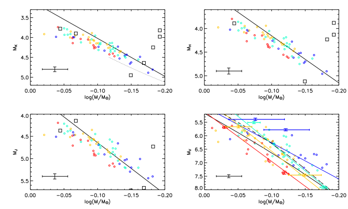
Figure 12: Empirical mass-luminosity relation from Henry & McCarthy (1993) in different bands (solid black line) overplotted to our sample stars. The squares are the stars used by Henry & McCarthy (1993) to fit their empirical mass-luminosity relation. Infrared colours have been converted to the CIT system. Only stars with accurate IR photometry (“j_”$+$“h_”$+$“k_msigcom”$<0.10$) are shown. Points correspond to the sample stars in the range $Z<0.007$ (blue), $0.007\leq Z<0.014$ (cyan), $0.014\leq Z<0.022$ (yellow), $Z\geq 0.022$ (red). The dotted line in the first panel is the Delfosse et al. (2000) empirical relation. The dashed line in the fourth panel is the Kroupa et al. (1993) empirical relation. In the fourth panel are also shown (with colored error bars) the stars of Table 3 with the exception of $\xi$ Boo A and B (see discussion in Section 6), vB22 A and $\eta$ Cas B (outside of the plot range). The coloured lines are fits in the same metallicity bins of the sample stars as explained in the text. A typical error bar for the points is also shown in the lower left of each panel.

The comparison between our data and the empirical mass-luminosity relations is shown in Figure 12. Overall, the agreement is quite good and the data appear to follow the trend of the Henry & McCarthy (1993) relations. In the infrared, the points slightly depart from the empirical formulae at brighter luminosities and masses higher than $\sim 0.85M_{\odot}$ (depending on the band). This might be due to evolutionary effects, however we caution that the Henry & McCarthy (1993) formulae fit rather noisy data; interestingly, when the single stars used by Henry & McCarthy (1993) are overplotted (from their table 5), at higher masses the agreement is good. Therefore, considering the uncertainty in the data and the scatter amongst the empirical relations, the agreement is within $1\sigma$ throughout the entire range. Also, the Henry & McCarthy (1993) mass-luminosity relation is obtained using stars of intermediate disk age with various metallicities so that either of these effects are built in the relations themselves. We also show the relations of Delfosse et al. (2000) (valid for $M_{K}\geq 4.5$) and Kroupa et al. (1993) in the visible. In $V$ band the scatter is much larger, but there is no clear departure from the empirical relations: stars with different metallicities lie in different parts of the mass-luminosity relation, and less so in the infrared. This metallicity dependence is also confirmed when the empirical binary data of Table 3 are overplotted. Such behaviour is predicted by all theoretical models (e.g. Chabrier & Baraffe 2000) and it was also noticed by Delfosse et al. (2000) for stars with masses lower than those covered in the present study.

In the forth panel of Figure 12 a linear fit for the stars of Section 2 in different metallicity bins is shown. Around and above solar metallicity (yellow and red lines) the fit is in outstanding agreement with the binaries of Table 3, whereas a marked difference in the slope appears at low metallicity (although still in agreement with the empirical relation of Henry & McCarthy 1993). Clearly, more empirical masses and luminosities for metal poor binaries would be extremely interestingly. If a steeper slope for metal poor stars is required, that could be achieved by reducing the mass deduced from the isochrones which in turn would imply a higher helium abundance (see Figure 6). Therefore we suggest that more data on the empirical mass-luminosity relation for metal poor stars could help to constrain the helium abundance in stars.

8 The Helium content in planet host stars

Stars with planetary companions have been shown to be, on average, considerably more metal-rich when compared with stars without planets in the solar neighborhood (e.g. Gonzalez 1997, 1998; Santos, Israelian & Mayor 2000; Gonzalez et al. 2001; Santos et al. 2005; Fischer & Valenti 2005). A high degree of statistical significance is obtained when iron is used as the reference element. When other elements are investigated, the situation is much less clear (see e.g. Gonzalez 2003, 2006 for reviews). There is some evidence that planet host stars differ from other nearby stars without planets in their abundances of Mg, Al, Si, V, Co and Ni. As regards the light elements, no significant difference between planet and non planet host stars is found for Be (e.g. Santos et al. 2004b) whereas the situation is more uncertain for Li (e.g. Gonzalez 2006).

Here we attempt for the first time to derive the helium abundance for a small set of planetary host stars. They all have metallicities around or above the solar one, where the isochrones have been proven to be in overall good agreement with the empirical data (see Section 6 and 7).

Our sample of planetary host stars is drawn from the comprehensive list of Santos et al. (2004a) which provides accurate spectroscopic [Fe/H] measurements. Abundances for the $\alpha$-elements are available from the same research group (Gilli et al. 2006). Two planet host stars (HD3651 and HD130322) were in our original sample of Section 2. The other stars have been chosen if accurate $BV(RI)_{C}$ colours (from Bessell 1990) were available so that $T_{eff}$ and bolometric luminosities could be estimated as described in Section 2. If accurate $JHK_{S}$ magnitudes were also available from the 2MASS, the IRFM (Casagrande et al. 2006) has been applied directly. We also used the Hipparcos classification to discard variable stars. The absence of variability ensures that the stars are likely to be chromospherically quiet, so that chromospheric-age relations can be more safely used (Donahue 1998). Most of the planet host stars for which we found accurate metallicities and photometry have $M_{Bol}<5.4$, meaning that evolutionary effects need to be taken into account. For all these stars, age determinations based on chromospheric indices are available from Saffe, Gómez & Chavero (2005). Two calibrations are usually adopted to deduce ages from chromospheric indices: that of Donahue (1993) and that of Rocha-Pinto & Maciel (1998). For a number of reasons, the Donahue (1993) calibration is usually preferred (Feltzing et al. 2001; Saffe et al. 2005) and is adopted here.

The chromospheric-age relation is considered to be rather robust for ages younger than $\sim 6$ Gyr (Saffe et al. 2005). When long-term observations are available –as in Saffe et al. (2005)–, for a given functional form, the age uncertainty can be as small as $\sim 1$ Gyr (Donahue 1998). More serious problems come if a star is actually in a Maunder-minimum state where errors estimates can be as high as 5 Gyr. However there are indications that Maunder-minima are very rare among young stars (e.g. Gustaffson 1999). In our case, planet host stars have a median age of 5.1 Gyr using the Donahue (1993) calibration, consistent with the evidence that most of the nearby solar-type stars have an activity level and age similar to the Sun (Henry et al. 1996). These evolved stars (with typical $M_{Bol}\sim 4.5$) are more sensitive to the age adopted for the isochrones : a variation of 1 Gyr changes masses by $0.04-0.05M_{\odot}$ and helium abundances $Y$ by $0.02-0.03$ on average, about the same order of the uncertainties originating from the errors in $T_{eff}$ and $M_{Bol}$. For evolved stars we therefore sum in quadrature the errors estimated via MonteCarlo (according to the prescription given in Section 4.2) to those resulting from a variation of 1 Gyr in the age of the adopted isochrones. The complete list of planet host stars with their relevant parameters is shown in Table 4.

Table 4: Physical parameters and ages adopted for planet host stars and helium abundances and masses deduced from the isochrones.

HD	$T_{eff}$	$M_{Bol}$	$Z$	Age (Gyr)	$Y$	$\frac{M}{M_{\odot}}$
142	$6247\pm 81$	$3.63\pm 0.05$	$0.023\pm 0.003$	5.93	$0.29\pm 0.04$	$1.07\pm 0.07$
3651	$5191\pm 158$	$5.47\pm 0.07$	$0.023\pm 0.003$	5.13	$0.21\pm 0.06$	$0.97\pm 0.10$
17051	$6067\pm 123$	$4.19\pm 0.05$	$0.028\pm 0.003$	1.47	$0.26\pm 0.07$	$1.20\pm 0.11$
70642	$5667\pm 60$	$4.81\pm 0.04$	$0.027\pm 0.002$	3.88	$0.26\pm 0.03$	$1.04\pm 0.07$
130322	$5429\pm 31$	$5.54\pm 0.10$	$0.017\pm 0.002$	1.24	$0.25\pm 0.03$	$0.86\pm 0.04$
160691	$5689\pm 46$	$4.13\pm 0.04$	$0.031\pm 0.002$	6.41	$0.29\pm 0.03$	$1.08\pm 0.06$
179949	$6205\pm 104$	$4.07\pm 0.05$	$0.024\pm 0.002$	2.05	$0.29\pm 0.06$	$1.13\pm 0.11$
210277	$5556\pm 77$	$4.79\pm 0.04$	$0.026\pm 0.002$	6.93	$0.29\pm 0.05$	$0.95\pm 0.07$

The uncertainty in mass and helium abundance for stars with $M_{bol}<5.4$ is not straightforward to determine since age plays a role, as we discuss in the text. Errors in $M_{bol}$ also account for the uncertainty in parallaxes.

Our results suggest that within the present day accuracy, planet host stars do not show any anomalous helium abundance with respect to other field stars in the same metallicity range. This is in agreement with the fact that $Y_{\odot}$ is recovered within $1\sigma$ from field stars (Table 2). A Kolmogorov-Smirnov test for the helium content between stars with and without planets in the same metallicity range of Table 4 confirm that the two populations are drawn from the same distribution. The number of available data points is still small, with large errorbars; but we expect that in the near future, studies of planet host stars in the lower main sequence will improve on the robustness of this conclusion.

Most of the studies about exoplanets depend quite strongly on the physical properties (mostly radius and mass) of the planet host stars. Such properties are usually obtained from the isochrones. In this study we have proven that at high metallicity (i.e. around solar) the isochrones can be used with some confidence. When our masses are compared to those obtained by Santos et al. (2004a) interpolating isochrones with standard helium abundances, the agreement is usually good with a mean difference $\Delta M=0.04\pm 0.13M_{\odot}$.

9 Conclusions

We have compared a set of K dwarfs with accurate effective temperature $T_{eff}$, metallicity $Z$ and luminosity $M_{bol}$ to a grid of stellar theoretical isochrones, in order to indirectly determine the helium abundance $Y$ in the stars. We then derive the helium-to-metal enrichment ratio $\Delta Y/\Delta Z$ in the Solar Neighbourhood.

For all our stars the fundamental physical parameters were derived empirically and homogeneously, with the specific aim of measuring small differential effects along the lower main sequence (Section 2). The isochrones used are among the most up-to-date, implementing the latest input physics and covering a large grid of $(Y,Z)$ values; also, we have verified that, for similar $(Y,Z)$ content they compare very well to other recent sets (Yonsei-Yale, Teramo and MacDonald) and therefore our results do not depend significantly on the specific isochrones employed (Section 3.2).

While we derive reasonable values for helium content in our K dwarfs around solar metallicity, the isochrones yield very low values of helium in the metal poor K dwarfs. At metallicities around and above the solar, we obtain $\Delta Y/\Delta Z\sim 2$ (Section 4.2), but at low metallicities, the match between the theoretical and observed main sequence is so poor. Theoretical isochrones can be forced to fit metal poor stars only by assuming very low helium abundances, well below the primordial Big-Bang value (Section 4; Figure 7). This result is quite puzzling.

Although different isochrone sets exhibit some differences in the derived helium content (especially at the lowest metallicities and luminosities), very low helium abundances are already found for moderately metal poor and bright stars, where all the isochrones agree remarkably well. The size and homogeneity of the sample of stars, the accuracy in both empirical and theoretical data, together with the possibility of making the comparison directly in the $T_{eff}-M_{Bol}$ plane, where the effect of the helium content are most evident, are the major improvements over similar work in the past.

The helium discrepancy was known to exist (Lebreton et al. 1999) – the present sample greatly extends on previous work and appears to show that there is a clear problem in fitting stellar models to low mass, metal poor stars. Lebreton et al. (1999) showed that adjustments in stellar models (diffusion) and observations (NLTE effects) alleviate the problem but do not solve it, although their conclusions were based on a rather small number of stars.

We also find that diffusion and NLTE are unlikely to solve the problem completely. We rule out systematic errors in our metallicity scale or temperature scale as the culprit, since the systematic errors required would be much larger than our error estimates comfortably allow, and external checks indicate our other derived stellar physical parameters (mass, luminosity and temperature) are excellent. Our very low helium abundances in the metal poor K dwarfs can be avoided via the ad hoc assumption that the mixing-length parameter decreases with decreasing metallicity for $Z$ below solar; this is of course a very major change to make to stellar models.

Interestingly, discrepancies between theory and observations for stars less massive than the Sun have already been reported in the literature from the studies of binaries (e.g. Popper 1997; Torres & Ribas 2002, see Section 6). However, such discrepancies in the range of K dwarfs have not yet caught –in our opinion– the attention they deserve, as most of the studies aiming to empirically measure mass-luminosity relations have preferentially focused on either earlier or later spectral types. We urge stellar model makers to reassess the modeling of low metallicity, lower main sequence stars.

As we have discussed in Section 6, accurate masses and fundamental physical parameters for metal poor dwarf binaries would be a powerful test of stellar models. The slope of the mass-luminosity relation in the metal poor regime could directly test the effect of diffusion (Section 5) and be used to determine the helium abundance (Section 7). Low degree modes from space-based asteroseismology missions can be used to determine the helium abundance in stellar envelopes with an accuracy of 0.03 for a $0.8M_{\odot}$ star (Basu et al. 2004). Such accuracy is comparable to that in the present work. The study of such modes in metal poor dwarfs with on-going or forthcoming space missions like COROT and Kepler is therefore urged.

Theoretical isochrones are extensively used to determine the distance scale fitting the observed colour-magnitude diagram of globular clusters. Metal poor isochrones with primordial, or close to primordial, helium abundance are used to infer their distance. However, our direct observations of nearby stars are challenging low metallicity isochrones : if extremely helium poor isochrones are formally needed to fit empirical data, this would stretch the (isochrone-based) distance scale by $0.1-0.2$ magnitudes (but note that empirically calibrated distance scales based on nearby subdwarfs would remain unaffected). Besides, assuming primordial helium for the metal poor population in such objects would imply, in a differential sense, extremely helium enhanced values for the metal rich counterparts. We stress that here we are not arguing that our very low helium abundances are real; rather we attribute them to the current limits in stellar models. Clearly direct parallaxes measurements for stars in globular clusters (as Gaia and SIM will provide) will shed new light on the problem.

In the meanwhile, more studies for modeling low mass, metal poor stars are needed. At present, the impact of 3D model atmospheres on stellar abundance determinations is revolutionizing the field; the solar model itself is under profound revision, and in coming years we expect many exciting breakthroughs.

Our study shows that at metallicities around and above solar, theoretical models are in good agreement with observations. This is of interest to studies of exoplanets, which are primarily around host stars of about the solar metallicity, since they still heavily depend on theoretical stellar models to constrain properties of the parent star.

Appendix A The metal mass fraction

The metal mass fraction $Z$ is related to the measured abundance [M/H] by

$$\textrm{[M/H]}=\log(Z/X)-\log(Z/X)_{\odot}$$ (4)

where $Z=1-X-Y$ and $X$ and $Y$ are the hydrogen and helium mass fraction, respectively. It follows that for any given star with measured [M/H] the corresponding metal mass fraction is

$$Z=\epsilon\,Z_{\odot}10^{\textrm{[M/H]}}$$ (5)

where

$$\epsilon=\frac{(1-Y)/X_{\odot}}{1+(Z/X)_{\odot}10^{\textrm{[M/H]}}}.$$ (6)

From Figure (13) it is clear that the use of such a correction has negligible effect (few percent) for standard helium values and up to $\sim 25$ percent in the case of an helium abundance as low as $Y=0.10$. For all the stars in our sample, we have computed $Z$ and $Y$ iteratively: $Z=Z_{\odot}\times 10^{\textrm{[M/H]}}$ was used to obtain a first estimate of the metal mass fraction used for interpolating over our grid of isochrones as explained in Section 4. This returned an estimate of $Y$ that was then used into equation (5) and the newly computed metal mass fraction used for another interpolation over our grid of isochrones. The procedure was iterated until $Z$ and $Y$ converged to better than 0.001, usually within $4-5$ iterations.

We have adopted the solar abundances of Section 3.2, but notice that changing from $(Z/X)_{\odot}=0.0236$ to $(Z/X)_{\odot}=0.0245$ affects the final values of $Z$ and $Y$ by less than $10^{-4}$.

Figure 13: Change in metal mass fraction for different [M/H] and helium abundances $Y$.

Appendix B The Lutz-Kelker bias

The Lutz–Kelker bias on the absolute magnitude is in principle present at any level of parallax accuracy. The bias has two components, the first of which is statistical: since the number of stars increases with decreasing parallaxes (i.e. larger distances and sampled volumes) observational errors on the parallax will not cancel out exactly, giving a net effect of more stars with overestimated parallaxes. This makes the correction on the magnitudes of the individual stars statistical and dependent upon the properties of the sample. The second component of the bias arises because distances (and hence absolute magnitudes) are not linear functions of the parallaxes. Even if errors have a normal distribution in parallax, they propagate to a skewed distribution in distance (absolute magnitude). Once again the effect is to favor more distant (brighter) stars to appear closer (fainter). It is clear that this is a correction that has to be applied to the absolute magnitude of individual stars.

In recent literature there is a certain degree of confusion about what exactly is the Lutz–Kelker bias, whether any correction should be applied and, if so, how large it should be. The value of the corrections to be applied depends on the distribution of the true parallaxes $\omega_{0}$. In principle the true parallax distribution could be derived by deconvolving the observed distribution for observational errors. In practice, the deconvolution process is quite uncertain and most of the authors prefer to use analytical formulae for the correction. The most widely used is that of Hanson (1979), who gave analytical formulae relating absolute magnitude corrections to the proper motion distribution of the sample of stars. However, the use of such formulation is highly risky and it does not provide the necessary accuracy because of the strong dependence on the variety of input parameters. As recommended by Brown et al. (1997) in their paper on the properties of the Hipparcos catalog, any correction should be tailored for each specific case. In fact, the blind use of Hanson’s formulation is often counterproductive as noticed already by many authors (Gratton et al. 1997; Sandage & Saha 2002). Assuming a uniform density case, Hanson’s formulation can be used as an estimator for the worst-case scenario, but not as a correction for the bias. Since the Hipparcos catalog completeness decreases with increasing magnitude, the statistical correction is negligible.

On the other hand, since we are dealing with the magnitude difference between individual stars and a reference isochrone, the correction for the skewed distribution is more relevant (at least in principle). Since magnitudes (and distances) are not linear functions of the parallax, one needs to resort to likelihood methods where the complete probability distribution function (pdf) of $\omega$ given its uncertainties, is transformed into the corresponding distribution function for distance and magnitude. By means of such a method we prove the bias to be well within our observational errors.

Assuming a Gaussian distribution for the errors around the measured parallax $\omega$

$$f\left(\tilde{\omega}\right)=\frac{1}{\sqrt{2\pi}\sigma}e^{-\frac{(\tilde{\omega}-\omega)^{2}}{2\sigma^{2}}},$$ (7)

the expectation value for the distance $R$ is

$$E[R|\omega]=\int_{-\infty}^{+\infty}\frac{1}{\tilde{\omega}}f\left(\tilde{\omega}\right)\textrm{d}\tilde{\omega}=\frac{1}{\sqrt{2\pi}\sigma}\int_{-\infty}^{+\infty}g(\tilde{\omega})e^{\frac{t(\tilde{\omega})}{{2\sigma^{2}}}}\textrm{d}\tilde{\omega}$$ (8)

where $g(\tilde{\omega})=1/\tilde{\omega}$ and $t(\tilde{\omega})=-(\tilde{\omega}-\omega)^{2}$. Defining $u=\tilde{\omega}-\omega$ and expanding $g(\tilde{\omega})$ around the maxima of $t(\tilde{\omega})$ one gets the following series

$$g(\tilde{\omega})=\frac{1}{\omega}\sum_{n=0}^{\infty}(-1)^{n}\left(\frac{u}{\omega}\right)^{n}.$$ (9)

Given the accuracy of our parallaxes, the condition $|u/\omega|<1$ for the expansion is certainly satisfied within, say, $3\sigma$. The choice of the $3\sigma$ cutoff sounds perfectly reasonable for the purposes of our calculation. Alternatively, a more rigorous approach has been investigated by Smith & Eichhorn (1996).

Once the series expansion for $g(\tilde{\omega})$ is known, the integral in eq. (8) reads

$$E[R|\omega]=\frac{1}{\sqrt{2\pi}\sigma}\int_{-\infty}^{+\infty}\frac{1}{\omega}\sum_{n=0}^{\infty}(-1)^{n}\left(\frac{u}{\omega}\right)^{n}e^{-\frac{u^{2}}{2\sigma^{2}}}\textrm{d}u$$ (10)

and can easily be calculated by using Gaussian integrals and noticing that odd terms vanish. The result is the following series

$$E[R|\omega]=\frac{1}{\omega}\sum_{n=0}^{\infty}\frac{(2n)!}{2^{n}n!}\left(\frac{\sigma}{\omega}\right)^{2n}$$ (11)

and the amplitude of the bias

$$E[R|\omega]-\frac{1}{\omega}\sim\frac{1}{\omega}\left(\frac{\sigma}{\omega}\right)^{2}$$ (12)

can be easily checked to be negligible for our adopted accuracy in parallaxes (6%).

In the same manner we can give an estimate for the bias in absolute magnitudes $M_{\xi}$ in a given band $\xi$ or bolometric. We thus have

$$E[M_{\xi}|\omega]=\frac{1}{\sqrt{2\pi}\sigma}\int_{-\infty}^{+\infty}g(\tilde{\omega})e^{\frac{t(\tilde{\omega})}{{2\sigma^{2}}}}\textrm{d}\tilde{\omega},$$ (13)

where now, for a given apparent magnitude $\xi$, we have

$$g(\tilde{\omega})=\xi+5\log(\tilde{\omega})-10.$$ (14)

Hence the integral to be computed is

$$E[M_{\xi}|\omega]=\frac{1}{\sqrt{2\pi}\sigma}\int_{-\infty}^{+\infty}\Big{[}\xi+5\log(\omega)-10+$$

$$\phantom{E[M_{\xi}|\omega]=}5\log(e)\sum_{n=1}^{\infty}\frac{(-1)^{n+1}}{n}\left(\frac{u}{\omega}\right)^{n}\Big{]}e^{-\frac{u^{2}}{2\sigma^{2}}}\textrm{d}u$$ (15)

and gives the following bias

$$E[M_{\xi}|\omega]-M_{\xi}=-5\log(e)\sum_{n=1}^{\infty}\frac{(2n-1)!}{2^{n}n!}\left(\frac{\sigma}{\omega}\right)^{2n}.$$ (16)

Also for the absolute magnitudes the bias is negligible. At the first order the above equation gives

$$E[M_{\xi}|\omega]-M_{\xi}=-\frac{5}{2}\log(e)\left(\frac{\sigma}{\omega}\right)^{2}\sim-0.004\;\textrm{mag}$$ (17)

in the case of lowest parallax accuracy and thus well within our observational errors.

We finally note that given the high precision of our parallaxes ($\sigma/\omega\leq 0.06$) a fully Bayesian approach is not needed, also considering that it would require a priori assumptions on the parameter distributions. A Bayesian approach is indeed demanded for lower precision parallaxes and it has been extensively studied by Smith (1985, 1987, 2003) in his series of papers on the Lutz–Kelker bias.

References

- Allende Prieto (1999) Allende Prieto C., Lambert D.L., 1999, A&A, 352, 555
- Allende Prieto (1999) Allende Prieto C.,García López R., Lambert D.L., Gustafsson B., 1999, ApJ, 527, 879
- Allende-Prieto (2004) Allende Prieto C., Barklem P.S., Lambert D.L., Cunha K., 2004, A&A, 420, 183
- Alonso (1995) Alonso A., Arribas S., Martínez-Roger C., 1995, A&A, 297, 197
- Alonso (1996a) Alonso A., Arribas S., Martínez-Roger C., 1996a, A&A, 117, 227
- Alonso (1996b) Alonso A., Arribas S., Martínez-Roger C., 1996b, A&A, 313, 873
- An (2007) An D., Terndrup D.M., Pinsonneault M.H., Paulson D.B., Hanson R.B., Stauffer J.T., 2007, ApJ, 655, 233
- Andersen (1991) Andersen J., 1991, A&AR, 3, 91
- Antia (2005) Antia H.M., Basu S., 2005, ApJ, 620, 129
- Asplund (2005) Asplund M., 2005, ARA&A, 43, 481
- Asplund (2005) Asplund M., Grevesse N., Sauval A.J., 2005, in Barnes T.G., III, Bash F. N., eds, ASP Conf. Ser. Vol. 336, Cosmic Abundances as Records of Stellar Evolution and Nucleosynthesis, p.25
- Asplund (2006) Asplund M., Lambert D.L., Nissen P.E., Primas F., Smith V.V., 2006, ApJ, 644, 229
- Bahcall (1995) Bahcall J.N., Pinsonneault M.H., Wasserburg G.J., 1995, Rev Mod Phys, 67, 781
- Bahcall (1997) Bahcall J.N., Pinsonneault M.H., Basu S., Christensen-Dalsgaard J., 1997, Phys.Rev.Lett., 78, 171
- Bahcall (2006) Bahcall J.N. Serenelli A.M., Basu S., 2006, ApJS, 165, 400
- Baliunas (1995) Baliunas S.L. et al., 1995, ApJ, 438, 269
- Balser (2006) Balser D.S., 2006, AJ, 132, 2326
- Basu (2004) Basu S., Antia H.M., 2004, ApJ, 606, 85
- Basu (2000) Basu S., Pinsonneault M.H., Bahcall J.N., 2000, ApJ, 529, 1084
- Basu (2004) Basu S., Mazumdar A., Antia H.M., Demarque P., 2004, MNRAS, 350, 277
- Bedin (2004) Bedin L.R., Piotto G., Anderson J., Cassisi S., King I.R., Momany Y., Carraro G., 2004, ApJ, 605, 125
- Bessell (1979) Bessell M. S., 1979, PASP, 91, 589
- Bessell (1990) Bessell M. S., 1990, A&AS, 83, 357
- Bessell (1995) Bessell M. S., 1995, PASP, 107, 672
- Bessell (2000) Bessell M. S., 2000, PASP, 112, 961
- Bigot (2006) Bigot L., Kervella P., Thévenin F., Ségransan D., 2006, A&A, 446, 635
- Boden (2006) Boden A.F., Torres G., Latham D.W., 2006, ApJ, 644, 1193
- Bonfils (2005) Bonfils X., Delfosse X., Udry S., Santos N.C., Forveille T., Ségransan D., 2005, A&A, 442, 635
- Bonifacio (2007) Bonifacio et al., 2007, A&A, 462, 851
- Bressan (1993) Bressan A., Fagotto F., Bertelli G., Chiosi C., 1993, A&AS, 100, 647
- Brown (1997) Brown A.G.A., Arenou F., van Leeuwen F., Lindegren L., Luri X., 1997, Hipparcos - Venice 1997 Proc., ESA SP-402. ESA Publications Division, Noordwijk, p.63
- Brun (1999) Brun A.S., Turck-Chièze S., Zahn J.P., 1999, ApJ, 525, 1032
- Caloi (2007) Caloi V., D’Antona F., 2007, A&A, 463, 949
- Carpenter (2001) Carpenter J.M., 2001, AJ, 121, 2851
- Carrier (2006) Carrier F., Eggenberger P., 2006, A&A, 450, 695
- Casagrande (2006) Casagrande L., Portinari L., Flynn C., 2006, MNRAS, 373, 13
- Castellani (1997) Castellani V., Ciacio F., degl’Innocenti S., Fiorentini G., 1997, A&A, 322, 801
- Castellani (1999) Castellani V., degl’Innocenti S., Marconi M., 1999, A&A, 349, 834
- Catchpole (2007) Catchpole R.M., Pagel B.E.J., Powell A.L.T., 1967, MNRAS, 136, 403
- Chaboyer (1994) Chaboyer B., Demarque P., 1994, ApJ, 433, 510
- Chaboyer (1992) Chaboyer B., Deliyannis C.P., Demarque P., Pinsonneault M.H., Sarajedini A., 1992, ApJ, 388, 372
- Chaboyer (2001) Chaboyer B., Fenton W.H., Nelan J.E., Patnaude D.J., Simon F.E., 2001, ApJ, 562, 521
- Chabrier (2000) Chabrier G., Baraffe I., 2000, ARA&A, 38, 337
- Chiappini (2002) Chiappini C., Renda A., Matteucci F., 2002, A&A 395, 789
- Chieffi (1995) Chieffi A., Straniero O., Salaris M., 1995, ApJ, 445, 39
- Chiosi (1982) Chiosi C., Matteucci F., 1982, A&A, 105, 140
- Claret (1995) Claret A., 1995, A&AS, 109, 441
- Cordier (2007) Cordier D., Pietrinferni A., Cassisi S., Salaris M., 2007, AJ, 133, 468
- Cox (1968) Cox J.P., Giuli R.T., 1968, Principles of Stellar Structure. Gordon & Breach, New York
- Christensen-Dalsgaard (1993) Christensen-Dalsgaard J., Proffitt C.R., Thompson M.J., 1993, ApJ, 403, 75
- D’Antona (2005a) D’Antona F., Bellazzini M., Caloi V., Pecci F.F., Galleti S., Rood R.T., 2005a, ApJ, 631, 868
- D’Antona (2005b) D’Antona F., Cardini D., Di Mauro M.P., Maceroni C., Mazzitelli I., Montalbán J., 2005b, MNRAS, 363, 847
- de Bruijne (2001) de Bruijne J.H.J., Hoogerwerf R., de Zeeuw P.T., 2001, A&A, 367, 111
- Delahaye (2006) Delahaye F., Pinsonneault M.H., 2006, ApJ, 649, 529
- Delfosse (2000) Delfosse X., Forveille T., Ségransan D., Beuzit J.-L., Udry S., Perrier C., Mayor M., 2000, A&A, 364, 217
- Deliyannis (1991) Deliyannis C.P., Demarque P., 1991, ApJ, 370, 89
- Demarque (2004) Demarque P., Woo J.-H., Kim Y.-C., Yi S.K., 2004, ApJS, 155, 667
- Dennis (1965) Dennis T.R., 1965, PASP, 77, 283
- Donahue (1993) Donahue R.A., 1993, Ph.D. Thesis, New Mexico State University
- Donahue (1998) Donahue R.A., 1998, in Stellar Systems and the Sun, ed. R.A. Donahue, & J. A. Bookbinder, ASP Conf. Ser., 154, 1235
- Drummond (1995) Drummond J.D., Christou J.C., Fugate R.Q., 1995, ApJ, 450, 380
- Edmonds (1992) Edmonds P., Cram L., Demarque P., Guenther D.B., Pinsonneault M.H., 1992, ApJ, 394, 313
- Eggen (1968) Eggen O.J., 1968, Roy. Obs. Bull., No. 137
- Eggen (1973) Eggen O.J., 1973, ApJ, 182, 821
- Eggen (1975) Eggen O.J., 1975, PASP, 87, 107
- Eggen (1979) Eggen O.J., 1979, ApJS, 39, 89
- Eggenberger (2004) Eggenberger P., Charbonnel C., Talon S., Meynet G., Maeder A., Carrier F., Bourban G., 2004, A&A, 417, 235
- Fabricius (2000) Fabricius C., Makarov V.V., 2000, A&A, 356, 141
- Faulkner (1967) Faulkner J., 1967, ApJ, 147, 617
- Feltzing (2001) Feltzing S., Gonzalez G., 2001, A&A, 367, 253
- Feltzing (2001) Feltzing S., Holmberg J., Hurley J.R., 2001, A&A, 377, 911
- Fernandes (1995) Fernandes J., Neuforge C., 1995, A&A, 295, 678
- Fernandes (2004) Fernandes J., Santos N.C., 2004, A&A, 427, 607
- Fernandes (1996) Fernandes J., Lebreton Y., Baglin A., 1996, A&A, 311, 127
- Fernandes (1998) Fernandes J., Lebreton Y., Baglin A., Morel P., 1998, A&A, 338, 455
- Fernandes (2002) Fernandes J., Morel P., Lebreton Y., 2002, A&A, 392, 529
- Fernie (1983) Fernie J.D., 1983, PASP, 95, 782
- Ferraro (2004) Ferraro F.R., Sollima A., Pancino E., Bellazzini M., Straniero O., Origlia L., Cool A.M., 2004, ApJ, 603, 81
- Ferraro (2006) Ferraro F.R., Valenti E., Straniero O., Origlia L., 2006, ApJ, 642, 225
- Fischer (2005) Fischer D.A., Valenti J., 2005, ApJ, 622, 1102
- Fulbright (2000) Fulbright J.P., 2000, AJ, 120, 1841
- Fuhrmann (2004) Fuhrmann K., 2004, AN, 325, 3
- Gallart (2005) Gallart C., Zoccali M., Aparicio A., 2005, ARA&A, 43, 387
- Gehren (2001a) Gehren T., Butler K., Mashonkina L., Reetz J., Shi J., 2001a, 366, 981
- Gehren (2001b) Gehren T., Korn A.J., Shi J., 2001b, A&A, 380, 645
- Gilli (2006) Gilli G., Israelian G., Ecuvillon A., Santos N.C., Mayor M., 2006, A&A, 449, 723
- Girardi (2000) Girardi L., Bressan A., Bertelli G., Chiosi C., 2000, A&AS, 141, 371
- Girardi (2007) Girardi L., Castelli F., Bertelli G., Nasi E., 2007, A&A, 468, 657
- Glebocki (2000) Glebocki R., Stawikowski A., 2000, Acta Astron., 50, 509
- Gliese (1991) Gliese W., Jahreiß H., 1991, Catalogue of Nearby Stars. 3rd edn, Astron. Rechen-Institut, Heidelberg
- Gonzalez (1997) Gonzalez G., 1997, MNRAS, 285, 403
- Gonzalez (1998) Gonzalez G., 1998, A&A, 334, 221
- Gonzalez (2003) Gonzalez G., 2003, Rev. Mod. Phys., 75, 101
- Gonzalez (2006) Gonzalez G., 2006, PASP, 118, 1494
- Gonzalez (2001) Gonzalez G., Laws C., Tyagi S., Reddy B.E., 2001, AJ, 121, 432
- Gratton (1997) Gratton R.G., Fusi Pecci F., Carretta E., Clementini G., Corsi C.E., Lattanzi M., 1997, ApJ, 491, 749
- Gratton (1999) Gratton R.G., Carretta E., Eriksson K., Gustafsson B., 1999, A&A, 350, 955
- Gratton (2001) Gratton R.G. et al., 2001, A&A, 369, 87
- Gratton (2003) Gratton R.G., Carretta E., Claudi R., Lucatello S., Barbieri M., 2003, A&A, 404, 187
- Gratton (2004) Gratton R., Sneden C., Carretta E., 2004, ARA&A, 42, 385
- Grevesse (1993) Grevesse N., Noels A., 1993, Phys. Scr. T, 47, 133
- Griffin (2004) Griffin R.F., 2004, Obs., 124, 258
- Guenther (1997) Guenther D.B., Demarque P., 1997, ApJ, 484, 937
- Guenther (2000) Guenther D.B., Demarque P., 2000, ApJ, 531, 503
- Gustafsson (1999) Gustafsson B., 1999, ed. I. Hybeny, S. Heap, & R. Cornett, ASP Conf. Ser., 192, 91
- Hall (1948) Hall R.G.J., 1948, AJ, 54, 102
- Hanson (1979) Hanson R.B., 1979, MNRAS, 186, 875
- Haywood (1992) Haywood J.W., Hegyi D.J., Gudehus D.H., 1992, ApJ, 392, 172
- Hegyi (1970) Hegyi D., Curott D., 1970, Phys. Rev. Lett., 24, 415
- Heintz (1993) Heintz W.D., 1993, AJ, 105, 1188
- Henry (1993) Henry T.J., McCarthy D.W.J., 1993, AJ, 106, 773
- Henry (1996) Henry T.J., Soderblom D.R., Donahue R.A., Baliunas S.L., 1996, AJ, 111, 439
- Henry (1999) Henry T.J., Franz O.G., Wasserman L.H., Benedict G.F., Shelus P.J., Ianna P.H., Kirkpatrick J.D., McCarthy D.W.J., 1999, ApJ, 512, 864
- Henry (2006) Henry G.W., Fekel F.C., Sowell J.R., Gearhart J.S., 2006, AJ, 132, 2489
- Holmberg (2006) Holmberg J., Flynn C., Portinari L., 2006, MNRAS, 367, 449
- Izotov (2007) Izotov Y.I., Thuan T.X., Stasinska G., 2007, ApJ, 662, 15
- Jimenez (1996) Jimenez R., MacDonald J., 1996, MNRAS, 283, 721
- Jimenez (1996) Jimenez R., Thejll P., Jorgensen U.G., MacDonald J., Pagel B., 1996, MNRAS, 282, 926
- Jimenez (1998) Jimenez R., Flynn C., Kotoneva E., 1998, MNRAS, 299, 515
- Jimenez (2002) Jimenez R., Loeb A., 2002, ApJ, 573, 37
- Jimenez (2003) Jimenez R., Flynn C., MacDonald J., Gibson B.K., 2003, Sci, 299, 1552
- Jones (1972) Jones B.F., 1972, ApJ, 171, 57
- Kaviraj (2007) Kaviraj S., Sohn S.T., O’Connell R.W., Yoon S.-J., Lee Y.W., Yi S.K., 2007, MNRAS, 377, 987
- Kervella (2004) Kervella P., Thévenin F., Di Folco E., Ségransan D., 2004, A&A, 426, 297
- Kjeldsen (2005) Kjeldsen H. et al., 2005, ApJ, 635, 1281
- Korn (2003) Korn A.J., Shi J., Gehren T., 2003, A&A, 407, 691
- Kotoneva (2002) Kotoneva E., Flynn C., Chiappini C., Matteucci F., 2002, MNRAS, 336, 879
- Kroupa (1993) Kroupa P., Tout C.A., Gilmore G., 1993, MNRAS, 262, 545
- Lacy (2005) Lacy C.H.S., Torres G., Claret A., Vaz L.P.R., 2005, AJ, 130, 2838
- Lastennet (2003) Lastennet E., Fernandes J., Valls-Gabaud D., Oblak E., 2003, A&A, 409, 611
- Lebreton (1999) Lebreton Y., Perrin M-N., Cayrel R., Baglin A., Fernandes J., 1999, A&A, 350, 587
- Lebreton (2000) Lebreton Y., 2000, ARA&A, 38, 35
- Lebreton (2001) Lebreton Y., Fernandes J., Lejeune T., 2001, A&A, 374, 540
- Luck (2006) Luck R.E., Heiter U., 2006, AJ, 131, 3069
- Ludwig (1999) Ludwig H.-G., Freytag B., Steffen M., 1999, A&A, 346, 111
- Lee (1999) Lee Y.-W., Joo J.-M., Sohn Y.-J., Rey S.-C., Lee H.-C., Walker A.R., 1999, Nat, 402, 55
- Lutz (1973) Lutz T.E., Kelker D.H., 1973, PASP, 85, 573
- Maeder (1992) Maeder A., 1992, A&A 264, 105
- Maeder (1993) Maeder A., 1993, A&A 268, 833
- McCarthy (1993) McCarthy D.J. et al., 1993, AJ, 105, 652
- Mermilliod (1997) Mermilliod J.-C., Mermilliod M., Hauck B., 1997, A&AS, 124, 349
- Michaud (1983) Michaud G., Vauclair G., Vauclair S., 1983, ApJ, 267, 256
- Miglio (2005) Miglio A., Montalbán J., 2005, A&A, 441, 615
- Mishenina (2004) Mishenina T.V., Soubiran C., Kovtyukh V.V., Korotin S.A., 2004, A&A, 418, 551
- Moehler (1999) Moehler S., Sweigart A. V., Landsman W. B., Heber U., Catelan M., 1999, A&A, 346, 1
- Morel (1999) Morel P., Baglin A., 1999, A&A, 345, 156
- Morel (2002) Morel P., Thévenin F., 2002, A&A, 390, 611
- Morel (2000a) Morel P., Morel C., Provost J., Berthomieu G., 2000a, A&A, 354, 636
- Morel (2000b) Morel P., Provost J., Lebreton Y., Thévenin F., Berthomieu G., 2000b, A&A, 363, 675
- Neuforge (1993) Neuforge C., 1993, A&A, 268, 650
- Noels (1991) Noels A., Grevesse N., Magain P., Neuforge C., Baglin A., Lebreton Y., 1991, A&A, 247, 91
- Norris (2004) Norris J.E., 2004, ApJ, 612, 25
- Pagel (1998) Pagel B.E.J., Portinari L., 1998, MNRAS, 298, 747
- Palmieri (2002) Palmieri R., Piotto G., Saviane I., Girardi L., Castellani V., 2002, A&A, 392, 115
- Pancino (2000) Pancino E., Ferraro F.R., Bellazzini M., Piotto G., Zoccali M., 2000, ApJ, 534, 83
- Pancino (2002) Pancino E., Pasquini L., Hill V., Ferraro F.R., Bellazzini M., 2002, ApJ, 568, 101
- Pasinetti Fracassini (2001) Pasinetti Fracassini L.E., Pastori L., Covino S., Pozzi A., 2001, A&A, 367, 521
- Paulson (2003) Paulson D.B., Sneden C., Cochran W.D., 2003, AJ, 125, 3185
- Peimbert (2007) Peimbert M., Luridiana V., Peimbert A., 2007, preprint(astro-ph/0701580)
- Perrin (1977) Perrin M.-N., de Strobel G.C., Cayrel R., Hejlesen P.M., 1977, A&A, 54, 779
- Perryman (1998) Perryman M.A.C. et al., 1998, A&A, 331, 81
- Peterson (1979) Peterson R.C., Carney B.W., 1979, ApJ, 231, 762
- Petit (2005) Petit P. et al., 2005, MNRAS, 361, 837
- Pietrinferni (2004) Pietrinferni A., Cassisi S., Salaris M., Castelli F., 2004, ApJ, 612, 168
- Pinsonneault (1992) Pinsonneault M.H., Deliyannis C.P., Demarque P., 1992, ApJS, 78, 179
- Pinsonneault (1999) Pinsonneault M.H., Walker T.P., Steigman G., Narayanan V.K., 1999, ApJ, 527, 180
- Pinsonneault (2002) Pinsonneault M.H., Steigman G., Walker T.P., Narayanan V.K., 2002, ApJ, 574, 398
- Pinsonneault (2003) Pinsonneault M.H., Terndrup D.H., Hanson R.B., Stauffer J.R., 2003, ApJ, 598, 588
- Pinsonneault (2004) Pinsonneault M.H., Terndrup D.H., Hanson R.B., Stauffer J.R., 2004, ApJ, 600, 946
- Popper (1997) Popper D.M., 1997, 114, 1195
- Pourbaix (2002) Pourbaix D. et al., 2002, A&A, 386, 280
- Ramírez (2005) Ramírez I., Meléndez J., 2005, ApJ, 626, 465
- Reid (2007) Reid I.N., Turner E.L., Turnbull M.C., Mountain M., Valenti J.A., 2007, ApJ, 665, 767
- Ribas (2000) Ribas I., Jordi C., Torra J., Giménez A., 2000, MNRAS, 313, 99
- Richard (2002) Richard O., Michaud G., Richer J., Turcotte S., Turck-Chièze S., VandenBerg D.A., 2002, ApJ, 568, 979
- Richard (2005) Richard O., Michaud G., Richer J., 2005, ApJ, 619, 538
- Rocha-Pinto (1998) Rocha-Pinto H., Maciel W., 1998, MNRAS, 298, 332
- Ryan (1996) Ryan S.G., Beers T.C., Deliyannis C.P., Thorburn J.A., 1996, ApJ, 458, 543
- Ryan (1999) Ryan S.G., Norris J.E., Beers T.C., 1999, ApJ, 523, 654
- Saffe (2005) Saffe C., Gómez M., Chavero C., 2005, A&A, 443, 609
- Salaris (2001) Salaris M., Weiss A., 2001, A&A, 376, 955
- Salaris (2000) Salaris M., Groenewegen M.A.T., Weiss A., 2000, A&A, 355, 299
- Salaris (2004) Salaris M., Riello M., Cassisi S., Piotto G., 2004, A&A, 420, 911
- Salasnich (2000) Salasnich B., Girardi L., Weiss A., Chiosi C., 2000, A&A, 361, 1023
- Sandage (2002) Sandage A., Saha A., 2002, AJ, 123, 2047
- Sandquist (2000) Sandquist E.L., 2000, MNRAS, 313, 571
- Santos (2000) Santos N.C., Israelian G., Mayor M., 2000, A&A, 363, 228
- Santos (2004a) Santos N.C., Israelian G., Mayor M., 2004a, A&A, 415, 1153
- Santos (2004b) Santos N.C., Israelian G., García López R.J., Mayor M., Rebolo R., Randich S., Ecuvillon A., Domínguez Cerdeña C., 2004b, A&A, 427, 1085
- Santos (2005) Santos N.C., Israelian G., Mayor M., Bento J.P., Almeida P.C., Sousa S.G., Ecuvillon A., 2005, A&A, 437, 1127
- Schiller (1987) Schiller S.J., Milone E.F., 1987, AJ, 93, 1471
- Schmitt (2004) Schmitt J.H.M.M., Liefke C., 2004, A&A, 417, 651
- Smith (1985) Smith H.J., 1985, A&A, 152, 413
- Smith (1987) Smith H.J., 1987, A&A, 188, 233
- Smith (2003) Smith H., 2003, MNRAS, 338, 891
- Smith (1996) Smith H.J., Eichhorn H., 1996, MNRAS, 281, 211
- Spergel (2007) Spergel D.N. et al., 2007, ApJS, 170, 377
- Spite (1982) Spite F., Spite M., 1982, A&A, 115, 357
- Stauffer (1987) Stauffer J.R., Hartmann L.W., 1987, ApJ, 318, 337
- Stauffer (2003) Stauffer J.R., Jones B.F., Backman D., Hartmann L.W., Barrado y Navascués D., Pinsonneault M.H., Terndrup D.M., Muench A.A., 2003, AJ, 126, 833
- Straniero (1997) Straniero O., Chieffi A., Limongi M., 1997, ApJ, 490, 425
- Söderhjelm (1999) Söderhjelm S., 1999, A&A, 341, 121
- ten Brummelaar (2000) ten Brummelaar T.A., Mason B.D., McAlister H.A., Roberts L.C.J., Turner N.H., Hartkopf W.I., Bagnuolo W.G.J., 2000, AJ, 119, 2403
- Terndrup (2000) Terndrup D.M., Stauffer J.R., Pinsonneault M.H., Sills A., Yuan Y., Jones B.F., Fischer D., Krishnamurthi A., 2000, AJ, 119, 1303
- Thévenin (1999) Thévenin F., Idiart T.P., 1999, ApJ, 521, 753
- Thévenin (2002) Thévenin F., Provost J., Morel P., Berthomieu G., Bouchy F., Carrier F., 2002, A&A, 392, 9
- Thorburn (1994) Thorburn J.A., 1994, ApJ, 421, 318
- Torres (2002a) Torres G., Ribas I., 2002, ApJ, 567, 1140
- Torres (2002) Torres G., Boden A., Latham D.W., Pan M., Stefanik R.P., 2002, AJ, 124, 1716
- Torres (2006) Torres G., Lacy C.H., Marschall L.A., Sheets H.A., Mader J.A., 2006, ApJ, 640, 1018
- Trampedach (1999) Trampedach R., Stein R.F., Christensen-Dalsgaard J., Nordlund Å., 1999, in Gimenez A., Guinan E.F., Montesinos B., eds, ASP Conf. Ser. Vol. 173, Theory and Tests of Convection in Stellar Structure. Astron. Soc. Pac., San Francisco, p.233
- Trotta (2004) Trotta R., Hansen S.H., 2004, Phys. Rev. D, 69, 023509
- Underhill (1963) Underhill A.B., 1963, Pub. Dominion Astrophys. Obs., 12, 159
- Valenti (2005) Valenti J.A., Fischer D.A., 2005, ApJS, 159, 141
- van Leeuwen (1986) van Leeuwen F., Alphenaar P., Brand J., 1986, A&AS, 65, 309
- van Leeuwen (1987) van Leeuwen F., Alphenaar P., Meys J.J.M., 1987, A&AS, 67, 483
- VandenBerg (1984) VandenBerg D.A., Bridges T.J., 1984, ApJ, 278, 679
- VandenBerg (2006) VandenBerg D.A., Bergbusch P.A., Dowler P.D., 2006, ApJS, 162, 375
- Vauclair (1988) Vauclair S., 1988, ApJ, 335, 971
- Vauclair (1995) Vauclair S., Charbonnel C., 1995, A&A, 295, 715
- Weis (1983) Weis E.W., 1983, PASP, 95, 29
- Weis (1996) Weis E.W., 1996, AJ, 112, 2300
- Weiss (1999) Weiss A., Salaris M., 1999, A&A, 346, 897
- Wood (2006) Wood B.E., Linsky J.L., 2006, ApJ, 643, 444
- Yildiz (2007) Yildiz M., 2007, MNRAS, 374, 1264
- Yildiz (2006) Yildiz M., Yakut K., Bakiş H., Noels A., 2006, MNRAS, 368, 1941