New constraints on the observable inflaton potential from WMAP and SDSS

Abstract

We derive some new constraints on single-field inflation from the Wilkinson Microwave Anisotropy Probe 3-year data combined with the Sloan Luminous Red Galaxy survey. Our work differs from previous analyses by focusing only on the observable part of the inflaton potential, or in other words, by making absolutely no assumption about extrapolation of the potential from its observable region to its minimum (i.e., about the branch of the potential responsible for the last $\sim$50 inflationary e-folds). We only assume that inflation starts at least a few e-folds before the observable Universe leaves the Hubble radius, and that the inflaton rolls down a monotonic and regular potential, with no sharp features or phase transitions. We Taylor-expand the inflaton potential at order $v=2$, 3 or 4 in the vicinity of the pivot scale, compute the primordial spectra of scalar and tensor perturbations numerically and fit the data. For $v>2$, a large fraction of the allowed models is found to produce a large negative running of the scalar tilt, and to fall in a region of parameter space where the second-order slow-roll formalism is strongly inaccurate. We release a code for the computation of inflationary perturbations which is compatible with cosmomc.

Cosmological inflation is known to be a successful paradigm providing self-consistent initial conditions to the standard cosmological scenario Starobinsky (1980); Guth (1981); Sato (1981); Hawking and Moss (1982); Linde (1982a, 1983) and explaining the generation of primordial cosmological perturbations Starobinsky (1979); Hawking (1982); Starobinsky (1982); Guth and Pi (1982); Linde (1982b); Bardeen et al. (1983); Abbott and Wise (1984); Salopek et al. (1989). The distribution of Cosmic Microwave Background (CMB) anisotropies, as observed for instance by the Wilkinson Microwave Anisotropy Probe (WMAP) Spergel et al. (2006); Page et al. (2006); Hinshaw et al. (2006); Jarosik et al. (2006), is compatible with the simplest class of inflationary models called single-field inflation.

The definition of single-field inflation is not unique: for instance, some authors consider hybrid inflation Linde (1991, 1994); Copeland et al. (1994) as a multi-field model, since it involves one scalar field in addition to the inflaton field (the role of the second field being to trigger the end of inflation). In this work, we call single-field inflation any model in which the observable primordial spectrum of scalar and tensor metric perturbations can be computed using the equation of motion of a single field. This definition does include usual models of hybrid inflation.

The goal of this paper is to derive from up-to-date cosmological data some constraints on the scalar potential $V(\phi)$ of single-field inflation. This question has already been addressed in many interesting works since the publication of WMAP 3-year results Spergel et al. (2006); Peiris and Easther (2006a); de Vega and Sanchez (2006); Easther and Peiris (2006); Kinney et al. (2006); Martin and Ringeval (2006); Covi et al. (2006); Finelli et al. (2006); Peiris and Easther (2006b); Destri et al. (2007); Ringeval (2007); Cardoso (2007) (see also Cline and Hoi (2006) for earlier results). Our approach is however different, since all these references assume either that the slow-roll formalism can be applied (at first or second order), or that the scalar potential can be extrapolated from the region directly constrained by the data till the end of inflation. We want to relax these two restrictions simultaneously, and to derive constraints on the observable part of the inflaton potential under the only assumption that $V(\phi)$ is smooth enough for being Taylor-expanded at some low order in the region of interest. In this respect, our work is still not completely general and does not explore possible sharp features in the inflaton potential (see e.g. Martin and Ringeval (2006); Covi et al. (2006) for recent proposals). Throughout the abundant literature on the inflaton potential reconstruction, the work following the closest methodology to ours is the pre-WMAP paper of Grivell and Liddle Grivell and Liddle (2000).

The question of whether the slow-roll formalism can be safely employed or not is intimately related to the magnitude of a possible running of the tilt in the primordial spectrum of curvature perturbations. In order to clarify this point, lets us first recall that the slow-roll formalism Steinhardt and Turner (1984); Salopek and Bond (1990); Liddle et al. (1994) consists in employing analytical expressions for the primordial spectrum of curvature perturbations ${\cal P}_{\cal R}(k)$ and gravitational waves ${\cal P}_{h}(k)$. Such expressions hold in the limit in which the first and second logarithmic derivative of the Hubble parameter $H$ with respect to the e-fold number $N\equiv\ln a$ remain smaller than one throughout the $\Delta N\sim 10$ observable e-folds of inflation (i.e., over the period during which observable Fourier modes cross the Hubble radius). Deep inside this limit, the primordial spectra are given by

$${\cal P}_{\cal R}(k)\simeq-\frac{H^{2}}{\pi m_{P}^{2}(d\ln H/dN)}~{},\quad{\cal P}_{h}(k)\simeq-\frac{16H^{2}}{\pi m_{P}^{2}}~{},$$ (1)

where the right-hand sides are evaluated at Hubble crossing. The first-order expression of the scalar/tensor tilts $n_{S,T}$ and tilt runnings $\alpha_{S,T}$ can be easily obtained by taking the derivative of the above expressions, using the slow-roll approximation $d/d\ln k\simeq d/dN$. The derivation of higher-order expressions is more involved (see e.g. Stewart and Lyth (1993); Lidsey et al. (1997); Gong and Stewart (2001); Dodelson and Stewart (2002); Schwarz et al. (2001); Stewart (2002); Leach et al. (2002); Hansen and Kunz (2002); Caprini et al. (2003); Liddle (2003); Choe et al. (2004); Habib et al. (2005); Joy et al. (2005); Kadota et al. (2005); Casadio et al. (2006); de Oliveira and Terrero-Escalante (2006)).

Figure 1: Observable region of the inflaton potential allowed at the 95% C.L. by the WMAP 3-year and Sloan Luminous Red Galaxy survey (SDSS-LRG) data, for a Taylor expansion of the potential at order $v=2$ (top), $v=3$ (middle) or $v=4$ (bottom), in the vicinity of the pivot value $\phi_{*}$. In all diagrams the potentials are normalized to their value at the pivot scale $\phi_{*}$. For clarity, in the right diagrams, the field is expressed in units of $|V_{*}/V^{\prime}_{*}|$ instead of $m_{P}$, so all curves have by definition the same slope in $\phi=\phi_{*}$. In practice, these plots show the superposition of 95% of the potentials from our MCMC chains with the best likelihood (after removal of the burn-in phase). Each potential is plotted in a range $[\phi_{1},\phi_{2}]$ corresponding to Hubble exit for modes in the range $[k_{1},k_{2}]$=$[2\times 10^{-4},0.1]~{}$Mpc^-1 which is most constrained by the data. This corresponds roughly to a history of 6.2 e-folds. We only show here potentials with a negative slope, but their image under the $\phi\longrightarrow-\phi$ symmetry are equivalent solutions. At first sight, on the top left diagram, $v=2$ potentials seem to have a non-zero third derivative, but this impression comes only from the superposition of many lines with varying length and slope.

Current data clearly indicate that around the pivot scale at which the amplitudes, tilts and runnings are defined (usually, the median scale probed by the data), the tensor-to-scalar ratio is small and the scalar tilt is close to one. This is sufficient for proving that the two slow-roll conditions are well satisfied around the middle of the observable e-fold range. However, depending on the inflaton potential, higher derivatives $d^{n}\ln H/dN^{n}$ (with $n\geq 3$) could be large near the pivot scale, leading to a sizable tilt running $\alpha_{S}$ and eventually to a situation in which slow-roll would hold only marginally at the beginning and/or at the end of the observable e-fold range. This explains why the two issues of large $|\alpha_{S}|$ and slow-roll validity are closely related (as recently emphasized in Makarov (2005)).

Since models with a large running imply that the two slow-roll conditions become nearly saturated near the ends of the observable potential range, a naive extrapolation would suggest that they cannot sustain inflation for much more than the observable $\delta N\sim 10$ e-folds. However, it is always conceptually easy to extrapolate the potential in order to get the necessary 50 or 60 inflationary e-folds after our observable universe has left the Hubble radius, or to obtain arbitrary long inflation before that time. Potentials designed in that way might not have simple analytical expressions. This should not be a major concern e.g. for physicists trying to derive inflation from string theory, in which the landscape designed by the multi-dimensional scalar potential can be very complicated, leading a priori to any possible shape for the effective potential of the degree of freedom driving inflation. However, it is clear that models inducing large running are not as simple and minimalistic as those with negligible running. But since they are not excluded, they should still be considered in conservative works such as the present one.

In section I, we will follow a conventional approach and fit directly the Taylor-expanded primordial spectra to the data. Like most other authors, we will conclude that: (i) the data provides absolutely no indication for $\alpha_{S}\neq 0$, and (ii) given the current precision of the data, a large running is nevertheless still allowed. We will show that similar conclusions also apply to the running of the running $\beta_{S}$.

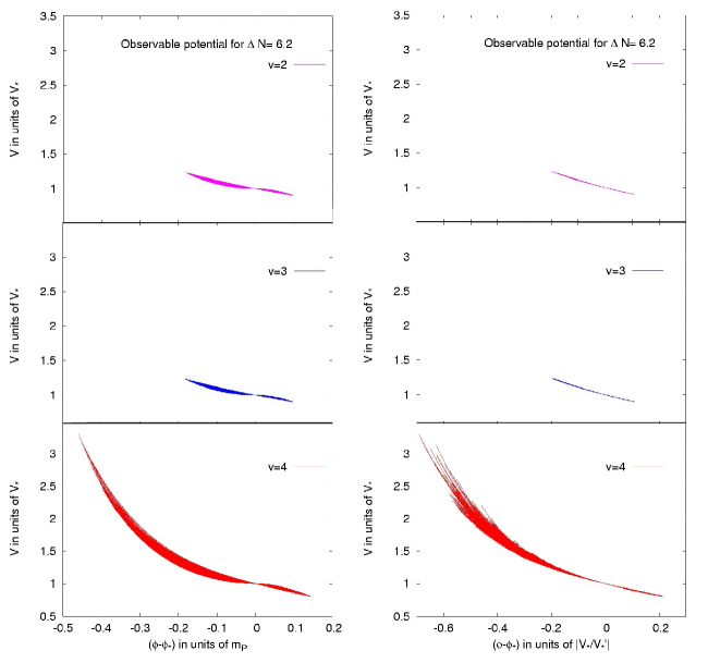
In section II, which contains our main original results, we will fit directly the Taylor-expanded scalar potential of the inflaton to the data. Our reconstructed potentials are displayed in Fig. 1. Unless we impose a “no-running theoretical prior” (i.e., the prejudice that inflation is deep inside the slow-roll regime), our potentials will freely explore the region in parameter space where the running (and eventually the running of the running) are as large as found in section I. So, for self-consistency, we must forget about the slow-roll formalism and compute the exact primordial spectra numerically (as Ref. Martin and Ringeval (2006) did for various specific expressions of the potentials). In a very nice work, Ref. Makarov (2005) gave a few examples of scalar potentials leading to the largest $|\alpha_{S}|$ values allowed by the data, and showed that even in these cases the second-order slow-roll formalism, although inaccurate, remains a reasonable approximation. In the present systematic analysis, which explores the full parameter space of smooth inflationary potentials, we will see that this conclusion does not apply in all cases.

I Fitting the primordial spectrum

Figure 2: Probability distribution of cosmological and inflationary parameters for the models of section I: $p=2$ (green/light solid), $p=3$ (black dashed), and the models of section II: $v=2$ (magenta dot-dashed), $v=3$ (blue dotted), $v=4$ (red/dark solid). For the runs of section I, the free parameters (with flat priors) are the first eight parameters; the corresponding probability for the potential parameters are derived from second-order slow-roll formulae (involving $V_{*}$ to $V^{\prime\prime\prime}_{*}$, so the inferred value of $V^{\prime\prime\prime\prime}_{*}$ remains undetermined). Instead, for the runs of section II, the free parameters are the first five and the last four; the amplitude parameter in the fifth plot is then defined as $\ln\!\left[10^{10}\frac{128\pi V^{3}_{*}}{3V^{\prime 2}_{*}m_{P}^{6}}\right]$; the corresponding $r$, $n_{S}$ and $\alpha_{S}$ are derived from the exact primordial spectra. The data consists of the WMAP 3-year results Spergel et al. (2006); Page et al. (2006); Hinshaw et al. (2006); Jarosik et al. (2006) and the SDSS LRG spectrum Tegmark et al. (2006).

Primordial spectrum parametrization. The usual way of testing inflationary models without making too many assumptions on the inflaton potential is to fit some smooth scalar/tensor primordial spectra, parametrized as a Taylor expansion of $\ln{\cal P}$ with respect to $\ln k$,

$$\ln\frac{{\cal P}_{{\cal R}}(k)}{{\cal P}_{{\cal R}}(k_{*})}=(n_{S}-1)\ln\frac{k}{k_{*}}+\frac{\alpha_{S}}{2}\ln^{2}\frac{k}{k_{*}}+\frac{\beta_{S}}{6}\ln^{3}\frac{k}{k_{*}}...,$$ (2)

and the same holds for ${\cal P}_{h}$ as a function of $n_{T}$, $\alpha_{T}$ and $\beta_{T}$. In single-field inflation, the coefficients of the scalar and tensor spectra are related through the approximate self-consistency relation

$$\frac{d\ln{\cal P}_{h}(k)}{d\ln k}\simeq\frac{1}{8}\frac{{\cal P}_{h}(k)}{{\cal P}_{\cal R}(k)}$$ (3)

which follows trivially from Eq. (1) and becomes exact deep in the slow-roll limit. The sensitivity of current data to gravitational waves is very low, with loose constraints on the shape of ${\cal P}_{h}$. So, even if the slow-roll formalism might become inaccurate in some cases, the data can be fitted assuming that Eq. (3) is exact. In other words, for practical purposes, we can safely use the hierarchy of relations derived from Eq.(3),

$$n_{T}=-r/8,\qquad\alpha_{T}=n_{T}[n_{T}-n_{S}+1],\qquad{\rm etc.},$$ (4)

where $r\equiv{\cal P}_{h}(k_{*})/{\cal P}_{\cal R}(k_{*})$. So, if we decide to Taylor expand the scalar spectrum with $p$ independent coefficients, the total number of free inflationary parameters in the problem is $p$+1, including the tensor-to-scalar amplitude ratio at the pivot scale.

Figure 3: Two-dimensional 68% and 95% confidence level contours based on WMAP 3-year and the SDSS LRG spectrum for the parameters describing the primordial spectra, obtained directly from the MCMC in the case of models $p=2$ (green) and $p=3$ (black), or derived form the exact spectra for models $v=2$ (magenta), $v=3$ (blue), $v=4$ (red).

In principle, $p$ should be chosen according to Occam’s razor: when increasing $p$ does not improve sufficiently the goodness-of-fit, it is time to stop. In a Bayesian analysis, this question is addressed by the computation of the Bayesian evidence Beltran et al. (2005); Trotta (2005); Kunz et al. (2006); Parkinson et al. (2006); Pahud et al. (2006); Liddle et al. (2006); Liddle (2007). However, when the evidence does not vary significantly as a function of $p$, the decision of stopping the expansion remains a personal choice to some extent, and more conservative works should consider higher $p$ values.

The issue of varying $p$ is important in two respects: first, one needs to know how many independent informations the data is providing, i.e., how smooth/complicated the inflaton potential needs to be (for addressing this issue, one could also perform a principal component analysis Leach (2006)); second, it is useful to know whether the bounds on a given cosmological/inflationary parameter $\theta_{i}$ are independent of $p$, or subject to variations when $p$ increases, due to the appearance of new parameter degeneracies.

Results. In order to address these two points, we performed some global parameter fits using the public code cosmomc Lewis and Bridle (2002), with $p$ varying from two (scalar amplitude and tilt) to four (including the tilt running, as well as the running of the running). Our results are summarized in Table 1.

Parameter	$p=2$	$p=3$	$p=4$
$\Omega_{b}h^{2}$	$0.0226\pm 0.001$	$0.022\pm 0.001$	$0.021\pm 0.001$
$\Omega_{cdm}h^{2}$	$0.109\pm 0.004$	$0.109\pm 0.004$	$0.109\pm 0.005$
$\theta$	$1.041\pm 0.004$	$1.040\pm 0.004$	$1.041\pm 0.004$
$\tau$	$0.08\pm 0.01$	$0.10\pm 0.02$	$0.10\pm 0.02$
$\ln[10^{10}{\cal P}_{\cal R}^{k_{*}}]$	$3.08\pm 0.06$	$3.13\pm 0.07$	$3.13\pm 0.07$
$r$	$<0.13$	$<0.3$	$<0.3$
$n_{S}$	$0.97\pm 0.02$	$1.00\pm 0.04$	$1.03\pm 0.05$
$\alpha_{S}$	0	$-0.07\pm 0.04$	$-0.07\pm 0.04$
$\beta_{S}$	0	0	$-0.04\pm 0.04$
$-\ln{\cal L}_{\rm max}$	2688.3	2687.1	2686.5
$E$	1	1.2	1.4

Table 1: Bayesian 68% confidence limits for $\Lambda$CDM inflationary models with $p=2,3,4$ coefficients in the logarithmic Taylor expansion of the scalar primordial spectrum. The last lines show the maximum likelihood value and the Bayesian Evidence (relative to that of $p=2$). The data consists in the WMAP 3-year results Spergel et al. (2006); Page et al. (2006); Hinshaw et al. (2006); Jarosik et al. (2006) and the SDSS-LRG spectrum Tegmark et al. (2006), as implemented in cosmomc Lewis and Bridle (2002).

The relative Bayesian evidence of each model can be easily computed, since the models are nested inside each other Trotta (2005). However, this calculation forces us to choose some explicit Bayesian priors for $\alpha_{S}$ and $\beta_{S}$. Pushing inflation to its limits, we notice that the second slow-roll parameter can in principle vary between plus and minus one, so the scalar tilt could take any value between zero and two. Extreme runnings could be observed in ad-hoc inflationary models such that during the observable e-folds, corresponding to four decades in $k$ space, $n_{S}$ evolves from 0 to 2 or vice-versa. So, the $\alpha_{S}$ prior can be chosen to be a top-hat centered on zero with $\Delta\alpha_{S}=4/\ln(10^{4})\sim 0.4$. Similarly, extreme values of $\beta_{S}$ correspond to $n_{S}$ passing through the sequence 0-2-0 or 2-0-2. This leads to a prior width $\Delta\beta_{S}=16/\ln^{2}(10^{4})\sim 0.2$. With such priors, the Bayesian evidence $E$ increases by a factor

$$\frac{E_{p=3}}{E_{p=2}}=\left[{\cal P}(\alpha_{S}=0)\,\Delta\alpha_{s}\right]^{-1}=[2.1\times 0.4]^{-1}=1.2$$ (5)

when $\alpha_{S}$ is added, and again by

$$\frac{E_{p=4}}{E_{p=3}}=\left[{\cal P}(\beta_{S}=0)\,\Delta\beta_{s}\right]^{-1}=[6.2\times 0.2]^{-1}=1.2$$ (6)

when $\beta_{S}$ is introduced. These numbers are too close to one for drawing definite conclusions: the extra parameters are neither required, neither disfavored by Occam’s Razor.

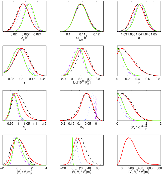
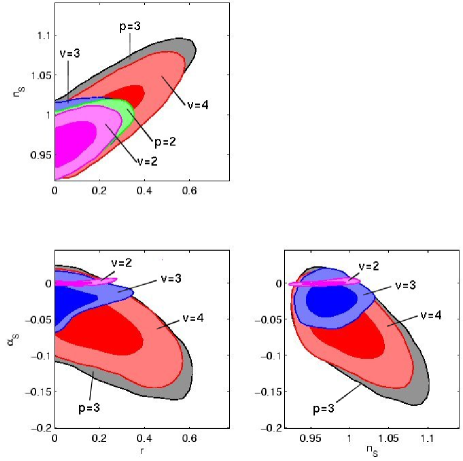
Table 1 shows that adding $\alpha_{S}$ has a small impact on the probability distribution of $\Omega_{b}h^{2}$, $\tau$, $r$, ${\cal P}_{\cal R}(k_{*})$ and $n_{S}$, as found in previous works. However, it is reassuring to note that adding $\beta_{S}$ leave all bounds perfectly stable, except for a small shift to higher $n_{s}$ values. This suggests that including a few higher derivatives beyond $\alpha_{S}$ does not open new parameter degeneracies (this conclusion would probably break if the number of free parameters becomes much larger). Figs. 2, 3 show the likelihood distribution of each parameter as well as some two-dimensional confidence regions for models $p=2$ (green lines) and $p=3$ (black lines).

Impact of small CMB multipoles. The smallest multipoles in the CMB temperature and polarization maps are still controversial. In WMAP data (as well as in previous COBE data), the temperature quadrupoles and octopoles are surprisingly small, while their orientations seem to be correlated (between each other and with the ecliptic plane). Many authors have been investigating possible foregrounds or systematics which could affect these small multipoles (see e.g. Schwarz et al. (2004); Copi et al. (2006, 2007) and references therein). So, it is legitimate to study whether the quadrupole and octopole data have a significant impact on our bounds for the primordial spectrum parameters (a priori, these low temperature multipoles could be partially responsible for the preferred negative value of the tilt).

We repeated the $p=3$ analysis after cutting the temperature and polarization data at $l=2,3$. We found that all probabilities are essentially unchanged, including that for running (the mean value only moves from $-0.67$ to $-0.66$, which is not significant given the precision of the runs). We conclude that our results are independent of the robustness of low mutipole data.

Impact of extra CMB data. There are also discussions about a possible small mismatch in the amplitude of the third acoustic peak probed on the one hand by WMAP, and on the other hand by Boomerang Jones et al. (2006) or other small-scale CMB experiments. We repeated the $p=2$ and $p=3$ analysis including extra data from Boomerang Jones et al. (2006), ACBAR Kuo et al. (2004) and CBI Sievers et al. (2005). The impact on inflationary parameter is found to be very small, although in the $p=3$ case the bound on $r$ gets weaker by 20% and the preferred value of $\alpha_{S}$ goes down by the same amount (i.e., the case for negative running becomes slightly stronger). Other bounds are essentially unchanged. In what follows, we will not include these data sets anymore.

Expectations for the inflaton potential. In the next section, we will directly fit the inflaton potential $V(\phi)$, parametrized as a Taylor expansion near the value $\phi_{*}$ corresponding to Hubble crossing for the pivot scale $k_{*}$. We expect that a global fit with $V(\phi)$ expanded at order $v$ will provide the same qualitative features as the previous power spectrum fit of order $p=v$:

• order $v=2$ ($V^{\prime\prime\prime}=0$) should be sufficient for explaining the data, and will not lead to significant running or deviation from slow-roll. Indeed, the smallness of $r$ and $|n_{S}-1|$ guarantees that the two slow-roll conditions are well satisfied at least near $\phi_{*}$. In addition, with $V^{\prime\prime\prime}=0$, they should remain well satisfied on the edges of the spectrum, and no significant running can be generated.

• order $v\geq 3$ ($V^{\prime\prime\prime\prime}=0$) should not be required by the data, but remains interesting since it will explore the possibility of large running and shift the other parameter distributions as in the previous $p=3$ case. The slow-roll parameters could then become large near the edges, so it is necessary to compute the spectra numerically rather than using any slow-roll approximation.

The results of the next section will confirm this expectation, and prove that order $v=4$ is necessary for exploring the full range of $\alpha_{s}$ probed by the $p=3$ run.

II Fitting the scalar potential

Computing the power spectra numerically. In order to fit directly the inflaton potential, we wrote a new cosmomc module which computes the scalar and tensor primordial spectra exactly, for any given function $V(\phi-\phi_{*})$. This module can be downloaded from the website http://wwwlapp.in2p3.fr/~lesgourgues/inflation/, and easily implemented into cosmomc.

In its present form, our code is not designed for models with very strong deviations from slow-roll. For such extreme models, a given function $V(\phi-\phi_{*})$ would not lead to a unique set of primordial spectra ${\cal P}_{\cal R}(k)$, ${\cal P}_{h}(k)$: the result would depend on the initial conditions in phase space. We decide to limit ourselves to models such that throughout the observable range, the field remains close to the attractor solution for which $\dot{\phi}$ is a unique function $\phi$. In this case, a given function $V(\phi-\phi_{*})$ does lead to unique primordial spectra, and we do not need to introduce an extra parameter $\dot{\phi}_{\rm ini}$. Since the goal of this paper is to test inflationary potentials leading to smooth primordial spectra, this restriction is sufficient. In particular, it enables to explore models for which the running $\alpha_{S}$ is large, deviations from slow-roll are significant, and analytical derivations of the spectra are inaccurate. However, our code cannot deal with the case in which inflation starts just when our observable universe crosses the horizon (for which $\dot{\phi}_{\rm ini}$ would be a crucial extra free parameter).

In cosmomc, we fix once and for all the value of the pivot scale $k_{*}=0.01~{}$Mpc^-1. Then, for each function $V(\phi-\phi_{*})$ passed by cosmomc, our code computes the spectra ${\cal P}_{\cal R}(k)$, ${\cal P}_{h}(k)$ within the range $[k_{\rm min},k_{\rm max}]=[5\times 10^{-6},5]~{}$Mpc^-1 needed by camb, imposing that $aH=k_{*}$ when $\phi=\phi_{*}$. So, the code finds the attractor solution around $\phi=\phi_{*}$, computes $H_{*}$ and normalizes the scale factor so that $a_{*}=k_{*}/H_{*}$. Then, each mode is integrated numerically for $k/aH$ varying between two adjustable ratios: here, $50$ and $1/50$. So, the earliest (resp. latest) time considered in the code is that when $k_{\rm min}/aH=50$ (resp. $k_{\rm max}/aH=1/50$), which in the attractor solution uniquely determines extreme values of $(\phi-\phi_{*})$ according to some potential. In the code this is translated to demanding that $aH$ grows according to the aforementioned ratios: by $50k_{*}/k_{\rm min}$ before $\phi=\phi_{*}$, and by $50k_{\rm max}/k_{*}$ afterwards. Hence, one of the preliminary tasks of the code is to find the earliest time. If by then, a unique attractor solution for the background field cannot be found within a given accuracy (10% for $\dot{\phi}_{\rm ini}$), the model is rejected. So, we implicitly assume that inflation starts at least a few e-folds before the present Hubble scale exits the horizon. In addition, we impose a positive, monotonic potential and an accelerating scale factor during the period of interest. This prescription discards any models with a bump in the inflaton potential or a short disruption of inflation, that could produce sharp features in the power spectra.

As a result of the chosen method, the potential is slightly extrapolated beyond the observable window, in order to reach the mentioned conditions for the beginning and ending of the numerical integration. Although this seems to be in contradiction with the purpose of this paper, i.e. to probe only the observable potential, this extrapolation cannot be avoided if we want to keep the number of free parameters as small as possible. Note that the range of extrapolation is still very small in comparison with an extrapolation over the full duration of inflation after the observable modes have exited the Hubble radius.

In this approach we need not make any assumption about reheating and the duration of the radiation era. As explained in Ref. Ringeval (2007), the evolution during reheating determines the redshift $z_{*}$ at which presently observed perturbations left the Hubble radius during inflation. Probing only the observable window of perturbations, we are allowed to let the subsequent evolution of inflation and reheating, hence the number of e-folds and thereby the redshift $z_{*}$, be unknown.

Parametrization. The inflaton potential is Taylor expanded up to a fixed order, and we let cosmomc probe different values for the derivatives of the inflaton potential at the pivot scale. Since Monte Carlo Markov Chains (MCMC) converge faster if the probed parameters are nearly Gaussian distributed, in fact we recombine to potential parameters in such a way as to probe nearly Gaussian combinations. These combinations are inspired by the slow-roll expression of the spectral parameters (${\cal P}_{\cal R}(k_{*})$, $n_{S}$, $\alpha_{S}$ and $r$) as a function of the potential. We use an amplitude parameter $\frac{128\pi}{3}\frac{V^{3}_{*}}{V^{\prime 2}_{*}m_{P}^{6}}$, which is equal to ${\cal P}_{\cal R}(k_{*})$ at leading order in a slow-roll expansion. The other spectral parameters consist of linear combinations of $(V_{*}^{\prime}/V_{*})^{2}$, $V^{\prime\prime}_{*}/V$, $(V^{\prime\prime\prime}_{*}/V_{*})(V_{*}^{\prime}/V_{*})$ and $(V^{\prime\prime\prime\prime}_{*}/V_{*})(V^{\prime}_{*}/V_{*})^{2}$. Hence it is most likely to find nearly Gaussian shapes for these products in stead of the sole potential derivatives. For the actual expressions for the spectral parameters in terms of the inflaton potential, we refer the reader e.g. to section IV of Leach et al. (2002).

Parameter	$v=2$	$v=3$	$v=4$
$\Omega_{b}h^{2}$	$0.022\pm 0.001$	$0.022\pm 0.001$	$0.022\pm 0.001$
$\Omega_{cdm}h^{2}$	$0.109\pm 0.004$	$0.109\pm 0.004$	$0.109\pm 0.004$
$\theta$	$1.041\pm 0.004$	$1.041\pm 0.004$	$1.040\pm 0.004$
$\tau$	$0.08\pm 0.03$	$0.09\pm 0.03$	$0.10\pm 0.03$
$\ln\!\left[\frac{128\pi 10^{10}V^{3}_{*}}{3V^{\prime 2}_{*}m_{P}^{6}}\right]$	$3.06\pm 0.06$	$3.07\pm 0.06$	$3.11\pm 0.08$
$\left(\frac{V^{\prime}_{*}}{V_{*}}\right)^{2}\!\!\!m_{P}^{2}$	$<0.4$	$<0.4$	$<0.8$
$\frac{V^{\prime\prime}_{*}}{V_{*}}m_{P}^{2}$	$0.1\pm 0.5$	$-0.2\pm 0.6$	$0.4\pm 0.9$
$\frac{V^{\prime\prime\prime}_{*}}{V_{*}}\frac{V^{\prime}_{*}}{V_{*}}m_{P}^{4}$	0	$8\pm 5$	$13\pm 11$
$\frac{V^{\prime\prime\prime\prime}_{*}}{V_{*}}\left(\frac{V^{\prime}_{*}}{V_{*}}\right)^{2}\!\!\!m_{P}^{6}$	0	0	$200\pm 150$
$-\ln{\cal L}_{\rm max}$	2688.3	2687.2	2687.2

Table 2: Bayesian 68% confidence limits for $\Lambda$CDM inflationary models with a Taylor expansion of the inflaton potential at order $v=2,3,4$ (with the primordial spectra computed numerically). The last line shows the maximum likelihood value. The data consists of the WMAP 3-year results Spergel et al. (2006); Page et al. (2006); Hinshaw et al. (2006); Jarosik et al. (2006) and the SDSS LRG spectrum Tegmark et al. (2006), as implemented in cosmomc Lewis and Bridle (2002).

In order to compare the results for the runs with $v=2,3,4$ with those of the previous section, we calculate the spectral parameters of each model numerically. The other way around, we also invert the slow-roll expansion in order to compare the $v=2,3,4$ and $p=2,3$ models in potential-derivative space. Defining $\epsilon_{0}\equiv H(N_{I})/H(N)$ and $\epsilon_{n+1}\equiv\frac{d\ln\left|\epsilon_{n}\right|}{dN}$, where $N=\ln\frac{a}{a_{i}}$ and $H_{i}$ is some initial value of the Hubble factor, the inversion is given by

$$\epsilon_{1} = \frac{r}{16}+\frac{C_{1}}{16}\left(\frac{r^{2}}{8}+(n_{S}-1)r\right)$$ (7)

$$+\mathcal{O}\left(r^{3},\left(n_{S}-1\right)^{3},\alpha_{S}^{3}\right),$$

$$\epsilon_{2} = -(ns-1)+C_{1}\alpha_{S}-\frac{r}{8}-\frac{r}{8}(ns-1)\left(C_{1}-\frac{3}{2}\right)$$ (8)

$$-\left(\frac{r}{8}\right)^{2}(C_{1}-1)+\mathcal{O}\left(r^{3},\left(n_{S}-1\right)^{3},\alpha_{S}^{3}\right),$$

$$\epsilon_{2}\epsilon_{3} = \frac{1}{8}\left(\frac{r^{2}}{8}+(n_{S}-1)r-8\alpha_{S}\right)$$ (9)

$$+\mathcal{O}\left(r^{3},\left(n_{S}-1\right)^{3},\alpha_{S}^{3}\right),$$

where $C_{1}=\gamma_{E}+\ln 2-2\simeq-0.7296$. The value of the potential and its derivatives can be expressed exactly in terms of the slow-roll parameters, which are listed up to the second derivative in Leach et al. (2002). The third derivative reads

$$V^{\prime\prime\prime}=\frac{12m_{p}^{2}H^{2}\sqrt{\pi}}{\sqrt{\epsilon_{1}}}\left(2\epsilon_{1}^{2}-\frac{3\epsilon_{2}\epsilon_{1}}{2}+\frac{\epsilon_{2}\epsilon_{3}}{4}\right).$$ (10)

The fourth derivative of the inflaton potential would be of a higher order in the slow-roll expansion.

Figure 4: Two-dimensional 68% and 95% confidence level contours based on WMAP 3-year and the SDSS LRG spectrum, for the parameters describing the inflaton potential, obtained directly from the MCMC in the case of models $v=2$ (magenta), $v=3$ (blue), $v=4$ (red), or derived from second-order formulas for models $p=2$ (green), $p=3$ (black).

Figure 5: The primordial spectrum for scalar perturbations (left) and tensor perturbations (right) allowed at the 95% C.L. by WMAP 3-year and the SDSS LRG data, for a Taylor expansion of the inflaton potential at order $v=2$ (magenta/light), $v=3$ (blue/dark) or $v=4$ (red/medium). In practice, this plot shows the superposition of 95% of the spectra from our MCMC chains with the best likelihood (after removal of the burn-in phase). All these spectra are computed numerically, rescaled to one at the pivot value $k_{*}$, and displayed in the range which is most constrained by our data set. Note that the shapes of the two spectra are related to each other: so, the tensor spectrum is constrained through that of the scalar spectrum, and not directly by the data, which does not have the required sensitivity.

Figure 6: Precision test of the second-order slow-roll expansion for models allowed at the 95% C.L. by WMAP 3-year and the SDSS LRG data, based on a Taylor expansion of the inflaton potential at order $v=2$ (magenta/light), $v=3$ (blue/dark) or $v=4$ (red/medium). For each model, we plot the spectral parameter $r$ (top left), $n_{S}$ (top right) and $\alpha_{S}$ (bottom left) computed at the pivot scale with two methods: by deriving the primordial spectrum computed numerically (horizontal axis), or with the second-order slow-roll formalism. We checked that the scattering of the point away from the y=x axis reflects inaccuracies in the second-order slow-roll formalism rather than in our code. The bottom right plot shows the inaccuracy in the running as a function of $V^{\prime\prime\prime\prime}_{*}{V^{\prime}}_{*}^{2}/V_{*}^{3}$ for the $v=4$ model.

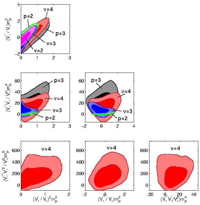
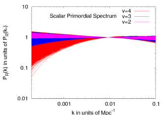
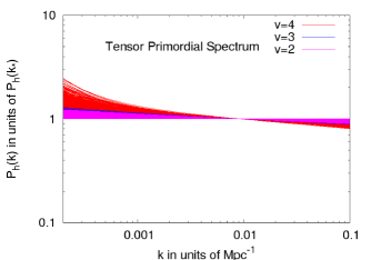
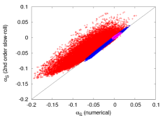
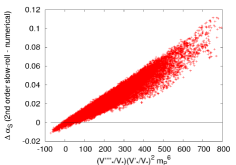
Results. The allowed ranges, parameter likelihoods and two-dimensional contours from all our runs are summarized respectively in Table 2, Fig. 2 and Figs. 3, 4. The allowed shape of primordial scalar and tensor spectra is shown in Figs. 5.

First we ran a chain for the model at order $v=2$. As expected, the results confirm those obtained fitting the spectral parameters up to order $p=2$, which can be seen in Figs. 2 and 4 and the upper left chart in Fig. 3, by comparing the magenta and green lines. This can be translated into the statement that fixing the running of the tilt to zero is almost equivalent to fixing third and higher derivatives of the potential to zero. The resulting bounds can be read from Table 2, and the correlation between $V^{\prime}_{*}/V_{*}$ and $V^{\prime\prime}_{*}/V_{*}$ is well accounted by the relation

$$m_{P}^{2}\left[2.2\left(\frac{V^{\prime}_{*}}{V_{*}}\right)^{2}-\frac{V^{\prime\prime}_{*}}{V_{*}}\right]=0.6\pm 0.2~{}.\qquad(68\%{\rm C.L.})$$ (11)

Note that the numerically calculated running in the models with $v=2$ is not strictly zero but allows a very small region of nonzero running. Similarly, the derived bounds from the models with $p=2$ on the potential parameters allow for very small regions of nonzero second and third derivative. This merely reflects the expansions in different parameterizations than an indication for running (or nonzero higher derivatives of the potential).

Including a third derivative does allow for models to have a more significant running, which is clearly visible Fig. 5. Yet, as seen in Figs. 2, 3 and 4, the models with $v=3$ (blue line) do not explore the full range of parameters which is indicated by the models with $p=3$ (black line), in particular for $\alpha_{S}$, and do not show as much a sign of degeneracy between $V^{\prime\prime\prime}_{*}V^{\prime}_{*}/V_{*}^{2}$ and $V_{*}^{\prime 2}$ as the derived potential derivatives from the models with $p=3$, in Fig. 4. The relation between $V^{\prime\prime}$ and $V^{\prime 2}$ remains almost unchanged. Inversely, in Fig. 3 we see the same effect in spectral parameter space.

The remaining discrepancy between models $v=3$ and $p=3$ led us to including the fourth derivative of the inflaton potential as a free parameter, i.e. $v=4$. The resulting power spectra, shown in Fig. 5, show a larger negative running than in the $v=3$ case, even with significant running of the running on the largest scales. In Fig. 2 we see that the model $v=4$ (red line) does probe the same range of runnings of the tilt as allowed in the model $p=3$. Looking at two-dimensional projections, we see that the $p=3$ and $v=4$ contours are closer to each other in spectral parameter space (Fig. 3) than in potential parameter space (Fig. 4): this reflects the inaccuracy of second-order slow-roll expressions, as explained in the next paragraph. In the model $v=4$ the range for the lower derivatives of the potential is slightly larger than in the models with $v<4$, which has its repercussions embodied in slight degeneracies between the fourth derivative and the lower derivatives.

Note that all figures containing information on the fourth derivative of the potential contain only the model $v=4$ (red line) and not those with $p=2$ or $p=3$, since in the slow-roll approximation one would need to go to third order in order to infer $V^{\prime\prime\prime\prime}_{*}$ from the primordial spectrum.

Finally, it is worth pointing out that the results at all orders in both parameterizations still allow for a flat (Harrison-Zel’dovich) spectrum at the 95% C.L., or for a linear potential at the 68% C.L.

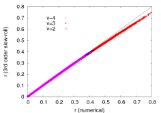
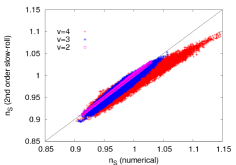
Precision of the slow-roll approximation. In Fig. 6 we show the discrepancy between the numerical results for the spectral parameters (top left: $r$, top right: $n_{S}$, bottom left: $\alpha_{S}$) and those obtained using the slow-roll approximation up to third order in the derivatives of the inflaton potential (second order in slow-roll parameters for $n_{S}$ and $\alpha_{S}$, third order for $r$). The numerically calculated parameters can in this context be treated as exact, since they do not involve any approximation (within first-order cosmological perturbation theory), and remain perfectly stable when we increase the precision parameters of our code. As $r$ naturally comes out at one order higher in the slow-roll expansion than $n_{S}$ and $\alpha_{S}$, the top left plot ($r$) shows less discrepancy than do the plots for $n_{S}$ and $\alpha_{S}$. However, for large $r$ there is a clear deviation from slow-roll in the results with $v=4$ (red), up to $\sim$7%. In the plot for $n_{S}$ it is clearly seen that second order slow roll is only accurate up to $\sim 3\%$ for the run with $v=3$ (blue region). This discrepancy is important, since the data constrains $n_{S}$ with a standard deviation $\sigma\sim 2$%. When a fourth derivative of the inflaton potential is included, second-order slow roll becomes really inaccurate, with a typical error of 10% on $n_{S}$, while the running can be wrongfully estimated by as much as $\Delta\alpha_{S}=0.1$, i.e. three standard deviations given the current data. In a future work, it would therefore be useful to compute the next-order contributions to the running analytically (the bottom right diagram shows the quasi-linear dependence of $\alpha_{S}$ on the combination $V^{\prime\prime\prime\prime}_{*}{V^{\prime}}_{*}^{2}/V_{*}^{3}$).

III Conclusions

In this work, we derived some constraints on the inflaton potential from up-to-date CMB and LSS data. Our CMB data consists in the WMAP 3-year measurement of the temperature and polarization power spectrum. We did include the first (controversial) multipoles, after checking in section I that they do not have a significant impact on the determination of the primordial spectrum tilt and running. Our analysis differs from previous works for several reasons. First, we directly fit the parameters describing the inflaton potential, instead of constraining first the primordial spectra, and reconstructing the inflaton potential afterwards. Second, we Taylor-expand the inflaton potential in the vicinity of the pivot scale at a rather high order (up to $v=4$), and see that such a high order is important e.g. for exploring all the parameter space allowed by the data in terms of running of the scalar spectrum tilt. Third, we compute the scalar and tensor spectra for each model numerically, and find that for the models considered here this is important, since the spectra derived from the second-order slow-roll formalism are inaccurate by the same order as the observational constraints themselves.

However, the most important peculiarity of this work is our choice to focus only on the observable region of the inflaton potential, not making any assumption on the shape of the potential between the observable region and the minimum close to which inflaton stops after approximately 50 e-folds (depending on the scale of inflation). This choice has a crucial impact on the results. If we did extrapolate the inflaton potential over 50 e-folds, keeping the same order in the Taylor expansion, our models would be more severely constrained, since the requirement of 50 extra e-folds would kill many of the allowed potentials presented here. We are perfectly aware of this, and wish to point out that this is one of two points of view, which are both equally sensible.

From one point of view, if one works under the prejudice that the inflaton potential should not be too complicated, then it is extremely relevant to consider the global shape of the potential and to throw away all models which cannot sustain 60 inflationary e-folds. Many papers use this approach, using sometimes Monte Carlo methods in which the potential (or the Hubble flow $H(N)$) is Taylor expanded over the 60 e-folds at high order.

From another point of view, if one wants to address the question of what is strictly allowed by the data, then even a high-order Taylor expansion of the full potential sounds unsatisfactory for modeling all its possible variations during such a long history as 60 e-folds (especially if one keeps in mind that some other fields could then play a role: triggering a phase transition, inducing complicated shapes as in the string-inspired landscape scenarios, etc.). On the contrary, in this philosophy, one should only try to parametrize the inflaton potential in the range probed by cosmological data, i.e. around six or seven e-folds. This is what we did here, with a Taylor expansion up to fourth order.

The two approaches lead, of course, to radically different conclusions. For instance, in the first method, one would conclude that during the observational e-folds the inflaton must be deep in the slow-roll regime, since it is necessary to sustain a number of e-folds which is an order of magnitude higher. The running would then be very constrained Easther and Peiris (2006). In the second method, it is not a problem to satisfy slow-roll only marginally on the edges of the observable range. Even if $\epsilon_{1}$ grows dangerously close to one when cluster scales exit the Hubble radius, the potential could become much flatter afterwards, and sustain any desired amount of inflation.

Our main results for the inflaton potential reconstruction are summarized in Figs. 1, 2, 4 and Table 2. We also showed up to what extent the slow-roll formalism reveals to be inaccurate in the current context in Fig. 6. This motivates possible future works concerning the next-order slow-roll expressions.

Following the same approach, this work could be improved by adding more large-scale structure data e.g. from Lyman-$\alpha$ forests or weak lensing, which have a good power for further constraining the primordial spectrum on smaller scales than the SDSS LRG data. Here we choose to use a very restricted data set, in order to derive rather conservative and robust results.

More generally, we point out that our cosmomc module for computing the primordial spectra numerically can be used in different contexts, within cosmomc or separately, and even (after minor modifications) for studying more complicated models producing characteristic features in the primordial spectra. The module was written in a user-friendly way and made publicly available on the website http://wwwlapp.in2p3.fr/~lesgourgues/inflation/.

References

- Starobinsky (1980) A. A. Starobinsky, Phys. Lett. B91, 99 (1980).
- Guth (1981) A. H. Guth, Phys. Rev. D23, 347 (1981).
- Sato (1981) K. Sato, Mon. Not. Roy. Astron. Soc. 195, 467 (1981).
- Hawking and Moss (1982) S. W. Hawking and I. G. Moss, Phys. Lett. B110, 35 (1982).
- Linde (1982a) A. D. Linde, Phys. Lett. B108, 389 (1982a).
- Linde (1983) A. D. Linde, Phys. Lett. B129, 177 (1983).
- Starobinsky (1979) A. A. Starobinsky, JETP Lett. 30, 682 (1979).
- Hawking (1982) S. W. Hawking, Phys. Lett. B115, 295 (1982).
- Starobinsky (1982) A. A. Starobinsky, Phys. Lett. B117, 175 (1982).
- Guth and Pi (1982) A. H. Guth and S. Y. Pi, Phys. Rev. Lett. 49, 1110 (1982).
- Linde (1982b) A. D. Linde, Phys. Lett. B116, 335 (1982b).
- Bardeen et al. (1983) J. M. Bardeen, P. J. Steinhardt, and M. S. Turner, Phys. Rev. D28, 679 (1983).
- Abbott and Wise (1984) L. F. Abbott and M. B. Wise, Nucl. Phys. B244, 541 (1984).
- Salopek et al. (1989) D. S. Salopek, J. R. Bond, and J. M. Bardeen, Phys. Rev. D40, 1753 (1989).
- Spergel et al. (2006) D. N. Spergel et al. (2006), eprint astro-ph/0603449.
- Page et al. (2006) L. Page et al. (2006), eprint astro-ph/0603450.
- Hinshaw et al. (2006) G. Hinshaw et al. (2006), eprint astro-ph/0603451.
- Jarosik et al. (2006) N. Jarosik et al. (2006), eprint astro-ph/0603452.
- Linde (1991) A. D. Linde, Phys. Lett. B259, 38 (1991).
- Linde (1994) A. D. Linde, Phys. Rev. D49, 748 (1994), eprint astro-ph/9307002.
- Copeland et al. (1994) E. J. Copeland, A. R. Liddle, D. H. Lyth, E. D. Stewart, and D. Wands, Phys. Rev. D49, 6410 (1994), eprint astro-ph/9401011.
- Peiris and Easther (2006a) H. Peiris and R. Easther, JCAP 0607, 002 (2006a), eprint astro-ph/0603587.
- de Vega and Sanchez (2006) H. J. de Vega and N. G. Sanchez (2006), eprint astro-ph/0604136.
- Easther and Peiris (2006) R. Easther and H. Peiris, JCAP 0609, 010 (2006), eprint astro-ph/0604214.
- Kinney et al. (2006) W. H. Kinney, E. W. Kolb, A. Melchiorri, and A. Riotto, Phys. Rev. D74, 023502 (2006), eprint astro-ph/0605338.
- Martin and Ringeval (2006) J. Martin and C. Ringeval, JCAP 0608, 009 (2006), eprint astro-ph/0605367.
- Covi et al. (2006) L. Covi, J. Hamann, A. Melchiorri, A. Slosar, and I. Sorbera, Phys. Rev. D74, 083509 (2006), eprint astro-ph/0606452.
- Finelli et al. (2006) F. Finelli, M. Rianna, and N. Mandolesi, JCAP 0612, 006 (2006), eprint astro-ph/0608277.
- Peiris and Easther (2006b) H. Peiris and R. Easther, JCAP 0610, 017 (2006b), eprint astro-ph/0609003.
- Destri et al. (2007) C. Destri, H. J. de Vega, and N. G. Sanchez (2007), eprint astro-ph/0703417.
- Ringeval (2007) C. Ringeval (2007), eprint astro-ph/0703486.
- Cardoso (2007) A. Cardoso, Phys. Rev. D75, 027302 (2007), eprint astro-ph/0610074.
- Cline and Hoi (2006) J. M. Cline and L. Hoi, JCAP 0606, 007 (2006), eprint astro-ph/0603403.
- Grivell and Liddle (2000) I. J. Grivell and A. R. Liddle, Phys. Rev. D61, 081301 (2000), eprint astro-ph/9906327.
- Steinhardt and Turner (1984) P. J. Steinhardt and M. S. Turner, Phys. Rev. D29, 2162 (1984).
- Salopek and Bond (1990) D. S. Salopek and J. R. Bond, Phys. Rev. D42, 3936 (1990).
- Liddle et al. (1994) A. R. Liddle, P. Parsons, and J. D. Barrow, Phys. Rev. D50, 7222 (1994), eprint astro-ph/9408015.
- Stewart and Lyth (1993) E. D. Stewart and D. H. Lyth, Phys. Lett. B302, 171 (1993), eprint gr-qc/9302019.
- Lidsey et al. (1997) J. E. Lidsey et al., Rev. Mod. Phys. 69, 373 (1997), eprint astro-ph/9508078.
- Gong and Stewart (2001) J.-O. Gong and E. D. Stewart, Phys. Lett. B510, 1 (2001), eprint astro-ph/0101225.
- Dodelson and Stewart (2002) S. Dodelson and E. Stewart, Phys. Rev. D65, 101301 (2002), eprint astro-ph/0109354.
- Schwarz et al. (2001) D. J. Schwarz, C. A. Terrero-Escalante, and A. A. Garcia, Phys. Lett. B517, 243 (2001), eprint astro-ph/0106020.
- Stewart (2002) E. D. Stewart, Phys. Rev. D65, 103508 (2002), eprint astro-ph/0110322.
- Leach et al. (2002) S. M. Leach, A. R. Liddle, J. Martin, and D. J. Schwarz, Phys. Rev. D66, 023515 (2002), eprint astro-ph/0202094.
- Hansen and Kunz (2002) S. H. Hansen and M. Kunz, Mon. Not. Roy. Astron. Soc. 336, 1007 (2002), eprint hep-ph/0109252.
- Caprini et al. (2003) C. Caprini, S. H. Hansen, and M. Kunz, Mon. Not. Roy. Astron. Soc. 339, 212 (2003), eprint hep-ph/0210095.
- Liddle (2003) A. R. Liddle, Phys. Rev. D68, 103504 (2003), eprint astro-ph/0307286.
- Choe et al. (2004) J. Choe, J.-O. Gong, and E. D. Stewart, JCAP 0407, 012 (2004), eprint hep-ph/0405155.
- Habib et al. (2005) S. Habib, A. Heinen, K. Heitmann, and G. Jungman, Phys. Rev. D71, 043518 (2005), eprint astro-ph/0501130.
- Joy et al. (2005) M. Joy, E. D. Stewart, J.-O. Gong, and H.-C. Lee, JCAP 0504, 012 (2005), eprint astro-ph/0501659.
- Kadota et al. (2005) K. Kadota, S. Dodelson, W. Hu, and E. D. Stewart, Phys. Rev. D72, 023510 (2005), eprint astro-ph/0505158.
- Casadio et al. (2006) R. Casadio, F. Finelli, A. Kamenshchik, M. Luzzi, and G. Venturi, JCAP 0604, 011 (2006), eprint gr-qc/0603026.
- de Oliveira and Terrero-Escalante (2006) H. P. de Oliveira and C. A. Terrero-Escalante, JCAP 0601, 024 (2006), eprint astro-ph/0511660.
- Makarov (2005) A. Makarov, Phys. Rev. D72, 083517 (2005), eprint astro-ph/0506326.
- Tegmark et al. (2006) M. Tegmark et al., Phys. Rev. D74, 123507 (2006), eprint astro-ph/0608632.
- Beltran et al. (2005) M. Beltran, J. Garcia-Bellido, J. Lesgourgues, A. R. Liddle, and A. Slosar, Phys. Rev. D71, 063532 (2005), eprint astro-ph/0501477.
- Trotta (2005) R. Trotta (2005), eprint astro-ph/0504022.
- Kunz et al. (2006) M. Kunz, R. Trotta, and D. Parkinson, Phys. Rev. D74, 023503 (2006), eprint astro-ph/0602378.
- Parkinson et al. (2006) D. Parkinson, P. Mukherjee, and A. R. Liddle, Phys. Rev. D73, 123523 (2006), eprint astro-ph/0605003.
- Pahud et al. (2006) C. Pahud, A. R. Liddle, P. Mukherjee, and D. Parkinson, Phys. Rev. D73, 123524 (2006), eprint astro-ph/0605004.
- Liddle et al. (2006) A. R. Liddle, P. Mukherjee, and D. Parkinson, Astron. Geophys. 47, 4.30 (2006), eprint astro-ph/0608184.
- Liddle (2007) A. R. Liddle (2007), eprint astro-ph/0701113.
- Leach (2006) S. Leach, Mon. Not. Roy. Astron. Soc. 372, 646 (2006), eprint astro-ph/0506390.
- Lewis and Bridle (2002) A. Lewis and S. Bridle, Phys. Rev. D66, 103511 (2002), eprint astro-ph/0205436.
- Schwarz et al. (2004) D. J. Schwarz, G. D. Starkman, D. Huterer, and C. J. Copi, Phys. Rev. Lett. 93, 221301 (2004), eprint astro-ph/0403353.
- Copi et al. (2006) C. J. Copi, D. Huterer, D. J. Schwarz, and G. D. Starkman, Mon. Not. Roy. Astron. Soc. 367, 79 (2006), eprint astro-ph/0508047.
- Copi et al. (2007) C. Copi, D. Huterer, D. Schwarz, and G. Starkman, Phys. Rev. D75, 023507 (2007), eprint astro-ph/0605135.
- Jones et al. (2006) W. C. Jones et al., Astrophys. J. 647, 823 (2006), eprint astro-ph/0507494.
- Kuo et al. (2004) C.-l. Kuo et al. (ACBAR), Astrophys. J. 600, 32 (2004), eprint astro-ph/0212289.
- Sievers et al. (2005) J. L. Sievers et al. (2005), eprint astro-ph/0509203.