Eppur Si Muove:
On The Motion of the Acoustic Peak in the Correlation Function

Abstract

The baryonic acoustic signature in the large-scale clustering pattern of galaxies has been detected in the two-point correlation function. Its precise spatial scale has been forwarded as a rigid-rod ruler test for the space-time geometry, and hence as a probe for tracking the evolution of Dark Energy. Percent-level shifts in the measured position can bias such a test and erode its power to constrain cosmology. This paper addresses some of the systematic effects that might induce shifts: namely non-linear corrections from matter evolution, redshift space distortions and biasing. We tackle these questions through analytic methods and through a large battery of numerical simulations, with total volume of the order $\sim 100~{}[{\rm Gpc}^{3}\,h^{-3}]$. A toy-model calculation shows that if the non-linear corrections simply smooth the acoustic peak, then this gives rise to an ‘apparent’ shifting to smaller scales. However if tilts in the broad band power spectrum are induced then this gives rise to more pernicious ‘physical’ shifts. Our numerical simulations show evidence of both: in real space and at z=0, for the dark matter we find percent level shifts; for haloes the shifts depend on halo mass, with larger shifts being found for the most biased samples, up to $3\%$. From our analysis we find that physical shifts are greater than $\sim 0.4\%$ at $z=0$. In redshift space these effects are exacerbated, but at higher redshifts are alleviated. We develop an analytical model to understand this, based on solutions to the pair conservation equation using characteristic curves. When combined with modeling of pairwise velocities the model reproduces the main trends found in the data. The model may also help to unbias the acoustic peak.

I Introduction

Within the last few years the discipline of physical cosmology has greatly benefited from a considerable influx of extremely high fidelity data-sets, which have enabled measurements of the large scale structure of the Universe to be made with unprecedented precision; and together these data have led to the establishment of the ‘standard model of cosmology’: the flat, Dark Energy dominated collisionless Cold Dark Matter (CDM) model Spergel et al. (2006); Tegmark et al. (2006); S nchez et al. (2006); Astier et al. (2006); Hoekstra et al. (2006); Cole et al. (2005); Eisenstein et al. (2005). Whilst the CDM particles are well founded from a particle physics point of view, the Dark Energy may arise through a number of possible mechanisms, most of which are of deep consequence to much of physics if found to be true Peebles & Ratra (2003); DETF (2006); ESO (2006). The task of modern theoretical and observational cosmology, therefore, is to construct robust tests to expose the true physical character of the Dark Energy and hence differentiate between hypotheses. A number of experiments are currently underway with this sole purpose in view, and many more are being planned for the future (see DETF (2006); ESO (2006) and references there in for a comprehensive review of current and future missions). The Dark Energy tests fall into two main classes: those which perform geometric tests of gravity and those which perform growth of structure tests. The geometric tests are essentially the use of ‘standard candles’ (Type Ia Supernova) and ‘standard rods’ (baryonic acoustic oscillations), whereas the growth of structure tests, examine how the growth rate of perturbations changes as a function of cosmological epoch. Weak lensing by large scale structure and the multiplicity function of clusters fall into both categories and therefore potentially offer the most powerful discriminatory means. However, in order to make precise, accurate and useful constraints on the Dark Energy, the systematics of each experiment must be fully understood and controlled to sub-percent accuracy DETF (2006); ESO (2006) – the removal of ‘unknown unknowns’ is imperative.

For instance, the standard candle measurement from Type Ia supernovae must address the issue of whether or not the ensemble of candles evolves with redshift, i.e. through metalicity effects, or evolution of the underlying host galaxy properties as a function of redshift. Moreover until the ‘true’ mechanism that drives the nova is understood, it may be the case that this potential systematic can only be quantified and eliminated once the data are in hand.

In this paper we shall restrict our attention to the second of the geometric tests, that is the standard rod measurement from the Baryonic Acoustic Oscillations (BAO). Like the standard candle test, this method also suffers from potential systematics; the three knowns in this case are: nonlinear mass evolution, non-linear bias and redshift space distortions (hereafter, we shall refer to these together as clustering systematics). However, unlike the case for Type Ia Supernova, because the processes driving any possible evolution are plausibly understandable ab-initio, there is not much room for unknown unknowns and there is some hope for estimating and mitigating these effects well-before the data streams in from the next generation surveys. This is important because if the BAO peak is displaced by even 1%, this will induce a bias in the inferred value of the dark energy parameter $w$ on the order of $~{}5\%$ Eisenstein et al. (2005); Angulo et al. (2007).

The physical picture for the BAO signature is as follows: before the epoch of recombination, acoustic oscillations were able to propagate through the photon-baryon plasma at the sound speed, and these waves were weakly coupled to dark matter through gravity. After recombination the photons free stream out of the perturbations and this gives rise to the observed CMB (Hinshaw et al. (2006)), the dark matter and segregated baryons then relax together over time and the self-same acoustic features that are imprinted in the CMB become imprinted in the dark matter distribution. The characteristic scale for the acoustic waves is set by the sound horizon at last scattering $r_{*}$ (see Eisenstein & Hu (1998) for a description of how to calculate this), and this in turn imprints a characteristic scale in the pattern of galaxies and it is supposed that this has the properties of a ‘standard rod’.

The BAO features have been detected by various groups: in the two-point correlation function of Luminous Red Galaxies (LRG) by Eisenstein et al. (2005), and in the power spectrum of galaxies and LRGs by Percival et al. (2001); Tegmark et al. (2004); Cole et al. (2005); Hutsi (2006a, b); Tegmark et al. (2006); Padmanabhan et al. (2006); Percival et al. (2007a, b). The BAOs have also been the subject of much vigorous theoretical and numerical research Meiskin, White & Peacock (1999); Blake & Glazebrook (2003); Seo & Eisenstein (2005); White (2005); Angulo et al. (2005); Springel et al. (2005); Dolney, Jain & Takada (2006); Bernstein (2006); Huff et al. (2006); Eisenstein, Seo & White (2006); Eisenstein et al. (2006); Jeong & Komatsu (2006); Wang (2006); Smith, Scoccimarro & Sheth (2007); Ma (2007); Angulo et al. (2007); Crocce & Scoccimarro (2007); Matarrese & Pietroni (2007). The question of whether there are non-linear effects at play on the acoustic scale, is not an open question Meiskin, White & Peacock (1999), however, whether these non-linearities give rise to an actual motion of the acoustic peak – apparent or physical – is of great debate, and the most recent literature concerned with this question reaches conflicting conclusions: Guzik, Bernstein & Smith (2007) used the fitting formula for the power spectrum from Smith et al. (2003) to conclude that, there is a shift due to nonlinear mass evolution on the order of $\sim 2\%$ at $z=0$. Seo & Eisenstein (2005) used numerical simulations to show that there were changes to the broad band power spectra of dark matter and haloes, and in both real and redshift space, however they argued that provided these were accounted for, no overall shift in the acoustic peak position would be induced. Smith, Scoccimarro & Sheth (2007) used numerical simulations with improved resolution to convincingly confirm the results from Seo & Eisenstein (2005), that the power spectra were not immune to strong broad band tilts. Based on these results they suggested that percent level shifts in the position of the acoustic peak were highly plausible. The main findings of these works were most recently substantiated by Angulo et al. (2007). On the other hand, Eisenstein, Seo & White (2006) used a model based on Lagrangian displacements of the initial density distribution to argue that any acoustic peak shift in the dark matter should be only of the order $10^{-4}$ at $z=0$, although they do note that “galaxy bias could produce a sub-percent shift”. In addition, Ma (2007) studied how a relatively (by BAO standards) large peak in the initial power spectrum evolved in numerical simulations and concluded that there were no noticeable shifts, in agreement with Eisenstein, Seo & White (2006).

In what follows, we examine this issue in detail. We do this in a two-fold way: Firstly, we generate a large ensemble of large volume numerical simulations to quantify the possible effects. Secondly, we develop a new analytical model, which is based on a new solution for the pairwise conservation of particle pairs. When combined with a careful modeling of the divergence of pairwise velocities beyond linear theory this method is shown to capture the main effects that are found in the the simulations.

The subject of this paper is therefore to answer the following important questions: Does non-linear evolution generate a displacement of the peak of the correlation function? If so does the observed shift depend on the halo/galaxy sample considered and how? Recently, there has been a number of different approaches to estimating the sound horizon from observational data, however, so far as we know, it has not been shown that any of these estimators are consistent, unbiased, or indeed minimum variance estimators. The results presented in this work and from our previous study of the power spectrum Smith, Scoccimarro & Sheth (2007); Crocce & Scoccimarro (2007) should act as an important empirical guide for constructing such quantities.

The paper is structured as follows: In Section II we discuss a toy model that shows that an effective smoothing of the acoustic peak in the two-point function leads to an ‘apparent’ motion of the peak. Here we also show how if nonlinear evolution induces a broad band tilt in the underlying linear power spectrum, further shifts in the peak position are to be expected – these we shall class as ‘physical’ shifts. Then in Section III we describe our ensemble of numerical simulations and present our measurements for the two-point correlation function of dark matter and haloes in real and redshift space, including a detailed analysis of our data. In Section IV we describe our new physical model and demonstrate how it gives rise to a transformation of the structure of the peak in the dark matter and halo correlation functions – and that this gives rise to a physical motion of the peak. We also compare our analytic model with the results from the numerical simulation and show that they are in close agreement. Finally, Section V summarizes our results, and discusses them in the wider context.

II Apparent and physical shifts

II.1 Motivation

Motivated by the calculation of the real space dark matter correlation function in renormalized perturbation theory (hereafter, RPT) Crocce & Scoccimarro (2006a, b), we can write the observed correlation function in terms of the linear one through the following relation:

$$\xi_{\rm obs}(r)\approx\int\xi_{{\rm lin}}(r-r^{\prime})\,K(r^{\prime})\,d^{3}r^{\prime}+\xi_{\rm mc}(r)\ ,$$ (1)

where the first term on the left-hand-side represents the linear correlation function convolved with some symmetric kernel, $K(r)$, and the second term, $\xi_{\rm mc}$, describes any effects due to non-linear mode-coupling. The distinction between these two terms may be more clearly seen in Fourier space: the first term is directly proportional to the linear power spectrum at the same scale, and the second term represents a weighted sum over the information from different neighboring wavemodes. Note that such decomposition can always be made. In RPT, the kernel $K$ is well approximated by a Gaussian Crocce & Scoccimarro (2006b), a result that becomes exact in the Zel’dovich approximation Bharadwaj (1996); Crocce & Scoccimarro (2006b); Eisenstein, Seo & White (2006).

Setting aside $\xi_{\rm mc}$ for the moment, we remark that it is sometimes thought that convolution with a Gaussian does not lead to a shift in the BAO peak position. In the following sub-section we will show explicitly that this is not correct and that the convolution with a symmetric filter does shift the peak, and that this is solely due to the fact that $\xi_{{\rm lin}}$ is not symmetric about the acoustic peak. However, as we mention in the following sub-section this apparent shifting of the peak may be corrected for.

Returning now to the issue of mode coupling, as we will show in this work through our numerical simulations and through our theoretical analysis, the term $\xi_{{\rm mc}}$ in Eq. (1) gives rise to an actual ‘physical’ shift towards smaller scales as the clustering evolves. For reasons which are now clear, we shall now refer to the shifts that are generated by the first term as being apparent, and those due to the second, as being physical. In the next subsection we present a toy-model to further illustrate the meaning of these terms.

Figure 1: Halo correlation functions at $z=0$ in real (top) and redshift (bottom) space. Different symbols in each panel show results for massive (top) to less massive halos (bottom). Table 1 gives the precise bins in halo mass. Error bars come from the dispersion between the measured $\xi$ in our 50 simulations; a total volume of $105\,(\!\,h^{-1}\,{\rm Gpc})^{3}$. Solid line in top panel shows the linear theory correlation function multiplied by an arbitrary constant so that it approximately matches the signal from the intermediate mass bin. Vertical dashed line shows the position of the acoustic peak in this linear correlation function: it lies at $106\,h^{-1}\,{\rm Mpc}$.

Figure 2: Same as Fig. 1 but at $z=0.5$.

Figure 3: Same as Fig. 1 but at $z=1$.

II.2 A toy model for the shifts

Part of the following analysis was inspired by ideas first presented by Guzik, Bernstein & Smith (2007). In that work one of the issues addressed was the apparent shift of the acoustic peak position, induced by an inhomogeneous selection function. Here we use similar arguments, but directly connected to the distortions induced by the non-linear clustering transformation and bias, to examine the apparent shifts. Those familiar with the analysis of Guzik, Bernstein & Smith (2007) may wish to jump directly to Eq. (7), which should be familiar.

To begin our toy-model, let us suppose that the linear theory correlation function can be well approximated by a power-law plus a Gaussian bump with peak position located at $r_{p}$:

$$\xi(r)=A_{p}\left(r_{p}\over r\right)^{\gamma}+A_{G}\,\exp\Bigl{[}-\frac{(r-r_{p})^{2}}{2\sigma^{2}}\Bigr{]}\ .$$ (2)

This is a reasonable approximation, since the transfer function can be decomposed into a smooth component, which models the suppression of dark matter fluctuations due to radiation dominated growth and baryon drag effects, and an oscillatory piece that comes from the baryons clumped around the sound horizon: i.e. $T(k)\equiv T_{\rm smooth}(k)+T_{\rm BAO}(k)$ (see Eisenstein & Hu (1998)); on squaring and Fourier transforming we get $\xi(r)\equiv\xi_{\rm smooth}(r)+\xi_{\rm BAO}(r)$, where we have for simplicity neglected the cross-terms from $T^{2}(k)$ (this is a toy-model). Restricting the range of interest to be small enough so that $\xi_{\rm smooth}(r)$ is close to a power-law, then we would have something like our Eq. (2).

The presence of the power-law means that the location of the local maximum, say $r_{\rm max}$, will differ from $r_{p}$. Requiring $d\xi/dr=0$ means

$$A_{p}\,\gamma\left({r_{p}\over r_{m}}\right)^{\gamma+1}=\left(1-{r_{m}\over r_{p}}\right)\,{r_{p}^{2}\over\sigma^{2}}\,G(r_{m})\ .$$ (3)

If $r_{m}=r_{p}(1-\epsilon)$ then

$$A_{p}\,\gamma\,(1-\epsilon)^{-\gamma-1}=\epsilon\,{r_{p}^{2}\over\sigma^{2}}\,G(r_{m})\ .$$ (4)

If $(r_{p}-r_{m})^{2}\equiv\epsilon^{2}r_{p}^{2}\ll\sigma^{2}$ (meaning the offset from $r_{p}$ is small compared to the width of the bump), then this becomes

$$A_{p}\,\gamma\,(1-\epsilon)^{-\gamma-1}=\epsilon\,{r_{p}^{2}\over\sigma^{2}}\,A_{G}\,\left[1-{\epsilon^{2}r_{p}^{2}\over 2\sigma^{2}}\right]\ .$$ (5)

To first order in $\epsilon$, this is

$$\epsilon=\left[{A_{G}/A_{p}\over\gamma\,(\sigma^{2}/r_{p}^{2})}-(1+\gamma)\right]^{-1}.$$ (6)

The fact that we call it a bump means that $A_{G}>A_{p}$. In addition, we are interested in the case where $\sigma\ll r_{p}$, thus our final expression for the peak in the linear correlation function is

$$\epsilon_{\rm lin}\approx\gamma\,\left({\sigma\over r_{p}}\right)^{2}\,\left({A_{p}\over A_{G}}\right).$$ (7)

This shows that the fractional shift from $r_{p}$ is large if $\gamma$ is large (meaning the amplitude of the power law component is changing rapidly), or if $\sigma/r_{p}$ is large (meaning the bump is broad, so the change in the amplitude of the power law component matters), or if $A_{p}/A_{G}$ is large (meaning that the power-law component matters).

What concerns us now is: How does the peak scale change if one of our clustering systematics alters one or all of these terms? Suppose $A_{G}\to A_{G}(1+\delta_{A_{G}})$, $A_{p}\to A_{p}(1+\delta_{A_{p}})$, etc., then we would have

$$\epsilon\approx\epsilon_{\rm lin}\left[\frac{(1+\delta_{\gamma})(1+\delta_{\sigma})^{2}(1+\delta_{A_{p}})}{(1+\delta_{A_{G}})}\right]\ ;$$ (8)

and if these changes are all small, then $\epsilon\to\epsilon_{\rm lin}(1+\delta_{\epsilon})$

$$\delta_{\epsilon}\approx\delta_{\gamma}+2\delta_{\sigma}+\delta_{A_{p}}-\delta_{A_{G}}\ .$$ (9)

If the only effect of the clustering systematics is to smooth out the spike to a bump, then they may simultaneously increase the width of the peak and decrease $A_{G}$: i.e. $A_{G}\propto 1/\sigma$, implying that $\delta_{\epsilon}\approx 3\delta_{\sigma}$. However, because $\delta_{\sigma}$ can be larger than $\sim 0.1$, the effect on $\epsilon\propto(1+\delta_{\sigma})^{3}$ may be substantial. We emphasize that such an apparent shift would occur even if there were no physical shift in the position of the peak. Turning now to the physical shifts: if $\delta_{\gamma}\neq 0$ then we shall say that our clustering systematics have changed the underlying power-law and that this will lead to a physical motion of the acoustic peak.

Before we move on, we note that there are circumstances under which the apparent shifts may be considered as benign and so removed, namely the Gaussian smoothing case. However, the physical shifts are more pernicious and when these distortions are present it is not clear how best to reconstruct the unperturbed peak for both of the shifts. We shall reserve further discussion of this matter for our future work. However, we note that for dark matter in real space these effects can be calculated rather precisely Crocce & Scoccimarro (2007); in particular, the physical shifts are more complicated than just an overall tilt of the underlying power-law as described by our toy model.

III Apparent and Physical shifts from numerical simulations

III.1 The ensemble of simulations

For the range of cosmologies that are acceptable, the BAO peak is located at about $r_{p}\sim 100\,h^{-1}\,{\rm Mpc}$. A large simulation volume is therefore required in order to minimize the cosmic variance in the measurement on these scales and also to correctly account for the mode-coupling from scales beyond $r_{p}$ that may drive evolution Smith, Scoccimarro & Sheth (2007). However, to control the sample variance down to a level of a few percent requires the generation of a huge computational volume. To make this task feasible, given our finite computer resources, we decided to run a large ensemble of large simulations as opposed to one single extremely large simulation. As we will show this allowed us to robustly answer the question as to whether there is any apparent or physical evolution in the peak position. These simulations will also allow us to assess how sensitive future surveys will be to measuring the acoustic feature. To this end, we have run fifty realizations of cubic boxes with side $L_{\rm box}=1280\,h^{-1}\,{\rm Mpc}$, giving a total comoving volume of about $105~{}(\!\,h^{-1}\,{\rm Gpc})^{3}$, just under four times the volume of the Hubble volume simulation. This is approximately the volume ADEPT plans to survey, and is more than an order of magnitude larger than any current or proposed ground based experiment Bennett et al. (2006).

The cosmological parameters for the ensemble were selected to be in broad agreement with the WMAP best fit model Spergel et al. (2006): $\Omega_{m}=0.27$, $\Omega_{\Lambda}=0.73$, $\Omega_{b}=0.046$, $h=0.72$ and $\sigma_{8}(z=0)=0.9$. For this cosmology, linear theory predicts the position of the acoustic peak, i.e., the local maximum of the auto-correlation function of dark matter, to occur at $106\,h^{-1}\,{\rm Mpc}$.

Each simulation was then run with $640^{3}$ particles. We used the cmbfast Seljak & Zaldarriaga (1996) code to generate the linear theory transfer function, and we adopted the standard parameter choices, but took the transfer function output redshift to be at $z=49$. The initial conditions for each simulation were then laid down at $z=49$ using the 2LPT code described in Scoccimarro (1998); Crocce et al. (2006) and subsequent gravitational evolution of the equations of motion was performed using the Gadget2 code Springel (2005). Each realization ran to completion in roughly 1900 timesteps from redshift $z=49$ to $z=0$, and the comoving force softening was set at 70 kpc$/h$.

Haloes were identified in the redshift $z=0,\,0.5$ and 1 outputs of each realization, using the friends-of-friends algorithm with linking-length parameter $l=0.2$ (this choice is standard). Halo masses were then corrected for the error introduced by discretization of the halo density structure Warren et al. (2005). Since the error in the estimate of the halo mass diverges as the number of particles sampling the density field decreases, we only study haloes containing 33 particles or more. At each redshift we present results for the three bins in halo mass. These bins were chosen by counting down in mass from the most massive halo, so that the number in each bin is the same at each redshift. Table 1 shows the resulting cuts in halo mass, and the associated comoving number densities.

Table 1: Halo samples as a function of redshift. Halos in the “large”, “intermediate” and “small” mass bins $M>M_{3}$, $M_{2}<M<M_{3}$ and $M_{1}<M<M_{2}$, respectively. Masses are in units of $h^{-1}M_{\odot}$ and comoving number densities $\bar{n}_{H}$ in $(\,h^{-1}\,{\rm Mpc})^{-3}$.

	$z=0$	$z=0.5$	$z=1$	$\bar{n}_{H}$
$M_{3}$	$1.5\times 10^{14}$	$10^{14}$	$5.7\times 10^{13}$	$1.9\times 10^{-5}$
$M_{2}$	$7\times 10^{13}$	$5\times 10^{13}$	$3.1\times 10^{13}$	$3.4\times 10^{-5}$
$M_{1}$	$4\times 10^{13}$	$3\times 10^{13}$	$2\times 10^{13}$	$4.8\times 10^{-5}$

III.2 The measured correlation functions

The correlation functions were estimated using the standard estimator: $\hat{\bar{\xi}}(r)=DD(r)/RR(r)-1$, where $\hat{\bar{\xi}}$ is the bin averaged correlation function, $DD(r)$ is the number of true data pairs in the bin and $RR(r)$ is the number of pairs expected after we randomize the positions. We also note that when dealing with the redshift space data, we apply the distortion separately in the $x-$, $y-$ and $z-$directions and measure three correlation functions, these are then averaged together to construct a single estimate for each realization.

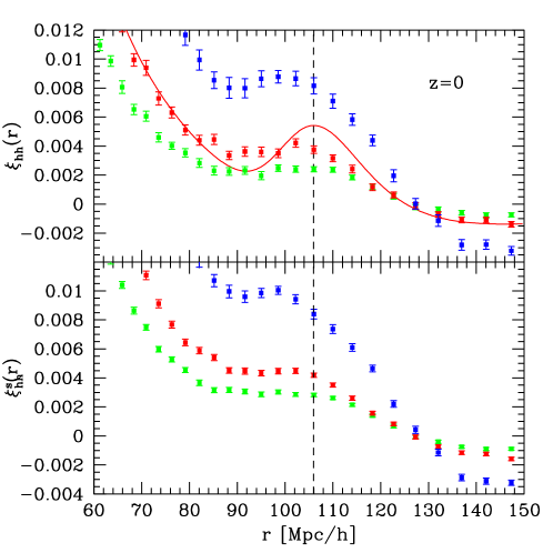
Figure 1 shows the auto-correlation functions of the halos in each of the selected mass bins in our $z=0$ outputs. Top and bottom panels show $\xi(r)$ and $\xi^{\rm s}(r)$, the real and redshift space correlation functions. We have chosen to show $\xi(r)$ rather than $r^{2}\xi(r)$ because, as discussed earlier, the peak in the former is more directly related to the sound horizon scale $r_{s}$. The error bars on the data points come from the scatter around the mean value of $\xi$ as measured in the fifty realizations (i.e. from the diagonal elements of the covariance matrix divided by the square-root of the number of realizations, which for our case is: $\sqrt{50}\sim 7$).

The solid line in the top panel shows the dark matter correlation function predicted by linear theory, multiplied by a constant factor so that the curve approximately matches the signal seen in the intermediate mass bin on scales $r\leq 80\,h^{-1}\,{\rm Mpc}$. The vertical dashed line shows the location of the local maximum in this function: $106\,h^{-1}\,{\rm Mpc}$. Considering the results in real space (top panel), the figure clearly shows that the local maxima of the measured correlation functions are systematically shifted to smaller scales compared to this mark. Moreover, it appears that the magnitude of the shift steadily increases with halo mass. Turning to the results in redshift space, we see that this effect is even more pronounced.

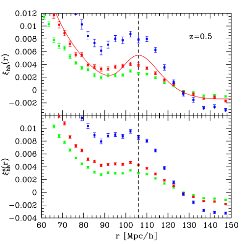
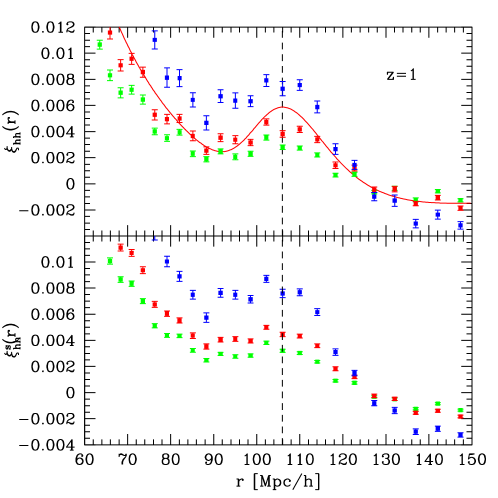
Figures 2 and 3 show results at redshifts, $z=0.5$ and 1. Although the distortions from the linear case appear to be slightly smaller, we again see clearly that the trends are similar to those of the redshift zero case.

We now draw attention to another point of interest. As is expected, these selected halo samples are significantly more clustered than the mass. The large-scale bias factors, as measured by the (square root of the) ratio of the halo correlation function to that of the measured dark matter on scales $\sim 70\,h^{-1}\,{\rm Mpc}$ (where nonlinear effects appear to be small) are $b=1.4,~{}1.8,~{}2.6$ for the $z=0$ halos, $b=1.9,~{}2.3,~{}3.2$ for the $z=0.5$ halos, and $b=2.5,~{}3.0,~{}3.9$ for the $z=1$ halos – with the most massive halos having the largest bias parameters. What is not so obvious now is that the halo clustering signal for each bin at the three different redshifts is almost constant in time. For reference, consider the linear theory growth factor which is smaller by a factor of 0.785 between redshifts $z=0$ and $0.5$, so the amplitude of $\xi_{\rm dm}$ drops between at $z=0$ and $0.5$ by a factor of $\sim$0.615. This result is a direct consequence of studying the signal at fixed comoving number density: whilst the clustering of the mass is much smaller at higher redshift, the high redshift halos are significantly more biased. At fixed number density, the two effects approximately cancel out, keeping the net clustering signal fixed. This is important in view of the fact that galaxies of approximately constant comoving density represent a popular choice for the target sample galaxy to measure the BAO signature over a range of redshifts, i.e. the Luminous Red Galaxies (LRG).

III.3 Statistical properties and model fitting

In this section we examine the statistical properties of the halo-halo correlation functions and present our model fitting analysis.

Figure 4 shows again the simulation results in real space and for the smallest (top) and largest (bottom) bins in halo mass, at $z=0$ (left) and $z=1$ (right). Figure 5 shows again the results in redshift space. In each panel, symbols show the mean value of $\xi^{\rm hh}$ for the given bin in $r$, averaged over the 50 simulations; shaded regions show the standard deviation over the 50 realizations, and error bars show the error on the mean (they are smaller than the shaded regions by a factor of $\sqrt{50}\approx 7$).

The first point to note is that the scatter amongst realizations is remarkable, given that each one of our boxes is about three times larger than the volume probed by the SDSS LRG sample. We further emphasize that at least in redshift space this is likely to be a lower bound on the true underlying scatter, since there is no contribution to the variance from virial motions of the dark matter particles or galaxies. Clearly, enormous volumes will be required to measure $\xi^{\rm hh}$, and thus the galaxy correlation function, to the precision required for percent precision cosmology, and this justifies our earlier assertion at the beginning of this Section.

Comparing now the scatter exhibited in the $z=0$ real space low mass halo sample with that found for the high mass sample, at a first glance we see that the scatter appears to decrease as halo mass increases; and this trend is also exhibited in redshift space data. However as one goes to higher redshifts no obvious trend is apparent between low and high mass samples. Comparing halo samples at the same fixed number density but at different epochs, we see that the scatter is much reduced for the low mass halo sample, but roughly constant for the higher mass sample. This suggests that what is meant by ‘high’ or ‘low’ mass is a very subjective quantity: ‘low’ mass here must mean relative to the typical halo mass at that epoch. However as we shall show shortly these trends with halo mass and measured epoch can not be characterized so naïvely.

We now turn to our modeling of the data. Based on our discussion from Section II, we now attempt to fit the correlation functions by assuming that each can be described as a linearly biased version of the linear theory correlation function, smoothed with a Gaussian filter. There are thus two free parameters for such fits–the scale of the Gaussian smoothing filter $R_{\rm G}$ and the overall amplitude of the bias, which we define $b_{1}^{2}\equiv{\xi}^{\rm hh}(r)/\xi_{\rm Lin}(r)$, where ${\xi}^{\rm hh}(r)$ is the halo-halo correlation function. Note that for this theoretical case we shall assume that the transfer function and hence the cosmological model are fully specified, which for our simulations they are of course, however in reality one should consider fitting for these parameters jointly with other cosmological parameters, albeit with constraints from external data i.e. CMB etc., since these should not be considered known a priori for a realistic case.

The best-fit model parameters for each sample were determined by generating a 2D cubical grid of models over the ranges $b_{1}\in\left[0.5,10.0\right]$ and $R_{f}\in\left[0.5,10.0\right]$, spaced by steps of 0.01, and then computing the $\chi^{2}$ for each, with the final best-fit model being identified as the one with the minimum returned value. Explicitly the $\chi^{2}$ we minimize is

$$\chi^{2}(\hat{b}_{1},\hat{R}_{f})={\overline{\bf Y}}^{T}\hat{C}_{\left<\xi^{\rm hh}\right>}^{-1}{\overline{{\bf Y}}}\ ,$$ (10)

where we define the ensemble average difference vector

$${\overline{\bf Y}}\equiv{{\overline{{\hbox{\BF y}}}}-{\hbox{\BF y}}_{\rm mod}({\bf x}|\hat{b}_{1},\hat{R}_{f})}\ ,$$ (11)

with ${\bar{{\hbox{\BF y}}}}=\left({\bar{\xi}}^{\rm hh}_{1},\dots,{\bar{\xi}}^{\rm hh}_{N}\right)$ and ${\bf x}=\left(r_{1},\dots,r_{N}\right)$, and where ${\hbox{\BF y}}_{\rm mod}$ is a vector of model values. $\hat{C}_{\left<\xi^{\rm hh}\right>}$ is our estimate of the covariance matrix of the mean correlation functions

$$\hat{C}_{\left<\xi^{\rm hh}\right>}\equiv\left[{\overline{{\hbox{\BF y}}^{T}\otimes{\hbox{\BF y}}}}-{\overline{{\hbox{\BF y}}}}^{T}\otimes{\overline{{\hbox{\BF y}}}}\right]/N_{\rm real}\ ,$$ (12)

where $\otimes$ is the direct product operator and we divide by the number of realizations, $1/N_{\rm real}$, because we are estimating the covariances of mean quantities. The inversion of the above Covariance matrix was performed using the SVD algorithm Press et al. (1992). The models were fit over the range of scales $(65\,h^{-1}\,{\rm Mpc}<r<140\,h^{-1}\,{\rm Mpc})$ in 21 equal bins in radius giving $\sim 3.5\,h^{-1}\,{\rm Mpc}$ per bin.

     

     

Figure 4: Mean (solid points), scatter (shaded region) and error on the mean (error bars) for the halo-halo correlation functions measured in the ensemble of 50 simulations. The long dashed curves show the linearly biased, linear theory; the central solid curve shows linear theory, smoothed with a Gaussian filter radius $R$ and linearly biased $b$ (best fit values for these parameters are expressed in the figure annotations). The inner and outer solid curves enclosing the best fit model show the expected scatter in the continuum limit and the discrete Poisson sample limit, respectively – see text for full explanation. The vertical lines represent the local maximum of the linear theory $\xi$ (right most dash line) and the best fit smoothed linear theory model (solid line) and the best-fit Tchebychev polynomial fit (triple dot dashed lines). The bottom panels show the ratio of the measurements to the central solid line and again the error bars are the errors on the mean.

     

     

Figure 5: Same as previous figure, but in redshift space.

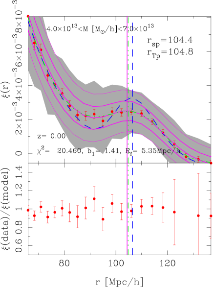
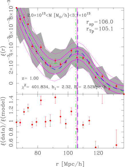
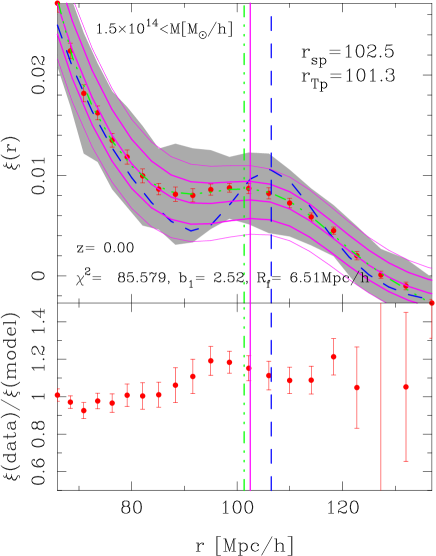
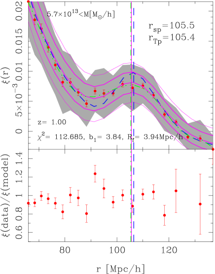
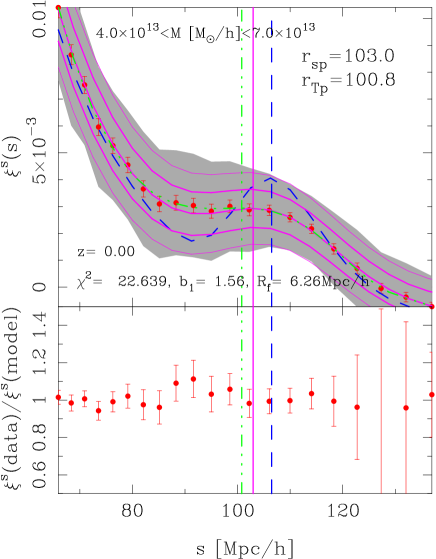
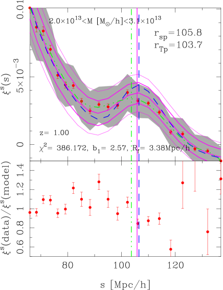
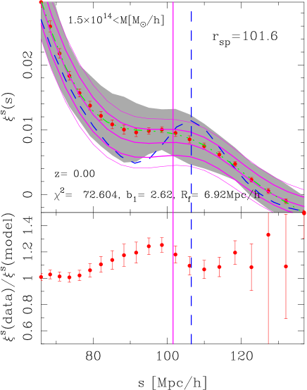
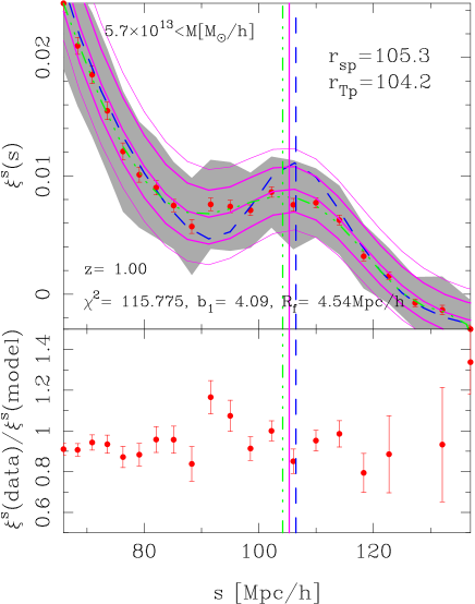
Consider now the three thin solid curves, the central line represents the best-fit smoothed and scaled linear theory correlation function; and the best-fit values for $b_{1}$ and $R_{f}$, along with their respective $\chi^{2}$ values are also reported in each panel. Interestingly, we note that the bias factors in the redshift space figures, recovered from this fitting procedure, roughly agree with our earlier estimates from simply considering the data points around $r\sim 70{\rm Mpc}/h$. For comparison the dashed lines show the best-fit unsmoothed linear theory correlation function with a linear bias. Clearly this model does not provide a reasonable fit to the simulation data over the range of scales presented.

We may now make a prediction for the variance of the correlation function in each bin by assuming that the underlying density field from which the correlation functions were generated is well described by a Gaussian random field. Following Bernstein (1994); Feldman, Kaiser & Peacock (1994); Scoccimarro, Zaldarriaga & Hui (1999); Meiksin & White (1999); Cohn (2006), the covariance matrix for bin averaged correlation function, in the limit of small bin sizes $\Delta r/r\ll 1$, can be written

$$\left[C_{\bar{\xi}^{\rm hh}}\right]_{ij} \equiv \langle{\bar{\xi}}^{\rm hh}_{i}\bar{\xi}^{\rm hh}_{j}\rangle-\langle\bar{\xi}^{\rm hh}_{i}\rangle\langle\bar{\xi}^{\rm hh}_{j}\rangle$$ (13)

$$= \frac{1}{V_{\mu}}\int{dk\,k^{2}\over 2\pi^{2}}\,j_{0}(kr_{i})j_{0}(kr_{j})\sigma^{2}_{P^{\rm hh}}(k)\ ,$$

where $\bar{\xi}^{\rm hh}_{i}$ is the bin averaged correlation function in bin $i$, $V_{\mu}$ is the simulation volume, $j_{0}=\sin(x)/x$ is the zeroth order spherical Bessel function and where $\sigma^{2}_{P^{\rm hh}}$ is the Gaussian variance per mode in the halo–halo power spectrum, which for a discrete Poisson sampling of the halo field, can be written

$$\sigma^{2}_{P^{\rm hh}}(k)=2\left[P^{\rm hh}(k)+\frac{1}{\bar{n}_{H}}\right]^{2}\ ;$$ (14)

where we write our smoothed halo-halo power spectrum, at linear order in the over-density perturbation and bias, as

$$P^{\rm hh}(k|R_{f})\equiv V_{\mu}\langle\left|\delta^{\rm h}(k|R_{f})\right|^{2}\rangle=\hat{b}_{1}^{2}P_{\rm Lin}(k)W^{2}(k\hat{R}_{f})\ .$$ (15)

For the purposes of numerical evaluation of the above formulae, we follow Cohn (2006) and note that one may rewrite the contribution to the covariance coming from the term $1/\bar{n}_{H}^{2}$ as follows:

$$\frac{2}{V_{\mu}\bar{n}_{H}^{2}}\int\frac{d^{3}\,k}{(2\pi)^{3}}\,j_{0}(kr_{i})\,j_{0}(kr_{j})=\delta^{K}_{i,j}\frac{2}{\bar{n}_{H}^{2}V_{\mu}V(r_{i})}\ ,$$ (16)

where the volume associated with each shell is: $V(r_{i})=4\pi r_{i}^{2}\Delta r$. The variance in the correlation function is then simply given by setting $i=j$ in Eq. (13). Using our Gaussian smoothed linear model for $P^{\rm hh}(k)$ ensures that the integrals over the Bessel functions converge rapidly. For a more detailed discussion of convergence properties see Cohn (2006).

Considering again the best-fit smoothed model in each panel, surrounding it are two sets of solid lines, a thick inner set and a thin outer set. The inner lines show the scatter between realizations that one would predict using the continuum limit of Eq. (14), that is when $1/\bar{n}_{H}\rightarrow 0$. In this case, the theoretical predictions clearly underestimate the true scatter in $\xi^{\rm hh}$ for all bins in halo mass, with the discrepancy being slightly worse for the lowest mass bin. The outer solid curves now show the effect of including the discreteness contribution from $1/\bar{n}_{H}$ in Eq. (14). Note that in implementing Eq. (16) it was essential to correctly account for the binning in the correlation function. In most cases, and especially for the $z=1$ correlations, this additional contribution provides a much improved description of the measured scatter. However, at low redshift and for the lowest mass haloes considered the theoretical estimate of the scatter appears too small. This is likely a consequence of the growing non-Gaussian contributions to the variance from the connected trispectrum and bispectrum, Scoccimarro, Zaldarriaga & Hui (1999); Meiksin & White (1999); Neyrink & Szapudi (2007) and that the discrepancy between high and low-mass halo samples may be caused by the effect of non-linear halo bias terms entering the variance estimate.

Returning to the issue of how the scatter depends on the samples. Considering again our expression for the Gaussian error on the power spectrum, Eq. (14), we see that the relative error per mode can be written:

$$\frac{\sigma_{P}^{\rm hh}}{P^{\rm hh}}=\sqrt{2}\left[1+\frac{1}{\bar{n}_{H}b_{1}^{2}P_{\rm Lin}(k,z)}\right]\ .$$ (17)

Thus we see that the relative scatter may increase in three ways: as halo bias decreases; as halo number density decreases; and as the power spectrum amplitude changes with time. For our constructed samples these effects conspire in such a way that it is no longer trivial to isolate trends. Rather than attempting to follow this path we simply note that to say anything substantiative we must consider the full covariance matrix, since a decrease in diagonal covariance can be traded for an increase in off-diagonal covariance – which is just as important in the fitting. We shall reserve the important issue of power spectrum and correlation function covariance for a future study.

Lastly, we note that for very sparse samples of haloes the theoretical prediction given by Eq. (13) actually represents a lower bound, since there should be a further (non-Gaussian) shot-noise contribution of the order $\delta^{K}_{i,j}2\bar{\xi}^{\rm hh}_{i}/\left[\bar{n}_{H}^{2}V_{\mu}V(r_{i})\right]$ Cohn (2006). However, for our purposes this term is unimportant, since $\bar{\xi}^{\rm hh}_{i}\ll 1$.

Table 2: Shifts in the BAO peak position as a function of halo sample in real space.

SAMPLE	$R_{f}\ [\,h^{-1}\,{\rm Mpc}]$	$b_{1}$	$\delta_{\rm Sp}\ [\%]$	$\delta_{\rm Tp}\ [\%]$	$\delta_{\rm Phys}\ [\%]$
	$z=0$     $z=1$	$z=0$     $z=1$	$z=0$     $z=1$	$z=0$     $z=1$	$z=0$     $z=1$
$M_{1}$	5.35     2.52	1.41     2.32	1.5     0.00	1.10     0.85	0.38     0.85
$M_{2}$	5.25     2.52	1.71     2.72	1.32     0.00	5.20     0.09	2.92     0.09
$M_{3}$	6.51     3.94	2.52     3.94	3.30     0.47	4.40     0.57	1.13     0.09

Table 3: Shifts in the BAO peak position as a function of halo sample in redshift space.

SAMPLE	$R_{f}\ [\,h^{-1}\,{\rm Mpc}]$	$b_{1}$	$\delta_{\rm Sp}\ [\%]$	$\delta_{\rm Tp}\ [\%]$	$\delta_{\rm Phys}\ [\%]$
	$z=0$     $z=1$	$z=0$     $z=1$	$z=0$     $z=1$	$z=0$     $z=1$	$z=0$     $z=1$
$M_{1}$	6.26     3.38	1.56     2.57	2.83     0.18	4.90    2.16	2.07     1.98
$M_{2}$	6.97     4.04	1.91     2.88	4.60     0.66	6.13    1.20	1.51     0.57
$M_{3}$	6.92     4.54	2.62     4.09	4.40     0.70	NA     1.80	NA     1.10

III.4 Evidence for shifts

We now illustrate very clearly the effects of ‘apparent’ shifts on the peak position of the correlation function, arising from the operation of smoothing, and explore the hypothesis that the peak position also exhibits large-scale ‘physical’ motion.

Before we commence with this investigation we note that since our simulations used the transfer function generated at $z=49$, our linear theory acoustic peak is slightly less sharp than that which obtains from using the transfer function at $z=0$ (which is more correct). This means that the apparent shifts will be overestimated, since, as was discussed in Section II, smoothing affects more a weaker peak. For dark matter clustering, a calculation using renormalized perturbation theory Crocce & Scoccimarro (2007) shows that the apparent shift is overestimated by about a factor of two by using the transfer function calculated at $z=49$. However, the physical shifts are not changed significantly.

Considering again Figs 4 and 5, as noted above, the (blue) dashed lines in each panel show the associated biased but unsmoothed linear theory correlation functions, and clearly these do not provide a good fit to the data. The corresponding vertical dash lines show the position of the local maximum of this curve – the unperturbed acoustic peak: $r_{\rm Up}=106\,h^{-1}\,h^{-1}\,{\rm Mpc}$. Now consider the best fit smoothed models (central solid magenta), these clearly (by eye) provide a much improved fit to the data. On finding the local maximum of these smoothed models, we see that in all cases the peak has been shifted to smaller scales. These are denoted in each panel by the solid magenta vertical lines and with their values reported in the top right of each panel as $r_{\rm Sp}$, with ‘Sp’ meaning smoothed peak.

Considering these smoothed model inferred peak positions, we note several important trends:

• All maxima lie on smaller scales than $r_{\rm Up}$;

• For halo samples considered at the same epoch and in both real and redshift space, the shifts from $r_{\rm Up}$ increase with increasing halo mass;

• Considering halo samples of the same fixed number density at different redshifts, the shifts are reduced for the higher redshift samples;

• Shifts are increased in the redshift space;

• Best fit filter scale increases with halo mass.

The spread of values in the smoothed model shifts $\delta_{\rm Sp}\equiv{\left[r_{\rm Up}-r_{\rm Sp}\right]}/r_{\rm Up}$, span the range $\delta_{\rm Sp}\sim 1.0\%-5\%$, with the largest values being obtained as per the trends described above. These shifts, it can be argued Eisenstein, Seo & White (2006), fall under the banner of apparent shifts – arising from the local collapse and rearrangement of matter. However, following our discussion of the transfer function, we expect that these shifts would be reduced by a factor of $\sim 2$ for the $z=0$ transfer function: $\delta_{\rm Sp}\sim 0.5\%-2.5\%$. We also note that in the recent literature a number of procedures have been proposed to tackle these apparent shifts and, modulo the choice of filter function, most of these methods should be able to successfully correct for these effects. However, we now draw attention to the last of our bullet points and note the fact that the best fit filter scale $R_{f}$, increased with halo mass. This implies that methods that are tested and tuned to extract BAO information using only the dark matter distribution will fail to incorporate this effect – we return to this in Sec. III.5.

Turning now to the question of ‘physical’ shifts, it is clear that the smoothed model does not provide consistently good fits to the measurements for all our samples. To see this more clearly, the bottom section of each panel shows the ratio of the measured points to the best-fit smoothed linear model. From examination of these results it is clear that there is some evidence for structure in these residuals — typically, on scales smaller than the true acoustic peak position we find that the data points lie above the best fit smoothed model. This trend is most apparent for the present day high mass halo samples, but is less clear for the lowest mass. This can be further quantified by use of the $\chi^{2}$ test as an indicator for the ‘goodness-of-fit’: for $N=21$ data bins and $m=2$ parameters, the probability $P(\chi^{2}>36.19|n=19)=0.01$. Thus on inspection of the $\chi^{2}$ values in Figs 4 and 5 we see that only in two instances are the mean data in agreement with this and these are for the present day low mass samples in real and redshift space. Based on these data we are led to reject our null hypothesis and accept the possibility that there is a physical motion of the peak.

One alternative to the ‘physical motion’ hypothesis is that the filter choice is somehow special – and had we chosen the ‘special’ filter then this would reconcile our results. This view is problematic, since in order to model all of the above trends such a filter would have to be highly contrived. Thus, based on the above evidence, it seems that something like the second term in Eq. (1) is present and generating a shift in the position of the peak.

In the next section, we provide details of a physically motivated model that may offer some insights into the origin of the dependence on halo mass of the shifts in the acoustic peak position.

Before continuing, it is of interest to characterize the peaks in the correlation function data using a purely artificial parameterized model that simply matches the data in the least square sense. For this we write the model of the correlation function as a sum over the orthogonal Tchebyshev polynomials, $T_{i}(x)$, i.e.

$$y_{\rm mod}(r)=\xi^{\rm hh}(r)=\sum_{i=0}^{m}a_{i}T_{i}[x(r)]\ ;$$ (18)

and $x(r)$ here is a mapping that transforms the $r$-range into the range $x\in\left[-1,1\right]$ so that we may use the normalized polynomials. We then, as before, find the coefficients $a_{i}$ that minimize our $\chi^{2}$ Eq. (10) and polynomials up to degree 9 were used to describe the data and, for simplicity, in the fitting we have used only the diagonal elements of the covariance matrix to make the constraints. These artificial models along with the locations of their local maxima at the acoustic scale are presented in Figs 4 and 5 as the (green) triple-dot dash curves, and the values of the maxima are noted in the top-right hand corner of each panel as $r_{\rm Tp}$. For the high mass samples the shifts, $\delta_{\rm Tp}\equiv[r_{\rm Up}-r_{\rm Tp}]/r_{\rm Up}$, are significantly enhanced relative to linear model, and for the case of the highest mass halo sample at $z=0$ in redshift space, the best fit model had no local maximum.

We may now be more definite in what we mean by a physical shift: we shall say the percentage physical shift away from the true peak is $\delta_{\rm Phys}\equiv\left|\delta_{\rm Sp}-\delta_{\rm Tp}\right|$. The physical shifts appear to be smaller than the apparent shifts and are roughly of the order $\sim 0.4-3.0\%$ at $z=0.0$ for real and redshift space data and they are somewhat mitigated at higher redshifts. Tables 2 and 3 collect together the apparent, total and physical shift values for the halo samples in real and redshift space, respectively. As we shall discuss in the following section these physical shifts are not accounted for in the recent methods proposed to correct for the non-linear evolution of the BAO peak position.

Figure 6: Expected behavior of the residuals in the correlation function arising from the alternative approach to BAO model fitting of Eisenstein, Seo & White (2006), where the broad-band, but smooth, linear power is restored. From top to bottom the lines show the effects where a smoothing scale of $R_{f}=\{2,4,8\}\,h^{-1}\,{\rm Mpc}/h$ were taken. This method does not replicate the $S$ shaped structure of the residuals found in the data.

III.5 Alternative BAO reconstruction methods

Recently a number of procedures have been proposed to correct the BAO peak position for the effects of the large scale structure systematics (see for example Seo & Eisenstein (2005); Eisenstein, Seo & White (2006); Huff et al. (2006); Percival et al. (2007a); Angulo et al. (2007)). These methods essentially allow for smoothing in configuration space and possible broad band tilts in the underlying power spectrum. Since the correlation function is the Fourier space dual of the power spectrum, these methods should also be equally applicable in configuration space.

Firstly, consider those methods that attempt to correct the measured power spectrum for tilting by fitting away an arbitrary constant – this is in response to ideas from the Halo Model that lead us to consider a generalized Poisson shot-noise correction (see for example Schulz & White (2006)). On Fourier transforming this model it does nothing to the peak of the correlation function and so may be dismissed.

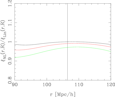
Secondly, consider a model that is designed to damp out the acoustic oscillations, but then restore the linear theory power using a smooth (no BAO) version of the linear power Eisenstein, Seo & White (2006), e.g.

$$P_{\rm NL}(k|R)={\rm e}^{-k^{2}R^{2}}\,b^{2}P_{\rm Lin}(k)+(1-{\rm e}^{-k^{2}R^{2}})\,b^{2}P_{\rm Lin}^{\rm smooth}(k),$$ (19)

In the configuration space the first term transforms into the smoothed linear model Eq. (15), and as we saw this will generate apparent shifts. Considering the second term, we see that this function has no information about the acoustic scale. Fig. 6 shows that this model for a range of smoothing filter scales - in all cases, it is flat around the acoustic peak. Moreover, the ratio $\xi_{\rm NL}(r|R)/\xi_{\rm Lin}(r|R)<1$ for all smoothing scales, whereas the measured residuals can exceed unity on scales smaller than the acoustic peak (cf. Figures 4 and 5). We therefore deduce that a model like equation (19) is inadequate.

Lastly, we note that a more sophisticated method for correcting the spectrum for the non-linear systematics was proposed by Percival et al. (2007a). However, this method was recently looked at in great detail by Crocce & Scoccimarro (2007), for the most optimistic case - dark matter in real space. There it was shown that, although the method accounts for broadband tilting of the underlying power spectrum, it was unable to correct for the shift of the peak due to mode-coupling. Since these mode coupling terms are even more enhanced in the halo-halo power spectrum (see Smith, Scoccimarro & Sheth (2007)) we expect that this method will not correct for all of the physical shifts found in the previous section.

In passing, we note that it is not straightforward to draw a direct connection between what we call the physical shift and what Crocce & Scoccimarro (2007) describe as mode-coupling shifts. It is likely that what we have called a physical shift is an underestimate of the mode-coupling effects. To understand why, we note that whilst the Renormalized Perturbation Theory formalism has yet to be extended to Haloes, we may suppose that the RPT decomposition of the 2-pt clustering signal will still be valid, i.e. there is some propagator which multiplies the linear theory power, and some sum of mode-coupling terms. Suppose the halo propagator has almost the same form as the dark matter propagator, so the effects of the non-linear bias mainly affect the mode coupling pieces. Since the propagator is akin to a Gaussian smoothing term, this term acts just like the simple Gaussian smoothing model we fit to the simulation data. If the effects of the other (mode-coupling) term were negligible, or did not depend strongly on halo mass, then we would expect the scale of the best fit smoothing filter to also be independent of halo mass. It is not, suggeting that the mode-coupling term depends on halo mass. That the scale of the best-fit smoothing filter is larger for the more massive halos (Table 2 and 3) indicates that our best-fitting Gaussian filter is trying to account for some of the shifting that is actually due to the mode-coupling terms.

We shall now pursue an analytic approach that we think provides insight in to the physics behind the shifts.

IV A physical model for the shifts

This section presents a simple physical model for estimating the effects of nonlinear clustering and bias on the position of the local maximum of the correlation function. Crocce & Scoccimarro (2007) discuss a more accurate model for the correlation function of the dark matter; the approach below allows one to address how the peak shifts are affected if the measured correlation function comes from a biased tracer of the dark matter field.

IV.1 The pair conservation equation

The perturbed continuity equation for the collisionless CDM fluid can be written,

$$\frac{\partial\left[1+\delta({\bf x},\tau)\right]}{\partial\tau}+\nabla\cdot\Big{[}(1+\delta({\bf x},\tau))\,{\hbox{\BF v}}({\bf x},\tau)\Big{]}=0.$$ (20)

where $\delta({\bf x},\tau)\equiv[\rho({\bf x},\tau)-\rho_{\rm b}(\tau)]/\rho_{\rm b}(\tau)\ ,$ is the dimensionless density perturbation at comoving position ${\bf x}$ and conformal time $\tau$ ($d\tau\equiv dt/a(t)$, where $a(\tau)$ is the expansion factor from the Friedmann equation); $\rho_{\rm b}(\tau)$ is the homogeneous background density; and ${{\hbox{\BF v}}}({\bf x},\tau)\equiv{\bf x}^{\prime}\equiv d{\bf x}/d\tau$ is the proper peculiar velocity field Bernardeau et al. (2002); Peebles (1980).

We can now use Eq. (20) at position 1, say, multiply by $(1+\delta_{2})$ for position 2, and add the same expression with indices $1$ and $2$ interchanged $[\delta_{i}\equiv\delta({\bf x}_{i})]$. Taking expectation values of the result yields the pair conservation equation Peebles (1980); Nityananda & Padmanhbhan (1994); Fisher (1995); Juszkiewicz et al. (1999):

$$\frac{\partial[1+\xi({\bf r},\tau)]}{\partial\tau}+\nabla\cdot\Big{[}[1+\xi({\bf r},\tau)]\,{\hbox{\BF v}}_{12}({\bf r},\tau)\Big{]}=0,$$ (21)

where the divergence is with respect to the vector that separates the pair ${\hbox{\BF r}}={\hbox{\BF x}}_{1}-{\hbox{\BF x}}_{2}$, and the pairwise infall velocity is

$${\hbox{\BF v}}_{12}({\bf r},\tau)\equiv\frac{\langle(1+\delta_{1})(1+\delta_{2})({\hbox{\BF v}}_{1}-{\hbox{\BF v}}_{2})\rangle}{[1+\xi({\bf r},\tau)]};$$ (22)

where by statistical isotropy we used that $\left<\delta_{1}{\hbox{\BF v}}_{1}\right>=\left<\delta_{2}{\hbox{\BF v}}_{2}\right>=0$.

We can rewrite Eq. (21) in a more convenient form, by changing time variable from conformal time $\tau$ to the linear growth factor $D_{+}$. In particular, if

$$\eta\equiv\ln D_{+},$$ (23)

then $d\tau=d\eta/({\cal H}f)$, where ${\cal H}=d\ln a/d\tau$ and $f=d\ln D_{+}/d\ln a$. We may also write velocities in a similar fashion and scale out their dependence on linear theory. Namely, ${\hbox{\BF v}}=-{\cal H}f{\hbox{\BF u}}$, where $\nabla\cdot{\hbox{\BF u}}=\delta$ in the linear theory. Then, dividing Eq. (21) by $[1+\xi({\bf r},\tau)]$ yields,

$$\frac{\partial\ln[1+\xi(r,\eta)]}{\partial\eta}-{\hbox{\BF u}}_{12}\cdot\nabla\ln[1+\xi(r,\eta)]=\nabla\cdot{\hbox{\BF u}}_{12}({\bf r},\eta)\ .$$ (24)

Owing to the fact that large-scale flows have no vorticity, the pairwise velocities are directed along the separation unit vector $\hat{{\bf r}}$, so ${\hbox{\BF u}}_{12}=u_{12}\,\hat{{\bf r}}$. Hence Eq. (24) becomes,

$$\frac{\partial\ln[1+\xi(r,\eta)]}{\partial\eta}-u_{12}(r,\eta)\frac{\partial\ln[1+\xi(r,\eta)])}{\partial r}=\Theta(r,\eta)\ ,$$ (25)

where we have defined $\Theta(r,\eta)\equiv\nabla\cdot[u_{12}(r,\eta){\hat{\bf r}}]$ to be the divergence of the pairwise infall velocities $u_{12}(r)$. Note, that this equation may be thought of as a differential equation for $\ln(1+\xi)$ given an ansatz for $u_{12}$ Nityananda & Padmanhbhan (1994), or ‘vice-versa’ Juszkiewicz et al. (1999).

IV.2 Solution by characteristics

The general solution of Eq. (25) can be found by the method of characteristics (see for example Landau & Lifschitz (1959)), which illustrates quite clearly how any feature in the correlation function will move as clustering develops.

The continuity equation (and thus the pair conservation equation) is a prime example of a hyperbolic partial differential equation. Information propagates from the initial conditions to the final conditions through curves, called characteristics. The characteristics are simply the equations of motion of pairs,

$$\frac{dr}{d\eta}=-u_{12}(r,\eta).$$ (26)

The solution of this equation gives $r(\eta)$, and this converts the left hand side of Eq. (25) into a total derivative. Thus, one obtains an ordinary differential equation along the characteristics:

$$\frac{d\ln[1+\xi(r,\eta)]}{d\eta}=\Theta(r,\eta)\ ,$$ (27)

and it should be understood that it is a function of time $\eta$ only, after using the characteristic solution $r(\eta)$, Eq. (26). Thus Eq. (27) simply gives the logarithmic rate of change of the two-point correlation function as it evolves along the characteristic curve. The fully evolved correlation function may then be obtained straightforwardly, at any chosen epoch, through integration along the characteristic between the initial and final epoch:

$$1+\xi(r,\eta) = \Big{(}1+\xi_{0}[r_{0}(r,\eta)]\Big{)}$$ (28)

$$\times\exp\Big{[}\int_{0}^{\eta}\Theta[r_{\eta^{\prime}}(r,\eta),\eta^{\prime}]\,d\eta^{\prime}\Big{]},$$

where $r_{0}(r,\eta)$ is the initial separation that corresponds to $r$ at time $\eta$, and similarly for $r_{\eta^{\prime}}$. The exponential factor comes from the fact that the correlation function is not conserved along characteristics because the right hand side of Eq. (27) is non-zero. Since we are mostly interested in significant growth after the initial perturbations are laid down ($\eta\gg\eta_{0}$), the term in the first parenthesis can be safely approximated as unity. Hence, all the evolution is encoded in $\Theta$ and the characteristics. Note that this solution is exact; it only becomes useful, though, if one can model the pairwise infall velocities.

Figure 7: The flow of characteristics in linear theory for initial separations close to the acoustic peak of the two point function, every 1 $\,h^{-1}\,{\rm Mpc}$. For each scale we show results for dark matter (solid, solutions of Eq. 32), and linearly biased tracers (solutions of Eq. 50) having $z=0$ bias factors of $b=1.4$ (dashed) and $b=2$ (dot-dashed). The peak in the linear correlation function is located at $r=106\,h^{-1}\,{\rm Mpc}$ for the cosmological model we use in this paper.

IV.3 Linear theory velocities

For what follows, it will be convenient to define

$$\bar{\xi}_{0}(r_{0},\eta_{0})\equiv e^{2\eta_{0}}\,\frac{3}{r}\int\frac{P_{0}(k)}{k}\,j_{1}(kr)\,d^{3}k,$$ (29)

where $P_{0}(k)$ is the power spectrum at some initial time $\eta_{0}\equiv 0$ and where $j_{1}(y)\equiv[\sin(y)-y\cos(y)]/y^{2}$ is the first order spherical Bessel function. In linear theory, pairwise infall velocities, at time $\eta$, can be written Peebles (1980); Fisher (1995)

$$u_{12}(r,\eta)=2\,{\rm e}^{2\eta}\,\int\frac{P_{0}(k)}{k}\,j_{1}(kr)\,d^{3}k=\frac{2r}{3}\,{\rm e}^{2\eta}\,\bar{\xi}_{0}(r)\ .$$ (30)

velocityfield . The divergence of pairwise velocities in linear theory can be obtained directly from Eq. (30) by taking the divergence,

$$\Theta(r,\eta) = \nabla_{r}\cdot[u_{12}(r)\hat{{\bf r}}]\equiv\frac{1}{r^{2}}\frac{\partial}{\partial r}[r^{2}u_{12}(r)]\ ,$$ (31)

$$= 2\,{\rm e}^{2\eta}\,\int P_{0}(k)\,j_{0}(kr)\,d^{3}k\ ,$$

$$= 2\,{\rm e}^{2\eta}\,\xi_{0}(r)\ ,$$

with $\xi_{0}$ the initial (linear) correlation function at $\eta_{0}=0$.

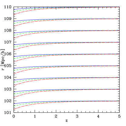
Eq. (30) allows us to solve for the characteristics in linear theory. Two-point information at separation $r_{0}$ and time $\eta_{0}=0$ propagates by time $\eta$ to a separation $r$ (less than $r_{0}$, due to clustering) so that, from Eq. (26)

$${\rm e}^{2\eta}-1=\int_{r}^{r_{0}}\,\frac{3}{\bar{\xi}_{0}(r)}\frac{dr}{r}\ .$$ (32)

Figure 7 shows the solution of this equation ($r$ as a function of redshift) for initial separations $r_{0}$ close to the acoustic peak of the two-point correlation function. If this were the only effect, i.e. if the right hand side of Eq. (27) were zero, then the correlation function would be conserved along the characteristics (solid blue line shown in Fig. 7) and this alone would give about $0.2\%$ shift in the acoustic peak position by $z=0$. However, as mentioned above, the correlation function grows along the characteristics. This growth is governed by the divergence of the infall velocities, and, for large $\eta$, it is this contribution which dominates. Indeed, we have not yet even included the linear amplification of the correlation function, resulting from the right hand side in Eq. (27).

Including the divergence of infall velocities using Eq. (31), makes Eq. (28) for the two-point function

$$1+\xi(r,\eta) = \Big{(}1+\xi_{0}[r_{0}(r,\eta)]\Big{)}$$

$$\times\exp\Big{[}2\int_{0}^{\eta}\xi_{0}[r_{\eta^{\prime}}(r,\eta)]\,{\rm e}^{2\eta^{\prime}}d\eta^{\prime}\Big{]}.$$

If the flow of characteristics caused by the nonlinear term in Eq. (25) is ignored, then $r\approx r_{\eta^{\prime}}\approx r_{0}$, and so

$$1+\xi(r) \approx \Big{(}1+\xi_{0}(r)\Big{)}\,\exp\Big{[}\xi_{0}(r)({\rm e}^{2\eta}-1)\Big{]}$$ (34)

$$\approx 1+\xi_{0}(r)\,{\rm e}^{2\eta}.$$

The final expression follows if the term in the exponential is small; notice that it equals the linear perturbation theory expression for $\xi$ at time $\eta$.

At first sight, the solution of Eq. (LABEL:sol) appears to require many evaluations of Eq. (32). However, the integral over $\eta^{\prime}$ in the exponential piece of Eq. (LABEL:sol) may be transformed using the characteristic curve, whence

$$2e^{2\eta}=d(e^{2\eta}-1)=-\frac{3}{\bar{\xi}(r)}\frac{dr}{r}\ .$$ (35)

Thus on performing this change of variables, the term in the exponential of Eq. (LABEL:sol) becomes

$$\Rightarrow\ 3\int_{r}^{r_{0}}\frac{dr^{\prime}}{r^{\prime}}\,\frac{\xi_{0}(r^{\prime})}{\bar{\xi}_{0}(r^{\prime})}\ .$$ (36)

However, on noting that $d\left[r^{3}\bar{\xi}(r)\right]/r^{3}=3\xi(r)dr/r$, we find that this may be further simplified to

$$\Rightarrow\ \int_{r^{3}\bar{\xi}_{0}(r)}^{r_{0}^{3}\bar{\xi}_{0}(r_{0})}\frac{dx}{x}\ .$$ (37)

Therefore, Eq. (LABEL:sol) is really rather simple:

$$1+\xi(r,\eta)=\Big{(}1+\xi_{0}(r_{0})\Big{)}\,\frac{r_{0}^{3}\,\bar{\xi}_{0}(r_{0})}{r^{3}\,\bar{\xi}_{0}(r)}\ ,$$ (38)

and a single evaluation of Eq. (32) gives $r_{0}(r,\eta)$, and hence the nonlinear value of $\xi(r)$.

IV.4 Connections to previous work

At late times ${\rm e}^{2\eta}\gg 1$. Hence, on the large scales where $\xi_{0}\ll 1$, Eq. (34) implies that $1+\xi(r)\approx\exp[\Xi_{\eta}(r)]$, where $\Xi_{\eta}(r)={\rm e}^{2\eta}\,\xi_{0}(r)$ is the linearly evolved correlation function. This is precisely the relation between the correlation function of a lognormal field and that of the underlying Gaussian field from which it was derived. Of course, this analysis has assumed that $r\approx r_{\eta^{\prime}}\approx r_{0}$; Figure 7 shows that this is inappropriate at late times. Nevertheless, it provides a nice illustration of why the Lognormal has proved to be such a useful approximation, and why the approximation breaks down . Note that, both in linear theory and in the Lognormal approximation for the nonlinear evolution, the position of the acoustic peak does not shift .

Our Eq. (38) has the flavor of an approach pioneered by Hamilton et al. (1991); Nityananda & Padmanhbhan (1994), who argued that

$$1+\bar{\xi}(r,\eta)=(r_{0}/r)^{3}$$ (39)

should provide a good approximation to nonlinear evolution. In effect, their approach sets

$$1+\xi(r,\eta)=\left(\frac{r_{0}}{r}\right)^{3}\,\frac{\partial\ln r_{0}}{\partial\ln r}.$$ (40)

If we set $1+\xi_{0}(r_{0})\to 1$, then we have

$$1+\xi(r,\eta)=\left(\frac{r_{0}}{r}\right)^{3}\frac{\bar{\xi}_{0}(r_{0})}{\bar{\xi}_{0}(r)};$$ (41)

our expression follows from inserting the linear velocities in the characteristics—it is not an ansatz. Note that this relation changes if nonlinear velocities are used.

Figure 8: The divergence of pairwise infall (dark matter) velocities $\Theta$ as a function of scale measured in numerical simulations at $z=0$ (solid squares) and at $z=1$ (solid triangles). In linear perturbation theory, $\Theta/2$ is equal to the linear correlation function – and at $z=0$ and $z=1$ the linear models are represented by solid red and blue lines, respectively. Notice that at $z=1$ the acoustic peak is visible in $\Theta$, but by $z=0$ the nonlinear effects have completely washed out any trace of it.

IV.5 Inaccuracy of linear theory velocities

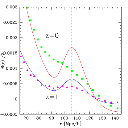
In linear theory the divergence of infall velocities $\Theta(r,\eta)$ is, modulo a factor of two, given by the linear two-point function itself (c.f. Eq 31) and this has a static (independent of $\eta$) peak at the unperturbed position. Hence, there is a competition between $\Theta$, which prefers the peak to stay unshifted, and the flow of characteristics, which induce a shift towards smaller scales (Fig. 7). A consequence of this is that, using linear velocities is expected to underestimate the true peak shift. (The top left panel of Fig. 9 shows this explicitly, as we discuss later.) Using Eq. (38) one obtains a shift of about $0.1\%$ at $z=0$, half of that due to the flow of characteristics.

This underestimate results from the fact that, whilst the pairwise infall velocity may be reasonably well described by linear theory on large scales, its divergence deviates from linear theory more strongly, due to the scale dependence of nonlinear corrections Scoccimarro (2004); Crocce & Scoccimarro (2006b). This is graphically illustrated in Fig. 8. Although $\Theta\propto\xi$ in linear theory, by $z=0$, nonlinear effects have washed out any sign of an acoustic peak in $\Theta$!

In practice, a characteristic that probes scales slightly smaller than the unperturbed acoustic peak will experience more growth of the two-point function at late times. This leads directly to an enhancement that dominates over the effect of the flow of characteristics, and results in a substantially enhanced shift over the linear case (and as we will show this enhancement is about one order of magnitude). In this sense the flow of characteristics only gives a lower bound to the shift in the peak position due to mode coupling. Clearly, in order to proceed, we require a model for the nonlinearity of the infall of pairwise velocities, and in particular its divergence $\Theta$.

IV.6 Beyond linear theory velocities

There are two types of nonlinear contributions to the pairwise infall velocity. This can be seen more clearly by rearranging Eq. (22) into the form,

$${\hbox{\BF u}}_{12}=\frac{\langle(\delta_{1}+\delta_{2})({\hbox{\BF u}}_{1}-{\hbox{\BF u}}_{2})\rangle+\langle\delta_{1}\delta_{2}({\hbox{\BF u}}_{1}-{\hbox{\BF u}}_{2})\rangle}{1+\xi}.$$ (42)

If we insert the standard perturbation theory (hereafter, PT) expansions for $\delta$ and $u$ Bernardeau et al. (2002), then we see that the first term in the numerator is second order in $\delta({\bf x},\eta_{0})$, and the second term is of third order, which in linear theory averages to zero. We can set the denominator equal to unity, since $\xi$ is of order $10^{-3}$ on the scales of interest and we are after much larger ($1-10\%$) effects. As mentioned in the previous subsection, the effects from nonlinear mode-coupling on $u_{12}(r,\eta)$ on these scales are negligible ($\sim 1\%$), and hence play almost no role in shaping the characteristic curves (which, as we said, lead to shifts of only $\sim 0.2\%$ in linear theory for dark matter). They do, however, have a significant impact on the source term in the right-hand-side of Eq. (27), which dictates how fast the two-point function grows along the characteristics.

Eq. (42) thus leads to the following decomposition

$$\Theta(r,\eta)\equiv\Theta_{2}(r,\eta)+\Theta_{3}(r,\eta),$$ (43)

where the two terms on the right-hand-side are defined $\Theta_{2}\equiv 2\nabla\cdot\left<\delta_{1}{\hbox{\BF u}}_{2}\right>$ and $\Theta_{3}\equiv 2\nabla\cdot\left<\delta_{1}\delta_{2}{\hbox{\BF u}}_{1}\right>$. Considering the first term, on using the standard PT expansions for the density and divergence of the velocity field (Bernardeau et al. (2002) and see also footnote velocityfield ), we find that $\Theta_{2}$ can be written

$$\Theta_{2}(r,\eta)=2\,\int P^{\delta\theta}\!(k,\eta)\,j_{0}(kr)\,d^{3}k\ ,$$ (44)

and

$$P^{\delta\theta}\!(k,\eta)={\rm e}^{2\eta}\,P^{\delta\theta}_{0}(k)+{\rm e}^{4\eta}\,P^{\delta\theta}_{\rm 1loop}(k)\ ,$$ (45)

is the cross-power spectrum of the density and velocity divergence expanded to fourth order in the standard PT. The first term is the usual one from linear theory $P^{\delta\theta}_{0}=P_{0}$, and $P^{\delta\theta}_{\rm 1loop}$ is the ‘one-loop’ correction to $P^{\delta\theta}$ from PT. The middle panel of Fig. 6 in Scoccimarro (2004) shows that this term describes rather well (much better than for the density power spectrum) the deviations from linear theory at large scales. Thus,

$$\Theta_{2}(r,\eta)=\Theta_{2}^{0}(r,\eta)+\Theta_{2}^{\rm 1loop}(r,\eta).$$ (46)

Considering the second term in Eq. (43), we find that

$$\Theta_{3}(r,\eta) = 2\,\nabla\cdot\langle\delta_{1}\delta_{2}{\hbox{\BF u}}_{1}\rangle\ ,$$ (47)

$$= 2\,{\rm e}^{4\eta}\int d^{3}k_{1}d^{3}k_{2}\,{\rm e}^{i{\hbox{\BF k}}_{12}\cdot{\hbox{\BF r}}}\ \frac{{\hbox{\BF k}}_{12}\cdot{\hbox{\BF k}}_{2}}{k_{2}^{2}}\,$$

$$\times\ B^{\delta\theta\delta}({\hbox{\BF k}}_{1},{\hbox{\BF k}}_{2})\ ,$$

where ${\hbox{\BF r}}={\hbox{\BF x}}_{1}-{\hbox{\BF x}}_{2}$, ${\hbox{\BF k}}_{12}={\hbox{\BF k}}_{1}+{\hbox{\BF k}}_{2}$ and $B^{\delta\theta\delta}$ is the density–velocity divergence–density bispectrum: $\langle\delta({\hbox{\BF k}}_{1})\theta({\hbox{\BF k}}_{2})\delta({\hbox{\BF k}}_{3})\rangle=B^{\delta\theta\delta}({\hbox{\BF k}}_{1},{\hbox{\BF k}}_{2})\,\delta_{\rm D}({\hbox{\BF k}}_{1}+{\hbox{\BF k}}_{2}+{\hbox{\BF k}}_{3})$. Appendix A provides explicit expressions for $\Theta_{2}^{\rm 1loop}(r)$ and $\Theta_{3}(r)$ expressed up to 1-Loop in the standard PT, and written in terms of the initial power spectrum.

A substantially improved model for the nonlinear correlation function $\xi$ results from including these nonlinear terms in Eq. (28). Before showing this explicitly, the next subsection discusses how the effects of galaxy/halo biasing can be included in our analysis.

IV.7 Extension to biased tracers

The analysis above has been useful for understanding the motion of the acoustic peak in the dark matter correlation function. However, since the observations will not measure the mass directly, but instead the clustering of some set of biased tracers of the density field, i.e. some sampling of the galaxy distribution, the method of characteristic curve solutions will be more useful if we can extend it to describe these biased tracers. At first glance, it is not obvious that this can be done, owing to the fact that halos, and the galaxies that they host, are created and destroyed through merging, so their comoving number density is not conserved. Thus one might naïvely conclude that any such approach based on continuity arguments must be suspect. However, some thought shows that this problem is not insurmountable.

Consider the motion of some halo today, its trajectory is the result of the previous history of motions of its constituent particles. Thus, for instance, one may speak of the motion of the center of mass of the particles that make up the halo, at, say, the present time. In particular, one may also speak of the position and velocity of its center of mass even at high redshifts when the halo itself does not yet exist as a single virialized entity. This was the point made by Sheth et al. (2001); provided appropriate care is taken of how the bias associated with these tracer particles evolves, the continuity equation can indeed be used to relate $\xi$ to $v_{12}$. The argument above remains true if each halo is represented not by one but by many tracer particles, and the number of tracer particles depends on halo mass. The positions of each of these tracers can be followed back in time, so their number is conserved. These tracers have some effective bias factor at the time they are identified; provided one accounts for the evolution of this bias, the continuity equation can be used. Since the argument above works for any set of tracers, it is as valid for galaxies as for halos. Note in particular that detailed knowledge of the origin of the effective bias factor is unnecessary. E.g. if two sets of tracers have the same abundance and bias factor at one epoch, but one tracer populates a wide range of halo masses, and the other two narrow but rather separate mass bins, the evolution of the effective bias factor will be the same.

Fortunately, describing the evolution of the bias for ‘objects’ that are neither created nor destroyed is rather straightforward Nusser & Davis (1994); Mo & White (1996); Fry (1996); Tegmark & Peebles (1998); Sheth & Tormen (1999); Sheth et al. (2001): For a set of tracer particles that are related to the underlying dark matter through a linear, local, deterministic mapping, the time evolution of their bias ($b(\eta)\equiv\delta^{\alpha}({\bf x},\eta)/\delta({\bf x},\eta)$ where $\alpha$ represents either haloes or galaxies), can be written

$$b(\eta)-1=(b_{i}-1){\rm e}^{-\eta}\ ,$$ (48)

where $b_{i}$ denotes the bias at the initial time $\eta=0$. Thus to incorporate this bias model into our theoretical model, we must simply make the following replacements:

$$\xi_{0}\rightarrow b_{i}^{2}\,\xi_{0}\ ;\ \ \ \Theta_{2}\rightarrow b(\eta)\,\Theta_{2}\ ;\ \ \ \Theta_{3}\rightarrow b(\eta)^{2}\,\Theta_{3}\ ,$$ (49)

in the expressions above. Here we have used the standard assumption that the velocity field of any set of biased tracers is itself unbiased, and that $\Theta_{3}$ depends only quadratically on the density field, where we have neglected sub-leading terms (see Fry (1996)).

With these changes, Eq. (32) for the characteristics becomes

$${\rm e}^{2\eta}-1+2(b_{i}-1)({\rm e}^{\eta}-1)=\int_{r}^{r_{0}}\,\frac{dr}{\bar{\xi}_{0}(r)}\ .$$ (50)

Fig. 7 shows solutions to this expression for tracers that have bias factors of $b=1.4$ and $b=2$ at $z=0$. It shows that the flow of characteristics towards small scales is enhanced if $b>1$; and this is as expected, because infall velocities are proportional to the bias factor Sheth et al. (2001).

Our model for the nonlinear correlation function of biased tracers means that Eq. (28) becomes

$$1+\xi(r,\eta)=\Big{(}1+b_{i}^{2}\,\xi_{0}[r_{0}(r,\eta)]\Big{)}\times\exp\Big{[}\int_{0}^{\eta}d\eta^{\prime}\Big{(}b(\eta^{\prime})\,\Theta_{2}[r_{\eta^{\prime}}(r,\eta),\eta^{\prime}]+b(\eta^{\prime})^{2}\,\Theta_{3}[r_{\eta^{\prime}}(r,\eta),\eta^{\prime}]\Big{)}\,\Big{]}.$$ (51)

Note that the linear theory solution of this equation may be recovered directly by setting: $\Theta_{2}=\Theta_{2}^{0}$; $\Theta_{3}=0$; and $r_{\eta}^{\prime}=r=r_{0}$ in the expression above. Whence,

$$\xi(r)\approx b(\eta)^{2}\,\xi_{0}(r)\,{\rm e}^{2\eta}\ ,$$ (52)

and this is the generalization of Eq. (34).

Figure 9: The real-space two-point correlation function for dark matter (top) and halos (bottom) at $z=0$ (left) and $z=0.5$ (right). Table 1 describes the three bins in halo mass; $\xi_{\rm hh}$ is largest for the most massive halos. The dashed lines in the top panels show linear theory for the dark matter, solid lines are the predictions of our model, Eq. (51), and symbols show the measurements. Dotted line in the top left panel shows our model when only linear theory velocities are used; it is almost indistinguishable from simple linear theory, demonstrating that inclusion of the nonlinear contributions to the (divergence of the) velocity field is vital.

IV.8 Comparison with simulations

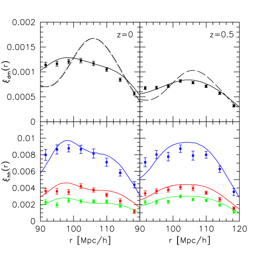
Figure 9 compares our model for the nonlinear correlation function, Eq. (51), with our measurements of (real-space) $\xi$ for the dark matter (top) and halos (bottom) at $z=0$ (left) and $z=0.5$ (right). The halo measurements are the same as those presented previously, except that now we only show scales which are within $\sim 15\,h^{-1}\,{\rm Mpc}$ of the initial acoustic peak.

Our model for the dark matter, Eq. (28), matches the measurements rather well; the solid lines are a substantial improvement over linear theory (dashed). Our model predicts that the peak has shifted to $105\,h^{-1}\,{\rm Mpc}$ by $z=0.5$, about a one percent effect; this is in good agreement with a more rigorous calculation based on RPT Crocce & Scoccimarro (2007). By $z=0$ our model for $\xi_{\rm dm}$ predicts that the peak has shifted to $98\,h^{-1}\,{\rm Mpc}$, roughly an $\sim 8$ percent shift! This disagrees by over a factor of four with the RPT calculation (apparent and physical shifts included); this overshoot is not surprising, when given the fact that one-loop PT is known to overestimate the nonlinear power spectrum by tens of percent on small scales, even though the one-loop density-velocity divergence power spectrum does well at reproducing the cross-power spectrum as measured from numerical simulations at intermediate scales Scoccimarro (2004).

Turning now to the results for the dark matter halos, we see that Eq. (51) provides a very good description of the measurements. We emphasize that there are no free parameters in this model. The only non-cosmological parameters in the model are the bias factors and as discussed earlier, these are measured directly from the simulations to make the predictions (see Section III.2 for our estimated values for the halo mass bins listed in Table 1).

When the bias factor is large, then the dominant nonlinear correction comes from $\Theta_{3}$ because it scales as $b^{2}$. For the dark matter, the nonlinear correction coming from $\Theta_{2}^{\rm 1loop}$ is the dominant one. The figure shows that our model does not predict any significant trend with halo mass, although this would likely change if we were to include nonlinear bias (e.g. Smith, Scoccimarro & Sheth (2007) suggest higher mass halos will show enhanced nonlinear effects). Our model requires knowledge of how these nonlinear bias terms evolve (i.e., the analog of Eq. 48): this evolution is given in Scoccimarro et al. (2001); Cooray & Sheth (2002).

V Conclusions

We have used analytic methods and a very large ensemble of numerical simulations to study how the position of the baryonic acoustic peak in the two-point correlation function, $\xi$, remnant of the tight coupling between photons and baryons before recombination, is affected by the clustering systematics: nonlinear mass evolution, bias and redshift space distortions; and we have examined these effects as a function of cosmological epoch and as a function of several trace particle types – i.e. halo samples picked to evolve with constant comoving number density.

We have investigated a toy-model for the evolution of $\xi$ (Sec II) that was simply a Gaussian bump plus a power-law and we showed that, if nonlinear evolution was manifest as a Gaussian smoothing of the true $\xi$, then the acoustic scale was not well recovered through simply measuring the local maximum – and this we described as an apparent shift of the peak. However, if there was a change in the underlying broad band power then this we said would lead to a a physical motion of the peak.

We presented results from our numerical simulations (Sec III.1). Our total simulated volume corresponded to $\sim~{}105~{}{\rm Gpc}^{3}h^{-3}$, approximately the same size volume that the proposed Stage IV, JDEM mission, ADEPT intends to surveyBennett et al. (2006). Therefore our results and analysis are of direct relevance to that and similar missions. From these simulations we measured $\xi$ for the dark matter and haloes. We found, at $z=0$ in both real and redshift space, that the true position and shape of the linear theory function did not match well that of the measured data – there being an enhanced signal on scales smaller than the unperturbed peak scale.

We then performed a more careful analysis, and fitted the correlation function data using the Gaussian smoothed linear theory model. This provided a much improved fit. In all cases the inferred peak positions from these models were shifted to smaller scales, with typical shifts being of the order $\sim 0.5-3.0~{}h^{-1}\,{\rm Mpc}$ – including a factor of $\sim 2$ correction for the transfer function; the shifts were enhanced for the the highest mass haloes/rarest objects and in redshift space. However they were alleviated for higher redshifts. We concluded that this was direct evidence for ‘apparent motion’ of the acoustic peak. We also noted that many of the recently proposed BAO reconstruction methods do attempt to account for this apparent shifting of the peak.

We then showed that the smoothed linear model was not a perfect fit to the data, in particular for highly biased haloes and their galaxies the fit was poor. Using the $\chi^{2}$ test we ruled out this model at the 99% significance. Furthermore, through inspection of the residuals of the fitting we found $\sim 10-20\%$ excess of amplitude on scales smaller than the unperturbed acoustic scale. We concluded that this was supporting evidence for the hypothesis that non-linear evolution was inducing a physical motion of the acoustic peak. We characterized the physical shifts by finding the local maximum of smooth polynomial fit to the data and subtracting from it the linear model peak position. We found that these shifts were of the order $\sim 0.0-3.0~{}h^{-1}\,{\rm Mpc}$ for the samples considered. We noted that these – which represent broad band tilting plus the more pernicious mode coupling effects – are not accounted for in recently proposed schemes to correct the signal in the power-spectrum.

In our analysis of the simulation data we also presented evidence that the simple Gaussian-based calculation for the variance (Eq. 13) of $\xi$ that included the Poisson shot-noise contribution provided a good description of the expected error on the measured $\xi$ for haloes (Figs. 4 and 5). In detail the Gaussian error model was found to underestimate the simulations for haloes at the present day. Adding non-Gaussian terms from the trispectrum and bispectrum may improve this further.

For future BAO missions that aim to use the power spectrum of clusters, the expected sample variance estimates that use the Gaussian plus Poisson model, will give reasonable estimates of the variance. Directly extrapolating our analysis to make a statement about the variance estimates for BAO galaxy surveys is complicated. Our analysis has dealt with the clustering of the halo centers and does not include the virial motions of particles/galaxies internal to the halo – adding in this layer of reality may lead to increased variance. Furthermore, if galaxies appear only in haloes, then using the galaxy number density estimate as the Poisson shot noise error as is common practice, will underestimate the sample variance when there is more than one galaxy per halo. We expect that the effective number density of the haloes that host the galaxies in the survey will be a better reflection of the errors. We shall reserve this issue for future study.

We then presented an analytic model that was able to capture the main observed affects from the non-linear evolution of the mass and bias. The model was based upon a study of the gravitationally driven mean streaming motions of particle pairs. These motions both smooth out the initial peak, and, more importantly, shift it (Fig. 7). In essence, our model simultaneously accounts for both the smoothing and the shifting of the acoustic peak. We first discussed the model in the context of the dark matter (Eq. 28), and then showed how it could be extended to describe the nonlinear evolution of $\xi$ for biased tracers, such as galaxies and clusters of galaxies as well (Eq. 51). For the dark matter, our approach is less reliable than that of RPT (see Crocce & Scoccimarro (2007) for a discussion of this). However, we think it has substantial merit, owing to the fact that it permits a simple description of how the shifting of the acoustic peak is modified for biased tracer particles. It also allows us to see the problem from a different perspective. One could combine the strength of both methods, by replacing the modeling of the divergence of pairwise velocities by its RPT description, for that one would need to calculate the bispectrum contribution to $\Theta_{3}$.

The measured shifts in the acoustic peak position for the dark matter and the biased tracers, are qualitatively consistent with the effects of the clustering systematics on the power spectrum Smith, Scoccimarro & Sheth (2007). This owes to the fact that the power spectrum and correlation functions are a Fourier transform pair. Thus small scale damping and tilting of the linear power spectrum can lead to both smoothing and tilting of the correlation function, and the generation of the measured apparent and physical motion of the peak.

However, these recovered shift values appear substantially larger than those currently quoted in the literature from other analytic arguments Eisenstein, Seo & White (2006). One possible explanation for this is that the divergence of the pairwise velocity field is substantially more non-linear than the density field on these large scales (Fig. 8). Had we simply used linear theory velocities in our analytic model then we would have considerably underestimated the measured shifts. Using perturbation theory was crucial (Eqs. 43–47) for our model to get the close agreement with the numerical measurements.

If unaccounted for, the percent level changes we have measured in the acoustic scale will lead to biased determinations of cosmological parameters (and see Angulo et al. (2007)). However, the agreement between our model and the simulations suggests that, although such pernicious shifts are present, it may be possible to construct analytic tools that allow us to correct for them. This is the subject of ongoing work.

Appendix A The Divergence of Infall velocities in Perturbation Theory

This Appendix provides expressions for $\Theta_{2}^{\rm 1loop}(r)$ and $\Theta_{3}(r)$ from the standard PT.

A.1 $\Theta_{2}^{\rm 1loop}$ in the standard PT

$\Theta_{2}^{\rm 1loop}$ is given by Eqs. (44) and (45), and is an integral over the 1-Loop contribution to the velocity divergence-density power spectrum. In the standard Perturbation Theory this can be written Scoccimarro (2004):

$$P^{\delta\theta}_{\rm 1loop}(k)=2\int F_{2}({\hbox{\BF k}}-{\hbox{\BF q}},{\hbox{\BF q}})\,G_{2}({\hbox{\BF k}}-{\hbox{\BF q}},{\hbox{\BF q}})\,P_{0}(|{\hbox{\BF k}}-{\hbox{\BF q}}|)\,P_{0}(q)\,d^{3}q+3\,P_{0}(k)\int[\hat{F}_{3}(k,q)+\hat{G}_{3}(k,q)]\,P_{0}(q)\,d^{3}q,$$ (53)

where the functions $F_{2}({\hbox{\BF k}},{\hbox{\BF q}})$ and $G_{2}({\hbox{\BF k}},{\hbox{\BF q}})$ are the second order, symmetric, density and velocity divergence kernels from PT Bernardeau et al. (2002). These are written:

$$F_{2}({\hbox{\BF k}},{\hbox{\BF q}}) = \frac{5}{7}+\frac{1}{2}\,\mu_{k,q}\,\Big{(}\frac{k}{q}+\frac{q}{k}\Big{)}+\frac{2}{7}\,\mu_{k,q}^{2}\ ;$$ (54)

$$G_{2}({\hbox{\BF k}},{\hbox{\BF q}}) = \frac{3}{7}+\frac{1}{2}\,\mu_{k,q}\,\Big{(}\frac{k}{q}+\frac{q}{k}\Big{)}+\frac{4}{7}\,\mu_{k,q}^{2}\ ,$$ (55)

where $\mu_{k,q}\equiv{\hbox{\BF k}}\cdot{\hbox{\BF q}}/|k||q|$. The functions $\hat{F}_{3}(k,q)$ and $\hat{G}_{3}(k,q)$ are the angle averages of the third order PT density and velocity kernels. These may be written:

$$\hat{F}_{3}(k,q) = \int\frac{d\hat{q}}{4\pi}F_{3}({\hbox{\BF k}},{\hbox{\BF q}},-{\hbox{\BF q}})=\frac{1}{24}\left[\frac{6k^{6}-79k^{4}q^{2}+50k^{2}q^{4}-21q^{6}}{63k^{2}q^{4}}+\frac{(q^{2}-k^{2})^{3}(7q^{2}+2k^{2})}{42k^{3}q^{5}}\ \ln\Big{|}\frac{k+q}{k-q}\Big{|}\right]\ ;$$ (56)

$$\hat{G}_{3}(k,q) = \int\frac{d\hat{q}}{4\pi}G_{3}({\hbox{\BF k}},{\hbox{\BF q}},-{\hbox{\BF q}})=\frac{1}{24}\left[\frac{6k^{6}-41k^{4}q^{2}+2k^{2}q^{4}-3q^{6}}{21k^{2}q^{4}}+\frac{(q^{2}-k^{2})^{3}(q^{2}+2k^{2})}{14k^{3}q^{5}}\ \ln\Big{|}\frac{k+q}{k-q}\Big{|}\right]\ .$$ (57)

A.2 $\Theta_{3}(r)$ in the standard PT

$\Theta_{3}(r)$ is related to the density-velocity divergence-density bispectrum through two Fourier transforms (Eq. 47). In the standard PT this bispectrum is:

$$B^{\delta\theta\delta}({\hbox{\BF k}}_{1},{\hbox{\BF k}}_{2},{\hbox{\BF k}}_{3})=2F_{2}({\hbox{\BF k}}_{2},{\hbox{\BF k}}_{3})P_{0}(k_{2})P_{0}(k_{3})+2G_{2}({\hbox{\BF k}}_{1},{\hbox{\BF k}}_{3})P_{0}(k_{1})P_{0}(k_{3})+2F_{2}({\hbox{\BF k}}_{1},{\hbox{\BF k}}_{2})P_{0}(k_{1})P_{0}(k_{2})\ .$$ (58)

In order to proceed we require some further pieces of information. Firstly, the closure relation for $k$-modes gives us ${\hbox{\BF k}}_{3}=-{\hbox{\BF k}}_{1}-{\hbox{\BF k}}_{2}$. Secondly, statistical homogeneity and isotropy means that the bispectrum can be written as a function of three variables: the length of two sides of a triangle and the angles between them, i.e. we should at the end of our calculation be able to write $B^{\delta\theta\delta}({\hbox{\BF k}}_{1},{\hbox{\BF k}}_{2},{\hbox{\BF k}}_{3})\equiv B^{\delta\theta\delta}(k_{1},k_{2},\theta_{12})$. Thirdly, the addition theorem for spherical harmonics allows us to re-write the angles between any two vectors in terms of their own angles in some arbitrary Cartesian system:

$$\cos\theta_{12}=\cos\theta_{1}\cos\theta_{2}+\sin\theta_{1}\sin\theta_{2}\cos(\phi_{1}-\phi_{2})\ ,$$ (59)

where the angle between the two vectors ${\hbox{\BF k}}_{1}~{}\{k_{1},\theta_{1},\phi_{1}\}$ and ${\hbox{\BF k}}_{2}~{}\{k_{2},\theta_{2},\phi_{2}\}$ is $\theta_{12}$. Some lengthy algebra then leads us to the following expression for $\Theta_{3}(r)$:

$$\Theta_{3}(r) = 2\Bigg{[}\int d^{3}k\,P_{0}(k)\,j_{1}(kr)\,k\int d^{3}q\,P_{0}(q)\Big{[}\Big{(}\frac{q}{k}{\hat{{\hbox{\BF k}}}}\cdot{\hat{{\hbox{\BF q}}}}+1\Big{)}\frac{2G_{2}({\hbox{\BF k}},{\hbox{\BF q}})}{|{\hbox{\BF k}}+{\hbox{\BF q}}|^{2}}-\frac{1}{3}\Big{(}\frac{1}{q^{2}}+\frac{1}{k^{2}}\Big{)}\Big{]}+\frac{34}{21}\Psi_{0}^{0}(r)\Psi_{1}^{-1}(r)$$ (60)

$$-\frac{2}{3}\Big{[}\Psi_{2}^{0}(r)\Psi_{1}^{-1}(r)+\Psi_{2}^{-2}(r)\Psi_{1}^{1}(r)\Big{]}+\frac{1}{3}\Big{[}\Psi_{0}^{0}(r)\Psi_{1}^{-1}(r)+\Psi_{0}^{-2}(r)\Psi_{1}^{1}(r)\Big{]}+\frac{8}{35}\Psi_{2}^{0}(r)\Psi_{3}^{-1}(r)$$

$$-\frac{16}{105}\Psi_{2}^{0}(r)\Psi_{1}^{-1}(r)\Bigg{]}\ ,$$

where we have introduced the useful auxiliary function

$$\Psi_{\ell}^{m}(r)=\int d^{3}q\,P_{0}(q)\,j_{\ell}(qr)\,q^{m}\ .$$ (61)

References

- Spergel et al. (2006) D. Spergel, & The WMAP Team, astro-ph/0603449 (2006).
- Tegmark et al. (2006) M. Tegmark, M. & The SDSS Team, astro-ph/0608632 (2006).
- S nchez et al. (2006) A. G. S nchez, C. M. Baugh, W. J. Percival, J. A. Peacock, N. Padilla, S. Cole, C. S. Frenk, P. Norberg, Mon. Not. R. Astron. Soc. , 366, 189 (2006).
- Astier et al. (2006) P. Astier, & The Super Nova Legacy Survey Team, A&A, 447, 31-48 (2006).
- Hoekstra et al. (2006) H. Hoekstra, & The CFHTLS Team, ApJ, 647, 116 (2006).
- Cole et al. (2005) S. Cole, & The 2dfGRS Team, Mon. Not. R. Astron. Soc. , 362, 505 (2005).
- Eisenstein et al. (2005) D. J. Eisenstein et al., Astrophys. J. 633, 560 (2005).
- Peebles & Ratra (2003) J. P. Peebles, B. Ratra, Rev. Mod. Phys. , 75 559 (2003).
- DETF (2006) A. Albrecht, G. Bernstein, R. Cahn, W. L. Freedman, J. Hewitt, W. Hu, J. Huth, M. Kamionkowski, E. Kolb, L. Knox, J. Mather, S. Staggs, N. Suntzeff, “Dark Energy Task Force Report for NSF and DOE”, astro-ph/0609591 (2006).
- ESO (2006) J. A. Peacock, P. Schneider, G. Efstathiou, J. R. Ellis, B. Leibundgut, S. J. Lilly, Y. Mellier, “ESA-ESO Working Groups Report on Fundamental Cosmology”, astro-ph/0610906 (2006).
- Angulo et al. (2007) R. Angulo, C. M. Baugh, C. S. Frenk, C. G. Lacey, Mon. Not. R. Astron. Soc. , submitted astro-ph/0702543 (2007).
- Hinshaw et al. (2006) G. Hinshaw, & The WMAP Team, astro-ph/0603451 (2006).
- Eisenstein & Hu (1998) D. J. Eisenstein, W. Hu, Astrophys. J. , 496, 605 (1998).
- Percival et al. (2001) W. Percival et al., Mon. Not. R. Astron. Soc. , 327 1297 (2001).
- Tegmark et al. (2004) M. Tegmark et al., Astrophys. J. 606, 702 (2004).
- Percival et al. (2007a) W. Percival et al., Astrophys. J. , 657, 645, (2007a).
- Percival et al. (2007b) W. Percival et al.,Astrophys. J. , 657, 51, (2007b).
- Hutsi (2006a) G. Hütsi, A&A, 449, 891 (2006a).
- Hutsi (2006b) G. Hütsi, A&A, 459, 375 (2006b).
- Padmanabhan et al. (2006) N. Padmanabhan, & The SDSS Team, astro-ph/0605302 (2006).
- Meiskin, White & Peacock (1999) A. Meiksin, M. White, J. A. Peacock, Mon. Not. R. Astron. Soc. , 304, 851 (1999).
- Blake & Glazebrook (2003) C. Blake, K. Glazebrook, Astrophys. J. , 594, 665 (2003).
- Seo & Eisenstein (2005) H.-J. Seo, D. Eisenstein, Astrophys. J. , 633, 575 (2005).
- White (2005) M. White, Astro-particle Phys. , 24, 334 (2005).
- Angulo et al. (2005) R. Angulo, C. M. Baugh, C. S. Frenk, R. G. Bower, A. Jenkins, S. Morris Mon. Not. R. Astron. Soc. , 362, 25 (2005).
- Springel et al. (2005) V. Springel, et al., Nature (London) , 435, 629 (2005).
- Dolney, Jain & Takada (2006) D. Dolney, B. Jain, M. Takada, Mon. Not. R. Astron. Soc. , 366, 884 (2006).
- Huff et al. (2006) E. Huff, A. E. Schulz, M. White, D. J. Schlegel, M. Warren, astro-ph/0607061 (2006).
- Bernstein (2006) G. Bernstein, Astrophys. J. , 637, 598 (2006).
- Eisenstein, Seo & White (2006) D. J. Eisenstein, H.-J. Seo, M. White, Astrophys. J. , submitted, astro-ph/0604361 (2006).
- Bharadwaj (1996) S. Bharadwaj, Astrophys. J. , 472, 1 (1996)
- Eisenstein et al. (2006) D. J. Eisenstein, H. J. Seo, E. Sirko, D. Spergel, Astrophys. J. , submitted, astro-ph/0604362 (2006).
- Jeong & Komatsu (2006) D. Jeong, E. Komatsu, astro-ph/0604075 (2006).
- Wang (2006) Y. Wang, Astrophys. J. , 647, 1 (2006).
- Smith, Scoccimarro & Sheth (2007) R. E. Smith, R. Scoccimarro, R. K. Sheth, Phys. Rev. D. , 75, 063512 (2007).
- Ma (2007) Z. Ma, astro-ph/0610213 (2007).
- Crocce & Scoccimarro (2007) M. Crocce, R. Scoccimarro, arXiv:0704.2783 (2007).
- Matarrese & Pietroni (2007) S. Matarrese, M. Pietroni, astro-ph/0702653 (2007).
- Guzik, Bernstein & Smith (2007) J. Guzik, G. Bernstein, R. E. Smith, Mon. Not. R. Astron. Soc. , 375, 1329 (2007).
- Smith et al. (2003) R. E. Smith, J. A. Peacock, A. Jenkins, S. D. M. White, C. S. Frenk, F. R. Pearce, P.A. Thomas, G. Efstathiou H. M. P. Couchman, Mon. Not. R. Astron. Soc. 341, 1311 (2003).
- Crocce & Scoccimarro (2006a) M. Crocce, R. Scoccimarro, Phys. Rev. D. 73, 063519 (2006).
- Crocce & Scoccimarro (2006b) M. Crocce, R. Scoccimarro, Phys. Rev. D. 73, 063520 (2006).
- Bennett et al. (2006) C. Bennett, Space Studies Board, National Academies, www7.nationalacademies.org/ssb/BE_Nov_2006_bennett.pdf, (2006).
- Seljak & Zaldarriaga (1996) U. Seljak, M. Zaldarriaga, Astrophys. J. 469, 437 (1996).
- Scoccimarro (1998) R. Scoccimarro, Mon. Not. R. Astron. Soc. , 299, 1097 (1998).
- Crocce et al. (2006) M. Crocce, S. Pueblas, R. Scoccimarro, Mon. Not. R. Astron. Soc. , 373, 369 (2006).
- Springel (2005) V. Springel, Mon. Not. R. Astron. Soc. , 364, 1105 (2005).
- Warren et al. (2005) M. S. Warren, K. Abazajian, D. E. Holz, L. Teodoro, astro-ph/0604310 (2005).
- Bernstein (1994) G. M. Bernstein, Astrophys. J. 424, 569 (1994).
- Cohn (2006) J. D. Cohn, New Astronomy 11, 226 (2006).
- Feldman, Kaiser & Peacock (1994) H. Feldman, N. Kaiser, J. A. Peacock, Astrophys. J. , 426, 23 (1994).
- Scoccimarro, Zaldarriaga & Hui (1999) R. Scoccimarro, M. Zaldarriaga, L. Hui, Astrophys. J. , 527, 1 (1999).
- Meiksin & White (1999) A. Meiksin, M. White, Mon. Not. R. Astron. Soc. , 308, 1179 (1999).
- Neyrink & Szapudi (2007) M. Neyrink, I. Szapudi, Mon. Not. R. Astron. Soc. submitted, astro-ph/0710.3586 (2007).
- Press et al. (1992) W. Press, S. Teukolsky, W. Vetterling, B. Flannery, “Numerical recipes in Fortran 77”, 1992, Cambridge University Press, Cambridge, England.
- Schulz & White (2006) A. E. Shulz, M. White, Astro-particle Phys. , 25, 172 (2006).
- Bernardeau et al. (2002) F. Bernardeau, S. Colombi, E. Gaztañga, R. Scoccimarro, Physics Reports 367, 1 (2002).
- Peebles (1980) P.J.E. Peebles, 1980, The large-scale structure of the universe, Princeton University Press, Princeton, NJ.
- Nityananda & Padmanhbhan (1994) R. Nityananda, T. Padmanhbhan, Mon. Not. R. Astron. Soc. , 271, 976 (1994).
- Fisher (1995) K. B. Fisher, Astrophys. J. , 448, 494 (1995).
- Juszkiewicz et al. (1999) R. Juszkiewicz, V. Springel, R. Durrer, Astrophys. J. Lett. , 518, L25 (1999).
- Landau & Lifschitz (1959) L. Landau, E. M. Lifschitz, “Course of Theoretical Physics, Vol. 6 Fluid Mechanics”, Pergamon Press Ltd, Oxford, England (1959).
- (63) In solving equations like , we assume that the velocity field is curl free, whence and thus . This may be solved most simply in Fourier space: .
- Coles & Jones (1991) P. Coles, B. J. T. Jones, Mon. Not. R. Astron. Soc. , 248, 1 (1991).
- Hamilton et al. (1991) A. J. S. Hamilton, P. Kumar, E. Lu, A. Matthews, Astrophys. J. Lett. , 374, L1 (1991).
- Scoccimarro (2004) R. Scoccimarro, Phys. Rev. D. , 70, 083007 (2004).
- Sheth et al. (2001) R. K. Sheth, A. Diaferio, L. Hui, R. Scoccimarro, Mon. Not. R. Astron. Soc. , 326, 463 (2001).
- Nusser & Davis (1994) A. Nusser, M. Davis, Astrophys. J. Lett. , 421, L1 (1994).
- Mo & White (1996) H. J. Mo, S. D. M. White, Mon. Not. R. Astron. Soc. , 282, 347 (1996).
- Fry (1996) J. N. Fry, Astrophys. J. Lett. , 461, L65 (1996).
- Tegmark & Peebles (1998) M. Tegmark, P. J. E. Peebles, Astrophys. J. Lett. , 500, L79 (1998).
- Sheth & Tormen (1999) R. K. Sheth, G. Tormen, Mon. Not. R. Astron. Soc. , 308, 119 (1999).
- Scoccimarro et al. (2001) R. Scoccimarro, R. K. Sheth, L. Hui, B. Jain, Astrophys. J. , 546, 20 (2001).
- Cooray & Sheth (2002) A. Cooray, R. K. Sheth, Phys. Rep. , 372, 1 (2002).