Analytic spectrum of relic gravitational waves modified by neutrino free streaming and dark energy

We include the effect of neutrino free streaming into the spectrum of relic gravitational waves (RGWs) in the currently accelerating universe. For the realistic case of a varying fractional neutrino energy density and a non-vanishing derivative of mode function at the neutrino decoupling, the integro-differential equation of RGWs is solved by a perturbation method for the period from the neutrino decoupling to the matter-dominant stage. Incorporating it to the analytic solution of the whole history of expansion of the universe, the analytic solution of GRWs is obtained, evolving from the inflation up to the current acceleration. The resulting spectrum of GRWs covers the whole range of frequency $(10^{-19}\sim 10^{10})$Hz, and improves the previous results. It is found that the neutrino free-streaming causes a reduction of the spectral amplitude by $\sim 20\%$ in the range $(10^{-16}\sim 10^{-10})$ Hz, and leaves the other portion of the spectrum almost unchanged. This agrees with the earlier numerical calculations. Examination is made on the difference between the accelerating and non-accelerating models, and our analysis shows that the ratio of the spectral amplitude in accelerating $\Lambda$CDM model over that in CDM model is $\sim 0.7$, and within the various accelerating models of $\Omega_{\Lambda}>\Omega_{m}$ the spectral amplitude is proportional to $\Omega_{m}/\Omega_{\Lambda}$ for the whole range of frequency. Comparison with LIGO S5 Runs Sensitivity shows that RGWs are not yet detectable by the present LIGO, and in the future LISA may be able to detect RGWs in some inflationary models.

PACS numbers: 04.30.-w, 98.80.-k, 04.62.+v

1. Introduction

Inflationary models generally predict the existence of a stochastic background of relic gravitational waves (RGWs). [1, 2, 3]. Due to their very weak coupling with matter, RGWs still encode a wealth of information about the very early universe when they were generated, and enable us to study the inflationary and the successive physical processes, much earlier than the recombination time at a temperature $T\sim 0.3$ ev, up to which CMB information can tell. Not only the RGWs are the scientific goal of the detections, such as the laser interferometers now underway [4, 5, 6, 7], but also are a source, along with the density perturbations, of CMB anisotropies and polarizations [8, 9, 10, 11, 12, 13]. In particular, the B-polarization of CMB can only be generated by RGWs. Thus, it is important to calculate the spectrum of RGWs, which depends on several physical processes. First of all, it depends sensitively on the specific inflationary models [1, 3]. Moreover, after being generated, the spectrum of RGWs can be further modified by the subsequent expansion of the universe, giving rise to the redshift-suppression on the spectrum. In our previous analytic and numerical investigations [3], we studied the RGWs in the current accelerating expansion of the universe, obtained the modifications on the spectrum by the presence of dark energy. In particular, we have found that the amplitude of RGWs is reduced by a factor $\sim 0.3$ in comparison with the matter-dominant models, and that within the $\Lambda$CDM models with $\Omega_{\Lambda}>\Omega_{m}$, the amplitude $\propto\Omega_{m}/\Omega_{\Lambda}$, over almost the whole frequency range of the spectrum.

There are other processes that can also change the spectrum of RGWs. One important process is the free-streaming of neutrinos that occurred in the early universe [14]. It will leave the imprints on the spectrum. At a temperature $T\sim 2$ Mev during the radiation-dominant stage in the early universe, cosmic neutrinos decoupled from electrons and photons, and started free-streaming in space. This will give rise to an anisotropic part $\pi_{ij}$ of the energy-momentum tensor $T_{ij}$ as a source of the equation of RGWs, and will cause a damping effect on the RGWS. Weinberg analyzed the effect and arrived at the integro-differential equation for RGWs, and gave an estimate of the damping on RGWs due to the neutrinos free-streaming [14]. Subsequently, in the special case of a constant fractional neutrino energy density $f_{\nu}(0)$, a vanishing time $u_{dec}=0$ of the neutrino decoupling, and a vanishing time-derivative $\chi^{\prime}(u_{dec})=0$, Dicus and Repko [15] obtained an analytic solution, in terms of a series of Bessel’s functions, of the integro-differential equation for the radiation stage, qualitatively agreeing with Weinberg’s estimate. However, this solution holds only for the short wavelength modes reentering the horizon long after the neutrino decoupling during radiation-dominant stage, and the conditions it has used are actually approximations and will obviously cause some errors. Moreover, as Weinberg points out, the solution for the radiation stage is still to be joined with those for other expansion stages, so that the effect of neutrino free streaming is taken into account in a complete computation of the spectrum of RGWs. In a numerical study of the matter-dominant universe, Watanabe and Komatsu [16] investigated the damping effects on the RGWs caused by the evolution of the effective relativistic degrees of freedom, including the neutrino free-streaming, and gave a numerical solution of the energy density spectrum [16]. But there the important effect of the acceleration of the present universe has not been considered.

In this paper, extending our previous work on the analytic spectrum of RGWs in the accelerating universe [3], we will include the damping effect of neutrino free-streaming into our analytic calculation scheme. Both effects of the accelerating universe and of the neutrino free streaming are taken into account, simultaneously. The following improvements are achieved in this paper over the previous studies. In comparison with Ref.[16], the damping effect on the spectrum of RGWs by the dark energy $\Omega_{\Lambda}$ is now properly included. Different from Dicus and Repko’s method of series expansion that is valid in the special case [15], we apply a perturbation method to solve the integro-differential equation of RGWs by an iterative procedure. Actually, for practical use, the first order solution is enough for an evaluation for the spectrum of RGWs, and the solution of higher accuracy can be easily achieved by going to higher order of iterations. This calculation has the merit of precisely taking into account of the time-varying fractional neutrino energy density $f_{\nu}(u)$, the non-vanishing time $u_{dec}\neq 0$ and the non-vanishing time-derivative $\chi^{\prime}(u_{dec})\neq 0$ of the mode functions. Therefore, the result is valid for all the modes of RGWs of an arbitrary wavelength, and reduces to that in Ref.[15] in the special case for the short wave length limit. We give the analytic expressions of the full spectrum $h(k,\eta_{H})$ of RGWs itself and of the spectral energy density $\Omega_{g}(k)$, valid for the whole range of frequencies. As a comprehensive compilation, by using the parameters $\beta$, $\beta_{s}$, $\gamma$ and $r$, respectively, such important cosmological elements have been explicitly parameterized, as the inflation, the reheating, the dark energy, the tensor/scalar ratio. This will considerably facilitate further studies on the RGWs and the relevant physical processes. Besides, several typographical errors in the previous studies have been corrected thereby. So not only can it be easily used in computation for other applications in cosmology, such as calculations of CMB anisotropies and polarizations generated by RGWs [12], but also can be directly compared with the sensitivity curves of those ongoing and forthcoming laser interferometer GW detectors, such as LIGO, LISA, etc [4, 5, 6, 7].

The outline of this paper is as follows. In section 2, to various stages of expansion of the universe the scale factor $a(\eta)$ is specified with the parameters being determined by the continuity conditions. In section 3, we present the analytical solutions of the modes $h_{k}(\eta)$ of RGWs during each stage, and, in particular, include the effect of neutrino free streaming during the radiation-dominant stage. The subtleties of interpreting the observational data within the non-accelerating models are discussed. In section 4, we present the resulting spectrum and analyze the effects of $\beta,\beta_{s},\gamma$, $r$ and the neutrino free streaming. The Appendix gives the detailed calculation of the anisotropic part $\pi_{ij}$ of the energy-momentum tensor, and present the perturbation method for the solution modified by the neutrino free-streaming during the radiation stage. In this paper we use unit with $c=\hbar=k_{B}=1$.

2. Expansion history of the universe

From the inflationary up to the current accelerating stage, the expansion of a spatially flat universe can be described by the spatially flat ($\Omega_{\Lambda}+\Omega_{m}+\Omega_{r}=1$) Robertson-Walker spacetime with a metric

$$ds^{2}=a^{2}(\eta)[-d\eta^{2}+\delta_{ij}dx^{i}dx^{j}],$$ (1)

where the scale factor has the following forms for the successive stages [17]:

The inflationary stage:

$$a(\eta)=l_{0}|\eta|^{1+\beta},\,\,\,\,-\infty<\eta\leq\eta_{1},$$ (2)

where $1+\beta<0$, and $\eta_{1}<0$. The special case of $\beta=-2$ is the de Sitter expansion of inflation.

The reheating stage:

$$a(\eta)=a_{z}|\eta-\eta_{p}|^{1+\beta_{s}},\,\,\,\,\eta_{1}\leq\eta\leq\eta_{s},$$ (3)

here we take the absolute value of $\eta-\eta_{p}$, different from Ref. [3]. This is because $1+\beta_{s}$ might be negative for some models of the reheating. As a model parameter, we will mostly take $\beta_{s}=-0.3$, though other values are also taken to demonstrate the effect of the various reheating models.

The radiation-dominant stage:

$$a(\eta)=a_{e}(\eta-\eta_{e}),\,\,\,\,\eta_{s}\leq\eta\leq\eta_{2}.$$ (4)

This is the stage during which the neutrinos decoupled from the radiation component. We use $\eta_{dec}$ to denote the starting time of the neutrino decoupling: $\eta_{s}<\eta_{dec}<\eta_{2}$. The corresponding energy scale is $\sim 2$ Mev for the decoupling. As will be seen later, the wave equation of RGWs is still homogeneous for $\eta<\eta_{dec}$, but becomes inhomogeneous for $\eta_{dec}<\eta<\eta_{2}$.

The matter-dominant stage:

$$a(\eta)=a_{m}(\eta-\eta_{m})^{2},\,\,\,\,\eta_{2}\leq\eta\leq\eta_{E}.$$ (5)

The accelerating stage up to the present time $\eta_{H}$ [3]:

$$a(\eta)=l_{H}|\eta-\eta_{a}|^{-\gamma},\,\,\,\,\eta_{E}\leq\eta\leq\eta_{H},$$ (6)

where the index $\gamma$ depends on the dark energy $\Omega_{\Lambda}$. By numerically solving the Friedmann equation [3],

$$(\frac{a^{\prime}}{a^{2}})^{2}=\frac{8\pi G}{3}(\rho_{\Lambda}+\rho_{m}+\rho_{r}),$$ (7)

where $a^{\prime}\equiv da/d\eta$, we find that $\gamma\simeq 1.06$ for $\Omega_{\Lambda}=0.65$, $\gamma\simeq 1.05$ for $\Omega_{\Lambda}=0.7$, and $\gamma\simeq 1.044$ for $\Omega_{\Lambda}=0.75$ (as a correction to $\gamma\simeq 1.048$ in Ref.[3]).

In the above specifications of $a(\eta)$, there are five instances of time, $\eta_{1}$, $\eta_{s}$, $\eta_{2}$, $\eta_{E}$, and $\eta_{H}$, which separate the different stages. Four of them are determined by how much $a(\eta)$ increases over each stage by the cosmological considerations. We take the following specifications: $\zeta_{1}=\frac{a(\eta_{s})}{a(\eta_{1})}=300$ for the reheating stage, $\zeta_{s}=\frac{a(\eta_{2})}{a(\eta_{s})}=10^{24}$ for the radiation stage, $\zeta_{2}=\frac{a(\eta_{E})}{a(\eta_{2})}=\frac{a(\eta_{H})}{a(\eta_{2})}\frac{a(\eta_{E})}{a(\eta_{H})}=3454\zeta_{E}^{-1}$ for the matter stage, and $\zeta_{E}=\frac{a(\eta_{H})}{a(\eta_{E})}=(\frac{\Omega_{\Lambda}}{\Omega_{m}})^{1/3}$ for the present accelerating stage. Note that here $(\frac{\Omega_{\Lambda}}{\Omega_{m}})^{1/3}$ is model-dependent, and associated with the value of $\gamma$, instead of the fixed value (1.33, as in Ref.[3]). The remaining time instance is fixed by an overall normalization, namely

$$|\eta_{H}-\eta_{a}|=1.$$ (8)

There are twelve constants in the expressions of $a(\eta)$, among which $\beta$, $\beta_{s}$ and $\gamma$ are imposed as the model parameters, for the inflation, the reheating, and the acceleration, respectively. So there remain nine constants. By the continuity of $a(\eta)$ and of $a(\eta)^{\prime}$ at the four given joining points $\eta_{1}$, $\eta_{s}$, $\eta_{2}$ and $\eta_{E}$, one can fix eight constants. Only one constant remains, which can be fixed by the present expansion rate $H_{0}$ of the universe and Eq.(8),

$$l_{H}=\gamma/H_{0}.$$ (9)

Then all parameters are fixed as the following:

$$\eta_{a}-\eta_{E}=\zeta_{E}^{\frac{1}{\gamma}},$$

$$\eta_{E}-\eta_{m}=\frac{2}{\gamma}\zeta_{E}^{\frac{1}{\gamma}},$$

$$\eta_{2}-\eta_{m}=\frac{2}{\gamma}\zeta_{2}^{-\frac{1}{2}}\zeta_{E}^{\frac{1}{\gamma}},$$

$$\eta_{2}-\eta_{e}=\frac{1}{\gamma}\zeta_{2}^{-\frac{1}{2}}\zeta_{E}^{\frac{1}{\gamma}},$$

$$\eta_{s}-\eta_{e}=\frac{1}{\gamma}\zeta_{s}^{-1}\zeta_{2}^{-\frac{1}{2}}\zeta_{E}^{\frac{1}{\gamma}},$$

$$\eta_{s}-\eta_{p}=\frac{1}{\gamma}(1+\beta_{s})\zeta_{s}^{-1}\zeta_{2}^{-\frac{1}{2}}\zeta_{E}^{\frac{1}{\gamma}},$$

$$\eta_{1}-\eta_{p}=\frac{1}{\gamma}(1+\beta_{s})\zeta_{1}^{\frac{-1}{1+\beta_{s}}}\zeta_{s}^{-1}\zeta_{2}^{-\frac{1}{2}}\zeta_{E}^{\frac{1}{\gamma}},$$

$$\eta_{1}=\frac{1}{\gamma}(1+\beta)\zeta_{1}^{\frac{-1}{1+\beta_{s}}}\zeta_{s}^{-1}\zeta_{2}^{-\frac{1}{2}}\zeta_{E}^{\frac{1}{\gamma}},$$

$$\eta_{dec}=1.15\times 10^{-10}\zeta_{E}\zeta_{2}\eta_{2},$$ (10)

and

$$a_{m}=\frac{l_{H}}{4}\,\gamma^{2}\,\zeta_{E}^{-(1+\frac{2}{\gamma})},$$

$$a_{e}=l_{H}\,\gamma\,\zeta_{2}^{-\frac{1}{2}}\zeta_{E}^{-(1+\frac{1}{\gamma})},$$

$$a_{z}=l_{H}\,\gamma^{1+\beta_{s}}|1+\beta_{s}|^{-(1+\beta_{s})}\zeta_{s}^{\beta_{s}}\zeta_{2}^{\frac{\beta_{s}-1}{2}}\zeta_{E}^{-(1+\frac{1+\beta_{s}}{\gamma})},$$

$$l_{0}=l_{H}\,\gamma^{1+\beta}\,|1+\beta|^{-(1+\beta)}\zeta_{1}^{\frac{\beta-\beta_{s}}{1+\beta_{s}}}\zeta_{s}^{\beta}\zeta_{2}^{\frac{\beta-1}{2}}\zeta_{E}^{-(1+\frac{1+\beta}{\gamma})}.$$ (11)

The above expressions correct some typographical errors in Ref.[3].

In the expanding universe, the physical wavelength is related to the comoving wavenumber $k$ by

$$\lambda\equiv\frac{2\pi a(\eta)}{k},$$ (12)

and the wavenumber $k_{H}$ corresponding to the present Hubble radius is

$$k_{H}=\frac{2\pi a(\eta_{H})}{1/H_{0}}=2\pi\gamma.$$ (13)

There is another wavenumber

$$k_{E}\equiv\frac{2\pi a(\eta_{E})}{1/H_{0}}=\frac{k_{H}}{1+z_{E}},$$ (14)

whose corresponding wavelength at the time $\eta_{E}$ is the Hubble radius $1/H_{0}$. In the present universe the physical frequency corresponding to a wavenumber $k$ is given by

$$\nu=\frac{1}{\lambda}=\frac{k}{2\pi a(\eta_{H})}=\frac{H_{0}}{2\pi\gamma}k.$$ (15)

3. Analytical solution

In the presence of the gravitational waves, the perturbed metric is

$$ds^{2}=a^{2}(\eta)[-d\eta^{2}+(\delta_{ij}+h_{ij})dx^{i}dx^{j}],$$ (16)

where the tensorial perturbation $h_{ij}$ is a $3\times 3$ matrix and is taken to be transverse and traceless

$$h^{i}_{\,\,i}=0, h_{ij,j}=0.$$ (17)

The wave equation of RGWs is

$$\partial_{\nu}(\sqrt{-g}\partial^{\nu}h_{ij})=0.$$ (18)

However, from the temperature $T\simeq 2$ Mev up to the beginning of the matter domination, the neutrinos are decoupled from electrons and photons and start to freely stream in space. This effect of neutrino free streaming gives rise to an anisotropic portion $\pi_{ij}$ of the energy-momentum stress $T_{ij}$. Then Eq.(18) acquires an inhomogeneous source term $-16\pi G\pi_{ij}$ on the right hand side during the period $\eta_{dec}<\eta<\eta_{2}$. As is shown in the Appendix, the anisotropic stress $\pi_{ij}$ is also transverse and traceless, and it is zero before the decoupling and becomes negligible small after the matter domination. To solve the equation, we decompose $h_{ij}$ into the Fourier modes of the comoving wave number $k$ and into the polarization state $\sigma$ as

$$h_{ij}(\eta,{\bf x})=\sum_{\sigma}\int\frac{d^{3}k}{(2\pi)^{3}}\epsilon^{\sigma}_{ij}h_{k}^{(\sigma)}(\eta)e^{i\bf{k}\cdot{x}}\,,$$ (19)

where $h_{-k}^{(\sigma)*}(\eta)=h_{k}^{(\sigma)}(\eta)$ ensuring that $h_{ij}$ be real, $\epsilon^{\sigma}_{ij}$ is the polarization tensor, and $\sigma$ denotes the polarization states $\times,+$. Here $h_{ij}$ is treated as a classical field, instead of a quantum operator [1, 3]. In terms of the mode $h^{(\sigma)}_{k}$, Eq.(19) reduces to

$$h^{(\sigma)}_{k}{{}^{\prime\prime}}(\eta)+2\frac{a^{\prime}(\eta)}{a(\eta)}h^{(\sigma)}_{k}{{}^{\prime}}(\eta)+k^{2}h^{(\sigma)}_{k}(\eta)=0.$$ (20)

Since for each polarization, $\times$, $+$, the wave equation is the same and has the same statistical properties, from now on the super index $(\sigma)$ can be dropped from $h^{(\sigma)}_{k}$. As demonstrated in Eq.(2) through Eq.(6), for all the stages of expansion the time-dependent scale factor is of a generic form

$$a(\eta)\propto\eta^{\alpha},$$ (21)

the solution to Eq.(20) is a linear combination of Bessel function $J_{\nu}$ and Neumann function $N_{\nu}$

$$h_{k}(\eta)=x^{\frac{1}{2}-\alpha}\big{[}a_{1}J_{\alpha-\frac{1}{2}}(k\eta)+a_{2}N_{\alpha-\frac{1}{2}}(k\eta)\big{]},$$ (22)

where the constants $a_{1}$ and $a_{2}$ are determined by the continuity of $h_{k}$ and of $h^{\prime}_{k}$ at the joining points $\eta_{1},\eta_{s},\eta_{2}$ and $\eta_{E}$. However, as mentioned earlier, during the neutrino free streaming with $\eta_{dec}\leq\eta\leq\eta_{2}$, Eq.(20) will be modified and its solution will be given later.

The inflationary stage has the solution

$$h_{k}(\eta)=A_{0}l_{0}^{-1}|\eta|^{-\frac{1}{2}-\beta}\big{[}A_{1}J_{\frac{1}{2}+\beta}(x)+A_{2}J_{-(\frac{1}{2}+\beta)}(x)\big{]},\,\,\,\,-\infty<\eta\leq\eta_{1}$$ (23)

where $x\equiv k\eta$ and

$$A_{1}=-\frac{i}{\cos\beta\pi}\sqrt{\frac{\pi}{2}}e^{i\pi\beta/2},\,\,\,\,\,A_{2}=iA_{1}e^{-i\pi\beta},$$ (24)

are taken [18], so that the so-called adiabatic vacuum is achieved: $\lim_{k\rightarrow\infty}h_{k}(\eta)\propto e^{-ik\eta}$ in the high frequency limit [19]. Moreover, the constant $A_{0}$ in Eq.(23) is independent of $k$, whose value is determined by the initial amplitude of the spectrum, so that for $k\eta\ll 1$ the $k$-dependence of $h_{k}(\eta)$ is given by

$$h_{k}(\eta)\propto J_{\frac{1}{2}+\beta}(x)\propto k^{\frac{1}{2}+\beta}.$$ (25)

As will be seen, this choice will lead to the required initial spectrum in Eq.(45).

The reheating stage has

$$h_{k}(\eta)=t^{-\frac{1}{2}-\beta_{s}}\Big{[}B_{1}J_{\frac{1}{2}+\beta_{s}}(k\,t)+B_{2}N_{\frac{1}{2}+\beta_{s}}(k\,t)\Big{]},\,\,\,\,\,\eta_{1}\leq\eta\leq\eta_{s}$$ (26)

where $t\equiv\eta-\eta_{p}$ and

$$B_{1}=\frac{-1}{2}\pi\,t_{1}^{\frac{3}{2}+\beta_{s}}\big{[}kN_{\frac{3}{2}+\beta_{s}}(k\,t_{1})h_{k}(\eta_{1})+N_{\frac{1}{2}+\beta_{s}}(k\,t_{1})h_{k}^{\prime}(\eta_{1})\big{]},$$ (27)

$$B_{2}=\frac{1}{2}\pi\,t_{1}^{\frac{3}{2}+\beta_{s}}\big{[}kJ_{\frac{3}{2}+\beta_{s}}(k\,t_{1})h_{k}(\eta_{1})+J_{\frac{1}{2}+\beta_{s}}(k\,t_{1})h_{k}^{\prime}(\eta_{1})\big{]},$$ (28)

with $t_{1}\equiv\eta_{1}-\eta_{p}$, and $h_{k}(\eta_{1})$ and $h_{k}^{\prime}(\eta_{1})$ are the corresponding values from the precedent inflation stage.

The radiation-dominant stage needs to be divided into two parts. The first part of the stage is before the neutrino decoupling when $\eta_{s}\leq\eta\leq\eta_{dec}$, the neutrino damping is ineffective yet, the wave equation is still homogenous with the solution

$$h_{k}(\eta)=y^{-\frac{1}{2}}\Big{[}C_{1}J_{\frac{1}{2}}(k\,y)+C_{2}N_{\frac{1}{2}}(k\,y)\Big{]},\,\,\,\,\,\eta_{s}\leq\eta\leq\eta_{dec}$$ (29)

where $y\equiv\eta-\eta_{e}$ and

$$C_{1}=\frac{-1}{2}\pi\,y_{s}^{\frac{3}{2}}\big{[}kN_{\frac{3}{2}}(k\,y_{s})h_{k}(\eta_{s})+N_{\frac{1}{2}}(k\,y_{s})h_{k}^{\prime}(\eta_{s})\big{]},$$ (30)

$$C_{2}=\frac{1}{2}\pi\,y_{s}^{\frac{3}{2}}\big{[}kJ_{\frac{3}{2}}(k\,y_{s})h_{k}(\eta_{s})+J_{\frac{1}{2}}(k\,y_{s})h_{k}^{\prime}(\eta_{s})\big{]},$$ (31)

where $y_{s}\equiv\eta_{s}-\eta_{e}$, and $h_{k}(\eta_{s})$ and $h_{k}^{\prime}(\eta_{s})$ are from the reheating stage. If we do not include the neutrino effect and let Eq.(29) be valid for the whole radiation stage $\eta_{s}\leq\eta\leq\eta_{2}$, then our previous exact result [3] would be recovered.

The second part is from the neutrino decoupling up to the matter domination with $\eta_{dec}\leq\eta\leq\eta_{2}$. The temperature at the neutrino decoupling $\eta_{dec}$ is taken to be $T\simeq 2$ Mev. During this period the wave equation is

$$h_{k}^{\prime\prime}(\eta)+2\frac{a^{\prime}(\eta)}{a(\eta)}h_{k}^{\prime}(\eta)+k^{2}h_{k}(\eta)=16\pi Ga^{2}\pi_{k}(\eta).$$ (32)

The detailed derivation are given in the Appendix [14]. Writing the mode function as

$$h_{k}(\eta)=h_{k}(\eta_{dec})\chi(\eta),\,\,\,\,\,\eta_{dec}\leq\eta\leq\eta_{2}$$ (33)

where $h_{k}(\eta_{dec})$ is given by Eq.(29) evaluated at $\eta_{dec}$, and $\chi(u)$ satisfies the following integro-differential equation

$$\chi^{\prime\prime}(u)+\frac{2}{u}\chi^{\prime}(u)+\chi(u)=-24\frac{f_{\nu}(0)}{u^{2}(1+\alpha\,u)}\int_{u_{dec}}^{u}dUK(u-U)\chi^{\prime}(U),$$ (34)

where $u\equiv k\eta$, $f_{\nu}(0)=0.40523$ is the fractional energy density of neutrinos at $u=0$, $\alpha\equiv a_{e}/(k\,a(\eta_{2}))=k^{-1}\gamma\zeta^{1/2}_{2}\zeta_{E}^{1/\gamma}$, and $K(u)$ is the kernel defined in Eq.(72) in the Appendix. In dealing with Eq.(34) Dicus & Repko [15] use the following approximations

$$\alpha=0,\,\,\,\,u_{dec}=0,\,\,\,\,\chi^{\prime}(\eta_{dec})=0,$$ (35)

and derive an analytical solution, valid for those modes reentering the horizon long after the neutrino decoupling during the radiation-dominant stage. Here without making the approximations in Eq.(35), we try to give a solution valid for all the modes that reenter the horizon both before and after the neutrino decoupling. The idea is that, the neutrino damping effect is small, therefore the right hand side of Eq.(34) will cause only a small variation to the homogeneous solution $\chi_{0}(u)$. Thus, as an approximation, one substitutes $\chi_{0}(u)$ in place of $\chi(u)$ in the integration on the right hand side of Eq.(34), and obtains the first order approximate solution. As it turns out, this is accurate enough for our purpose of calculating the spectrum. For the higher order solutions this process can be iterated to achieve higher accuracy. The Appendix gives the detailed expressions of the solutions. To examine this perturbation method, Figure 1 plots the mode function $\chi(u)$ as the solution of different orders, respectively, where the same assumption as Eq.(35) are adopted to compare with Dicus & Repko’s analytic result [15]. It is seen that the first, and second order solutions differ by $\sim 4\%$, and by $\sim 1\%$, respectively, from the exact one, the third order solution almost overlaps with it. Therefore, our method is effective in evaluating the damping caused by neutrino free-streaming. Moreover, our result, Eqs.(83) and (86) in the Appendix, holds for any wavelength and for the realistic condition of $\alpha\neq 0$, $u_{dec}\neq 0$, and $\chi^{\prime}(\eta_{dec})\neq 0$, while the approximation in Refs.[14] and [15] is not valid for the very short nor for the long modes. Figure 1 shows that the solution without the neutrino free-streaming has a higher amplitude, as expected.

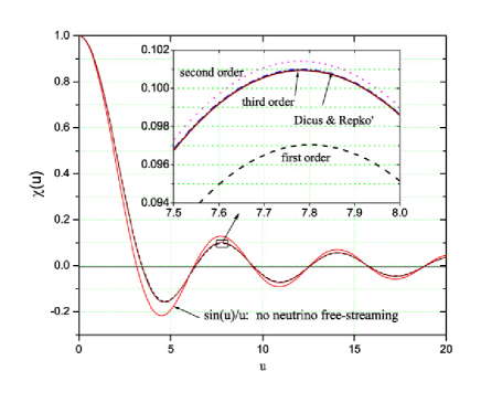
Figure 1: Under the approximations in Eq.(35), the solutions by our method are compared with that in Ref.[15].

Our calculation reveals that the neutrino damping on the RGWs is mainly pronouncing only in the frequency range $\nu\simeq(10^{-16}\sim 10^{-10})$ Hz, which corresponds to $k\simeq(10^{2}\sim 10^{8})$ and $\alpha\simeq(10^{-7}\sim 10^{-1})$. Outside this range the neutrino damping barely alters the RGWs. Figure 2 shows that our solution of short ($\nu\geq 10^{-10}$Hz) and long ($\nu\leq 10^{-16}$ Hz) modes almost overlap the homogeneous solution without neutrino free-streaming. For the short modes reentering the horizon well before the decoupling, the factor $1/u^{2}$ on the r.h.s. of Eq.(78) is very small and the inhomogeneous term is negligible. For those long modes, they are still outside the horizon during the neutrino free streaming, and are not affected by the damping. Only much later do these modes reenter the horizon, the neutrino density $f_{\nu}(u)$ becomes negligibly small, the homogeneous solution is valid for these long modes. Therefore, in long and short wavelength limit, the solution for RGWs is practically that of the homogeneous equation. Moreover, the upper panel of Figure 2 shows that, at the neutrino decoupling time $\eta_{dec}$, the time derivative of the short mode function $\chi^{\prime}(\eta_{dec})$ deviates from zero considerably. Therefore, the approximation in Eq.(35) is not accurate enough for the short modes of RGWs.

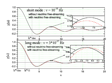
Figure 2: Neutrino free-streaming barely affects the short (upper) and the long modes (lower).

The matter-dominant stage has

$$h_{k}(\eta)=z^{-\frac{3}{2}}\Big{[}D_{1}J_{\frac{3}{2}}(k\,z)+D_{2}N_{\frac{3}{2}}(k\,z)\Big{]},\,\,\,\,\eta_{2}\leq\eta\leq\eta_{E}$$ (36)

where $z\equiv\eta-\eta_{m}$ and

$$D_{1}=\frac{-1}{2}\pi\,z_{2}^{\frac{5}{2}}\big{[}kN_{\frac{5}{2}}(k\,z_{2})h_{k}(\eta_{2})+N_{\frac{3}{2}}(k\,z_{2})h_{k}^{\prime}(\eta_{2})\big{]},$$ (37)

$$D_{2}=\frac{1}{2}\pi\,z_{2}^{\frac{5}{2}}\big{[}kJ_{\frac{5}{2}}(k\,z_{2})h_{k}(\eta_{2})+J_{\frac{3}{2}}(k\,z_{2})h_{k}^{\prime}(\eta_{2})\big{]},$$ (38)

withe $z_{2}\equiv\eta_{2}-\eta_{m}$. In the expressions of $D_{1}$ and $D_{2}$, the mode functions $h_{k}(\eta_{2})$ and $h^{\prime}_{k}(\eta_{2})$ are again from the precedent stage.

The accelerating stage has

$$h_{k}(\eta)=s^{\frac{1}{2}+\gamma}\Big{[}E_{1}J_{-\frac{1}{2}-\gamma}(k\,s)+E_{2}N_{-\frac{1}{2}-\gamma}(k\,s)\Big{]},\,\,\,\,\,\eta_{E}\leq\eta\leq\eta_{H}$$ (39)

where $s\equiv\eta-\eta_{a}$ and

$$E_{1}=\frac{-1}{2}\pi\,s_{E}^{\frac{1}{2}-\gamma}\big{[}kN_{\frac{1}{2}-\gamma}(k\,s_{E})h_{k}(\eta_{E})+N_{-\frac{1}{2}-\gamma}(k\,s_{E})h_{k}^{\prime}(\eta_{E})\big{]},$$ (40)

$$E_{2}=\frac{1}{2}\pi\,s_{E}^{\frac{1}{2}-\gamma}\big{[}kJ_{\frac{1}{2}-\gamma}(k\,s_{E})h_{k}(\eta_{E})+J_{-\frac{1}{2}-\gamma}(k\,s_{E})h_{k}^{\prime}(\eta_{E})\big{]},$$ (41)

with $s_{E}\equiv\eta_{E}-\eta_{a}$. So far, the explicit solution of $h_{k}(\eta)$ has been obtained for all the expansion stages, from Eq.(23) through Eq.(39).

The above detailed expressions of $h_{k}(\eta)$ are the major ingredients to determine the the spectrum of RGWs in the accelerating universe. What kind of RGWS would a matter-dominant universe have? To compare with the spatially flat accelerating universe, this non-accelerating universe is assumed to be also spatially flat with $\Omega_{m}+\Omega_{r}=1$. It should also go through the consecutive expansion stages listed previously, from the inflation to the matter-dominant, except the accelerating stage that is replaced by a continuation of the matter-dominant stage up to the present time $\eta_{H}$. In each stage the mode function $h_{k}(\eta)$ is of the same form as those given in Eqs.(23), (26), (29), (33), and (36), respectively. But the time duration of the matter stage for Eq.(36) is now extended to $\eta_{2}\leq\eta\leq\eta_{H}$. In both the accelerating and the matter-dominant models the mode $h_{k}(\eta)$ is sensitive to the scale factor $a(\eta)$ determined by their respective Friedmann equation (7), in which one sets $\rho_{\Lambda}=0$ for the matter-dominant model. To have a specific comparison of the two models, let us start at the time $\eta_{2}$ of the equality of radiation-matter with $1+z=3454$, when $\rho_{\Lambda}\ll\rho_{m}=\rho_{r}$, and it can be assumed that both models have the same initial values $a(\eta_{2})$ and $a^{\prime}(\eta_{2})$. Instead of the sudden transition approximation as in Eqs.(5) and (6), we solve numerically the Friedmann equation in both models up to the present time $\eta_{H}$ with $z=0$. Doing this is equivalent to assuming that both models would have an equal age of the universe. As a result, it is found that the scale factor $a(\eta_{H})$ in the accelerating model is $\sim 1.3$ times of that in the matter-dominant model shown in Fig.3.

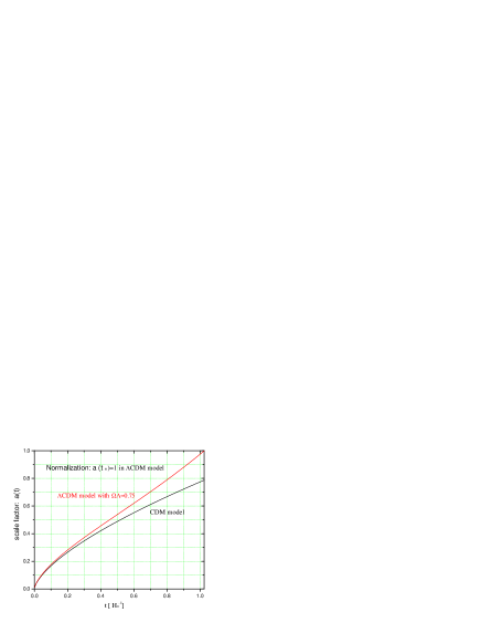
Figure 3: The scale factor $a(t)$ in the accelerating, and non-accelerating models, respectively.

This difference of $a(\eta_{H})$ will consequently cause a difference in the spectra for the two models. As is known [1, 3], inside the horizon the amplitude of modes $h_{k}(\eta)\propto 1/a(\eta)$, so the matter-dominant model would predict a spectral amplitude higher than the accelerating model. Indeed, our analytic calculation demonstrates that the ratio of the spectral amplitudes of CDM over those of $\Lambda$CDM is $\sim 1.3$. Moreover, we like to emphasize that there are some subtleties with the matter-dominant models, regarding to interpretation of the current cosmological observations. The actual universe is an accelerating one, so the observed Hubble constant is properly interpreted as the current expansion rate in the accelerating model, $H_{0}=a^{\prime}/a^{2}(\eta_{H})$. However, as our calculation has shown, the virtual matter-dominant universe would have a smaller rate $a^{\prime}/a^{2}(\eta_{H})\simeq 0.65\,H_{0}$. In this regard, Ref.[16] uses the observed Hubble constant $H_{0}$ as the current expansion rate of the virtual matter-dominant universe. This would give a spectrum with amplitude lower by an extra factor $\sim 1.3$ than it should have.

4. Spectrum of relic gravitational waves

The spectrum of RGWs $h(k,\eta)$ at a time $\eta$ is defined by the following equation [17]:

$$\int_{0}^{\infty}h^{2}(k,\eta)\frac{dk}{k}\equiv\langle 0|h^{ij}(\textbf{x},\eta)h_{ij}(\textbf{x},\eta)|0\rangle,$$ (42)

where the right-hand side is the expectation value of the $h^{ij}h_{ij}$. Calculation yields the spectrum, which is related to the mode function $h_{k}(\eta)$ as follows

$$h(k,\eta)=\frac{2}{\pi}k^{3/2}|h_{k}(\eta)|,$$ (43)

where the factor $2$ counts for the two independent polarizations. At present with time $\eta_{H}$ the spectrum is

$$h(k,\eta_{H})=\frac{2}{\pi}k^{3/2}|h_{k}(\eta_{H})|.$$ (44)

Note that this expression is formally different from the previous one in Refs.[3] only because here we use a different expansion for $h_{ij}(\eta,{\bf x})$ in Eq.(19). One of the most important properties of the inflation is that the initial spectrum of GRWs at the time $\eta_{i}$ of the horizon-crossing during the inflation is nearly scale-invariant [17]:

$$h(k,\eta_{i})=A(\frac{k}{k_{H}})^{2+\beta},$$ (45)

where $2+\beta\simeq 0$, and $A$ is a $k$-independent constant to be fixed by the observed CMB anisotropies in practice. The First Year WMAP gives the scalar spectral index $n_{s}=0.99\pm 0.04$ [9]. The Three Year WMAP gives $n_{s}=0.951^{+0.015}_{-0.019}$ [10], while in combination with constraints from SDSS, SNIa, and the galaxy clustering, it would give $n_{s}=0.965\pm 0.012$ (68% CL) [11]. From the relation $n_{s}=2\beta+5$ [1, 3], we have the inflation index $\beta=-2.02$ for $n_{s}=0.951$. Note that the constant $A$ is directly proportional to $A_{0}$ in Eq.(23) through the relation (43). Since the observed CMB anisotropies [9] is $\Delta T/T\simeq 0.37\times 10^{-5}$ at $l\sim 2$, which corresponds to anisotropies on scales of the Hubble radius $1/H_{0}$, so, as in Refs.[3], we take the normalization of the spectrum

$$h(k_{E},\eta_{H})=0.37\times 10^{-5}r^{\frac{1}{2}},$$ (46)

where $k_{E}=\frac{k_{H}}{(1+z_{E})}=\frac{2\pi\gamma}{(1+z_{E})}$ is the wave number that crosses the horizon at $\eta_{E}$, its corresponding physical frequency being $\nu_{E}=k_{E}/2\pi a(\eta_{H})=H_{0}/(1+z_{E})\sim 1\times 10^{-18}$ Hz, $r$ is taken as a parameter roughly representing the tensor/scalar ratio. In Eq.(46) it is $r^{\frac{1}{2}}$ rather than $r$ as in Ref.[3]. The value of the ratio $r$ is an important issue and is still unsettled yet. However, as examined in details in Ref.[20], the relative contributions from the RGWs and from the density perturbations are, in fact, frequency-dependent; thus, generally speaking, for different frequency ranges $r$ can take on a different values. Therefore, in our treatment, for simplicity, $r$ is only taken as a constant parameter for normalization of RGWs, and does not accurately represent the actual relative contributions. Currently, only observational constraints on $r$ have been given. Recently the Three Year WMAP constraint is $r<2.2$ ($95\%$ CL) evaluated at $k=0.002$ Mpc^-1, and the full WMAP constraint is $r<0.55$ (95% CL) [12]. The combination from such observations, as of the Lyman-$\alpha$ forest power spectrum from SDSS, 3-year WMAP, supernovae SN, and galaxy clustering, gives an upper limit $r<0.22$ ($95\%$ CL) [11]. Moreover, the ratio $r$ may be allowed to take on different values on different range of frequency, but we will take a constant $r$ for simplicity.

The spectral energy density $\Omega_{g}(k)$ of the RGWs is given by

$$\Omega_{g}(k)=\frac{\pi^{2}}{3}h^{2}(k,\eta_{H})\Big{(}\frac{k}{k_{H}}\Big{)}^{2},$$ (47)

directly associated with the spectrum of RGWs $h(k,\eta_{H})$ in Eq.(44). This follows from the definition [17, 20]

$$\Omega_{GW}\equiv\frac{\rho_{g}}{\rho_{c}}=\int_{k_{low}}^{k_{upper}}\Omega_{g}(k)\frac{dk}{k},$$ (48)

where $\rho_{g}=\frac{1}{32\pi G}h_{ij,0}h^{ij}_{,0}$ is the energy density of RGWs, and $\rho_{c}=3H_{0}^{2}/8\pi G$ is the critical energy density. The integration in Eq.(48) has the lower and upper limits, $k_{low}$ and $k_{upper}$, as the cutoffs of the wavenumber. For the lower limit $k_{low}$, the corresponding wavelength may be taken to be the current Hubble radius, $\lambda_{low}=1/H_{0}$. This is because the waves with wavelengths longer than $1/H_{0}$ should be treated as part of the space-time background and should not be included to the energy of RGWS [1] [21]. By Eq.(15), the corresponding frequency

$$\nu_{low}\simeq 2\times 10^{-18}{\,\rm Hz}.$$ (49)

The upper limit $k_{upper}$ can be determined by as the following. During the inflation the modes of GRWs with wavenumbers greater than the expansion rate $H(\eta_{i})$ are approaching the adiabatic limit, therefore, their generation is thus effectively suppressed [19]. Taking the scale of the vacuum energy driving the inflation to be $E_{vac}\sim 10^{16}$ Gev, typical of Grand Unified Theories, then $H(\eta_{i})\sim 10^{13}$ Gev $\simeq 10^{38}$ Hz. During the subsequent stages of cosmic expansion, the corresponding frequency $\nu$ of this value will be redshifted by a factor $a(\eta_{i})/a(\eta_{H})\sim 10^{-29}$; thus one has

$$\nu_{upper}\simeq 10^{10}{\,\rm Hz}.$$ (50)

If the energy scale for the inflation is lower than $10^{16}$ Gev, then the upper limit $\nu_{upper}$ will be lower than that in Eq.(50) correspondingly. These lower and upper integration limits in Eqs.(49) and (50) also ensure the convergence of the integration of Eq.(48).

In the absence of direct detection of RGWs, the constraints on the energy density $\Omega_{GW}$ is more relevant. Given the model parameters $\beta$, $\beta_{s}$, $\gamma$, and $r$, the definite integration of Eq.(48) yields $\Omega_{GW}$ of RGWs. For the fixed parameters $r=0.22$, $\Omega_{\Lambda}=0.75$, and $\beta_{s}=-0.3$, one finds $\Omega_{GW}=1.12\times 10^{-2}$ for the inflationary model of $\beta=-1.8$. Such a large energy density will inevitably affect the expansion rate of the universe at a temperature $T\sim$ a few MeV when the nucleosynthesis process is going on. The nucleosythesis bound is [22]

$$\Omega_{GW}h^{2}<8.9\times 10^{-6}$$ (51)

with $h\sim 0.71$ being the Hubble parameter [9]. Thus the $\beta=-1.8$ model with $r=0.22$ predicts an energy density $\Omega_{GW}$ being some four orders higher than the upper bound given Eq.(51). So this model will be in jeopardy, unless the parameter $r$ is much smaller than $0.22$. Under the same set of parameters $r=0.22$, $\Omega_{\Lambda}=0.75$, and $\beta_{s}=-0.3$, the model of $\beta=-1.9$ gives $\Omega_{GW}=2.04\times 10^{-8}$, and the model of $\beta=-2.02$ gives $\Omega_{GW}=1.54\times 10^{-14}$, both models are safely below the nucleosythesis bound in Eq.(51).

In the following we demonstrate the details of the resulting spectra $h(k,\eta_{H})$ and $\Omega_{g}(k)$ of RGWs, their explicit dependence upon the model parameters $\beta$, $\beta_{s}$, $\gamma$, and the modifications by the neutrino damping.

Figure 4 gives the spectrum $h(\nu,\eta_{H})$ as a function of the frequency $\nu$ without neutrino free streaming. To show the dependence upon the inflationary models, for the fixed $r=0.22$, $\Omega_{\Lambda}=0.75$, $\beta_{s}=-0.3$, we plot $h(\nu,\eta_{H})$ in three models of $\beta=-1.8$, $-1.9$, and $-2.02$. It is seen that $h(\nu,\eta_{H})$ is very sensitive to $\beta$. A smaller $\beta$ will generate less power of RGWs for all frequencies. The details of the spectrum is similar to that given in Refs.[3].

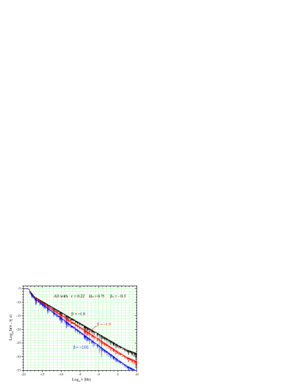
Figure 4: The spectrum $h(\nu,\eta_{H})$ of GRW is very sensitive to the inflation parameter $\beta$.

Figure 5 gives the comparison of the sensitivity curve of the ground-based interferometer LIGO with the spectra of $\beta=-1.8$, $-1.9$, and $-2.02$ from Fig.4. Here the vertical axis is the root mean square amplitude per root Hz, which equals to

$$\frac{h(\nu)}{\sqrt{\nu}}.$$ (52)

Note that, relevant to LIGO, the frequency range is $(10\sim 10^{4})$ Hz, which is not to be affected by the neutrino damping. Obviously from the plot, the LIGO I SRD [4] is yet not able to detect the signals of RGWs in the $\beta=-1.8$ model even with a very large ratio $r=2.2$. Therefore, LIGO is unlikely to able detect the RGWs, as it currently stands. The Advanced LIGO with greatly enhanced sensitivity [4] will be able to put a tighter constraints on the parameters.

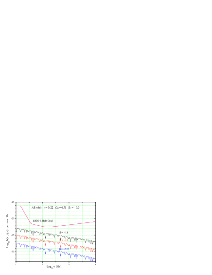
Figure 5: Comparison of the spectra with the LIGO I SRD Goal sensitivity curve that has already been achieved by S5 of LIGO [4]. The vertical axis is the r.m.s amplitude per root Hz defined in Eq.(52).

Figure 6 is a comparison of the LISA sensitivity curve with the spectra from Fig.4 in the frequency range $(10^{-7},10^{0})$ Hz. Although these frequencies are lower than that for LIGO, it is still not to be affected by the neutrino damping either. Assuming that LISA has one year observation time, which corresponds to frequency bin $\Delta\nu=3\times 10^{-18}$Hz (i.e., one cycle/year) around each frequency. Thus, to make a comparison with the sensitity curve, we need to rescale the spectrum $h(\nu)$ in Eq.(44) into the root mean square spectrum $h(\nu,\Delta\nu)$ in the band $\Delta\nu$ [17],

$$h(\nu,\Delta\nu)=h(\nu)\sqrt{\frac{\Delta\nu}{\nu}}.$$ (53)

This r.m.s spectrum can be directly compared with the 1 year integration sensitivity curve that is downloaded from LISA [23]. The plot shows that LISA by its present design will be able to easily detect the RGWs in the inflationary model of $\beta=-1.8$. If the ratio $r>0.22$, LISA will also be able to detect the inflationary models of $\beta=-1.9$. However, LISA is unlikely to be able to detect the model of $\beta=-2.02$. Here Fig. 5 and Fig. 6 also correct the mistake of Ref.[3], where improper comparison is made with the LIGO data and the LISA sensitive curve. As will be seen in the following, the neutrino free streaming practically affects only the spectrum in a frequency range of $(10^{-16}\sim 10^{-10})$, therefore, Fig. 5 and Fig. 6 are not to be changed by neutrinos.

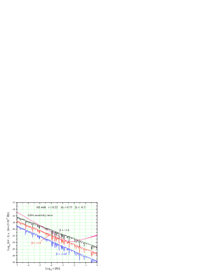
Figure 6: Comparison of the spectra with the LISA sensitivity curve [23]. The vertical axis is the r.m.s spectrum defined in Eq.(53). LISA will be able to detect the inflationary models of $\beta=-1.8$ and $-1.9$.

The influence of reheating stage on the spectrum is shown in Fig.7. The spectra for three different values of $\beta_{s}=0.5$, $0$, $-0.3$ are given. It is clear that whereas the spectrum is almost unchanged by $\beta_{s}$ in the large portion of frequency range $\nu\leq 10^{7}$ Hz, a larger $\beta_{s}$ will damp the amplitude in a high frequency range $10^{7}\sim 10^{9}$Hz. However, around $\nu\sim 10^{9}$Hz the spectrum begins to increase considerably. This feature of RGWs in the GHz range is very interesting, as this high-frequency range of RGWs is the scientific gaol of some electromagnetic detecting systems, such as the one using a Gaussian laser beam [24], or a circulating microwave beam [25]. However, the predicted spectrum for the very high frequency range $\nu>10^{10}$ Hz is not reliable, since the energy scale of the conventional inflationary models are less than $10^{16}$ Gev.

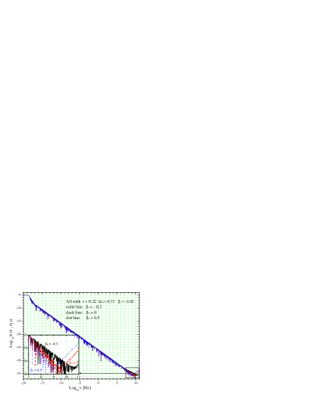
Figure 7: The reheating affects the spectrum $h(\nu,\eta_{H})$ only in very high frequency range $\nu>10^{7}$ Hz.

The influence of the dark energy on the spectrum $h(\nu,\eta_{H})$ is demonstrated in Fig.8, where $\Omega_{\Lambda}=0.0$, $0.7$, and $0.75$ are taken respectively. Over the whole range of frequency $10^{-19}\sim 10^{10}$ Hz, the amplitude of spectrum is altered by the presence of $\Omega_{\Lambda}$, but the slope remains the same. In regards to the amplitude, firstly, the spectrum in a matter-dominant universe of $\Omega_{\Lambda}=0$ is higher than those in an accelerating universe with $\Omega_{\Lambda}>0$, as Fig. 8 shows, roughly by a factor $\sim 1.3$. This feature is due to the fact the scale factor $a(t_{H})$ in the accelerating model is greater than that in the matter-dominant models, as has been explained at the ending paragraph of section 3. Secondly, among the accelerating models, by an analysis of the expression of $h(\nu,\eta_{H})$, the amplitude of $h(\nu,\eta_{H})$ is proportional to $(\frac{a(\eta_{E})}{a(\eta_{H})})^{3}=1/(1+z_{E})^{3}$, as has been explicitly shown in Ref.[3]. This phenomenon occurs basically because, starting from the time $\eta_{E}$ up to the present time $\eta_{H}$, the scale factor $a(\eta)$ increases by a different amount in models of different $\Omega_{\Lambda}$ ; thus, stretching of the physical wavelengths and damping of the mode $h_{k}(\eta)$ are different correspondingly. In the accelerating models with $\rho_{\Lambda}$ being constant, one has approximately $(\frac{a(\eta_{E})}{a(\eta_{H})})^{3}\simeq\Omega_{m}/\Omega_{\Lambda}$; thus, the amplitude of $h(\nu,\eta_{H})\propto\Omega_{m}/\Omega_{\Lambda}$, i.e., the model with more dark energy component has relatively a lower amplitude of $h(\nu,\eta_{H})$. Note that, in interpreting this relation $h(\nu,\eta_{H})\propto\Omega_{m}/\Omega_{\Lambda}$, the dark energy $\Omega_{\Lambda}$ should be large enough, say, $\Omega_{\Lambda}>\Omega_{m}$, to ensure the sufficiently accelerating expansion. This phenomenon is verified now in Fig.8, for example, the amplitude of the $\Omega_{\Lambda}=0.75$ model over that of the $\Omega_{\Lambda}=0.7$ is found to be $(\frac{0.25}{0.75})/(\frac{0.3}{0.7})\approx 0.8$.

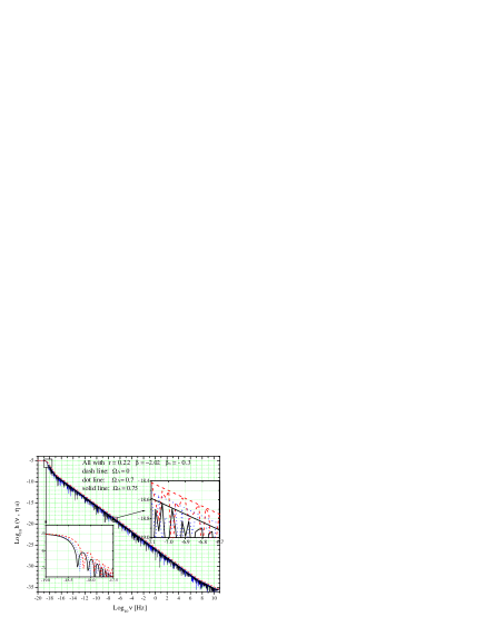
Figure 8: The dependence of $h(\nu,\eta_{H})$ upon the dark energy $\Omega_{\Lambda}$ in the accelerating universe.

Presented in Fig.9 is the modification of the spectrum $h(\nu,\eta_{H})$ by the neutrino free-streaming up to the first order approximation to Eq.(34). The effect is pronounced in the low frequency range $(10^{-16}\sim 10^{-10})$ Hz, where the amplitude of $h(\nu,\eta_{H})$ is reduced by a factor $\sim 20\%$ in comparison with the model without neutrino free streaming. Our analytical spectrum qualitatively agrees with the numerical result in Ref.[16] in the relevant range. As we have mentioned earlier, LIGO and LISA operating around $\sim 10^{2}$ Hz and $\sim 10^{-3}$ Hz, respectively, will not be able detect this neutrino damping. But CMB anisotropies and polarization may be affected by that.

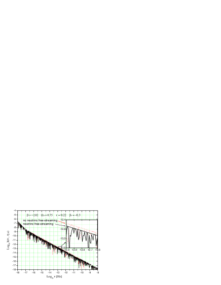
Figure 9: The neutrino free-streaming reduces $h(\nu,\eta_{H})$ in the frequency range $10^{-17}\sim 10^{-10}$ Hz.

The dependence of spectral energy density $\Omega_{g}$ in Eq.(47) on the inflationary models is illustrated in Fig.10. For the purpose of clarity, the neutrino free streaming is not taken into account. Clearly, $\Omega_{g}$ is very sensitive to the parameter $\beta$, and a larger $\beta$ gives a higher $\Omega_{g}$. The model of $\beta=-1.8$ has an $\Omega_{g}$ too high, and as mentioned in paragraph before Eq.(51), it has already been ruled out by the nucleosynthesis bound of Eq.(51). The Advanced LIGO [4] will be able to detect RGWs with $\Omega_{g}h^{2}>10^{-9}$ at $\nu\sim 100$Hz, and it might impose stronger constraints on other inflationary models.

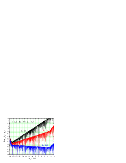
Figure 10: The spectral energy density $\Omega_{g}(\nu)$ for various inflation parameter $\beta$.

The impact of dark energy $\Omega_{\Lambda}$ on the spectral energy density $\Omega_{g}$ is plotted in Fig.11 for the model $\beta=-2.02$. It is clear seen that the accelerating expansion of the universe will cause a decrease of the amplitude of $\Omega_{g}$ over the whole range of frequencies, and a larger $\Omega_{\Lambda}$ gives a lower $\Omega_{g}$. Obviously, the effect due to the acceleration of expansion of the universe cannot be simply ignored.

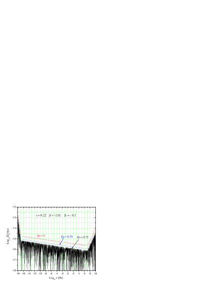
Figure 11: The spectral energy density $\Omega_{g}(\nu)$ for different $\Omega_{\Lambda}$. A larger $\Omega_{\Lambda}$ yields a lower $\Omega_{g}(\nu)$.

The damping effect of neutrino free-streaming on the spectral energy density $\Omega_{g}(\nu)$ is illustrated in Fig.12 for the model $\beta=-2.02$. The effect is mostly within the frequency range $10^{-16}\sim 10^{-10}$Hz, where the amplitude of $\Omega_{g}(\nu)$ drops visibly by a factor of $\sim 36\%$. Correspondingly, the energy density of RGWs in Eq.(48) is now reduces to $\Omega_{GW}=1.1\times 10^{-14}$ after considering the neutrino free-streaming. Recall that it was $\Omega_{GW}=1.54\times 10^{-14}$ without neutrino damping, thus the neutrino damping has caused a drop of $\sim 29\%$ of $\Omega_{GW}$. Our result is also qualitatively consistent with the numerical calculation in Ref. [16].

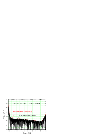
Figure 12: The neutrino free streaming reduces $\Omega_{g}(\nu)$ in the range $10^{-17}\sim 10^{-10}$Hz.

ACKNOWLEDGMENT: Y. Zhang’s work has been supported by the CNSF No.10173008, NKBRSF G19990754, SRFDP, and CAS. We thank Dr.L.Q. Wen at MPI for very helpful discussions.

In this appendix we derive the anisotropic stress tensor $\pi_{ij}$ of cosmic neutrinos during their free streaming, filling in the details skipped in Ref.[14]. Next we present the perturbation method to systematically solve the equation of GRWs. As a merit, this method applies for the realistic situation of a time-dependent fractional energy density $f_{\nu}(\eta)$ of neutrinos, a nonzero decoupling time $u_{dec}\neq 0$, and a non-vanishing time derivative $\chi^{\prime}(u_{dec})\neq 0$. This solution is an extension to the previous works in Refs.[14] [15]. The same notations as in Ref.[14] is used.

In the radiation stage at temperatures $\geq 2$ Mev , the neutrinos are in equilibrium with other relativistic species, such as electron and photons, together forming the radiation component. During this period, practically all the $k$-modes $h_{k}(\eta)$ of cosmological interest are still far outside the horizon, thus remain a constant, $h_{k}(\eta)\simeq$ constant, thus, are not effected by the neutrinos. With the further expansion of the universe when the temperature drops down to $<2$ Mev, the neutrinos are going out of equilibrium and are starting to stream freely in space. Then the neutrinos will be able to influence the modes $h_{k}(\eta)$ of short wavelengths that re-enter the horizon. The equation of RGWs then becomes inhomogeneous

$$h_{ij}^{\prime\prime}(\eta)+2\frac{a^{\prime}(\eta)}{a(\eta)}h_{ij}^{\prime}(\eta)-\nabla^{2}h_{ij}(\eta)=16\pi Ga^{2}\pi_{ij}(\eta).$$ (54)

Here the source term $\pi_{ij}$, contributed by neutrinos, is the anisotropic part of the stress tensor $T_{ij}$ and is effective only during the period $\eta_{dec}\leq\eta\leq\eta_{2}$, from the neutrinos decoupling up to the beginning of the matter domination. When the matter domination begins, the neutrino number density has been diluted out by a factor $\sim 10^{-3\times 6}$, so the source $\pi_{ij}$ is effectively switched off after the matter domination. In terms of the neutrino distribution function $n({\bf x,p},t)$ and the momentum $p^{i}$, the spatial part of the neutrino energy-momentum stress tensor is written as

$$T^{i}_{\,\,j}=\frac{1}{\sqrt{-g}}\int d^{3}{\bf p}\,n({\bf x,p},t)p^{i}p_{j}/p^{0}.$$ (55)

To keep the same notation with Ref.[14], here the cosmic time $t=\int a(\eta)d\eta$ is used. In the presence of the perturbations $h_{ij}$ of the metric, $n({\bf x,p},t)$, $p^{i}$, and $p^{0}$ all depends on $h_{ij}$. So the stress tensor is written as a sum of

$$T^{i}_{j}=P\delta_{ij}+\pi_{ij},\,\,\,\,\,{i,j=1,2,3}$$ (56)

where $P\delta_{ij}$ is the unperturbed part with $P$ being the homogeneous and isotropic pressure, and the anisotropic stress tensor $\pi_{ij}$ is the perturbed part caused by $h_{ij}$

$$\pi_{ij}({\bf x},t)=\frac{1}{\sqrt{-g}}\,\delta\int d^{3}{\bf p}\,n({\bf x,p},t)\frac{p^{i}p_{j}}{p^{0}}.$$ (57)

Since $h_{ij}$ is small, only the first order of $h_{ij}$ is needed in evaluating $\pi_{ij}$. The distribution function $n({\bf x,p},t)$ satisfies the Boltzmann equation

$$\frac{\partial n}{\partial t}+\frac{\partial n}{\partial x^{i}}\frac{dx^{i}}{dt}+\frac{\partial n}{\partial p_{i}}\frac{dp_{i}}{dt}=0.$$ (58)

With $dx^{i}/dt=p^{i}/p^{0}$ and the geodesic equation $dp_{i}/dt=\frac{1}{2}g_{\gamma\delta,i}p^{\gamma}p^{\delta}=\frac{1}{2}h_{jk,i}p^{j}p^{k}$, Eq.(58) can be expanded as

$$\frac{\partial n}{\partial t}+\frac{p^{i}}{p^{0}}\frac{\partial n}{\partial x^{i}}+\frac{1}{2}h_{jk,i}\frac{p^{j}p^{k}}{p^{0}}\frac{\partial n}{\partial p_{i}}=0.$$ (59)

At the instant $t_{dec}$ of the decoupling the neutrinos are still an ideal gas, so one writes

$$n({\bf x,p},t)=n({\bf x,p},t_{dec})+\delta n({\bf x,p},t),$$ (60)

where

$$n({\bf x,p},t_{dec})=\frac{N}{(2\pi)^{3}}\Big{[}\exp\Big{(}\sqrt{g^{ij}(\textbf{x},t_{dec})p_{i}p_{j}}/T_{dec}\Big{)}+1\Big{]}^{-1}$$ (61)

is the distribution function of the ideal gas of temperature $T_{dec}$, and $\delta n$ represents the perturbation satisfying $\delta n=0$ at $t_{dec}$. In our treatment $p_{i}$ is treated as the unperturbed momentum and $p^{i}=g^{ij}p_{j}$ as the perturbed one. Substituting Eq.(60) into Eq.(59), neglecting the higher order term $\frac{1}{2}h_{jk,i}\frac{p^{j}p^{k}}{p^{0}}\frac{\partial\delta n}{\partial p_{i}}$, using $\partial n_{dec}/\partial t=0$,

$$\frac{\partial n_{dec}}{\partial x^{i}}=-\frac{1}{2}\bar{n}^{\prime}(p)\,p\hat{p_{j}}\hat{p_{k}}\frac{\partial}{\partial x^{i}}h_{jk}({\bf x},t_{dec}),$$ (62)

(Ref.[14] missed a factor $\frac{1}{2}$ in Eq.(62)), and $\partial n/\partial p_{i}=\bar{n}^{\prime}(p)\hat{p_{i}}$, where $\bar{n}^{\prime}(p)\equiv\partial\bar{n}/\partial p$, $\hat{p_{i}}\equiv p_{i}/p$ and $p\equiv\sqrt{p_{i}p_{i}}$, the Boltzmann equation reduces to the following

$$\frac{\partial\delta n}{\partial t}+\frac{\hat{p_{i}}}{a(t)}\frac{\partial\delta n}{\partial x^{i}}=-\frac{p}{2a(t)}\bar{n}^{\prime}(p)\hat{p_{i}}\hat{p_{j}}\hat{p_{k}}\frac{\partial}{\partial x^{k}}(h_{ij}({\bf x},t)-h_{ij}({\bf x},t_{dec})),$$ (63)

where $\bar{n}(p)=\frac{N}{(2\pi)^{3}}[\exp(p/T_{dec}a_{dec})+1]^{-1}$. This equation can be decomposed into the Fourier $\bf k$-modes, as in Eq.(19), and each mode has the formal solution

$$\delta n_{k}({\bf p},\eta)=-\frac{i}{2}p\bar{n}^{\prime}(p)\hat{p_{i}}\hat{p_{j}}\hat{p}\cdot{\bf k}\int^{\eta}_{\eta_{dec}}d\eta^{\prime}e^{i\hat{p}\cdot{\bf k}(\eta^{\prime}-\eta)}\Big{[}h_{ij}(k,\eta^{\prime})-h_{ij}(k,\eta_{dec})\Big{]},$$ (64)

where the comoving time $d\eta=dt/a$ is used, and the integrand function depends on $h_{ij}$ explicitly, where

$$h_{ij}(k,\eta)\equiv\sum_{\sigma}\epsilon^{\sigma}_{ij}h_{k}^{(\sigma)}(\eta).$$ (65)

Defining the variable $u\equiv k(\eta-\eta_{dec})$, Eq.(64) just reduces to Eq.(13) in Ref.[14]. There are four terms that contribute to $\pi_{ij}$ in Eq.(57). Specifically, the perturbations to the distribution function $n$ give two terms:

$$\frac{p^{i}p_{j}}{p^{0}}\delta n_{k}(\eta_{dec})=-\frac{p^{2}}{2a}\bar{n}^{\prime}(p)\hat{p_{i}}\hat{p_{j}}\hat{p_{m}}\hat{p_{l}}h_{ml}(k,\eta_{dec}),$$ (66)

$$\frac{p^{i}p_{j}}{p^{0}}\delta n_{k}(\eta)=-\frac{p^{2}}{2a}\bar{n}^{\prime}(p)\hat{p_{i}}\hat{p_{j}}\hat{p_{m}}\hat{p_{l}}\Big{[}h_{ml}(k,\eta)-h_{ml}(k,\eta_{dec})-\int^{\eta}_{\eta_{dec}}d\eta^{\prime}e^{i\hat{p}\cdot\vec{k}(\eta^{\prime}-\eta)}h^{\prime}_{ml}(k,\eta^{\prime})\Big{]},$$ (67)

where integration by parts with respect to the time $\eta^{\prime}$ has been used, the following two terms also contribute

$$\frac{\bar{n}(p)}{p^{0}}p_{j}\delta p^{i}=-\frac{p}{a}\bar{n}\hat{p_{l}}\hat{p_{j}}h_{il}(k,\eta),$$ (68)

$$-\frac{\bar{n}p^{i}p_{j}}{(p^{0})^{2}}\delta p^{0}=\frac{p}{2a}\bar{n}\hat{p_{i}}\hat{p_{j}}\hat{p_{m}}\hat{p_{l}}h_{ml}(k,\eta).$$ (69)

One puts these four terms from Eq.(66) through Eq.(69) into Eq.(57) and carries out the integration $\int d^{3}{\bf p}$. The spherical coordinates with $z=\bf\hat{k}$ can be used in doing the angular integration, so that $\hat{p}\cdot\bf\hat{k}=\cos\theta\equiv\mu$. Since $h_{ml}$ is transverse, one has

$$\int d\Omega\,\hat{p_{i}}\hat{p_{j}}\hat{p_{m}}\hat{p_{l}}h_{ml}=\frac{\pi}{4}(\delta_{im}\delta_{jl}+\delta_{il}\delta_{jm})h_{ml}\int^{1}_{-1}d\mu(1-\mu^{2})^{2}.$$ (70)

After some calculation, one arrives at the resulting anisotropic stress

$$\pi_{ij}=-4\bar{\rho}_{\nu}(\eta)\int_{\eta_{dec}}^{\eta}d\eta^{\prime}K(k\eta-k\eta^{\prime})h^{\prime}_{ij}(\eta^{\prime}),$$ (71)

where $\bar{\rho}_{\nu}(\eta)=a^{-4}\int d^{3}p\,p\bar{n}(p)$ is the neutrino density, and $K$ is the kernel defined as

$$K(s)=\frac{1}{16}\int_{-1}^{1}d\mu\,(1-\mu^{2})^{2}e^{i\mu s}=\frac{j_{2}(s)}{s^{2}},$$ (72)

with $j_{2}(s)$ is the spherical Bessel function. Since $h_{ij}$ is traceless and transverse, so is $\pi_{ij}$, by Eq.(71), with $\pi^{i}_{\,\,i}=0$ and $\pi_{ij,j}=0$. Substituting Eq.(71) into Eq.(54) and using the Friedmann equation $a^{\prime}\,{}^{2}/a^{4}=8\pi G\bar{\rho}/3$ yields the integro-differential equation [14]

$$h_{k}^{\prime\prime}(\eta)+\frac{2a^{\prime}(\eta)}{a(\eta)}h_{k}^{\prime}(\eta)+k^{2}h_{k}(\eta)=-24f_{\nu}(\eta)\Big{[}\frac{a^{\prime}(\eta)}{a(\eta)}\Big{]}^{2}\int_{\eta_{dec}}^{\eta}d\eta^{\prime}K(k\eta-k\eta^{\prime})h_{k}^{\prime}(\eta^{\prime}),$$ (73)

where the fractional neutrino energy density

$$f_{\nu}(\eta)\equiv\frac{\bar{\rho}_{\nu}(\eta)}{\bar{\rho}(\eta)}.$$ (74)

Although at present the dark energy $\Omega_{\Lambda}$ is dominant, but it is negligible during the radiation-dominant stage, in comparison with the matter, neutrino, and radiation components. Even in the dynamic models of dark energy evolving with time, the contribution from $\rho_{\Lambda}(\eta)$ during radiation-dominant stage is not allowed to be more than a few percent of the total energy [26] [27]. Therefore, Eq.(74) is practically equal to

$$f_{\nu}(\eta)=\frac{f_{\nu}(0)}{1+a(\eta)/a_{eq}}\,,$$ (75)

where $a_{eq}=a(\eta_{2})$ is the scale factor at the radiation-matter equality, and

$$f_{\nu}(0)=\frac{\Omega_{\nu}}{\Omega_{\nu}+\Omega_{\gamma}},$$ (76)

with $\Omega_{\nu}$ and $\Omega_{\gamma}$ being the present fractional energy density o f the neutrinos and the radiation, respectively. Since $\eta_{dec}\gg\eta_{e}$, we can write $a(\eta)=a_{e}\eta$ with $a_{e}$ defined in Eq.(4) for the radiation-dominant stage. Introducing the variable $u\equiv k\eta$ and setting

$$h_{k}(u)=h_{k}(\eta_{dec})\chi(u),$$ (77)

then Eq.(73) is reduced to

$$\chi^{\prime\prime}(u)+\frac{2}{u}\chi^{\prime}(u)+\chi(u)=-24\frac{f_{\nu}(0)}{u^{2}(1+\alpha\,u)}\int_{u_{dec}}^{u}dUK(u-U)\chi^{\prime}(U),$$ (78)

where $\alpha\equiv a_{e}/k\,a_{eq}$.

Dicus & Repko [15] present an analytical solution of Eq.(78) under the approximation of setting $u_{dec}=0$, $\alpha=0$ and $\chi^{\prime}(\eta_{dec})=0$. This is only valid for those modes that reenter the horizon well after the neutrino decoupling. Note that, in the coordinate that is used, the decoupling time $u_{dec}\neq 0$ as in Eq.(Analytic spectrum of relic gravitational waves modified by neutrino free streaming and dark energy). Besides, for the short wavelength modes the derivative $\chi^{\prime}(\eta_{dec})\neq 0$. Moreover, actually $\alpha u=1$ at the time $\eta_{2}$, thus, setting $\alpha=0$ for the whole period $(\eta_{dec},\eta_{2})$ would lead to an over-account of the fractional neutrino energy density $f_{\nu}(\eta)$ and consequently would give a lower amplitude of RGWs. Unlike in Refs.[14, 15] , here we do not make the above-mentioned approximation, but instead, keep $u_{dec}$, $\alpha$ and $\chi^{\prime}(\eta_{dec})$ as they are. We use a perturbation method to solve the integro-differential equation (78) analytically, which can achieve high accuracy as one requires. Note that the source term on the r.h.s. of Eq.(78) is relatively small, and setting it to be zero yields the homogeneous equation

$$\chi_{0}^{\prime\prime}(u)+\frac{2}{u}\chi_{0}^{\prime}(u)+\chi_{0}(u)=0,$$ (79)

with the solution

$$\chi_{0}(u)=c_{1}\frac{e^{iu}}{u}+c_{2}\frac{e^{-iu}}{u},$$ (80)

as the $0$^th order approximation to Eq.(78), where $c_{1}$ and $c_{2}$ are the coefficients determined by the continuity condition at $u_{dec}$. One substitutes $\chi^{\prime}_{0}(u)$ in place of $\chi^{\prime}(u)$ in the integration of Eq.(78) to give the $1^{st}$ order approximation

$$\chi_{1}^{\prime\prime}(u)+\frac{2}{u}\chi_{1}^{\prime}(u)+\chi_{1}(u)=-24\frac{f_{\nu}(0)}{u^{2}(1+\alpha\,u)}\int_{u_{dec}}^{u}dUK(u-U)\chi_{0}^{\prime}(U),$$ (81)

which is a differential equation with a known inhomogeneous term. It has a particular solution

$$\chi^{*}(u) = \int^{u}_{u_{dec}}\frac{y_{2}(u)y_{1}(v)-y_{1}(u)y_{2}(v)}{W[y_{1},y_{2}](v)}r(v)dv$$ (82)

$$= -\frac{24f_{\nu}(0)}{u}\int^{u}_{u_{dec}}dv\frac{\sin(u-v)}{v(1+\alpha v)}\int^{v}_{u_{dec}}ds\frac{j_{2}(v-s)}{(v-s)^{2}}\chi_{0}^{\prime}(s),$$

where $r(v)$ represents the inhomogeneous term of Eq.(81), and $y_{1}=\frac{e^{iu}}{u}$, $y_{2}=\frac{e^{-iu}}{u}$ are the two linearly independent solutions to the homogeneous counterpart, and $W[y_{1},y_{2}](v)=-2i/v^{2}$ is the Wronskian. Therefore, the solution of Eq.(81) is given by

$$\chi_{1}(u)=\chi_{0}(u)+\chi^{*}(u),$$ (83)

which is also the $1^{st}$ order approximate solution of Eq.(78). Similarly, one substitutes the $1^{st}$ order solution $\chi_{1}(u)$ into Eq.(82), and obtains the $2^{nd}$ order approximate equation,

$$\chi_{2}^{\prime\prime}(u)+\frac{2}{u}\chi_{2}^{\prime}(u)+\chi_{2}(u)=-24\frac{f_{\nu}(0)}{u^{2}(1+\alpha\,u)}\int_{u_{dec}}^{u}dUK(u-U)\chi_{1}^{\prime}(U),$$ (84)

which has a particular solution

$$\chi^{**}(u)=-\frac{24f_{\nu}(\eta_{dec})}{u}\int^{u}_{u_{dec}}dv\frac{\sin(u-v)}{v(1+\alpha v)}\int^{v}_{u_{dec}}ds\frac{j_{2}(v-s)}{(v-s)^{2}}\chi_{1}^{\prime}(s),$$ (85)

and thus the $2^{nd}$ order approximate solution is

$$\chi_{2}(u)=\chi_{0}(u)+\chi^{**}(u).$$ (86)

By the same routine, the higher order solutions can be obtained. In fact, as our calculation shows that the $1^{st}$ order approximation is already accurate enough for the purpose of computing the spectrum for RGWs. An important advantage of our solution is that it is valid for those modes that reenter the horizon before or after the decoupling time $\eta_{dec}$. Integrations, such as in Eqs.(82) and (85), can be done easily by common computing tools.

References

[*]e-mail: yzh@ustc.edu.cn
[1] L. P. Grishchuk,
Sov.Phys.JETP 40, 409 (1975);
Class.Quant.Grav.14, 1445 (1997);
astro-ph/0008481.
[2] A. A. Starobinsky,
JEPT Lett. 30 682 (1979);
Sov.Astron.Lett.11, 133 (1985);
V. A. Rubakov, M.Sazhin, and A. Veryaskin,
Phys.Lett.B 115, 189 (1982);
R. Fabbri & M.D. Pollock,
Phys.Lett.B125, 445 (1983);
L. F. Abbott & M.B. Wise,
Nucl.Phys.B244, 541 (1984);
L. F. Abbott & D. D. Harari, Nucl.Phys.B264, 487(1986);
B. Allen, Phys.Rev.D37, 2078 (1988);
V. Sahni, Phys.Rev.D42, 453 (1990);
A. Riszuelo & J. P. Uzan,
Phys.Rev.D62, 083506 (2000);
H. Tashiro, et.al,
Class.Quant.Grav.21, 1761 (2004);
A. B. Henriques,
Class.Quant.Grav.21, 3057 (2004);
W.Zhao and Y.Zhang,
Phys.Rev.D74, 043503 (2006).