General relativistic simulations of passive-magneto-rotational
core collapse with microphysics

This paper presents results from axisymmetric simulations of magneto-rotational stellar core collapse to neutron stars in general relativity using the passive field approximation for the magnetic field. These simulations are performed using a new general relativistic numerical code specifically designed to study this astrophysical scenario. The code is an extension of an existing (and thoroughly tested) hydrodynamics code, which has been applied in the recent past to study relativistic rotational core collapse. It is based on the conformally-flat approximation of Einstein’s field equations and conservative formulations of the magneto-hydrodynamics equations. The code has been recently upgraded to incorporate a tabulated, microphysical equation of state and an approximate deleptonization scheme. This allows us to perform the most realistic simulations of magneto-rotational core collapse to date, which are compared with simulations employing a simplified (hybrid) equation of state, widely used in the relativistic core collapse community. Furthermore, state-of-the-art (unmagnetized) initial models from stellar evolution are used. In general, stellar evolution models predict weak magnetic fields in the progenitors, which justifies our simplification of performing the computations under the approach that we call the passive field approximation for the magnetic field. Our results show that for the core collapse models with microphysics the saturation of the magnetic field cannot be reached within dynamical time scales by winding up the poloidal magnetic field into a toroidal one. We estimate the effect of other amplification mechanisms including the magneto-rotational instability (MRI) and several types of dynamos. We conclude that for progenitors with astrophysically expected (i.e. weak) magnetic fields, the MRI is the only mechanism that could amplify the magnetic field on dynamical time scales. The uncertainties about the strength of the magnetic field at which the MRI saturates are discussed. All our microphysical models exhibit post-bounce convective overturn in regions surrounding the inner part of the proto-neutron star. Since this has a potential impact on enhancing the MRI, it deserves further investigation with more accurate neutrino treatment or alternative microphysical equations of state.

1 Introduction

Understanding the dynamics of the gravitational collapse of the core of massive stars leading to supernova explosions still remains one of the primary problems in general relativistic astrophysics, despite the continuous theoretical efforts during the last few decades. This problem stands as a distinctive example of a research field where essential progress has been accomplished through numerical modelling with increasing levels of complexity in the input physics: hydrodynamics, gravity, magnetic fields, nuclear physics, equation of state (EOS), neutrino transport, etc. While studies based upon Newtonian physics are highly developed nowadays, state-of-the-art simulations still fail, broadly speaking, to generate successful supernova explosions under generic conditions (see e.g. Buras et al. 2003; Kifonidis et al. 2006 for details on the degree of sophistication achieved in present-day supernova modelling, and Woosley & Janka 2005 and references therein for a review on the mechanism of core collapse supernovae). The reasons behind those apparent failures are diverse, all having to do with the limited knowledge of some of the underlying key issues such as realistic precollapse stellar models (including rotation, or the strength and distribution of magnetic fields), the appropriate EOS, as well as numerical limitations due to the need for Boltzmann neutrino transport, multi-dimensional hydrodynamics, and relativistic gravity.

Aside from their assistance to understand the supernova mechanism, numerical simulations of stellar core collapse are highly motivated nowadays by the prospects of a direct detection of the gravitational waves emitted in this scenario. In core collapse events where rotation plays a role, one of the emission mechanism for gravitational waves is the hydrodynamic core bounce, which generates a burst signal. The post-bounce wave signal also exhibits large amplitude oscillations associated with pulsations in the collapsed core (Zwerger & Müller 1997; Rampp et al. 1998), neutrino-driven convection behind the supernova shock (Müller et al. 2004) and (possibly) rotational dynamical instabilities (Ott et al. 2005, 2007a, 2007b). However, a successful future detection of gravitational radiation from stellar core collapse faces the combined problem of the smallness of the signal strength and of the complexity of the burst signal from bounce. On the other hand, the energy released in gravitational waves is so small that its backreaction to the collapse dynamics is negligible, which can significantly simplify the numerical simulation of this scenario. To pave the road for a successful detection through waveform templates for data analysis, such simulations are essential.

At birth neutron stars have intense magnetic fields ($\sim 10^{12}\mbox{\,--\,}10^{13}\mathrm{\ G}$) or in extreme cases even larger ones ($\sim 10^{14}\mbox{\,--\,}10^{15}\mathrm{\ G}$), as inferred from studies of anomalous X-ray pulsars and soft gamma-ray repeaters (Kouveliotou et al. 1998). For magnetars, the magnetic field can be so strong as to alter the internal structure of the neutron star (Bocquet et al. 1995). The emergence of such strong magnetic fields in neutron stars from the initial field configuration in the pre-collapse stellar cores is an active and important field of research. Similarly, the rotation state of the nascent proto-neutron star (PNS) is determined by the amount and distribution of angular momentum in the core of the progenitor, which is still rather unconstrained, being only currently incorporated into stellar evolution codes (Heger et al. 2005). Observations of surface velocities imply that a large fraction of progenitor cores is rapidly rotating. The presence of intense magnetic fields, on the other hand, may also affect rotation in the core, as it can be spun down in the red giant phase by magnetic torques via dynamo action which couples to the outer layers of the star (Meier et al. 1976; Spruit & Phinney 1998; Spruit 2002; Heger et al. 2005). The latest numerical calculations of stellar evolution thus predict low pre-collapse core rotation rates, which are in agreement with observed periods of young neutron stars in the range of $\sim 10\mbox{\,--\,}15\mathrm{\ ms}$. Nevertheless, a recent estimate by Woosley & Heger (2006) indicates that $\sim 1\%$ of all stars with $M\geq 10M_{\odot}$ could still have rapidly rotating cores, which could also be relevant for the collapsar-type gamma-ray burst scenario.

The presence of intense magnetic fields in a PNS makes magneto-rotational core collapse simulations mandatory. The weakest point of all existing simulations to date is the fact that both the strength and distribution of the initial magnetic field in the core are basically unknown. If the magnetic field is initially weak, there exist several mechanisms which may amplify it to values which can have an impact on the dynamics, among them differential rotation ($\Omega$-dynamo, the magneto-rotational instability (MRI hereafter), as well as dynamo mechanisms related to convection or turbulence. The first of these mechanisms transforms rotational energy into magnetic energy, winding up any seed poloidal field into a toroidal field. The MRI leads to a sustained turbulent dynamo which is able to transport angular momentum outwards, although it remains unclear how large the actual amplification by this process can be (see below). The latter mechanisms, which are generically called $\alpha\mbox{-}\Omega$-dynamo and will be discussed below, include a number of processes which can also produce an amplification of the magnetic field.

Magneto-rotational core collapse simulations were first performed as early as in the 1970s (LeBlanc & Wilson 1970; Bisnovatyi-Kogan et al. 1976; Meier et al. 1976; Müller & Hillebrandt 1979; Ohnishi 1983; Symbalisty 1984), in which magneto-rotational core collapse was already proposed as a plausible supernova explosion mechanism. In recent years, an increasing number of authors have performed axisymmetric magneto-hydrodynamic (MHD) simulations of stellar core collapse (within the so-called ideal MHD limit) employing a Newtonian treatment of MHD and gravity, and either a simplified equation of state (Yamada & Sawai 2004; Ardeljan et al. 2005; Sawai et al. 2005) or a microphysical description of matter (Kotake et al. 2004a, b, 2005). The main implications of the presence of strong magnetic fields in the collapse are the redistribution of the angular momentum and the appearance of jet-like explosions. Specific magneto-rotational effects on the gravitational wave signature were first studied in detail by Kotake et al. (2004a) and Yamada & Sawai (2004), who found differences with purely hydrodynamic models only for very strong initial fields ($\geq 10^{12}\mathrm{\ G}$). The most exhaustive parameter study of magneto-rotational core collapse to date has been carried out very recently by Obergaulinger et al. (2006a, b). Their axisymmetric simulations employed rotating polytropes, Newtonian hydrodynamics and gravity (approximating general relativistic effects via an effective relativistic gravitational potential in their latter work), and ad-hoc initial poloidal magnetic field distributions. These authors found that for weak initial fields ($\leq 10^{11}\mathrm{\ G}$, which is the astrophysically most motivated case) there are no differences compared to purely hydrodynamic simulations, neither in the collapse dynamics nor in the resulting gravitational wave signal. However, strong initial fields ($\geq 10^{12}\mathrm{\ G}$) manage to slow down the core efficiently (leading even to retrograde rotation in the PNS) which causes qualitatively different dynamics and gravitational wave signals. For the most strongly magnetized models Obergaulinger et al. (2006b) found highly bipolar, jet-like outflows.

Nowadays, there exists sophisticated numerical technology to perform general relativistic hydrodynamics simulations (see e.g. Font 2003). In recent years this technology has been extended to general relativistic magneto-hydrodynamics (GRMHD) (Koide et al. 1999; De Villiers & Hawley 2003; Del Zanna et al. 2003; Gammie et al. 2003; Duez et al. 2005; Antón et al. 2006). General relativistic simulations involve the challenging computational task of solving Einstein’s field equations coupled to the fluid (and magneto-fluid) evolution. The first general relativistic axisymmetric simulations of rotational stellar core collapse to neutron stars were performed by Dimmelmeier et al. (2001, 2002a, 2002b). These simulations employed simplified models to describe the thermodynamics of the process, in the form of a polytropic EOS modified such that it accounts both for the stiffening of the matter above nuclear density as well as thermal heating by the passing shock front (the so-called hybrid EOS; see Janka et al. 1993). The inclusion of relativistic effects within the so-called CFC approximation results primarily in a stronger gravitational pull during the contraction of the core. Thus, higher densities than in Newtonian models are reached during bounce, and the nascent PNS is more compact. Relativistic simulations with improved dynamics and gravitational waveforms were reported by Cerdá-Durán et al. (2005), who used the CFC+ framework, which includes second post-Newtonian corrections to CFC. Comparisons of the CFC approach with fully general relativistic simulations (employing also stable reformulations of the Einstein equations in $3+1$ form) have been reported by Shibata & Sekiguchi (2004), Ott et al. (2007a), and Ott et al. (2007b) in the context of axisymmetric core collapse simulations. As in the case of CFC+, the differences found in both the collapse dynamics and the gravitational waveforms are minute, which highlights the suitability of CFC for performing accurate simulations of such scenarios without the need for solving the full system of Einstein’s equations. Owing to the excellent approximation of full general relativity offered by CFC in the context of stellar core collapse, extensions to improve the microphysics through the incorporation of a tabulated non-zero temperature EOS and a simplified neutrino treatment have been recently reported by Ott et al. (2007a) and Dimmelmeier et al. (2007a). These simulations allow a direct comparison to the models presented in Dimmelmeier et al. (2002b), Cerdá-Durán et al. (2005), and Shibata & Sekiguchi (2004), which use the same parameterization of rotation but a simple hybrid EOS. This comparison shows that with a microphysical treatment the influence of rotation on the collapse dynamics and waveforms is significantly reduced. In particular, the most important result of Dimmelmeier et al. (2007a) is the suppression of core collapse with multiple centrifugal bounces and its associated Type II gravitational waveforms (see Dimmelmeier et al. 2002b).

On the other hand, to further improve the realism of core collapse simulations in general relativity, the incorporation of magnetic fields in numerical codes via solving the MHD equations is also currently being undertaken (Shibata et al. 2006; Cerdá-Durán & Font 2007). The work of Shibata et al. (2006) is focused on the collapse of initially strongly magnetized cores ($\sim 10^{12}\mbox{\,--\,}10^{13}\mathrm{\ G}$). Although these values are probably astrophysically not relevant (as the stellar evolution models of Heger et al. 2005, predict a poloidal field strength of $\sim 10^{6}\mathrm{\ G}$ in the progenitor), they enable them to resolve the scales needed for the MRI to develop, since the MRI length scale grows with the magnetic field. The results of Shibata et al. (2006) show that the magnetic field is mainly amplified by the wind-up of the magnetic field lines by differential rotation. Consequently, the magnetic field is accumulated around the inner region of the PNS, and a MHD outflow forms along the rotation axis removing angular momentum from the PNS. A different approach is followed by Cerdá-Durán & Font (2007). Their progenitors are chosen to be weakly magnetized ($\leq 10^{10}\mathrm{\ G}$) which is in much better agreement with predictions from stellar evolution. Under these conditions the so-called “passive” magnetic field approximation (see Sect. 2.3 below) is appropriate. In addition, the numerical code used in that work, which utilizes spherical coordinates, is more suitable for core collapse simulations than codes based on Cartesian/cylindrical coordinates, as used e.g. by Shibata et al. (2006).

In this paper we continue the program initiated in Cerdá-Durán & Font (2007) to build a numerical code which includes all relevant ingredients to study relativistic magneto-rotational stellar core collapse. To this aim we present here the first relativistic simulations of magneto-rotational core collapse which take into account the effects of a microphysical EOS and a simplified neutrino treatment. Those effects have been incorporated in the code following the approach recently presented by Ott et al. (2007a) and Dimmelmeier et al. (2007a). As in Cerdá-Durán & Font (2007) we employ the passive magnetic field approximation in the treatment of the magnetic field.

The paper is organized as follows: Sect. 2 presents a brief overview of the theoretical framework we use to perform relativistic simulations of core collapse. Sect. 3 describes how the magnetized initial models for core collapse are built and presents our sample of models. In Sect. 4 we discuss aspects related to incorporating microphysics in the core collapse models and their implementation in the numerical code. A brief outline of our numerical approach is discussed in Sect. 5. The evolution of the core collapse initial models is discussed in Sect. 6. The main paper closes with a summary in Sect. 7. Relevant tests of the code are analyzed in Appendix A, while Appendix B provides an estimate for the growth rate of the $\Omega$-dynamo.

Throughout the paper we use a spacelike signature $(-,+,+,+)$ and units in which $c=G=1$. Greek indices run from 0 to 3, Latin indices from 1 to 3, and we adopt the standard Einstein summation convention.

2 Theoretical framework

We adopt the $3+1$ formalism of general relativity (Lichnerowicz 1944) to foliate the spacetime into spacelike hypersurfaces. In this approach the line element reads

$$\mathrm{d}s^{2}=-\alpha^{2}\,\mathrm{d}t^{2}+\gamma_{ij}(\mathrm{d}x^{i}+\beta^{i}\,\mathrm{d}t)(\mathrm{d}x^{j}+\beta^{j}\,\mathrm{d}t),$$ (1)

where $\alpha$ is the lapse function, $\beta^{i}$ is the shift vector, and $\gamma_{ij}$ is the spatial three-metric induced in each hypersurface. Using the projection operator $\perp^{\mu}_{\nu}$ and the unit four-vector $n^{\mu}$ normal to each hypersurface, it is possible to build the quantities

$$E = n^{\mu}n^{\nu}T_{\mu\nu}=\alpha^{2}T^{00},$$ (2)

$$S_{i} = -\perp^{\mu}_{i}n^{\nu}T_{\mu\nu}=-\frac{1}{\alpha}(T_{0i}-T_{ij}\beta^{j}),$$ (3)

$$S_{ij} = \perp^{\mu}_{i}\perp^{\nu}_{j}T_{\mu\nu}=T_{ij},$$ (4)

which represent the total energy, the momenta, and the spatial components of the stress-energy tensor, respectively.

To solve the gravitational field equations we choose the ADM gauge in which the three-metric can be decomposed as $\gamma_{ij}=\phi^{4}\hat{\gamma}_{ij}+h^{\mathrm{TT}}_{ij}$, where $\phi$ is the conformal factor, $\hat{\gamma}_{ij}$ is the flat three-metric, and $h^{\mathrm{TT}}_{ij}$ is the transverse and traceless part of the three-metric. Note that this gauge choice implies the maximal slicing condition in which the trace $K$ of the extrinsic curvature tensor $K_{ij}$ vanishes.

2.1 The CFC approximation

In our work Einstein’s field equations are formulated and solved using the conformally flat condition (CFC hereafter), introduced by Isenberg (1978) and first used in a dynamical context by Wilson et al. (1996). In this approximation, the three-metric in the ADM gauge is assumed to be conformally flat, $\gamma_{ij}=\phi^{4}\hat{\gamma}_{ij}$. Note that the same aproximation can be realized for other gauge choices such as the quasi-isotropic gauge or the Dirac gauge, both supplemented by the maximal slicing condition. Under the CFC assumption the gravitational field equations can be written as a system of five nonlinear elliptic equations,

$$\hat{\Delta}\phi = -2\pi\phi^{5}\left(E+\frac{K_{ij}K^{ij}}{16\pi}\right),$$ (5)

$$\hat{\Delta}(\alpha\phi) = 2\pi\alpha\phi^{5}\left(E+2S+\frac{7K_{ij}K^{ij}}{16\pi}\right),$$ (6)

$$\hat{\Delta}\beta^{i} = 16\pi\alpha\phi^{4}S^{i}+2\phi^{10}K^{ij}\hat{\nabla}_{j}\left(\!\frac{\alpha}{\phi^{6}}\!\right)-\frac{1}{3}\hat{\nabla}^{i}\hat{\nabla}_{k}\beta^{k},$$ (7)

where $\hat{\Delta}$ and $\hat{\nabla}$ are the Laplace and nabla operators associated with the flat three-metric, and $S=\gamma^{ij}S_{ij}$.

2.2 General relativistic magnetohydrodynamics

The energy-momentum tensor of a magnetized perfect fluid can be written as the sum of the fluid part and the electromagnetic field part. In the so-called ideal MHD limit (where the fluid is a perfect conductor of infinite conductivity), the latter can be expressed solely in terms of the magnetic field $b^{\mu}$ measured by a comoving observer. In this case the total energy-momentum tensor is given by

$$T^{\mu\nu}=(\rho h+b^{2})\,u^{\mu}u^{\nu}+\left(P+\frac{b^{2}}{2}\right)g^{\mu\nu}-b^{\mu}b^{\nu},$$ (8)

where $\rho$ is the rest-mass density, $h=1+\epsilon+P/\rho$ the relativistic enthalpy, $\epsilon$ the specific internal energy, $P$ the pressure, and $u^{\mu}$ the four-velocity of the fluid, while $b^{2}=b^{\mu}b_{\mu}$. We define the magnetic pressure $P_{\mathrm{mag}}=b^{2}/2$ and the specific magnetic energy $\epsilon_{\mathrm{mag}}=b^{2}/(2\rho)$, whose effect on the dynamics is similar to that played by the pressure and specific internal energy of the fluid, respectively. In the ideal MHD limit, the electric field measured by a comoving observer vanishes, and Maxwell’s equations simplify. Under this assumption the electric field four-vector $E^{\mu}$ can be expressed in terms of the magnetic field four-vector $B^{\mu}$, and only equations for $B^{i}$ are needed. For an Eulerian observer, $U^{\mu}=n^{\mu}$, the temporal component of the electric field vanishes, $E^{\mu}=(0,-\varepsilon_{ijk}v^{j}B^{k})$. In this case Maxwell’s equations reduce to the divergence-free condition and the induction equation for the magnetic field,

$$\hat{\nabla}_{i}B^{*\,i}=0,\qquad\frac{\partial B^{*\,i}}{\partial t}=\hat{\nabla}_{j}(v^{*\,i}B^{*\,j}-v^{*\,j}B^{*\,i}),$$ (9)

where $B^{*\,i}=\sqrt{\bar{\gamma}}B^{i}$ and $v^{*\,i}=\alpha v^{i}-\beta^{i}$, with $v^{i}$ being the fluid’s three-velocity as measured by the Eulerian observer. The ratio of the determinants of the three-metric and the flat three-metric is given by $\bar{\gamma}=\gamma/\hat{\gamma}$. In the Newtonian limit $v^{*\,i}\to v^{i}$ and $B^{*\,i}\to B^{i}$, and the Newtonian induction equation and divergence constraint are recovered.

The evolution of a magnetized fluid is determined by the conservation law of the energy-momentum, $\nabla_{\mu}T^{\mu\nu}=0$, and by the continuity equation, $\nabla_{\mu}J^{\mu}=0$, for the rest-mass current $J^{\mu}=\rho u^{\mu}$. Following the procedure laid out in Antón et al. (2006), in order to cast the GRMHD equations as a hyperbolic system of conservation laws well adapted to numerical work, the conserved quantities are chosen in a way similar to the purely hydrodynamic case presented by Banyuls et al. (1997):

$$D = \rho W,$$ (10)

$$S_{i} = (\rho h+b^{2})W^{2}v_{i}-\alpha b_{i}b^{0},$$ (11)

$$\tau = (\rho h+b^{2})W^{2}-\left(P+\frac{b^{2}}{2}\right)-\alpha^{2}(b^{0})^{2}-D,$$ (12)

where $W=\alpha u^{0}$ is the Lorentz factor. With this choice the system of conservation equations for the fluid and the induction equation for the magnetic field can be cast as a first-order, flux-conservative, hyperbolic system,

$$\frac{\partial\sqrt{\gamma}\mbox{\boldmath$U$}}{\partial t}+\frac{\partial\sqrt{-g}\mbox{\boldmath$F$}^{i}}{\partial x^{i}}=\sqrt{-g}\mbox{\boldmath$S$},$$ (13)

with the state vector, flux vector, and source vector given by

$$U = [D,S_{j},\tau,B^{k}],$$ (14)

$$\mbox{\boldmath$F$}^{i} = \left[D\hat{v}^{i},S_{j}\hat{v}^{i}+\delta^{i}_{j}\left(P+\frac{b^{2}}{2}\right)-\frac{b_{j}B^{i}}{W},\right.$$ (15)

$$\left.\>\>\tau\hat{v}^{i}+\left(P+\frac{b^{2}}{2}\right)v^{i}-\alpha\frac{b^{0}B^{i}}{W},\hat{v}^{i}B^{k}-\hat{v}^{k}B^{i}\right],$$

$$S = \left[0,\frac{1}{2}T^{\mu\nu}\frac{\partial g_{\mu\nu}}{\partial x^{j}},\alpha\!\left(\!T^{\mu 0}\frac{\partial\ln\alpha}{\partial x^{\mu}}-T^{\mu\nu}{\it\Gamma}^{0}_{\mu\nu}\!\right),0^{k}\!\right],$$ (16)

where $\delta^{i}_{j}$ is the Kronecker delta and $\Gamma^{\mu}_{\mu\lambda}$ are the Christoffel symbols associated with the four-metric. We note that the above definitions contain components of the magnetic field measured by both a comoving observer and an Eulerian observer. The two are related by

$$b^{0}=\frac{WB^{i}v_{i}}{\alpha},\qquad b^{i}=\frac{B^{i}+\alpha b^{0}u^{i}}{W}.$$ (17)

The hyperbolic structure of Eq. (13) and the associated spectral decomposition (into eigenvalues and eigenvectors) of the flux-vector Jacobians is given in Antón et al. (2006). This information is needed for numerically solving the system of equations using the class of high-resolution shock-capturing schemes that we have implemented in our code.

2.3 The passive field approximation

In the collapse of weakly magnetized stellar cores, it is a fair approximation to assume that the magnetic field entering in the energy-momentum tensor of Eq. (8) is negligible when compared with the fluid part, i.e. $P_{\mathrm{mag}}\ll P$, $\epsilon_{\mathrm{mag}}\ll\epsilon$, and that the components of the anisotropic term of $T^{\mu\nu}$ satisfy $b^{\mu}b^{\nu}\ll\rho hu^{\mu}u^{\nu}+Pg^{\mu\nu}$. With these simplifications the evolution of the magnetic field, governed by the induction equation, does not affect the dynamics of the fluid, which is governed solely by the hydrodynamics equations. However, the magnetic field evolution does depend on the fluid evolution, due to the presence of the velocity components in the induction equation. This “test magnetic field” (or passive field) approximation is employed in the core collapse simulations reported in this work.

Within this approach the seven eigenvalues of the GRMHD Riemann problem (entropy, Alfvén, and fast and slow magnetosonic waves) reduce to three (Cerdá-Durán & Font 2007),

$$\lambda^{i}_{0\,\mathrm{hydro}} = \lambda^{i}_{\mathrm{e}}=\lambda^{i}_{\mathrm{A}\,\pm}=\lambda^{i}_{\mathrm{s}\,\pm},$$ (18)

$$\lambda^{i}_{\pm\,\mathrm{hydro}} = \lambda^{i}_{\mathrm{f}\,\pm},$$ (19)

where $\lambda^{i}_{0\,\mathrm{hydro}}$ and $\lambda^{i}_{\pm\,\mathrm{hydro}}$ are the eigenvalues of the Jacobian matrices of the purely hydrodynamics equations, as reported by Banyuls et al. (1997).

This approximation has several interesting properties. First, if we perform a simulation for a given initial magnetic field, we can compute the result for a simulation with the same initial magnetic field scaled by some factor. To do this it is sufficient to increase or reduce the strength of the magnetic field at any given time during the simulation by the same factor. The second property is what we call the “composition rule”. If we perform two simulations with the same hydrodynamics but different initial magnetic fields, $\mbox{\boldmath$B$}^{*\,0}_{1}$ and $\mbox{\boldmath$B$}^{*\,0}_{2}$, any linear combination $\mbox{\boldmath$B$}^{*}(t)=a\,\mbox{\boldmath$B$}^{*}_{1}(t)+b\,\mbox{\boldmath$B$}^{*}_{2}(t)$ of the magnetic field at any time, with $a$ and $b$ being constants, will be the solution for the evolution of a model whose initial magnetic field is the same linear combination, i.e. $\mbox{\boldmath$B$}^{*\,0}=a\,\mbox{\boldmath$B$}^{*\,0}_{1}+b\,\mbox{\boldmath$B$}^{*\,0}_{2}$. Hence, we can make use of these properties to cover a wide range of magnetic field strengths and structures by performing just a few simulations, and then constructing additional ones by means of the “composition rule”. Needless to say, these two properties are valid only if the magnetic field resulting from the scaling or composition satisfies itself the passive field approximation at all times.

2.4 Gravitational waves

The Newtonian standard quadrupole formula has been extensively used in numerical simulations of astrophysical systems to compute the gravitational radiation and waveforms without having to consider the full evolution of the spacetime and solving Einstein’s equations. This formula computes the radiative part of the spatial metric as

$$h^{\mathrm{quad}}_{ij}=P^{\mathrm{TT}kl}_{ij}\frac{2}{R}\ddot{Q}_{ij},$$ (20)

where $P^{\mathrm{TT}kl}_{ij}$ is the transverse traceless projector operator (Thorne 1980), $R$ is the distance to the source, $Q_{ij}$ is the mass quadrupole moment, and a dot denotes a time derivative. In spite of its simplicity, the particular form in which Eq. (20) is expressed leads to numerical difficulties due to the presence of second time derivatives. A way to circumvent this problem is to eliminate all time derivatives using the equations of motion. Following Finn (1989) and Blanchet et al. (1990) one can arrive to an expression for $\ddot{Q}_{kl}$ with no explicit appearance of time derivatives. This is the so-called stress formula,

$$\ddot{Q}_{ij}\approx\operatorname{STF}\left\{2\int\mathrm{d}^{3}\mbox{\boldmath$x$}\,\sqrt{\hat{\gamma}}D^{*}\left(\hat{\gamma}_{ik}\hat{\gamma}_{jl}\,v^{k}v^{l}+x^{k}\hat{\gamma}_{ki}\,\hat{\nabla}_{j}U\right)\right\},$$ (21)

where $\operatorname{STF}$ means the symmetric and traceless part, and $D^{*}=\sqrt{\bar{\gamma}}D$. This formula has proved to be numerically much more accurate than the original formula and we use it in this paper to extract gravitational waveforms.

In the case of a magnetized fluid in the ideal MHD case, the gravitational radiation is also affected by the energetic content of the magnetic field. Kotake et al. (2004b) have derived an extension of the quadrupole formula for such a case. In a similar way, it is possible to calculate the corresponding stress formula (Obergaulinger et al. 2006b), which reads

$$\ddot{Q}_{ij} \approx \operatorname{STF}\biggl{\{}2\int\mathrm{d}^{3}\mbox{\boldmath$x$}\,\sqrt{\hat{\gamma}}\biggl{[}D^{*}\left(\hat{\gamma}_{ik}\hat{\gamma}_{jl}\,v^{k}v^{l}+x^{k}\hat{\gamma}_{ki}\,\hat{\nabla}_{j}U\right)$$ (22)

$$\qquad\qquad\qquad\qquad\,\;-\hat{\gamma}_{ik}\hat{\gamma}_{jl}\,b^{k}b^{l}\biggr{]}\biggr{\}}.$$

Note that in the limit of weak magnetic fields the original stress formula is recovered. We use this formula in the magnetized core collapse simulations to calculate the contribution of the magnetic field to the waveforms in the passive field approximation.

3 Initial data

The structure and strength of the magnetic field in the stellar core collapse progenitors, needed as initial conditions of our numerical simulations, is still an open question in astrophysics. State-of-the-art models from stellar evolution including a description for the influence of the magnetic field (Heger et al. 2005), predict that the distribution of the magnetic field in the iron core has probably a dominant toroidal component, with a strength of about $10^{9}\mbox{\,--\,}10^{10}\mathrm{\ G}$, and a poloidal component of only about $10^{5}\mbox{\,--\,}10^{6}\mathrm{\ G}$. For such weak fields ($P_{\mathrm{mag}}\ll P$), the passive field approximation adopted here is likely to be sufficient to describe the initial models considered in this work. A second consideration is whether or not the initial model should be an equilibrium model. In general, if one tries to construct a stationary model without meridional currents and assuming an isentropic flow, the only possible magnetic field configuration is poloidal (see Bekenstein & Oron 1979). Stationary models of magnetized stars have been computed under these assumptions by Bocquet et al. (1995). In the general (but still isentropic) case in which meridional circulation is allowed, a toroidal component of the magnetic field may exist, but the method to calculate stationary models is far more complicated (Gourgoulhon & Bonazzola 1993; Ioka & Sasaki 2003, 2004). When one considers ideal MHD, also purely toroidal magnetic fields exist which maintain the circularity condition (Oron 2002), and therefore it is possible to generate stationary models without meridional components. Finally, in the case that magnetic pressure does not exceed the hydrostatic pressure, Oron (2002) has shown that stationary models with mixed toroidal and poloidal component approximately accomplish the circularity condition.

Therefore, it makes sense to construct initial models for magnetized stellar cores by simply adding an ad-hoc magnetic field to a purely hydrodynamic equilibrium configuration. If the condition $\@vec{B}^{*}\cdot\@vec{\hat{\nabla}}\Omega^{*}=0$ is satisfied, where $\Omega^{*}=v^{*\,\varphi}/(r\sin{\theta})$ is the angular velocity of the fluid, then the initial magnetic field does not evolve in time either. Note that in this work we use as initial models both equilibrium and non-equilibrium configurations for the magnetic field, as specified in Table 2.

3.1 Magnetic field configurations

Since the numerical scheme we use to evolve the MHD equations only preserves the value of $\@vec{\hat{\nabla}}\cdot\@vec{B}^{*}$ but does not impose the divergence constraint of the magnetic field itself, it is necessary to build initial configurations that also satisfy this condition. To do this we calculate the initial magnetic field from a vector potential $\@vec{A}^{*}$, such that $\@vec{B}^{*}=\@vec{\hat{\nabla}}\times\@vec{A}^{*}$, which is discretized as explained in Cerdá-Durán & Font (2007).

For our code tests and core collapse simulations we use three possible magnetic field configurations as initial conditions (or any possible combination of them):

– the homogeneous “starred” magnetic field, in which $\@vec{B}^{*}$ is constant and parallel to the symmetry axis,

– the poloidal magnetic field generated by a circular current loop of radius $r_{\mathrm{mag}}$ (Jackson 1962), that can be calculated from the only non-vanishing component of the vector potential $A^{*}_{\varphi}$ as

$$A^{*}_{\varphi}=\frac{r^{2}_{\mathrm{mag}}B^{*}_{0}}{2}\sum_{n=0}^{\infty}\frac{(-1)^{n}(2n-1)!!}{2^{n}(n+1)!}\frac{r_{<}^{2n+1}}{r_{>}^{2n+2}}P^{1}_{2n+1}(\cos{\theta}),$$ (23)

where $r_{<}=\min(r,r_{\mathrm{mag}})$, $r_{>}=\max(r,r_{\mathrm{mag}})$, and $B^{*}_{0}$ is the magnetic field at the center, and

– a toroidal magnetic field of the form

$$B^{*\,\varphi}=B^{*}_{0}\frac{r_{\mathrm{mag}}^{2}}{r_{\mathrm{mag}}^{2}-\varpi^{2}},$$ (24)

whose maximum value is reached at $\varpi=r_{\mathrm{mag}}$, where $B^{*}_{0}$ is the initial central magnetic field and $\varpi$ is the distance to the axis.

Note that in all three cases, we employ the “starred” magnetic field, since the divergence constraint is valid for this quantity when computed with respect to the flat divergence operator. In this way we can extend any analytic prescription for the magnetic field given in flat spacetime in an easy way. Also note that in the presence of strong gravitational fields the magnetic field $\@vec{B}$ is deformed with respect to $\@vec{B}^{*}$ due to the curvature of the spacetime, although the divergence constraint is automatically fulfilled. Fig. 1 shows examples of the magnetic field structure for the poloidal configurations of the initial magnetic field.

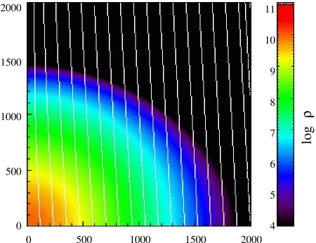
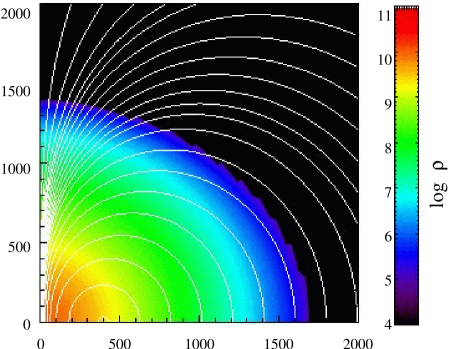
Figure 1: Logarithm of the rest mass density ($\log{\rho}$, color coded) and magnetic field lines ($B^{i}$, white curves) in a homogeneous $B^{*\,i}$ field configuration (left panel) and a magnetic field generated by a circular current loop (right panel), for a typical rotating iron core (model A1B3 in Table 1) used for the collapse simulations. The magnetic field lines have been calculated as isocontours of the vector potential. The axis scale is in km and the density in cgs units.

The initial magnetic field configuration is denoted in the names of the models in our sample by adding a label to the purely hydrodynamic model. For the latter we follow the notation of Dimmelmeier et al. (2002a) and Ott et al. (2007a). These models are listed in Table 1. The label for the magnetic field is constructed following the notation of Obergaulinger et al. (2006b). We add the suffix D3M0 to denote those models with purely poloidal magnetic field generated by a circular loop and $r_{\mathrm{mag}}=400\mathrm{\ km}$ (M0 denotes the passive field approximation) and we use the suffix T3M0 for models with purely toroidal magnetic field and $r_{\mathrm{mag}}=400\mathrm{\ km}$. We have also built the DT3M0 model, whose magnetic field distribution is a combination of D3M0 and T3M0 with equal magnetic field strengths at the center. This model allows us to check the validity of the “composition rule” (see Sect. 2.3).

3.2 Hydrodynamic configurations

3.2.1 Polytropes in rotational equilibrium

For the simulation with a simplified description of matter using the hybrid EOS (see Sect. 4.1), we construct $\gamma_{\mathrm{ini}}=4/3$ polytropes in rotational equilibrium which we obtain by using the relativistic generalization of Hachisu’s self-consistent field method by Komatsu et al. (1989). Their rotation law for the specific angular momentum $j$ is given by

$$j=A^{2}(\Omega_{\mathrm{c}}-\Omega),$$ (25)

where $A$ parametrizes the degree of differential rotation (stronger differentiality with decreasing $A$) and $\Omega_{\mathrm{c}}$ is the value of the angular velocity $\Omega$ at the center. In the Newtonian limit, this reduces to

$$\Omega=\frac{A^{2}\Omega_{\mathrm{c}}}{A^{2}+\varpi^{2}}.$$ (26)

The parameters of the selected models, which are chosen to be identical to some of the models considered by Dimmelmeier et al. (2002a), are described in Table 1. In addition, as we aim at comparing our results with the recent numerical simulations performed by Obergaulinger et al. (2006b) in Newtonian gravity, a subset of our models (those with purely poloidal magnetic field) have been selected as general relativistic counterparts of their models. In Table 1 we also give the values for the gravitational mass $M_{\mathrm{g}}$ (which is identical to the ADM mass $M_{\mathrm{ADM}}$) and for the initial rotation rate $\beta=E_{\mathrm{rot}}/|E_{\mathrm{b}}|$. In the definition of $\beta$ we use the following expressions for the rotational kinetic energy $E_{\mathrm{rot}}$, the gravitational binding energy $E_{\mathrm{b}}$, and the magnetic energy $E_{\mathrm{mag}}$:

$$E_{\mathrm{rot}} = \frac{1}{2}\int\mathrm{d}^{3}\mbox{\boldmath$x$}\,\sqrt{\gamma}\,\alpha\hat{v}^{\varphi}S_{\varphi},$$ (27)

$$E_{\mathrm{b}} = M_{\mathrm{g}}-M_{\mathrm{p}}-E_{\mathrm{rot}}-E_{\mathrm{mag}},$$ (28)

$$E_{\mathrm{mag}} = \frac{1}{2}\int\mathrm{d}^{3}\mbox{\boldmath$x$}\,\sqrt{\gamma}\,Wb^{2},$$ (29)

where $M_{\mathrm{p}}$ is the proper mass.

Table 1: Purely hydrodynamic initial models used in the magnetized core collapse simulations.

Model	$\rho_{\mathrm{c}}$	$A$	$\beta$	$M_{\mathrm{g}}$	$\gamma_{1}$
	[$10^{10}\mathrm{\,g\,cm}^{-3}$]	[$10^{3}\mathrm{\ km}$]	[%]	[$M_{\odot}$]
A1B3G3	1.00	50.0	0.90	1.46	1.300
A1B3G5	1.00	50.0	0.90	1.46	1.280
A3B3G5	1.00	0.5	0.90	1.46	1.280
A2B4G1	1.00	1.0	1.80	1.50	1.325
A4B5G5	1.00	0.5	4.00	1.61	1.280
s20A1B1	0.88	50.0	0.25	1.58	—
s20A1B5	0.88	50.0	4.00	1.58	—
s20A2B2	0.88	1.0	0.50	1.58	—
s20A2B4	0.88	1.0	1.80	1.58	—
s20A3B3	0.88	0.5	0.90	1.58	—
E20A	0.42	—	0.37	2.00	—

For these simplified initial models the gravitational collapse is initiated by slightly decreasing the adiabatic index from its initial value to $\gamma_{1}<\gamma_{\mathrm{ini}}=4/3$, which results in a loss of pressure support. If no pressure reduction were imposed, the purely hydrodynamic initial models would remain stationary. However, even in that case the associated initial magnetic field may not remain stationary (see also Table 2 below). Only a purely toroidal initial magnetic field would not evolve in time, while any magnetic field configuration of initial models labeled A1 would still stay approximately stationary, since these models rotate almost rigidly, and thus the initial magnetic field cannot wind up itself strongly.

3.2.2 Presupernova models from stellar evolution calculations

As initial models for the simulations where we use a microphysical EOS and deleptonization, we employ the solar-metallicity $20\,M_{\odot}$ (zero-age main sequence) model of Woosley et al. (2002) (labeled as model s20 in Table 1). On this spherically symmetric model, which is initially not in equilibrium as it has a non-zero radial velocity profile, we impose the rotation law (25), using the same rotation nomenclature as for the previously described polytropes in equilibrium.

In addition, we perform calculations with the “rotating” presupernova model E20A of Heger et al. (2000), which we map onto our computational grids under the assumption of constant rotation on cylindrical shells of constant $\varpi$.

4 Treatment of matter during the evolution

In this work we improve upon preceding relativistic stellar core collapse simulations by using an advanced description of microphysics as presented in Ott et al. (2007a) and Dimmelmeier et al. (2007a). For comparison to previous results, we also perform simulations with the simplified hybrid EOS (Janka et al. 1993). In the following, we describe both approaches for the treatment of matter.

4.1 Hybrid EOS

For calculations employing polytropes in rotational equilibrium as initial models, we utilize the hybrid EOS. Here the pressure consists of a polytropic part, $P_{\mathrm{p}}=K\rho^{\gamma}$, with $K=4.897\times 10^{14}$ (in cgs units), plus a thermal part, $P_{\mathrm{th}}=\rho\epsilon_{\mathrm{th}}(\gamma_{\mathrm{th}}-1)$, where $\epsilon_{\mathrm{th}}=\epsilon-\epsilon_{\mathrm{p}}$ and where we set $\gamma_{\mathrm{th}}=1.5$. The thermal contribution is chosen to take into account the rise of thermal energy due to shock heating. As $\rho$ reaches nuclear density at $\rho_{\mathrm{nuc}}=2.0\times 10^{14}\mathrm{\ g\ cm}^{-3}$, $\gamma$ is raised to $\gamma_{2}=2.5$ and $K$ adjusted accordingly to maintain monotonicity of $P$ and $\epsilon$. Due to this stiffening of the EOS the core undergoes a so-called pressure-supported bounce. More details of the hybrid EOS can be found e.g. in Dimmelmeier et al. (2002a).

4.2 Microphysical EOS, deleptonization scheme, and neutrino pressure

In our more realistic calculations, for which the models s20 and E20A from stellar evolution are taken as initial models, we employ the tabulated non-zero temperature nuclear EOS by Shen et al. (1998) in the variant of Marek et al. (2005) which includes baryonic, electronic, and photonic pressure components. This gives the fluid pressure $P$ (and additional thermodynamic quantities) as a function of $\rho$, the temperature $T$, and the electron fraction $Y_{e}$. Since the code operates with the specific internal energy $\epsilon$ instead of the temperature $T$, we determine the corresponding value for $T$ iteratively with a Newton–Raphson scheme.

To determine the evolution of $Y_{e}$, the state vector, flux vector, and source vector for the conservation equations (13), as given in Eqs. (14–16) have to be augmented by the components

$$DY_{e},\qquad DY_{e}\hat{v}^{i},\qquad S_{Y_{e}},$$ (30)

respectively. The source term $S_{Y_{e}}$ is a consequence of the electron captures during collapse, which reduces $Y_{e}$. This deleptonization also effectively decreases the size of the homologously collapsing inner core, and has thus a direct influence on the collapse dynamics and the gravitational wave signal. Hence, it is essential to include (at least an approximate scheme for) deleptonization during collapse.

Since multi-dimensional radiation hydrodynamics calculations in general relativity are not yet computationally feasible, in the simulations using the microphysical EOS we make use of a a recently proposed scheme (Liebendörfer 2005) where deleptonization is parametrized based on data from detailed spherically symmetric calculations with Boltzmann neutrino transport. As in Dimmelmeier et al. (2007a) we take the latest available electron capture rates (Langanke & Martínez-Pinedo 2000), which result in lower values for $Y_{e}$ in the inner core at bounce compared to recent results (Ott et al. 2007a) where standard capture rates were used (Rampp & Janka 2000). Following Liebendörfer (2005), deleptonization is stopped at core bounce (i.e. as soon as the specific entropy $s$ per baryon exceeds $3k_{\mathrm{B}}$). After core bounce $Y_{e}$ is only passively advected, neglecting any further deleptonization in the nascent PNS.

Neutrino pressure is included only in the regime which is optically thick to neutrinos, which we define for $\rho$ being above the trapping density $\rho_{\mathrm{t}}=2\times 10^{12}\mathrm{\ g\ cm}^{-3}$. Following Liebendörfer (2005), here we approximate the contribution of the neutrino pressure $P_{\nu}$ as an ideal Fermi gas and include the radiation stress via additional source terms in the momentum and energy equations for the fluid.

5 Outline of the numerical approach

The GRMHD numerical code we use in our simulations is based on the purely hydrodynamic code described in Dimmelmeier et al. (2002a, b), and on its extension discussed in Cerdá-Durán et al. (2005). It has been described in detail in a previous paper (Cerdá-Durán & Font 2007), which allows us to provide here only succint information. The code performs the coupled time evolution of the equations governing the dynamics of the spacetime, the fluid, and the magnetic field in general relativity. The equations are implemented in the code using spherical polar coordinates $\{t,r,\theta,\varphi\}$, assuming axisymmetry with respect to the rotation axis and equatorial plane symmetry at $\theta=\pi/2$.

5.1 The hydrodynamics solver

For the evolution of the matter fields we utilize a high-resolution shock-capturing (HRSC) scheme, which numerically integrates the subset of equations in system (13) that corresponds to the purely hydrodynamic variables ($D$, $S_{i}$, $\tau$). HRSC methods ensure the numerical conservation of physically conserved quantities and a correct treatment of discontinuities such as shocks (see e.g. Font 2003, for a review and references therein). We have implemented in the code various cell-reconstruction procedures, either second-order or third-order accurate in space, namely minmod, MC, and PHM (see Toro 1999, for definitions). The time update of the state vector $U$ is done using the method of lines in combination with a second-order accurate Runge–Kutta scheme. The numerical fluxes at the cell interfaces are obtained using either the HLL single-state solver of Harten et al. (1983) or the symmetric scheme of Kurganov & Tadmor (2000) (KT hereafter). Both solvers yield results with an accuracy comparable to complete Riemann solvers (with the full characteristic information), as shown in simulations involving purely hydrodynamic special relativistic flows (Lucas-Serrano et al. 2004) and general relativistic flows in dynamical spacetimes (Shibata & Font 2005). Tests of both solvers in GRMHD have been reported recently by Antón et al. (2006).

5.2 Evolution of the magnetic field

The evolution of the magnetic field needs to be performed in a way that is different from the rest of the conservation equations, since the physical meaning of the corresponding conservation equation is different. Although the induction equation can be written in a flux conservative way, a supplementary condition for the magnetic field has to be given (the divergence constraint), which has to be fulfilled at each time iteration. The physical meaning of these two equations is the conservation of the magnetic flux in a close volume, in our case each numerical cell. Therefore, an appropriate numerical scheme has to be used which takes full profit of such a conservation law. Among the numerical schemes that satisfy this property (see Tóth 2000, for a review), the constrained transport (CT) scheme (Evans & Hawley 1988) has proved to be adequate to perform accurate simulations of magnetized flows. Our particular implementation of this scheme (see Cerdá-Durán & Font 2007, for details) has been adapted to the spherical polar coordinates used in the code. The discretized evolution equations for the poloidal components of the magnetic field read

$$\partial_{t}B^{*\,r}_{i+{1\over 2}\,j} = \frac{[\sin\theta\,E^{*}_{\varphi}]_{i+{1\over 2}\,j+{1\over 2}}-[\sin\theta\,E^{*}_{\varphi}]_{i+{1\over 2}\,j-{1\over 2}}}{r_{i+{1\over 2}\,j}\,\Delta(\cos\theta)_{j}},$$ (31)

$$\partial_{t}B^{*\,\theta}_{i\,j+{1\over 2}} = 2\,\frac{[r\,E^{*}_{\varphi}]_{i+{1\over 2}\,j+{1\over 2}}-[r\,E^{*}_{\varphi}]_{i-{1\over 2}\,j+{1\over 2}}}{\Delta r^{2}_{i}},$$ (32)

where (in vectorial form) $\mbox{\boldmath$E$}^{*}=\mbox{\boldmath$v$}^{*}\times\mbox{\boldmath$B$}^{*}$, and where cell centers are located at $(i\,j)$, radial interfaces at $(i+{1\over 2}\,j)$, angular interfaces at $(i\,j+{1\over 2})$, and cell corners (cell edges along the $\varphi$-direction) at $(i+{1\over 2}\,j+{1\over 2})$. We note that the evolution equation for the toroidal magnetic field is analog to that used for the hydrodynamics, since in axisymmetry this component does not play any role in the CT scheme. The previous expressions are used in the numerical code to update the magnetic field. The only remaining aspect is to give an explicit expression for the value of $E^{*}_{i}$. A practical way to calculate $E^{*}_{\varphi}$ from the numerical fluxes in the adjacent interfaces (Balsara & Spicer 1999) is

$$E^{*}_{\varphi\,i+{1\over 2}\,j+{1\over 2}} = -\frac{1}{4}\left[(F^{r})^{\theta}_{i\,j+{1\over 2}}+(F^{r})^{\theta}_{i+1\,j+{1\over 2}}\right.$$ (33)

$$\left.\qquad-(F^{\theta})^{r}_{i+{1\over 2}\,j}-(F^{\theta})^{r}_{i+{1\over 2}\,j+1}\right],$$

where the fluxes (15) are obtained in the usual way by solving the Riemann problem at the interfaces. The combination of the CT scheme and this way of computing the electric field is called the flux-CT scheme. It is used in all numerical simulations reported in this paper. Finally, the time discretization of Eqs. (31) and (32) is performed in the same way as for the fluid evolution equations.

5.3 The metric solver

The CFC metric equations are five nonlinear elliptic coupled Poisson-like equations which can be written in compact form as $\hat{\Delta}\mbox{\boldmath$u$}(\mbox{\boldmath$x$})=\mbox{\boldmath$f$}(\mbox{\boldmath$x$};\mbox{\boldmath$u$}(\mbox{\boldmath$x$}))$, where $\mbox{\boldmath$u$}=u^{k}=(\phi,\alpha\phi,\beta^{j})$, and $\mbox{\boldmath$f$}=f^{k}$ is the vector of the respective sources. These five scalar equations for each component of $u$ couple to each other via the source terms that in general depend on the various components of $u$. We use a fix-point iteration scheme in combination with a linear Poisson solver to solve these equations. Further details on this type of metric solver can be found in Cerdá-Durán et al. (2005) and Dimmelmeier et al. (2002a).

5.4 Setup of the numerical grid

Table 2: Hydrodynamical and magnetic field properties of all models computed in this work. From left to right the columns report the name of the model, the stationarity properties of the initial magnetic field, the maximum rest-mass density $\rho_{\mathrm{max}}$, the maximum poloidal field $|B_{\mathrm{polo}}|_{\mathrm{max}}$, the maximum toroidal field $|B_{\varphi}|_{\mathrm{max}}$, the rotational energy parameter $\beta_{\mathrm{rot}}$, the magnetic energy parameter $\beta_{\mathrm{mag}}$, its poloidal contribution $\beta_{\mathrm{polo}}$, and the central angular velocity $\Omega_{\mathrm{c}}$. The time scale $\tau_{\Omega}$ of the growth of the magnetic field by the $\Omega$-dynamo and the saturation time $t_{\mathrm{sat}}$ for this process are also shown.

Model	stationary	$\rho_{\mathrm{max}}$	$|B_{\mathrm{polo}}|_{\mathrm{max}}$	$|B_{\varphi}|_{\mathrm{max}}$	$\beta_{\mathrm{rot}}$	$\beta_{\mathrm{mag}}$	$\beta_{\mathrm{polo}}$	$\Omega_{\mathrm{c}}$	$\tau_{\Omega}$	$t_{\mathrm{sat}}$
		$\displaystyle\left[10^{14}\frac{\mathrm{g}}{\mathrm{\ cm}^{3}}\right]$	[$10^{10}\mathrm{\ G}$]	[$10^{10}\mathrm{\ G}$]	[$10^{-2}$]	[$10^{-8}$]	[$10^{-8}$]	[$\mathrm{ms}^{-1}$]	[s]	[s]
A2B4G1-D3M0	no	0.47	400	1467	15.6	8.3	0.9	0.36	85	10.3
A1B3G3-D3M0	approx.	4.22	1719	2522	2.3	1.2	0.8	3.96	7	0.3
A1B3G3-T3M0	yes	4.22	0	1714	2.3	0.2	0.0	3.96	—	—
A1B3G5-D3M0	approx.	4.57	1146	1275	0.9	0.5	0.4	3.91	21	0.7
A1B3G5-T3M0	yes	4.57	0	1542	0.9	0.2	0.0	3.91	—	—
A1B3G5-DT3M0	approx.	4.57	1146	1537	0.9	0.6	0.4	3.91	21	0.6
A3B3G5-D3M0	no	3.73	984	1672	2.3	0.6	0.4	3.75	24	1.1
A4B5G5-D3M0	no	1.74	1094	2716	8.5	4.4	1.2	1.18	24	2.1
A4B5G5-T3M0	yes	1.74	0	1626	8.5	0.4	0.0	1.18	—	—
s20A1B1-D3M0	approx.	2.69	1221	162	0.6	2.9	2.9	1.34	22	0.5
s20A2B2-D3M0	no	2.75	1849	3574	5.8	7.6	3.2	3.55	7	0.5
s20A2B2-T3M0	yes	2.75	0	1365	5.8	0.9	0.0	3.55	—	—
s20A1B5-D3M0	approx.	2.69	1100	1011	7.8	3.2	2.4	3.89	10	0.8
s20A1B5-T3M0	yes	2.69	0	1447	7.8	1.2	0.0	3.89	—	—
E20A-D3M0	no	2.29	2343	7503	7.7	23.4	1.8	4.37	6	0.5
E20A-T3M0	yes	2.29	0	2739	7.7	1.9	0.0	4.37	—	—

We perform all axisymmetric simulations with a resolution ($n_{r}\times n_{\theta}$) of $300\times 30$ zones, except for models labeled A4B5G5 in which a resolution of $300\times 40$ is used due to the more complex angular structure. In both cases the radial grid is equally spaced for the first 100 points, with a grid spacing of $100\mathrm{\ m}$. The remaining radial zones are logarithmically distributed to cover the outer parts of the star and the exterior artificial low-density atmosphere. The angular grid is equally spaced and we assume equatorial symmetry. We have performed resolution tests and we have found that such a resolution is adequate for our simulations (see Cerdá-Durán 2006; Cerdá-Durán & Font 2007, for details). As a consequence of our various code tests (see Appendix A) all results discussed in Sect. 6 correspond to simulations performed using PHM reconstruction and the HLL solver for the hydrodynamics.

6 Results

We now present the main results from our numerical simulations of rotational magnetized core collapse to neutron stars. First, we note that a quantitative summary of our findings is reported in Table 2, to which we will refer repeteadly. The dynamics of the models we have selected is identical to the dynamics of the unmagnetized ones, since the passive field approximation is used. Therefore, we will not describe here all the morphological features of the hydrodynamics of both models with the hybrid EOS (simplified models hereafter) and models with the microphysical EOS and the deleptonization scheme (microphysical models hereafter), as they have been discussed in detail in Dimmelmeier et al. (2002a, b), and Ott et al. (2007b) as well as Dimmelmeier et al. (2007a, b), respectively. (It is worth to emphasize, however, the excellent agreement found in the hydrodynamical simulations performed with three independent numerical codes.) We pay more attention instead to the magnetic field evolution. In all our simulations an initial magnetic field strength of $B^{*}_{0}=10^{10}\mathrm{\ G}$ is considered. This value is an upper limit for the T3M0 models, since the expected initial toroidal magnetic field is of this order (Heger et al. 2005). However, for the D3M0 models, this field strength is already at (or above) the upper end of the astrophysically expected values.

For all models we first present results for identical values of $B^{*}_{0}$, in a way that we can study the different effects and compare them properly. Afterwards we present the results scaled to lower, astrophysically expected values. We anticipate that our results can change if some of the several assumptions made in our simulations (axisymmetry and passive field approximation) are relaxed. An estimation and discussion of these effects can be found in Sect. 6.6.

6.1 Evolution of the magnetic energy parameter

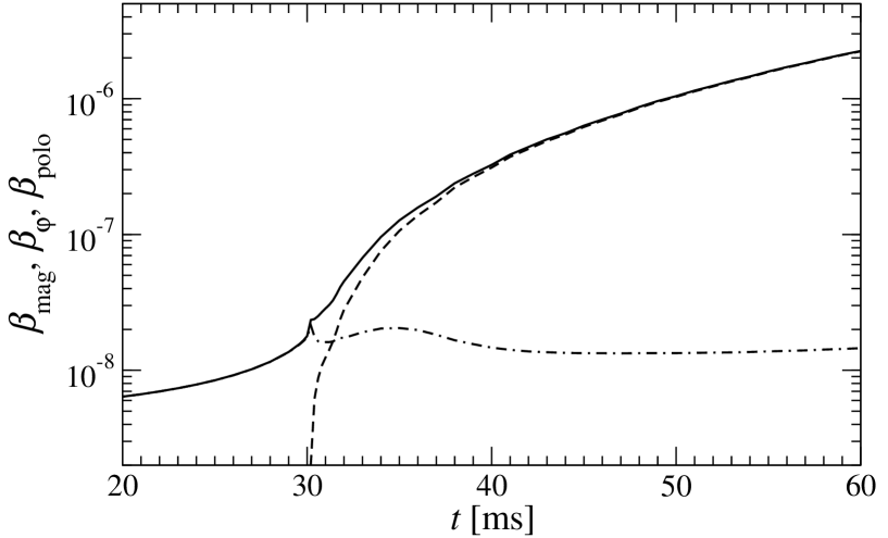
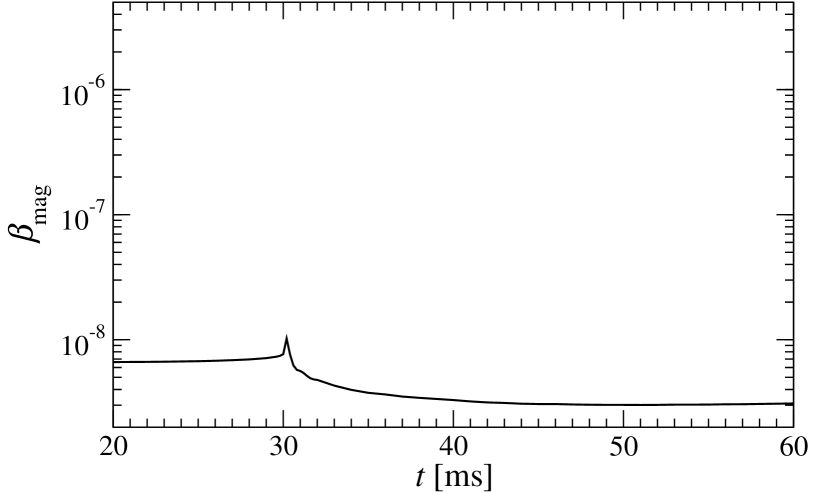
Figure 2: Time evolution of the magnetic energy parameters $\beta_{\mathrm{mag}}$ (solid line), $\beta_{\varphi}$ (dashed line), and $\beta_{\mathrm{polo}}$ (dashed-dotted line) for models A1B3G5-D3M0 (top panel) and A1B3G5-T3M0 (bottom panel).

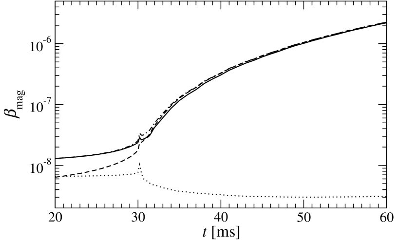
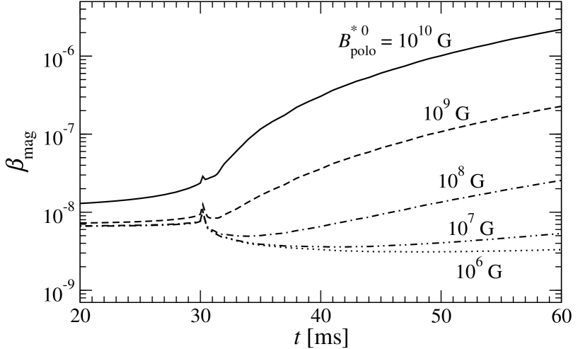
Figure 3: Time evolution of the magnetic energy parameter $\beta_{\mathrm{mag}}$. The top panel shows $\beta_{\mathrm{mag}}$ for model A1B3G5-DT3M0 (solid line) and the comparison with the composition (dot-dashed line) of models A1B3G5-D3M0 (dashed line) and A1B3G5-T3M0 (dotted line). The bottom panel shows the evolution of $\beta_{\mathrm{mag}}$ for the same hydrodynamic model (A1B3G5) with an initial value of the toroidal field of $B^{*\,0}_{\varphi}=10^{10}\mathrm{\ G}$, and varying values of the initial poloidal field $B^{*\,0}_{\mathrm{polo}}$, from $10^{6}$ to $10^{10}\mathrm{\ G}$.

The evolution of the energy parameter for the magnetic field $\beta_{\mathrm{mag}}=E_{\mathrm{mag}}/|E_{\mathrm{b}}|$ can be seen in Fig. 2 for model A1B3G5 of our sample. In order to analyze the amplification of the magnetic field, we separate the effects of the different components of the magnetic field into $\beta_{\varphi}$ for the toroidal component and $\beta_{\mathrm{polo}}=\beta_{\mathrm{mag}}-\beta_{\varphi}$ for the poloidal component, which are also plotted in the figure. As the collapse proceeds the magnetic field grows by at least two reasons: First, the radial flow compresses the magnetic field lines, amplifying the existing poloidal and toroidal magnetic field components. Second, during the collapse of a rotating star differential rotation is produced and increased, even for rigidly rotating initial models (see e.g. Dimmelmeier et al. (2002b)). Hence, if a seed poloidal field exists, the $\Omega$-dynamo mechanism winds up the poloidal field lines into a toroidal component. This (linear) amplification process generates a toroidal magnetic field component, even from purely poloidal initial configurations. The toroidal component of the magnetic field is affected by the two effects, while the poloidal field is only amplified by radial compression of the field lines. Thus, even if the initial magnetic field configuration is purely poloidal, the toroidal component dominates after some dynamical time. To study the differences in the evolution of the magnetic field depending on the initial magnetic field we now describe in detail the features of model A1B3G5 with different initial magnetic field configurations.

In model A1B3G5-D3M0 the initial magnetic field is entirely poloidal. The top panel of Fig. 2 shows that $\beta_{\varphi}$ (dashed line) grows much faster than $\beta_{\mathrm{polo}}$, particularly after bounce ($t\sim 30\mathrm{\ ms}$) when the radial compression mechanism stops. We note that the magnetic field considered is weak enough not to affect the dynamics, with the final $\beta_{\mathrm{mag}}\ll 1$.

If we consider a purely toroidal magnetic field initially, as model A1B3G5-T3M0, the only amplification mechanism present in our simulations is the radial compression, since no poloidal field can be wound up. The bottom panel of Fig. 2 shows the behaviour of $\beta_{\mathrm{mag}}$ for model A1B3G3-T3M0. It is important to notice that during the collapse $\beta_{\mathrm{mag}}$ hardly grows (for other models of the T3M0 series it even decreases) since the radial compression is a very inefficient mechanism to amplify the magnetic field. As a result, for some models the final PNS is “less magnetized” than the progenitor core in the sense that $\beta_{\mathrm{mag}}$ at bounce is smaller than it is before the collapse. We note that the evolution of this kind of purely toroidal models could change completely if the axisymmetry condition were removed, since in three dimensions there are mechanisms that can transform a toroidal magnetic field into a poloidal one. Some of these mechanisms are discussed in Sect. 6.6 below.

To check whether the “composition rule” (see Sect. 2.3) is valid we consider next a mixed configuration of poloidal and toroidal magnetic fields at the beginning of the simulation (model A1B3G5-DT3M0). The top panel of Fig. 3 shows with a solid line the time evolution of $\beta_{\mathrm{mag}}$ for model A1B3G5-DT3M0 and with a dot-dashed line the composition of the individual values for $\beta_{\mathrm{mag}}$ in models A1B3G5-D3M0 and A1B3G5-T3M0 with identical initial field strengths. (The separate evolutions for the latter are also included in the plot as dashed and dotted lines, respectively.) The agreement of the two evolution paths is remarkable, which shows that the “composition rule” works properly for our simulations. Therefore, we can use it to obtain any desirable composition of magnetic fields with a single hydrodynamic evolution of the two models D3M0 and T3M0. For the particular composition showed in this model, the final value of $\beta_{\mathrm{mag}}$ depends very weakly on the initial toroidal magnetic field component. In other words, the structure of the magnetic field of the PNS will depend almost exclusively on the radial compression of the initial poloidal component of the magnetic field.

Next, we consider a “composition” of these models with different initial magnetic field strength. We keep the initial toroidal component fixed at a realistic value, $B^{*\,0}_{\varphi}=10^{10}\mathrm{\ G}$, and change the initial poloidal component in a range that spans from $B^{*\,0}_{\mathrm{polo}}=10^{10}\mathrm{\ G}$ down to the astrophysically more realistic value of $10^{6}\mathrm{\ G}$. The bottom panel of Fig. 3 shows the time evolution of $\beta_{\mathrm{mag}}$ for these different configurations. For lower values of $B^{*\,0}_{\mathrm{polo}}$, the $\Omega$-dynamo mechanism becomes increasingly slower and the initial toroidal component becomes important for the magnetic field configuration of the PNS. In the lowest initial poloidal field case analyzed, the magnetic field of the PNS is completely toroidal and depends exclusively on the initial magnetic field configuration.

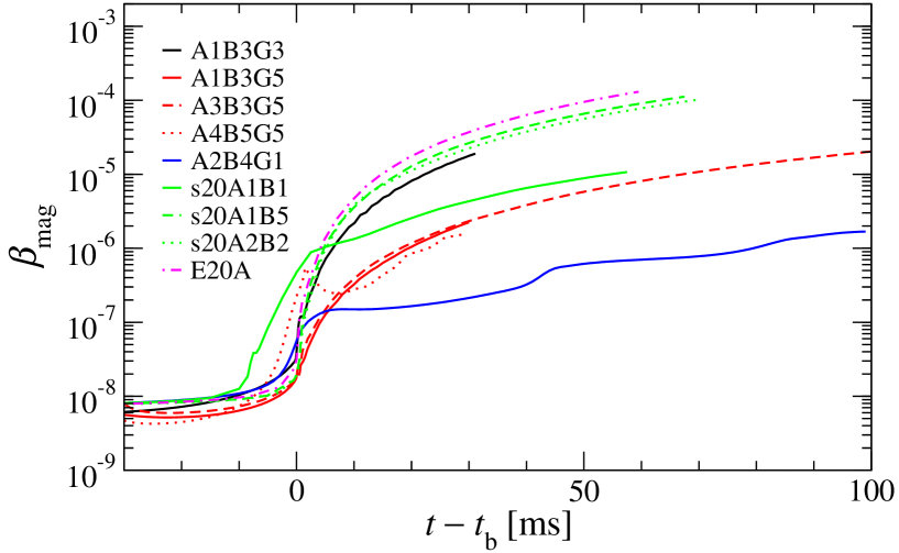
Figure 4: Time evolution of the magnetic energy parameter $\beta_{\mathrm{mag}}$ for all simulated models with initial purely poloidal magnetic field (label D3M0).

The remaining computed models of our sample, including those with microphysics, behave qualitatively in a very similar manner, although quantitative differences can be found in the amplification of the magnetic field during the collapse, and the amplification rates after bounce due to the $\Omega$-dynamo. Fig. 4 shows the evolution of the magnetic energy parameter $\beta_{\mathrm{mag}}$ for all the simulated models with initial purely poloidal magnetic field (label D3M0). For all models we find the following relation between the collapse time and the amplification rate of the magnetic field after bounce (which, however, does not hold for model A2B4G1-D3M0, as this is the only model of our sample for which the collapse is halted not by the stiffening of the EOS, but rather by centrifugal forces at subnuclear densities; cf. Dimmelmeier et al. 2002b): Models with large collapse times, such as all microphysical models as well as the simplified model A1B3G3-D3M0, exhibit a more efficient amplification of the magnetic field as compared to the rapid collapse models (G5 series). To quantify the differences between the models we estimate the time scale $\tau_{\Omega}$ for the amplification of the magnetic field by fitting the post-bounce evolution of $\beta_{\mathrm{mag}}$ to

$$\beta_{\mathrm{mag}}=\left(\frac{t}{\tau_{\Omega}}\right)^{2}.$$ (34)

The resulting values can be found in Table 2. The time scale should depend on the central angular velocity $\Omega_{\mathrm{c}}$ of the PNS, and on the strength of the poloidal magnetic field that can be wound up, which can be estimated from $\beta_{\mathrm{polo}}$. Hence, the following expression should be valid in the most efficient scenario (see Appendix B for details):

$$\tau_{\Omega}=\frac{2}{\Omega_{\mathrm{c}}\sqrt{\beta_{\mathrm{polo}}}}.$$ (35)

To check this relation we plot in the top panel of Fig. 5 the value of the fit for $\tau_{\Omega}$ versus the value from the previous analytic expression. Apparently for all models the growth time of the $\Omega$-dynamo is always larger than that of the most efficient situation (solid line in the figure), and corresponds to a fraction (30% – 90%) of the upper limit (35). This relation shows that in order to obtain higher amplification rates of the magnetic field not only strong rotation is needed, but also a sufficient compression of the poloidal magnetic field during the collapse.

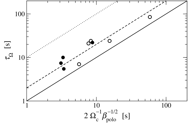
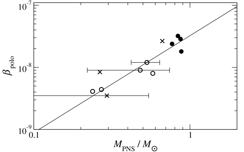
Figure 5: Top panel: relation between the fitted values for the growth time $\tau_{\Omega}$ of the $\Omega$-dynamo and the upper limit given by $2\,\Omega_{\mathrm{c}}^{-1}\beta_{\mathrm{polo}}^{-1/2}$. The solid line represents the upper limit, the dashed line corresponds to 50% of that limit, and the dotted line to 10%. Bottom panel: magnetic energy parameter $\beta_{\mathrm{polo}}$ of the poloidal component of the magnetic field at bounce versus the average mass $M_{\mathrm{PNS}}$ of the PNS after bounce, and its fit to a power law. Error bars are shown for models with mass variations larger than 5% after bounce. Both microphysical models (filled circles) and simplified models (open circles) are presented. Newtonian models (crosses) are also shown, but are not used in the fit.

Furthermore, we also find a relation between the value of $\beta_{\mathrm{polo}}$ and the mass enclosed in the neutrino sphere, $M_{\mathrm{PNS}}$ hereafter (see bottom panel of Fig. 5). Since most of the magnetic field lines compressed by the collapse are located inside the neutrino sphere, it is easy to understand that more massive PNS have higher magnetic energies. The fit to a power law of the data shown in Fig. 5 yields

$$\beta_{\mathrm{polo}} = (3.2\pm 0.5)\times$$ (36)

$$10^{-8}\left(\frac{M_{\mathrm{PNS}}}{M_{\odot}}\right)^{(1.6\pm 0.2)}\left(\frac{B^{*}_{0}}{10^{10}\mathrm{\ G}}\right)^{2}.$$

As discussed in detail by Dimmelmeier et al. (2007a, b), in the microphysical models the mass of the homologously collapsing inner core at bounce has a value of $\sim 0.5\,M_{\odot}$ (for the rotation rates considered here). This is also consistent with the high mass $M_{\mathrm{PNS}}\sim 0.8\,M_{\odot}$ of the PNS in these models, as shown in Fig. 5. To obtain masses in this range in models with a simple matter treatment, the adiabatic index would require a value $\gamma_{1}\gtrsim 1.32$, which is close to $4/3$. Already for moderate rotation, this choice would cause the core to undergo multiple centrifugal bounces at densities lower than nuclear density (as exemplified here in model A2B4G1), which is a dynamical behavior that does not occur at all in microphysical models (Dimmelmeier et al. 2007a, b, see also the related discussion in Sect. 6.5). Therefore, only the microphysical models feature a collapse to a PNS that has both high densities and is in addition comparably heavy. This combination, which cannot be realized with the simplified models, explains the higher growth rates of the magnetic field due to the $\Omega$-dynamo observed if improved microphysics is taken into account.

Combining Eqs. (35) and (36) we can establish an upper limit to the growth rate of the magnetic field due to the $\Omega$-dynamo using only hydrodynamic quantities, namely $\Omega_{\mathrm{c}}$ and $M_{\mathrm{PNS}}$, and the strength of the magnetic field in the progenitor, $B^{*}_{0}$. This limit is given by

$$\tau_{\Omega} = (11.18\pm 0.9)\times$$ (37)

$$\left(\frac{1\mathrm{\ ms}^{-1}}{\Omega_{\mathrm{c}}}\right)\left(\frac{M_{\odot}}{M_{\mathrm{PNS}}}\right)^{(0.8\pm 0.1)}\left(\frac{10^{10}\mathrm{\ G}}{B^{*}_{0}}\right)\mathrm{\ s}.$$

This relation can be very useful to estimate how fast the magnetic field grows in a collapsed star, under the assumption of a weak magnetic field and with a similar poloidal configuration in the progenitor, using data from purely hydrodynamical simulations (with no magnetic fields). As a proof of consistency and in order to assess the quality of this estimate we have computed $\tau_{\Omega}$ with this method. We find that in all cases the estimate is a lower limit for the actual value of $\tau_{\Omega}$ obtained from the numerical simulations and deviates by at most 30%.

6.2 Convection

One of the most important features that can affect the evolution of the magnetic field in stellar core collapse to a PNS is the presence of convection. We present here a detailed analysis of this effect in our simulations. Since in all of our models the magnetic field is weak, the discussion can be performed without considering its influence. We also note that due to the approximations made in our simulations, specifically the lack of a consistent neutrino transport scheme, our findings regarding convection should not be considered as definite.

The stability conditions for a rotating star are given by the so-called Solberg–Høiland criteria (Tassoul 1978),

$$\begin{array}[]{rcl}\mathcal{C}_{\mathrm{SH1}}&=&\mbox{\boldmath$g$}\cdot{\bf\mathcal{B}}+\mathcal{J}\cdot\nabla\varpi>0,\\[1.99997pt] \mathcal{C}_{\mathrm{SH2}}&=&(\mbox{\boldmath$g$}\times\nabla\varpi)(\mathcal{B}\times\mathcal{J})>0,\end{array}$$ (38)

where $g$ is the gravitational acceleration, and the buoyancy and rotational terms are respectively given by

$$\mathcal{B}=\frac{\nabla\rho}{\rho}-\frac{\nabla P}{P\Gamma_{1}},\qquad\mathcal{J}=\frac{1}{\varpi^{3}}\nabla(\Omega^{2}\varpi^{4}),$$ (39)

with $\Gamma_{1}=(\partial\ln P/\partial\ln\rho)_{s,Y_{e}}$. Note that in the first condition of Eq. (38), $N^{2}=\mbox{\boldmath$g$}\cdot\mathcal{B}$ is the Brunt–Väisälä frequency and $\kappa^{2}=\mathcal{J}\cdot\nabla\varpi$ is the epicyclic frequency. In the case of either no rotation or uniform rotation the Solberg–Høiland criteria reduce to the well known Schwarzschild criterion, $N^{2}>0$. If one of the two conditions is not satisfied, convective instability develops. Following Miralles et al. (2004), the time scale of the fastest growing mode can be computed as

$$\tau_{\mathrm{\,SH}}=\operatorname{Im}\left[\left(\frac{\mathcal{C}_{\mathrm{SH1}}}{2}-\frac{1}{2}\sqrt{\mathcal{C}^{2}_{\mathrm{SH1}}-4\,\mathcal{C}_{\mathrm{SH2}}}\right)^{-1/2}\right].$$ (40)

It is very useful to express the buoyancy terms in the conditions (38) in terms of the contributions of the entropy and electron fraction gradients,

$$\mathcal{B}=\xi\,\nabla s+\delta\,\nabla Y_{\mathrm{e}},$$ (41)

with $\xi=-\partial\ln P/\partial s|_{\rho,Y_{e}}/\Gamma_{1}$ and $\delta=-\partial\ln P/\partial Y_{e}|_{\rho,s}/\Gamma_{1}$. We point out that the Solberg–Høiland criteria are valid exactly only in Newtonian gravity, and thus we use them here only as estimates. In order to assess the influence of general relativistic corrections, we also evaluate Eq. (38) using covariant derivatives with respect to the CFC metric, which yields very similar results. Note also that the Solberg–Høiland criteria are based on a local instability analysis, while the convection observed in our simulations covers extended regions.

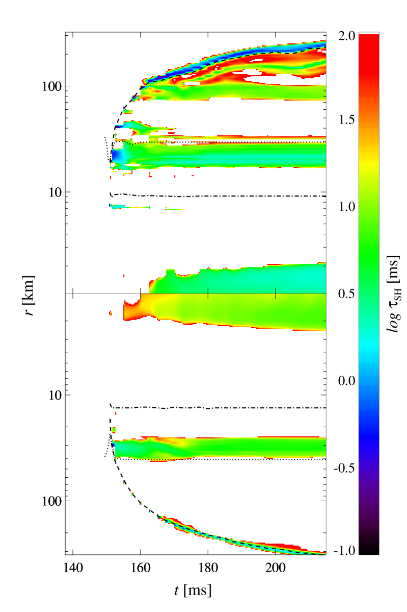
Figure 6: Time evolution of the angular averaged value of the growth time scale $\tau_{\mathrm{\,SH}}$, which indicates convectively unstable regions according to the Solberg–Høiland criteria. White regions represent convectively stable regions. The top half of the figure shows angular averages near the pole ($0<\theta<\pi/6$), while the bottom half shows the corresponding averages near the equator ($\pi/3<\theta<\pi/2$). The shock radius (dashed lines), neutrino sphere radius (dotted line), and radius of shock formation (dash-dotted line) are also displayed.

In Fig. 6 we show the extent of the convectively unstable regions according to the Solberg-Høiland criteria (38) after core bounce for models of the series s20A1B5, by plotting the time evolution of angle-averaged values for the convective growth time scale $\tau_{\mathrm{\,SH}}$. From this figure it becomes apparent that two regions are susceptible to developing instabilities: the region just below the neutrino sphere (between about $20\mathrm{\ km}$ and $40\mathrm{\ km}$) and extended regions behind the shock. The innermost $2\mathrm{\ km}$ of the star are also convectively unstable, but we suspect that the small negative entropy gradient responsible of this unstable region is a numerical artifact of the inner boundary, related to the so-called wall heating effect commonly appearing in shock reflection experiments (Donat & Marquina 1996). In our simulations of models of the series s20A1B5, convective motions indeed occur in those unstable regions as predicted by the instability criteria, as well as in the surrounding regions due to overshooting. We also find that the time scale of the onset of the observed instability is correctly estimated by Eq. (40).

Below the neutrino sphere ($20\mbox{\--\,}40\mathrm{\ km}$), convection sets in inmediately after bounce, with typical maximum velocities of about $2\times 10^{4}\mathrm{\ km\ s}^{-1}$. The velocities progressively decrease until the end of the simulation (at about $65\mathrm{\ ms}$ after bounce) with average values around $100\mathrm{\ km\ s}^{-1}$, although convection does not disappear completely. Behind the shock ($100\mbox{\,--\,}200\mathrm{\ km}$), the typical convective velocities are of the order of $1000\mathrm{\ km\ s}^{-1}$, with maximum values in some regions of $10^{4}\mathrm{\ km\ s}^{-1}$. This magnitude remains until the end of the simulation.

For a more detailed analysis we separately evaluate the different contributions in the Solberg–Høiland criteria (38) with $\mathcal{B}$ in the form of Eq. (41). Since the radial gradient of $Y_{e}$ is positive (as deleptonization is stronger towards the center during the collapse), this has an stabilizing effect against convection. Similarly, rotation also suppresses convection, since the epicyclic frequency $\kappa^{2}$ is positive everywhere. Convective instability can thus only appear in regions with a sufficiently large negative radial entropy gradient. Such a gradient occurs in the region already swept by the shock front. Shock heating creates entropy most strongly close to the neutrino sphere at a radius of about $30\mathrm{\ km}$ (see Fig. 6), producing a steep gradient there $1\mathrm{\ ms}$ after core bounce. Behind the shock front, which then propagates to larger radii at lower densities and decelerates, another region with a negative gradient also appears. All our microphysical models show very similar qualitative behavior with some variations due to different angular momentum distribution and the description of matter.

In models with slower rotation (i.e. the s20A1B1 series), strong convection sets in immediately after the occurence of the negative entropy gradient close to the neutrino sphere. For models with very little rotation (which have not been considered in this work), such convective overturn is strong enough to be clearly visible in the post-bounce gravitational wave signal (Dimmelmeier et al. 2007a, b). Within about $20\mathrm{\ ms}$ after core bounce, convection has managed to smooth out the entropy gradient around the neutrino sphere, thus removing the condition for sustained convection. Accordingly, convection is strongly damped, the vortices disappear quickly, and the low-frequency contribution to the gravitational wave signal is no longer visible. This fast convective transient near the neutrino sphere has been observed in numerical simulations without any neutrino treatment (see e.g. Burrows & Fryxell 1992; Müller & Janka 1997), and also in simulations using a neutrino diffusion scheme (Swesty & Myra 2005), although in the latter case the time scale for damping of convection is shorter ($\sim 10\mathrm{\ ms}$) than in our case. However, in simulations including state-of-the-art Boltzmann neutrino transport (Müller et al. 2004), a few ms after core bounce no significant convection remains in this region, and no traces in the gravitational wave signal can be found. We attribute this disagreement with our results to the simplified neutrino treatment in our models, which cannot properly take into account the deleptonization of the PNS after core bounce. As the deleptonization of the PNS is initially strongest when the shock travels through the neutrino sphere, we expect the most significant inaccuracies of our formulation there. We therefore conclude that the convection over $\sim 20\mathrm{\ ms}$, which we observe in the neutrino sphere region, is an artifact that should disappear once a more realistic neutrino description is included.

In more rapidly rotating models, the stabilizing effect of rotation in the Solberg–Høiland criteria prevents the strong transient we find in the slowly rotating models from developing, and significantly weaker convection is present in this region. However, irrespective of rotation, convection vortices are formed behind the decelerating shock front. On post-bounce evolution times of several $10\mathrm{\ ms}$, the weak but persistent convection is unable to remove the entropy gradient behind the shock, except near the rotation axis, where the specific angular momentum is smaller, and convection is stronger.

Rotation also influences the shape of the convective cells. If the buoyancy terms in the Solberg–Høiland criteria (38) are much larger than the rotation terms, the convective cells show no preferred direction. We observe this feature particularly in models with slower rotation (the s20A1B1 series), and to a lesser degree also in other convectively unstable models in the first few ms after bounce. If the buoyancy terms are comparable in magnitude to the rotation terms, convection develops preferredly parallel to the rotation axis (see e.g. Miralles et al. 2004). This effect is present in our microphysical models at later phases, as the entropy gradient has already been partially smoothed out and the buoyancy terms have become smaller.

In contrast to the microphysical models, which show remarkable convection in the PNS and behind the shock front, models with a simplified matter treatment exhibit either no convection at all, or only close to the neutrino sphere (in the case of models of the A1B3G5 series). This is a consequence of using the hybrid EOS in the latter models, which is unable to properly decelerate the shock after core bounce and turn it into an accretion shock. Hence in these models the entropy gradient is mostly positive behind the shock.

6.3 Structure of the magnetic field

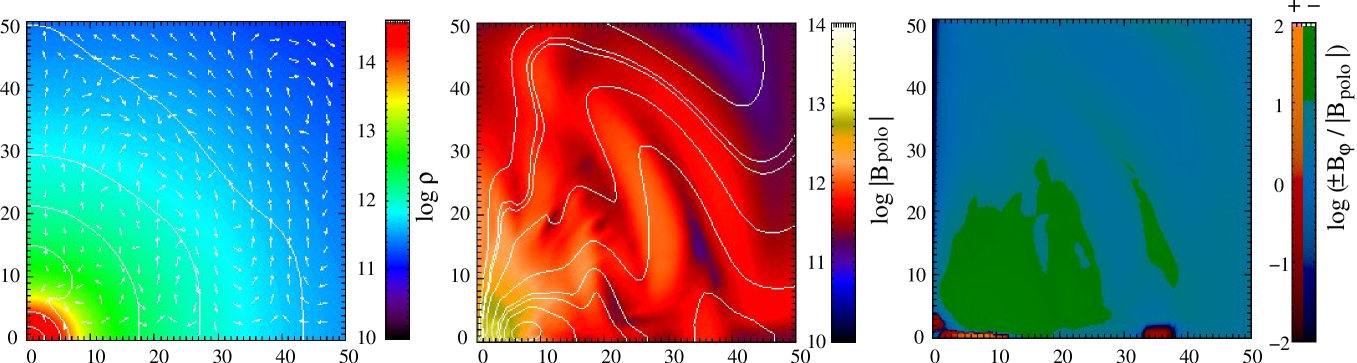
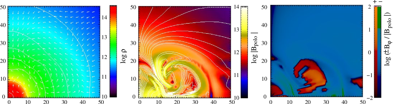
Figure 7: Configuration of the innermost region of the collapsed star at the end of the evolution for models A1B3G5-D3M0 (top panels; $t=60\mathrm{\ ms}$) and s20A1B1-D3M0 (bottom panels; $t=142.5\mathrm{\ ms}$). The left panels show the rest mass density as $\log\rho$ in units of $\mathrm{g\ cm}^{-3}$, overplotted by the meridional velocity field $(v^{r},v^{\theta})$ (arrows), and isocontours of the specific internal energy $\epsilon$. The center panels display the logarithm of the poloidal component of the magnetic field, $\log{|B_{\mathrm{polo}}|}$, in units of G and the magnetic field lines in the $r$–$\theta$ plane. The right panels show $B^{\varphi}/|B_{\mathrm{polo}}|$. All axes are in units of km.

The main qualitative differences between the various models become apparent when we study the detailed structure of the magnetic field of the resulting PNS. In Fig. 7 we show two-dimensional snapshots of selected hydrodynamic and magnetic field variables at the final time of the simulations for two representative models of our sample, namely model A1B3G5-D3M0 (top panels) and model s20A1B1-D3M0 (bottom panels). For typical simulations with initial poloidal magnetic fields (D3M0 models) the resulting PNS has two clearly distinct parts (see left panels of Fig. 7): an inner region with a size of $\sim 10\mathrm{\ km}$, where nuclear density is exceeded and which is almost rigidly rotating, and a surrounding shell extending to the neutrino sphere at $\sim 30\mathrm{\ km}$, with subnuclear densities and which is strongly differentially rotating. These two parts are also visible in the distribution of the magnetic field (see center and right panels of Fig. 7). The inner region has a mixed toroidal and poloidal magnetic field configuration, with both components having similar strength, which results in a helicoidal structure aligned with the rotation axis. As this part of the PNS is almost rigidly rotating and practically in equilibrium, the magnetic field hardly evolves in time. On the other hand, the outer shell is differentially rotating; thus the toroidal magnetic field component dominates and grows linearly with time due to the $\Omega$-dynamo mechanism.

If we compare the microphysical with the simplified simulations, we find that some significant morphological differences arise due to the stronger convection in the microphysical models just below the neutrino sphere. These motions affect the magnetic field, since they twist the poloidal magnetic field lines, generating a much more complicated structure of the poloidal field for those models. In particular those strong meridional currents distort the magnetic field in such a way that in some regions the poloidal component changes direction with respect to the rotation axis (see e.g. bottom-right panel of Fig. 7). This produces a negative effect in the $\Omega$-dynamo as in these regions the magnetic field is wound up in the opposite direction. However, the overall $\Omega$-dynamo mechanism seems not to be affected in a significant way by these local effects.

Model A4B5G5-D3M0 has to be discussed separately, since it has initially significantly stronger differential rotation and more angular momentum than the other models. As a result this model undergoes a core bounce due to centrifugal hang-up before reaching nuclear density. Its structure is toroidal with an off-center maximum density. Although it exhibits stronger differential rotation at the beginning compared to the other models, and the amplification process during collapse is thus more efficient, after bounce its angular velocity $\Omega$ is smaller (as the PNS is less compact) and therefore the linear amplification due to $\Omega$-dynamo is less pronounced. The main differences in the magnetic field structure of its PNS with respect to the other models are that, first, the $\Omega$-dynamo is active not only in the high-density torus, but also in the central lower-density region, and, second, the strong meridional currents twist the magnetic field lines around the torus. However, we point out that in the investigated range of initial rotation configurations all microphysical models are significantly less influenced by rotation than the simplified models (like A4B5G5), and that even for rather extreme rotation such collapse dynamics, leading to a toroidal structure, is strongly suppressed if an advanced description of microphysics is used (which is in accordance with the comprehensive parameter study by Dimmelmeier et al. 2007a).

In the models with initially purely toroidal field at the beginning (T3M0 series), a poloidal field cannot emerge in axisymmetry. Hence, the final magnetic field structure of the PNS consists of a stationary and entirely toroidal magnetic configuration with the highest field strengths found in the high density regions. As the rotational profile does not affect the distribution of the magnetic field, the different regions of the PNS are not visible in the structure of the magnetic field.

6.4 Comparison with Newtonian results

In order to study the general relativistic effects in the evolution of the magnetic field, we choose a subset of our simulations with the hybrid EOS to represent the relativistic version of some of the models of Obergaulinger et al. (2006a, b). Their first paper is devoted to Newtonian simulations of magneto-rotational core collapse, while in their second paper an effective relativistic gravitational potential was used to mimic general relativistic effects (while still keeping a Newtonian framework for the hydrodynamics; TOV models in their notation). Since in contrast to their work we use the passive field approximation, the comparison can only be made with the low magnetic field models presented in that work, namely the “M10” models. In these models the magnetic field does not affect the collapse dynamics and our approximation is valid. Although there are no qualitative differences between Newtonian and general relativistic models (aside from those coming purely from the hydrodynamics as described in Dimmelmeier et al. 2002a, b), some dissimilarities can be found in the magnetic field strength and amplification rates after core bounce.

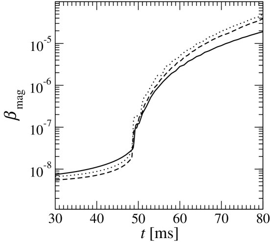
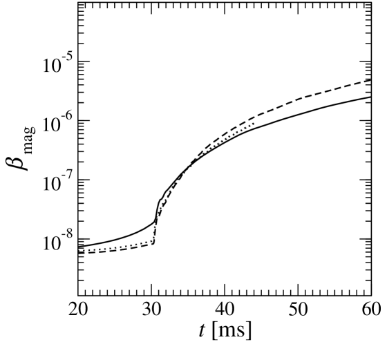
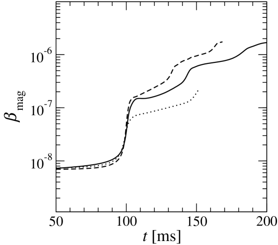
Figure 8: Comparison of the time evolution of the magnetic energy $E_{\mathrm{mag}}$ for models A1B3G3-D3M0 (left panel), A3B3G5-D3M0 (center panel) and A2B4G1-D3M0 (right panel). The line styles represent simulations performed in general relativity (solid lines), a purely Newtonian treatment (dotted lines), and Newtonian hydrodynamics with an effective relativistic TOV potential (dashed lines).

We have studied the evolution of the magnetic energy parameter $\beta_{\mathrm{mag}}$ for the various models, and plot the results in Fig. 8. Note that for the same initial magnetic field, the magnetic field contribution to the magnetic energy parameter differs between a purely Newtonian treatment, a Newtonian formulation with the effective relativistic TOV potential, and general relativity. As a consequence, the initial value of $\beta_{\mathrm{mag}}$ is not the same in these three cases. In order to be able to make an unambiguous comparison, we scale the magnetic fields such that $\beta_{\mathrm{mag}}$ in the initial model is equal to the value in general relativity. In general, for a similar hydrodynamic behavior (models A1B3G3-D3M0 and A3B3G5-D3M0) the magnetic energy attained during the evolution is smaller in the general relativistic case than in the Newtonian case (with either regular or effective relativistic TOV potential).

The winding up of magnetic field lines is the main mechanism responsible for the increase of the magnetic field during the collapse. Therefore the amplification rate for $\beta_{\mathrm{mag}}$ is determined by what rotation rate is reached and also by how strongly the poloidal component of the magnetic field is compressed. In the general relativistic case both higher densities and also stronger rotation are achieved (Dimmelmeier et al. 2002b). To investigate the impact of general relativistic gravity on the magnetic field compression, we consider $\beta_{\mathrm{polo}}$ as this quantity is the seed for the $\Omega$-dynamo. In general relativity the PNS has in general a smaller mass $M_{\mathrm{PNS}}$ than in the corresponding Newtonian simulation of the same model. Following the relation established in Sect. 6.1 (see the bottom panel of Fig. 5), the smaller PNS mass in the general relativistic simulation leads to a lower value of $\beta_{\mathrm{polo}}$. Therefore in that case, despite the larger $\Omega_{\mathrm{c}}$ the much smaller magnitude of $\beta_{\mathrm{polo}}$ results in a longer time scale for the $\Omega$-dynamo via Eq. (35), and hence a smaller growth rate of the magnetic field.

In the multiple centrifugal bounce model A2B4G1-D3M0, general relativistic effects lead to a bounce at significantly higher maximum densities than in Newtonian gravity. Therefore, this is the only investigated model where $M_{\mathrm{PNS}}$, and consequently $\beta_{\mathrm{polo}}$ as well as $\beta_{\mathrm{mag}}$ are larger in the general relativistic simulation.

6.5 Gravitational waves

We calculate the gravitational wave output from all of our simulations using the Newtonian quadrupole formula given in Eq. (22), which includes the magnetic terms. Thus, the quadrupole wave amplitude $A^{\mathrm{E2}}_{20}$, which is related to the dimensionless quadrupolar strain amplitude $h^{\mathrm{quad}}$ as

$$h^{\mathrm{quad}}=\frac{1}{8}\sqrt{\frac{15}{\pi}}\sin^{2}\theta\frac{A^{\mathrm{E2}}_{20}}{R},$$ (42)

contains the contribution $A^{\mathrm{E2}}_{\mathrm{20\,mag}}$ corresponding to the magnetic field. Here $h^{\mathrm{quad}}$ is the only independent component of the radiative part $h^{\mathrm{quad}}_{ij}$ of the spatial metric as given by Eq. (20). In order to understand how the magnetic field affects the waveforms, we also separately compute $A^{\mathrm{E2}}_{\mathrm{20\,mag}}$. The resulting waveforms for some representative models are shown in Fig. 9. As the magnetic field is very low at all times, $b^{2}\ll\rho$, the component of the gravitational wave due to the magnetic field is several orders of magnitude smaller than $A^{\mathrm{E2}}_{20}$.

Therefore, during the core bounce and the immediate post-bounce phase, the waveforms we obtain are practically identical to the ones presented for the same model setup in Dimmelmeier et al. (2002a) (for the simplified models) and Dimmelmeier et al. (2007a) (for the microphysical models), which can also be downloaded from a freely accessible waveform catalog at www.mpa-garching.mpg.de/rel_hydro/wave_catalog.shtml. The values for $A^{\mathrm{E2}}_{20}$ lie in the range between about $30\mathrm{\ cm}$ and $3000\mathrm{\ cm}$, which translates to a $h^{\mathrm{quad}}$ of roughly $3\times 10^{-22}$ to $3\times 10^{-20}$ (assuming a distance $R=10\mathrm{\ kpc}$ to the source and optimal orientation between the source and the detector).

We also emphasize that all investigated microphysical models yield gravitational wave signals known as Type I in the literature, i.e. the waveform exhibits a positive pre-bounce rise and then a large negative peak, followed by a ring-down. This is to be expected, as recent studies using the same hydrodynamical model setup (Ott et al. 2007a; Dimmelmeier et al. 2007a) have shown that the inclusion of microphysics in stellar core collapse simulations suppresses the other signal types, which were associated to multiple centrifugal bounce (Type II signals) or rapid collapse with a very small mass of the inner core (Type III signals).

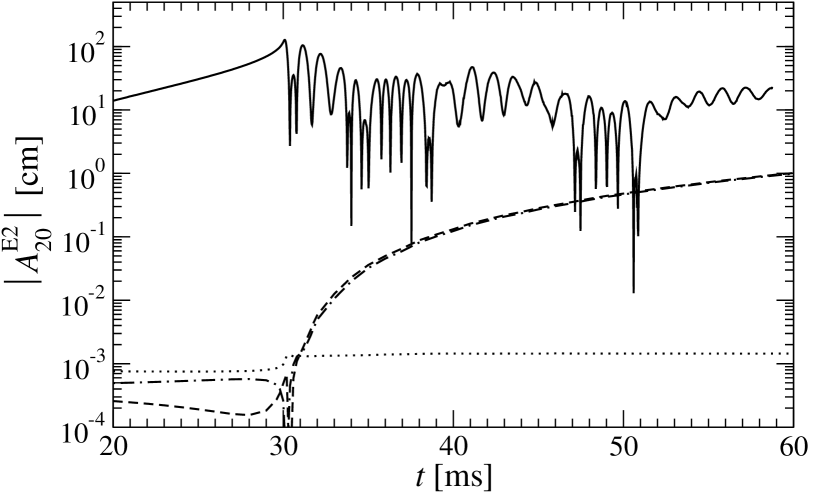
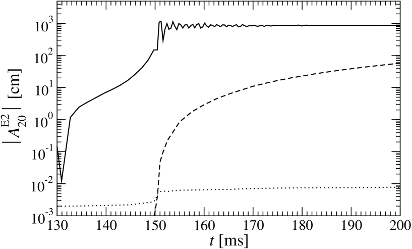
Figure 9: Absolute value of the gravitational wave amplitude $A^{\mathrm{E2}}_{20}$ (solid line) for models A1B3G5-D3M0/T3M0/DT3M0 (top panel) and s20A1B5-D3M0/T3M0 (bottom panel). For the low magnetic field strengths considered, the contribution of the magnetic field to the waveform is negligible, and the signals of series D3M0, T3M0, and DT3M0 are practically identical to the purely hydrodynamic waveform. For clarity, the component $A^{\mathrm{E2}}_{\mathrm{20\,mag}}$ from the magnetic field is also plotted for models A1B3G5-D3M0 (top panel, dashed line), A1B3G5-T3M0 (top panel, dotted line), A1B3G5-DT3M0 (top panel, dashed-dotted line), s20A1B5-D3M0 (bottom panel, dashed line), and s20A1B5-T3M0 (bottom panel, dotted line).

After bounce, the star reaches a quasi-equilibrium state, and thus, the hydrodynamic component of the waveform decreases. At the same time, for models D3M0, the magnetic field grows linearly with time. Such a behavior in the magnetic field produces an increasing gravitational wave signal, which grows quadratically with time due to the dependence on the magnetic field in Eq. (22). However, at the end of the simulation, the magnetic field component of the waveform is still negligible in comparison with the hydrodynamic component. It is expected that at later times, as the amplification of the magnetic field reaches saturation, the influence of the magnetic field on the waveform becomes significant, both due to its effect on the dynamics and also due to the contribution of the magnetic field to the gravitational radiation itself. We note, however, that the effect of the MRI could additionally lead to noticeable changes in the waveforms, provided it were able to efficiently amplify the magnetic field (see discussion in Sect. 6.6.2).

For models T3M0, on the other hand, the component of the waveform due to the magnetic field is even smaller than for the D3M0 models. This is a consequence of the inefficient amplification of the magnetic field via the radial compression. After bounce, the magnetic component of the waveforms in models T3M0 does not grow, and hence it is not expected to dominate the waveform later in the evolution, unless other processes amplifying the magnetic field were present.

6.6 Amplification of the magnetic field

Different mechanisms that amplify the magnetic field can act during a core collapse or the subsequent evolution of the newly formed PNS. This issue is of great importance, since the evolution of the PNS during its first minute of life until a cold NS forms can change drastically depending on the initial conditions at formation. One of the most important aspects is the distribution of angular momentum. A highly differentially rotating PNS can be subject to various types of instabilities, such as the dynamical low-$\beta$ instability, the classical bar-mode instability (which is unlikely to occur in a PNS on dynamical time scales as it requires very high values of $\beta$), or the secular CFS instability. Such instabilities are potential sources of detectable gravitational radiation. Therefore, a natural question that arises is whether the magnetic field is going to grow sufficiently fast to act on the PNS dynamics by flattening the rotation profiles (and therefore preventing the instabilities to develop), or whether, instead, the growth process may take a few seconds, allowing the instabilities to grow and the accompanying gravitational waves to become detectable. A number of effects can amplify the magnetic field shortly after PNS formation. In the following, we discuss these effects and estimate their importance for our models of core collapse.

6.6.1 $\Omega$-dynamo

Within our passive field approximation we can only compute the amplification rates for the $\Omega$-dynamo, for which the magnetic field grows linearly with time; therefore $\beta_{\mathrm{mag}}$ grows quadratically with time (see Appendix B). The time scale $\tau_{\Omega}$ of this amplification process and the estimated time $t_{\mathrm{sat}}$ at which the field saturation begins are given in Table 2. In the fastest case of our model sample, which occurs for model A1B3G3-D3M0, saturation is reached at about $300\mathrm{\ ms}$, and in most other cases, the $\Omega$-dynamo saturates at times larger than $0.5\mathrm{\ s}$. Note, however, that these estimates depend on the initial magnetic field strength, which is chosen to be $B^{*}_{0}=10^{10}\mathrm{\ G}$. For lower values of the magnetic field these time scales can be scaled as (see Eq. 54)

$$\tau_{\Omega}\approx\tau_{\Omega\,10}\left(\frac{10^{10}\mathrm{\ G}}{B^{*}_{0}}\right),\qquad t_{\mathrm{sat}}\approx t_{\mathrm{sat\,10}}\left(\frac{10^{10}\mathrm{\ G}}{B^{*}_{0}}\right).$$ (43)

We recall that stellar evolution calculations predict that in a progenitor core the poloidal component of the magnetic field can initially have a strength of about $10^{6}\mathrm{\ G}$ (Heger et al. 2005). For such an initial magnetic field the saturation time scale becomes several hours. This makes the $\Omega$-dynamo a very inefficient mechanism to amplify the magnetic field during core collapse and bounce, unless the progenitors are highly magnetized ($B>10^{10}\mathrm{\ G}$) for which the saturation could be reached within a few dynamical time scales. The magnetic field at the saturation is independent of the initial magnetic field strength and of the order of $\sim 10^{16}\mathrm{\ G}$.

6.6.2 Magneto-rotational instability

There are other magnetic field amplification processes that our simulations cannot account for, but for which it is nevertheless possible to estimate the growth rates. It has been suggested that the magneto-rotational instability could amplify the magnetic field from arbitrary weak fields up to values where equipartition between the magnetic field energy and the rotational kinetic energy is reached (Akiyama et al. 2003). However, our analysis shows that in the context of core collapse such an amplification is still an open issue. We proceed next to describe the MRI and the uncertainties related to its effect on the amplification of the magnetic field in core collapse.

Linear regime:

The MRI is a shear instability that generates turbulence and results in an amplification of the magnetic field in a differentially rotating magnetized plasma (Balbus & Hawley 1991, 1992), redistributing angular momentum in the plasma. Linear analysis shows that if the magnetic field strength is very low, as in our case, the stability criteria for the MRI in the Newtonian limit (Balbus 1995) are

$$\begin{array}[]{rcl}\mathcal{C}_{\mathrm{MRI1}}&=&\mbox{\boldmath$g$}\cdot{\bf\mathcal{B}}+\mathcal{R}\cdot\nabla\varpi>0,\\[1.99997pt] \mathcal{C}_{\mathrm{MRI2}}&=&(\mbox{\boldmath$g$}\times\nabla\varpi)(\mathcal{B}\times\mathcal{R})>0,\end{array}$$ (44)

where $\mathcal{R}=\varpi\nabla(\Omega^{2})$. Note that these criteria are very similar to the Solberg–Høiland criteria (38) for convection, but use an angular velocity gradient $\mathcal{R}$ instead of an angular momentum gradient $\mathcal{J}$. Since in the core collapse scenario $\mathcal{R}\leq 0$ is satisfied almost everywhere, it is important to compute the buoyancy terms given by $\mathcal{B}$ to estimate the onset of the MRI. For regions with $\mathcal{B}>0$ (i.e with a negative entropy gradient that is strong enough to compensate the positive electron fraction gradient term in Eq. (41)), the first criterion is not fulfilled. Furthermore, for regions with $\mathcal{B}<0$ (i.e. a positive or sufficiently small negative entropy gradient), the second criterion is neither satisfied. This means that the presence of a adequately strong negative entropy gradient (which also leads to convective instability) enhances the MRI, although a positive entropy gradient does not affect the condition for MRI instability. Note that this peculiarity is caused by the negative value of $\mathcal{R}$, and does not happen in the Solberg–Høiland criteria (38) for convection, as $\mathcal{J}>0$ in that case. If at least one of the criteria (44) is not satisfied and a magnetic field is present, then fluid and magnetic field perturbations grow exponentially in time. Neglecting buoyancy terms, the time scale for the fastest growing unstable mode can be roughly estimated as

$$\tau_{\mathrm{MRI}}=4\pi\,\left|\frac{\partial\Omega}{\partial\ln{\varpi}}\right|^{-1},$$ (45)

which is independent of the magnetic field configuration and strength. Only those modes with a length scale larger than a critical wavelength will grow (Balbus & Hawley 1991). This length scale can roughly be estimated as $\lambda_{\mathrm{MRI}}\sim 2\pi c_{\mathrm{A}}/\Omega$, where $c_{\mathrm{A}}=\sqrt{B^{2}/\rho}$ is the Alfvén speed. For the typical values attained in the nascent PNS, in which the dominant magnetic field is toroidal, the critical length scale is

$$\lambda_{\mathrm{MRI}}\approx 62\left(\frac{B^{*\,0}}{10^{10}\mathrm{\ G}}\right)\left(\frac{1\mathrm{\ ms}^{-1}}{\Omega}\right)\left(\frac{10^{14}\mathrm{\ g\ cm}^{-3}}{\rho}\right)^{1/2}\mathrm{\ m}.$$ (46)

Note that we have scaled the length scale with the typical magnetic field strength $B^{*\,0}$ of the progenitor, and not with that of the PNS itself. For the poloidal component and realistic values of the initial magnetic field ($B^{*\,0}\sim 10^{6}\mathrm{\ G}$) this length scale is reduced by several orders of magnitude ($\lambda_{\mathrm{MRI\,polo}}\sim 0.6\mathrm{\ cm}$). In any case, resolving the scales needed to simulate the MRI is a challenging problem as, in the case of weak magnetic fields, the wavelength of the fastest growing mode (which is close to the critical length scale) is typically much smaller than the available grid resolution.

Non-linear regime:

Linear analysis provides tools to determine the onset of the instability and the typical time and length scales. However, once the perturbations of the magnetic field reach values comparable to the magnetic field itself, linear analysis is no longer valid (although in the weak field case the perturbations of the fluid variables are still small). The amplification of the magnetic field due to the MRI is therefore a nonlinear effect, and can only be studied by means of numerical simulations. The appropriate numerical approach, due to the smallness of the length scales necessary to be resolved, are local simulations of the MRI in a shearing box. Numerical simulations of this kind in three dimensions have been performed by Hawley et al. (1995) in the context of accretion discs. They show that if the instability condition of linear analysis is fulfilled, then the amplification of the magnetic field proceeds by the formation of an axisymmetric channel flow. This is well understood, since the linear MRI solution is also a solution of the nonlinear axisymmetric MHD equations (Goodman & Xu 1994). In the ideal MHD limit, the amplification saturates when nonaxisymmetric perturbations destroy the channel flow. It is important to emphasize the necessity of performing three-dimensional simulations in the shearing box since, in axisymmetry, the channel flow is not destroyed and any magnetic field is able to grow continuously, reaching saturation only when the MRI length scale is of the order of the region in which the MRI is present (Hawley & Balbus 1992).

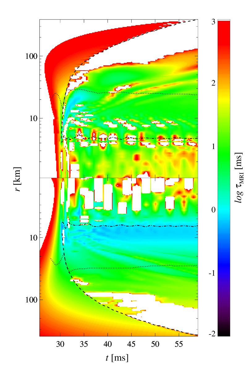
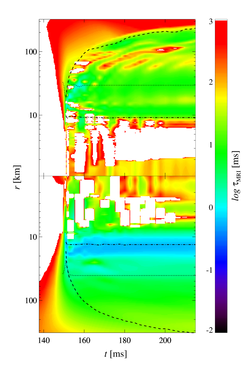
Figure 10: Time evolution of the angular averaged value of the growth time scale $\tau_{\mathrm{MRI}}$ of the fastest growing mode of the MRI for models A1B3G5-D3M0 (left panel) and s20A1B5 (right panel). White regions are stable to the MRI. The top half panels show angular averages of $\tau_{\mathrm{MRI}}$ near the pole ($0<\theta<\pi/6$), while the bottom half panels show these averages near the equator ($\pi/3<\theta<\pi/2$). The shock radius (dashed lines), neutrino sphere radius (dotted line), and radius of shock formation (dash-dotted line) are also displayed.

For a magnetic field distribution with zero mean at large scales, the amplification proceeds from arbitrarily weak fields (Hawley et al. 1996) and saturates irrespective of the initial magnetic field at average values of $P_{\mathrm{mag}}/P_{0}\sim 0.01$, where $P_{0}$ is the initial gas pressure. If a mean magnetic field is present (as in our case), the saturated magnetic field depends on the initial magnetic field strength. In the most favorable case of a vertical magnetic field, the total amplification by the MRI is only about a factor 20 of the original field, this amplification being even smaller in the case of a purely toroidal field (Hawley et al. 1995). On the other hand, Sano et al. (2004) have suggested that for sufficiently weak magnetic fields the saturation level could be independent of the initial field and equal to that in the zero-mean case. If this were confirmed it would mean that, for the weak magnetic field strength present in our magneto-rotational core collapse models ($P_{\mathrm{mag}}/P_{0}\sim 10^{-8}$ in the PNS for progenitors with $B^{*\,0}=10^{10}\mathrm{\ G}$), a magnetic field of $\sim 10^{16}\mathrm{\ G}$ could be reached on time scales of $\tau_{\mathrm{MRI}}$. Such a strong magnetic field would have a significant effect on the dynamics, similar to that observed in numerical simulations with highly magnetized progenitors (Obergaulinger et al. 2006b, a; Shibata et al. 2006). In the opposite case, the MRI would fail to considerably amplify the magnetic field, and for a purely toroidal field the magnetic field should grow only by a factor of about 3 according to Hawley et al. (1995).

The inclusion of more complex physics relevant for the core collapse scenario (like radiation, diffusion, or resistivity) can significantly change the amplification process, since in the nonideal case the reconnection of magnetic field lines seems to be the dominant effect in the saturation process of the MRI. In general, these effects act towards lowering the values of the saturation; for reasons of simplicity we do not consider them in this discussion (see Hawley 2005, and references therein for a detailed review on this topic).

Furthermore, it has to be noted that all local simulations of the MRI have been performed in the context of Keplerian accretion discs, and, hence, some of the underlying physical conditions are not valid in the case of a PNS. For example, the typical sound speed $c_{\mathrm{s}}$ in those simulations is of the order of $10^{-3}$. Only the parametric study performed by Sano et al. (2004) covers a wider range of values of $c_{\mathrm{s}}\sim 10^{-8}\mbox{\,--\,}10^{-2}$ in units of $c$. However, the sound speed in a PNS is higher, $c_{\mathrm{s}}\sim 10^{-1}$. Rotational velocities and profiles are also very different in a disc and a PNS. Therefore, appropriate local simulations of the PNS scenario should eventually be performed in order to confirm the growth of the MRI for a weakly magnetized PNS, and to infer the magnetic field at which the instability saturates.

Our results:

As the MRI involves a backreaction of the magnetic field onto the dynamics, we cannot study this effect in our simulations, as we assume the passive field approximation. Furthermore, even with “active” magnetic fields, both the resolution needed to resolve the MRI length scale ($\sim 10\mathrm{\ m}$) and the requirement for three-dimensional simulations are not affordable with present computers. Therefore, we are limited to analyzing whether our magnetized collapse models are susceptible to developing such an instability according to linear analysis estimates, leaving aside the issue of saturation, whose uncertainties need a deeper analysis which is beyond the scope of this work. In order to estimate how MRI could change our results if it were taken into account properly, we determine the regions where the MRI instability criteria (44) are not satisfied. Inside these regions we calculate the time scale for the fastest growing mode. In Fig. 10 we show the results for the models A1B3G5-D3M0 (left panel) and s20A1B5-D3M0 (right panel). We note that since the onset of the MRI is independent of the magnetic field strength, provided that a poloidal component exists, any composition of D3M0 and T3M0 models has the same instability properties as the D3M0 models.

Our analysis of all computed models shows that during the infall phase the MRI is either not possible or the typical time scales involved are much larger (i.e. $>10\mathrm{\ s}$) than the duration of the collapse itself. Therefore the instability can affect neither the dynamics nor the magnetic field strength in that phase. Around the time of core bounce, the angular velocity gradient is larger and the MRI time scale becomes dynamical. Almost the entire region between the shock formation radius (at $\sim 10\mathrm{\ km}$) and the shock itself is MRI unstable with time scales of the order of $\sim 1\mbox{\,--\,}10\mathrm{\ ms}$. Note that the innermost part of the PNS rotates rigidly, and therefore the MRI unstable region that appears in the inner $2\mathrm{\ km}$ is possibly a numerical artifact caused by the probably unphysical negative entropy gradient mentioned in Sect. 6.2. Some differences appear when comparing microphysical and simplified models.

A general feature of the microphysical models is the post-bounce appearance of a negative entropy gradient (regions with $N^{2}<0$, see Sect. 6.2). This property is much less prominent in the simplified models (except in model A1B3G5). Thus, the presence of a such gradient in the microphysical models enhances the occurence of the MRI behind the shock as compared to the simplified models (see Fig. 10), since in these regions the cause for the instability is mainly the presence of a negative entropy gradient. Around the neutrino sphere the presence or absence of a negative entropy gradient does not affect the onset of the instability since it is caused by the strong negative angular velocity gradient. Therefore, only small differences can be found in the latter region between the simplified and the microphysical models.

As a result of this analysis, for collapse progenitors with a magnetic field smaller than $10^{10}\mathrm{\ G}$ (hence including astrophysically more relevant initial values of $10^{6}\mathrm{\ G}$), we infer that perturbations of the magnetic field are going to grow exponentially on dynamical time scales and will reach saturation in the unstable regions mentioned above. However, the value of the magnetic field at which saturation appears is still unknown, which is a key issue in order to establish the effects of the MRI, if any, on the dynamics. Nevertheless, even if the MRI were unable to considerably amplify the magnetic field, it could still play a major role at late times during the evolution of the PNS, provided other amplification mechanisms were capable to increase the magnetic field to significant larger values (see below). In such a situation the MRI could have an impact on the dynamics by transporting angular momentum outwards and driving the PNS towards rigid rotation.

6.6.3 Dynamo mechanisms

The wind-up process of the magnetic field ($\Omega$-dynamo) discussed before is a mechanism that works by transforming the poloidal magnetic field into a toroidal field and extracting energy from differential rotation. In axisymmetry this process amplifies the magnetic field linearly with time as long as differential rotation exists. If the axisymmetry condition is relaxed, however, a number of instabilities of the toroidal field can transform the toroidal magnetic field back into a poloidal magnetic field. This feedback then “closes” the dynamo process.

The first group of instabilities are those related to convective unstable regions, neutron-finger instabilities (due to a negative composition gradient) and, in general, turbulence. In these cases the $\alpha$-effect is the one which closes the dynamo in the $\alpha\mbox{-}\Omega$-dynamo (Thompson & Duncan 1993). Computations of this effect (Bonanno et al. 2005) suggest that even for a rapidly rotating PNS with a period around $1\mathrm{\ ms}$ (i.e. comparable to the models presented here), the time scale for the growth of the magnetic field is $\sim 1\mathrm{\ s}$. Therefore, this effect is probably not important after core bounce on dynamical time scales. However, for larger time scales (i.e. several seconds), and if the MRI is not efficient enough, this mechanism will most likely amplify the magnetic field, leading to magnetic braking of the PNS within a few seconds.

There are also types of instabilities that can act in stably stratified regions, i.e. regions which are convectively stable. Spruit (1999) has proposed the Tayler instability (Tayler 1973) as a mechanism to close the dynamo. This dynamo has been confirmed in numerical simulations by Braithwaite (2006a, b). The condition for this kink-type instability to grow in the rotating case ($m=1$ mode) is (Spruit 1999)

$$\partial_{\theta}\ln B_{\varphi}^{2}\,\sin\theta\,\cos\theta>0,$$ (47)

which is satisfied almost everywhere inside the star in our simulations. The growth rate of the instability is of the order of the Alfvén time scale,

$$\tau_{\mathrm{T}}=\frac{2\pi}{\Omega_{\mathrm{A}}}\quad(\Omega\ll\Omega_{\mathrm{A}}),\quad\quad\tau_{\mathrm{T}}=\frac{2\pi\Omega}{\Omega_{\mathrm{A}}^{2}}\quad(\Omega\gg\Omega_{\mathrm{A}}),$$ (48)

where $\Omega_{\mathrm{A}}=c_{\mathrm{A}}/R$ and $R$ is the typical size of the region considered. In case this instability appears, it destroys the toroidal magnetic field by transforming it into a poloidal field which feeds back the amplification of the toroidal magnetic field via the $\Omega$-dynamo. Therefore, the dynamo is only effective if the $\Omega$-dynamo is able to generate a toroidal magnetic field faster than the Tayler instability destroys that field, i.e. $\tau_{\mathrm{T}}\gg\tau_{\Omega}$. Saturation is then reached as $\tau_{\mathrm{T}}\approx\tau_{\Omega}$. Note that depending on the system, the saturated magnetic field can be weak enough not to affect the dynamics.

If we consider the typical toroidal magnetic field at bounce to be $10^{13}\mathrm{\ G}$ (as in the T3M0 models) with a typical density in the PNS of $\rho\sim 2\times 10^{14}\mathrm{\ g\ cm}^{-3}$ and a typical size of the inner region of $R\sim 10\mathrm{\ km}$, then the time scale for the growth of the Tayler instability is strongly increased by rotation,

$$\tau_{\mathrm{T}}\approx 3\left(\frac{10^{10}\mathrm{\ G}}{B^{*\,0}}\right)^{2}\left(\frac{R}{10\mathrm{\ km}}\right)^{2}\left(\frac{\Omega_{\mathrm{c}}}{1\mathrm{\ ms}^{-1}}\right)\mathrm{\ hr},$$ (49)

which we obtain from the $\Omega\gg\Omega_{\mathrm{A}}$ limit of Eq. (48).

This means that for a typical progenitor with a toroidal magnetic field of $B^{*\,0}_{\varphi}\sim 10^{10}\mathrm{\ G}$, the instability proposed by Spruit (1999) is going to be very inefficient in amplifying the magnetic field. However, on a longer time scale, when other mechanisms could amplify the magnetic field (e.g. the $\alpha\mbox{-}\Omega$-dynamo), the Tayler instability could also become important.

7 Conclusions

In this paper we have presented numerical simulations of the collapse of rotating magnetized stellar cores in the CFC approximation of general relativity, as well as tests assessing our numerical approach for solving the ideal general relativistic magneto-hydrodynamics (GRMHD) equations.

As initial models we have set up (either fully or nearly) stationary configurations of weakly magnetized stars in general relativity, with either toroidal or poloidal (or both) magnetic field components. We have used the “test” passive field approximation for evolving these initial models, for which the magnetic pressure in all cases considered is several orders of magnitude smaller than the fluid pressure.

We have performed tests to check the accuracy and convergence properties for the GRMHD extension of our code. For magnetic field quantities we have found an order of convergence above 1 in all of the performed tests. These results are consistent with the second-order accuracy (in space and time) of our numerical scheme, reduced to first order only at shocks and local extrema. The errors in all of the cases in which the theoretical solution is known are below 0.1%, except at shocks, which are correctly captured within only few numerical cells thanks to the use of high-resolution shock-capturing schemes.

For the simulations of magnetized core collapse, we have considered cases with magnetic fields which are initially either purely poloidal (series D3M0), purely toroidal (series T3M0), or a combination of both. The D3M0 models are a general relativistic extension of a subset of the cases evolved in fully coupled MHD by Obergaulinger et al. (2006a, b), who used a Newtonian formulation (approximating general relativistic effects to some extent in the latter work). One of our aims has been to compare the dynamics and gravitational waveforms with their results. No qualitative differences have been found in the models studied, while quantitatively the strength of the magnetic field at bounce and after the collapse are consistently smaller in general relativity.

We have also compared simulations of models with improved microphysics (employing a tabulated non-zero temperature equation of state (EOS) and an approximate but effective deleptonization scheme) with the simple (though still widely used) analytic hybrid EOS. The results show that the microphysical models (i) lead to a more complex structure of the poloidal magnetic field due to convective motions surrounding the inner region of the PNS, and (ii) exhibit a wind-up of the magnetic field ($\Omega$-dynamo) that is more efficient than in the simplified models for comparable rotation rates, which is due to the larger compression of the poloidal component during the collapse.

We have found a unified explanation for the magnetic energy of all models, independent of the description of gravity (general relativity or Newtonian) or the EOS, which relates the angular velocity and mass of the PNS with its magnetic energy and the growth rate of the magnetic field due to the $\Omega$-dynamo. This relation shows that higher rotation rates and masses of the PNS lead to stronger magnetic fields. We have shown that it is not possible to mimic the conditions of the microphysical simulations using a simplified EOS. Simplified models with a mass of the homologously collapsing inner core during contraction and a mass of the PNS after bounce similar to the respective masses of the microphysical models (and identical initial rotation profiles) will undergo multiple centrifugal bounces, a behavior that has recently shown to be an artifact of the neglect of microphysics (Dimmelmeier et al. 2007a).

Further differences appear in the appearance of convective motion in the PNS and behind the shock. This convection is more active in microphysical models than in simplified ones. In models with slow rotation, strong convection in the PNS occurs as a transient and disappears within a few ten ms after bounce. Evidently, this transient is an artifact as it does not appear in simulations of similar models with comparable microphysics but using Boltzmann neutrino transport (Müller et al. 2004) instead of our simple advection scheme for the electron fraction after core bounce. In rapidly rotating models convection is not entirely suppressed by rotation but develops and persists on longer time scales, albeit at a lower intensity.

As we have adopted the passive field approximation and the investigated magnetic fields are weak in all phases of the collapse, the waveforms of the gravitational radiation emitted by all our models are practically identical to the corresponding ones in a purely hydrodynamical simulation (Ott et al. 2007a; Dimmelmeier et al. 2007a), with the contribution due to magnetic fields being several orders of magnitude smaller than the total signal amplitude. However, if the MRI could become dominant for the dynamics in the post-bounce phase, in a fully coupled GRMHD simulation we would expect a clear imprint of such an instability on the signal waveform. As expected, for the microphysical models we obtain gravitational wave signals exclusively of Type I, as all other waveform types (in particular the Type II signals associated with multiple centrifugal bounces) are suppressed if more realistic microphysics is taken into account.

For an astrophysically expected strength of the magnetic field (Heger et al. 2005), where the initial toroidal component is much larger than the poloidal one, we have obtained a topology of the magnetic field in the PNS that is purely toroidal due to the radial compression of the initial toroidal component. In this case the time scale for the $\Omega$-dynamo is very long (several hours). For progenitors with stronger poloidal magnetic fields, we have found that a core/shell structure is formed. Inside the core, where nuclear density is exceeded, a mixed configuration of a poloidal and a toroidal magnetic field yields a helicoidal configuration of the field lines. In the surrounding shell (which extends several $10\mathrm{\ km}$) the poloidal magnetic field lines are wound up due to differential rotation ($\Omega$-dynamo), and shortly after core bounce the magnetic field is dominated by the toroidal component. The growth time scale for the toroidal component due to this process is, in the best case scenario, several $100\mathrm{\ ms}$.

We have also estimated the growth times for several other instabilities that could appear if the passive field approximation or the restriction to axisymmetry are removed. Among these the MRI is apparently the fastest growing instability, although it remains unclear if it is going to amplify the magnetic field sufficiently (from the initially weak field values) to affect the dynamics at all. In addition, we have found that the inclusion of microphysics could enhance the MRI, since the regions behind the shock exhibit a negative entropy gradient, resulting in a growth time of $\sim 10\mathrm{\ ms}$ for the MRI. However, the influence of our simplified neutrino treatment or the effects of an alternative microphysical EOS must still be investigated in detail.

In the event that the MRI were unable to sufficiently amplify the magnetic field in the PNS (which is still an open issue), the main amplification mechanism would probably be the $\alpha\mbox{-}\Omega$-dynamo, which can amplify the magnetic field to values where the magnetic energy is in equipartition with the rotational kinetic energy on a time scale of, at least, several seconds. The study of this effect is well beyond the goals of the work presented in this paper, since the required time scales are much longer than those affordable with current numerical magneto-hydrodynamical (MHD) codes. Moreover, the underlying physics necessary to be included (like neutrino transport, diffusion, radiation, and cooling) is far more complex. However, in the light of the results presented here, in which astrophysically expected values for the magnetic field have been adopted, we can speculate about the following scenario. If the MRI is ineffective, after core bounce the magnetic field does not grow significantly strong during one (or maybe several) seconds, and therefore differential rotation generated in the collapse could persist. This “one-second-window” would provide sufficient time for several instabilities to develop in the PNS. Such instabilities are promising sources of gravitational waves.

The restriction to the passive magnetic field approximation in studying magneto-rotational core collapse of weakly magnetized progenitors can be justified if the MRI is indeed inefficient, since none of the other estimated mechanisms seem to be able to amplify the magnetic field significantly on dynamical time scales. Otherwise, an “active” magnetic field approach becomes necessary. However, it has to be stressed that the use of active magnetic fields alone for core collapse simulations will probably not be sufficient to model all the effects amplifying the magnetic field, since the numerical resolution needed to correctly describe them (probably less than $10\mathrm{\ m}$) is not affordable in current numerical simulations. In addition most of the prospectively relevant effects have to be investigated in three dimensions, which makes the computational task even more challenging.

Appendix A Code tests

Here we discuss several tests we have designed in order to check the accuracy of our numerical code when solving the induction equation with the numerical methods described in this paper (see also Cerdá-Durán & Font 2007). The “toroidal test” is set up for assessing the ability of the code to maintain various magnetic field configurations in equilibrium (labelled TTA and TTB) and to correctly compute the amplification of the toroidal magnetic field as it is wound up by a rotating fluid (TTC). On the other hand, the “poloidal test” (PT) is designed to check whether the code can correctly compute the compression of the poloidal magnetic field in a spherical collapse. Finally, the strong spherical explosion test checks that the code is able to handle the presence of radial shocks. We refer the interested reader to Cerdá-Durán & Font (2007) for details on the setup of the toroidal and poloidal tests as well as the diagnostics we use to compute the errors and order of convergence of our numerical schemes.

A.1 Toroidal tests

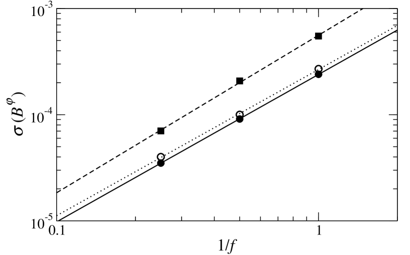
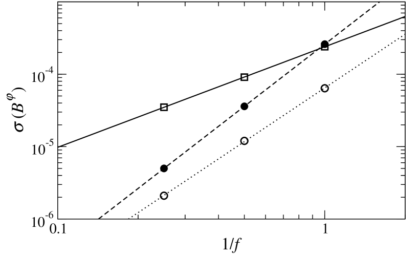
Figure 11: Global error $\sigma$ in the toroidal magnetic field $B^{\varphi}$ after a time evolution of $1\mathrm{\ ms}$ as a function of $1/f$ for a sequence of models with grid resolutions $80\times 10$ ($f=1$), $160\times 20$ ($f=2$) and $320\times 40$ ($f=4$). The top panel shows the error for the TTC test using different reconstruction schemes and the corresponding best fits to a power law: minmod (open circles, dotted line), MC (filled squares, dashed line), and PHM (filled circles, solid line). The bottom panel shows the error and respective fits using the PHM reconstruction for the TTA test (open circles, dotted line), TTB (filled circles, dashed line), and TTC (open squares, solid line).

Fig. 11 shows the global error $\sigma$ in the toroidal magnetic field $B^{\varphi}$ for the three tests TTA, TTB, and TTC against $1/f$ and the corresponding fits to a power law. Here $f$ denotes the factor which specifies the increase in resolution from a coarse reference grid (see Cerdá-Durán & Font 2007, for details). The resulting convergence order of each numerical scheme (minmod, MC, and PHM) as well as the errors for the highest resolution grid can be found in Table 3. Our results show that (i) the order of convergence and the error is almost independent of the cell reconstruction scheme employed, (ii) the order of convergence for the TTC test is smaller than for the TTA and TTB tests, and (iii) the order of convergence for the tests TTA and TTB is $N>2$, and hence higher than the theoretical expectation (which is second order, since it is limited by the order of the time discretization, for which we use a conservative, second order Runge–Kutta scheme).

Table 3: Convergence order $N$ for the tests performed (TTA, TTB, TTC, and PT) and for different reconstruction procedures (minmod, MC, and PHM). The error $\sigma_{320\times 40}$ for the higher resolution grid is also given.

Test	Reconstruction scheme	$N$	$\sigma_{320\times 40}$
TTA	minmod	2.45	$1.2\times 10^{-6}$
TTA	MC	2.16	$2.4\times 10^{-6}$
TTA	PHM	2.46	$2.1\times 10^{-6}$
TTB	minmod	2.64	$7.7\times 10^{-6}$
TTB	MC	2.53	$1.2\times 10^{-5}$
TTC	PHM	2.85	$0.5\times 10^{-6}$
TTC	minmod	1.38	$4.0\times 10^{-5}$
TTC	MC	1.48	$7.0\times 10^{-5}$
TTC	PHM	1.39	$3.5\times 10^{-5}$
PT	minmod	1.41	$8.3\times 10^{-4}$
PT	MC	1.11	$8.6\times 10^{-4}$
PT	PHM	1.17	$8.6\times 10^{-4}$

The numbers reported in Table 3 demonstate that we obtain similar results in all three tests for linear reconstruction schemes (minmod and MC) and for the third order reconstruction scheme (PHM), as the order of the scheme is limited by the second order discretization in time and by the linear interpolation of the cell-centered magnetic fluxes (which is a consequence of using a staggered grid in the flux-CT scheme for the magnetic field). To understand these results we note that in test TTC there is a component of the magnetic field, $B^{*\,\varphi}$, which grows linearly in time, while in tests TTA and TTB no components evolve. Hence, the order of convergence for the latter is higher than for test TTC. This can be explained by investigating the local order of convergence, i.e. the order obtained when computing the error $\sigma_{ij}$ in each numerical cell instead of the global error $\sigma$. The results for test TTA are displayed in Fig. 12 (similar plots can be obtained for the other two cases). At some particular grid zones the order of convergence is larger than two, while at most locations it remains around two.

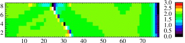
Figure 12: Local order of convergence (color coded) for the TTA test after a total time evolution of $1\mathrm{\ ms}$. White color is used for values $\geq 3.0$. The horizontal and vertical axes represent the number of cells of the reference grid in the radial and angular direction, respectively.

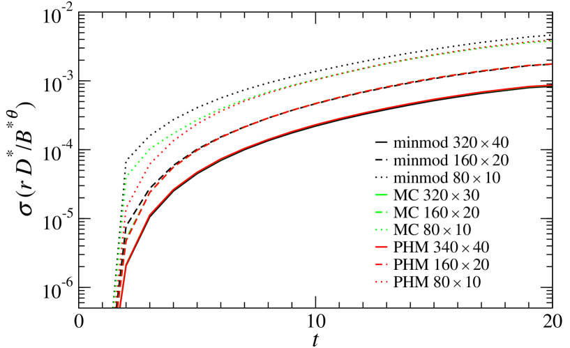
Figure 13: Global error on $r\,D^{*}/B^{*\,\theta}$ for the poloidal test (PT) as a function of time for three different grid resolutions: $80\times 10$, $160\times 20$, and $320\times 40$, and for four different reconstruction schemes (minmod, MC, and PHM).

A.2 Poloidal test

As mentioned before the setup and specifications of the poloidal test are described in detail in Cerdá-Durán & Font (2007). Here we simply focus on showing the comparison and performance of the various numerical schemes employed in our simulations. (Note that in Cerdá-Durán & Font 2007, only the minmod scheme was assessed.) Fig. 13 shows the evolution of the error in the quantity $r\,D^{*}/B^{*\,\theta}$ at the equatorial plane (which is a quantity that should not change with time with respect to a Lagrangian coordinate system) during the spherical collapse of a 4/3-polytrope for different $\{r,\theta\}$ grid resolutions ($80\times 10$, $160\times 20$, and $320\times 40$), equally-spaced in the angular direction and logarithmically spaced in the radial direction. Table 3 gives again numbers for the error and the order of convergence of the various schemes computed at the end of the simulation ($t=20\mathrm{\ ms}$). In all cases the errors are below 1%, even for the coarsest grid, and the order of convergence is higher than 1 (the presence of local extrema in the radial profiles of some hydrodynamical variables explains the reduction of the theoretical order as a built-in feature of total-variation diminishing numerical schemes). Comparisons between the HLL approximate Riemann solver and the KT symmetric scheme yield almost identical results (in agreement with Lucas-Serrano et al. 2004; Shibata & Font 2005; Antón et al. 2006).

A.3 Strong spherical explosion

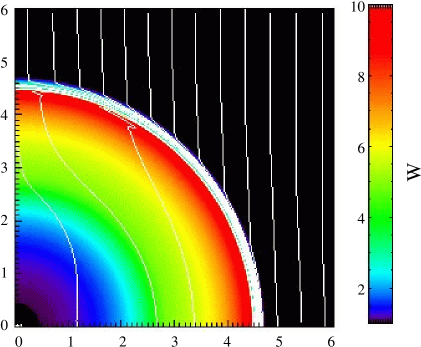
Figure 14: Spherical explosion test at $t=4$. The Lorentz factor $W$ is color coded, and magnetic field lines are overplotted.

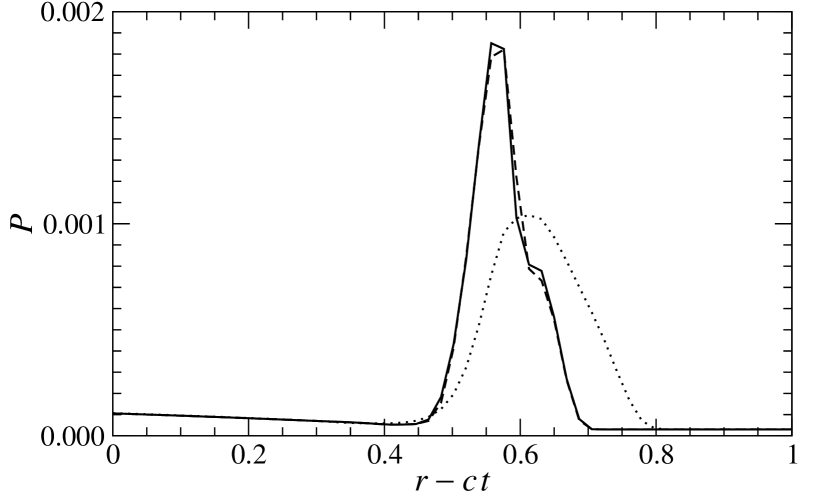
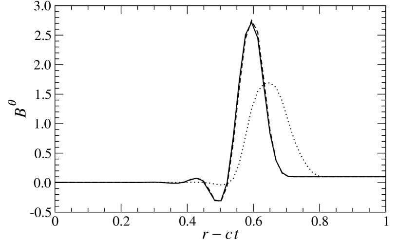
Figure 15: Results for the spherical test explosion at $t=4$. The plots show profiles for the fluid pressure $P$ (top panel) and the magnetic field component $B^{\theta}$ (bottom panel) along the equatorial plane using different reconstruction schemes: minmod (dotted line), MC (dashed line), and PHM (solid line). The grid resolution is $320\times 40$.

Explosions are among the most demanding tests for multi-dimensional codes as they show the ability of numerical schemes to handle shocks. Since the majority of existing MHD codes are written in Cartesian coordinates, the most common test is the cylindrical explosion. For relativistic MHD codes the setup of Komissarov (1999) for this test has been used by other authors (Del Zanna et al. 2003; Leismann et al. 2005) to compare different codes. However, in spherical coordinates it is not possible to impose the symmetries needed for this test. The most natural choice is thus the spherical explosion. Kössl et al. (1990) performed this test in the case of Newtonian MHD. To our knowledge, no spherical explosions tests have been performed in relativistic MHD. Therefore, we have designed such a spherical explosion test in which the initial jump conditions in the variables are the same as for the test by Komissarov (1999). In this way a relativistic shock is formed which does not occur in the Newtonian case of Kössl et al. (1990).

Our test setup consists of an initial explosion zone with $P=1.0$ and $\rho=10^{-2}$ for $r<0.8$, surrounded by an ambient gas with $P=3\times 10^{-5}$ and $\rho=10^{-4}$. The explosion region joins the ambient medium by matching an exponential decline in a transition region region $0.8<r<1.0$. The velocities are initially zero, and the magnetic field is homogeneous and parallel to the symmetry axis. The background spacetime is considered to be flat. The inital data are evolved using an ideal gas EOS with adiabatic index $\gamma=4/3$. We use an evenly spaced grid with a maximum radius of $r=6.0$. We perform the test for three resolutions ($80\times 10$, $160\times 20$, and $320\times 40$) for all reconstruction schemes.

Fig. 14 shows the Lorentz factor $W$ at $t=4.0$. A strong spherical shock has formed, propagating close to the speed of light, and as a consequence the magnetic field lines are compressed in the direction perpendicular to the axis. The results for this test are qualitatively comparable to the weakly magnetized case in Komissarov (1999). Fig. 15 shows radial profiles for $P$ and $B^{\theta}$ along the equatorial plane at the end of the simulation, using various reconstruction schemes. These plots are qualitatively similar to those of the cylindrical explossion (see e.g. Fig. B.4 in Leismann et al. 2005). All numerical schemes exhibit first order convergence with increasing resolution, as is expected to happen at shocks. The MC and PHM schemes yield very similar results, while minmod shows slightly lower values.

Appendix B Estimation of the growth rates of the $\Omega$-dynamo

To compute the characteristic time scales on which the $\Omega$-dynamo mechanism amplifies the magnetic field one has to study how the wind-up proceeds. Let us consider a stationary rotating configuration with no meridional flows, $v^{*\,r}=v^{*\,\theta}=0$ and $v^{*\,\varphi}=\Omega^{*}(r,\theta)\,r\sin\theta$, where $\Omega^{*}(r,\theta)$ stands for the rotation law. Under these conditions and in the passive field approximation, the induction equation can be integrated analytically. The solution shows that the poloidal component of the magnetic field remains constant and the toroidal component grows linearly with time as

$$B^{*\,\varphi}(t)=B^{*\,\varphi}(t=0)+t\,\varpi\,\@vec{B}^{*}\cdot\@vec{\hat{\nabla}}\Omega^{*}.$$ (50)

This equation specifies the toroidal magnetic field at any given time, provided that the poloidal component is constant and the angular velocity profile is fixed. For a time $t\gg B^{*\,0}_{\varphi}/(\varpi\@vec{B}^{*}\cdot\@vec{\hat{\nabla}}\Omega^{*})$, which is $\sim 1\mathrm{\ ms}$ in our simulations, we can use this expression to compute the magnetic energy

$$E_{\mathrm{mag}\,\varphi}\approx\int\mathrm{d}^{3}\mbox{\boldmath$x$}\frac{{B^{*}_{\Omega}}^{2}}{2}\left(\varpi|\@vec{\hat{\nabla}}\Omega^{*}|\right)^{2}\,t^{2},$$ (51)

where $B^{*}_{\Omega}$ is the component of $\@vec{B}^{*}$ parallel to $\@vec{\hat{\nabla}}\Omega^{*}$. The rotation profiles of the final PNS can be approximated in all our models by the rotation law (25) (Villain et al. 2004). In the Newtonian limit (26), which is good enough for this estimate, we can compute an upper limit to the magnetic energy considering the maximum value of $|\varpi\@vec{\hat{\nabla}}\Omega^{*}|_{\mathrm{max}}=\Omega^{*}_{\mathrm{c}}/2$, which yields

$$E_{\mathrm{mag}\,\varphi}\leq E_{\mathrm{mag}\,\Omega}\,\frac{{\Omega^{*}_{\mathrm{c}}}^{2}}{4}\,t^{2}.$$ (52)

Therefore, an estimate for the upper limit of the amplification of the magnetic energy parameter is

$$\beta_{\mathrm{mag}}\approx\beta_{\varphi}\leq\beta_{\Omega}\frac{{\Omega^{*}_{\mathrm{c}}}^{2}}{4}\,t^{2}\leq\beta_{\mathrm{polo}}\frac{{\Omega^{*}_{\mathrm{c}}}^{2}}{4}\,t^{2}=\left(\frac{t}{\tau_{\Omega}}\right)^{2},$$ (53)

where we have defined the time scale for amplification of the magnetic field by the $\Omega$-dynamo as

$$\tau_{\Omega}=\frac{2}{\Omega^{*}_{\mathrm{c}}\sqrt{\beta_{\mathrm{polo}}}}.$$ (54)

This gives us the characteristic time scale in which $\beta_{\mathrm{mag}}$ reaches a value of 1; therefore, the saturation time $t_{\mathrm{sat}}$ should be a fraction of this time. As the $\Omega$-dynamo operates by transforming rotational energy into magnetic energy, the maximum energy can be extracted by the magnetic field is the one that is contained in the differential rotation of the core. In accordance with numerical simulations using strong magnetic fields (Obergaulinger et al. 2006b) we estimate this amount to be 10% of the total rotational energy, i.e. $\beta_{\mathrm{mag}}(t_{\mathrm{sat}})=0.1\,\beta_{\mathrm{rot}}(t_{\mathrm{sat}})$. We also assume that the evolution of the magnetic energy parameter is given by Eq. (53) and that the energy is conserved, i.e. $\beta_{\mathrm{rot}}(t)=\beta_{\mathrm{rot}}(t_{0})-\beta_{\mathrm{mag}}(t)$.