Unstable magnetohydrodynamical continuous spectrum of accretion disks

Abstract

Context. We present a detailed study of localised magnetohydrodynamical (MHD) instabilities occuring in two–dimensional magnetized accretion disks.

Aims. We model axisymmetric MHD disk tori, and solve the equations governing a two–dimensional magnetized accretion disk equilibrium and linear wave modes about this equilibrium. We show the existence of novel MHD instabilities in these two–dimensional equilibria which do not occur in an accretion disk in the cylindrical limit.

Methods. The disk equilibria are numerically computed by the FINESSE code. The stability of accretion disks is investigated analytically as well as numerically. We use the PHOENIX code to compute all the waves and instabilities accessible to the computed disk equilibrium.

Results. We concentrate on strongly magnetized disks and sub–Keplerian rotation in a large part of the disk. These disk equilibria show that the thermal pressure of the disk can only decrease outwards if there is a strong gravitational potential. Our theoretical stability analysis shows that convective continuum instabilities can only appear if the density contours coincide with the poloidal magnetic flux contours. Our numerical results confirm and complement this theoretical analysis. Furthermore, these results show that the influence of gravity can either be stabilizing or destabilizing on this new kind of MHD instability. In the likely case of a non–constant density, the height of the disk should exceed a threshold before this type of instability can play a role.

Conclusions. This localised MHD instability provides an ideal, linear route to MHD turbulence in strongly magnetized accretion disk tori.

1 Introduction

Accretion disks are very common objects in astrophysics. These objects can be found in stellar systems as well as in active galactic nuclei (AGN). In the first case, the disk accretes matter onto a protostar (young stellar object (YSO)), white dwarf, neutron star, or a black hole. The typical size of these disks is a few hundred astronomical units (AU). A massive black hole is the central object in the case of an accretion disk in AGN. Here, the typical size of the disk is a hundred parsecs (pc).

Much research on accretion disk dynamics focuses on occuring accretion processes in an MHD framework. This is done linearly as well as non–linearly. The linear studies aim to understand the drivers of the accretion mechanism. This can be done by looking at waves and instabilities about a disk equilibrium in the cylindrical limit (see e.g. Keppens et al. KCG (2002), Blokland et al. BSKG (2005), van der Swaluw et al. SBK (2005), and references therein). In this limit the disk equilibrium is essentially one–dimensional and one can use a self–similar model like the one of Spruit et al. (SMIS (1987)). When instabilities are found, one must compute the resulting evolution non–linearly to see if these instabilities give rise to turbulence. This turbulence may be the source of an enhanced effective viscosity mechanism which causes an increased transport of angular momentum outwards, as needed for accretion (Shakura & Sunyaev ShSu (1973)). Balbus & Hawley (BaHa (1991)) discussed that the MHD turbulence resulting from the magneto–rotational instability (Velikhov Ve (1959) and Chandrasekhar Ch (1960)) could provide this angular momentum transport.

In the last years, global two or even three–dimensional magnetohydrodynamical (MHD) simulations of accretion disks have been performed (see for example Matsumoto & Shibata MS (1997) and Armitage Am (1998)). In these simulations, the non–linear dynamics is usually interpreted as a direct consequence of the magneto–rotational instability (see for example Hawley et al. HBS (2001)) leading to angular momentum transport outwards. Another possibility for the initial and evolving dynamics is that both the convective and the magneto–rotational instability play an important role in the angular momentum transport (see for example Igumenshchev et al. INA (2003)). In the latter case, these disks are known as convection–dominated accretion flows (CDAF). However,especially those global simulations starting from initial axisymmetric accretion tori (see for example Hawley Haw (2000)) are at best loosely connected to the linear stability studies. A detailed catalogue of the MHD spectrum of such two–dimensional disks is completely lacking. Moreover, the usual identification of the cause of the turbulent dynamics with the linear magneto–rotational or convective instability is mostly based on the extrapolation of the linear stability analysis from a one–dimensional to a two or three–dimensional accretion disk. Such extrapolating ignores the fact that if one performs a detailed MHD stability study of a two–dimensional accretion disk, one may find many new types of instability that all could lead to effective angular momentum transport. A recent example of such new, poloidal flow–driven type of instability is presented by Goedbloed et al. (2004a ), where the Trans–slow Alfvén Continuum (TSAC) mode is shown to occur inside a disk with toroidal and super–slow poloidal flow in the presence of a strong gravitational potential.

This paper has two aims. The first one is to present the equations and the numerical solutions of two–dimensional MHD disk equilibria with toroidal flows, but without poloidal flows. This case is fundamentally different from the previously discussed one of combined poloidal and toroidal flows (Goedbloed et al. 2004a ) because the equilibria are described by quite different flux functions. By considering an axisymmetric equilibrium, we are able to model a thick accretion disk without any further approximations. All the equilibria presented below are computed using the code FINESSE (Beliën et al. BBGHK (2002)). The second aim is to present a detailed stability analysis of these two–dimensional equilibria. The analysis is done theoretically as well as numerically. For the stability computations we have used the recently published spectral code PHOENIX (Blokland et al. BHKG (2006)). To our knowlegde, this kind of analysis for MHD disk equilibria with purely toroidal flow has never been presented in the astrophysical literature until now.

We will present a sample of disk equilibria where the disk plasma typically varies from strongly magnetized up to close to equipartition. Also, the rotational speed of the plasma varies from sub–Keplerian up to Keplerian. The theoretical part of the spectral analysis of these equilibria shows that the convective continuum instabilities may appear inside the disk. These instabilities are part of the continuous branches that exist in the MHD spectrum of the linear eigenmodes of the disk tori and are localised on magnetic flux surfaces. We derive a stability criterion for this instability. This criterion looks similar to the Schwarzschild criterion. However, our criterion governs convective instabilities along the poloidal magnetic field lines while the Schwarzschild criterion applies in the direction perpendicular to the poloidal magnetic field lines. This theoretical analysis has been verified by our numerical stability calculations.

The paper is organised as follows. In Sect. 2, we present the equations which govern a two–dimensional accretion disk equilibrium. In Sect. 3, we recall the essential elements from spectral theory of MHD waves and instabilities, such as the Frieman and Rotenberg formalism (Frieman & Rotenberg FR (1960)), straight field line coordinates and representation. In Sect. 4, these are used to derive the equations for the continuous MHD spectrum and the stability criterion for the convective instability. The numerical codes FINESSE and PHOENIX are discussed in Sect. 5. In Sect. 6, we present our numerical results on the disk equilibria and their stability analysis. Finally, in Sect. 7, we summarise and present our conclusions.

2 Accretion disk equilibrium

We consider an axisymmetric accretion disk. Because of this symmetry, cylindrical coordinates $(R,Z,\varphi)$ are used and the equilibrium quantities only depend on the poloidal coordinates $R$ and $Z$. The disk equilibrium is modeled by the ideal MHD equations,

$$\rho\displaystyle\frac{\partial{\bf{v}}}{\partial t} =-\rho{\bf{v}}\cdot{\bf{\nabla}}{\bf{v}}-{\bf{\nabla}}p+{\bf{j}}\times{\bf{B}}-\rho{\bf{\nabla}}\Phi,$$ (1)

$$\displaystyle\frac{\partial p}{\partial t} =-{\bf{v}}\cdot{\bf{\nabla}}p-\gamma p{\bf{\nabla}}\cdot{\bf{v}},$$ (2)

$$\displaystyle\frac{\partial{\bf{B}}}{\partial t} ={\bf{\nabla}}\times\left({\bf{v}}\times{\bf{B}}\right),$$ (3)

$$\displaystyle\frac{\partial\rho}{\partial t} =-{\bf{\nabla}}\cdot\left(\rho{\bf{v}}\right),$$ (4)

where $\rho$, $p$, ${\bf{v}}$, ${\bf{B}}$, $\Phi$ and $\gamma$ are the density, pressure, velocity, magnetic field, gravitational potential, and the ratio of the specific heats, respectively. The current density ${\bf{j}}={\bf{\nabla}}\times{\bf{B}}$ and the equation ${\bf{\nabla}}\cdot{\bf{B}}=0$ has to be satisfied. Furthermore, the disk equilibrium is assumed to be time-independent. The relation between the density and the thermal pressure is expressed by the ideal gas law: $p=\rho T$. From the equations ${\bf{\nabla}}\cdot{\bf{B}}=0$ and ${\bf{\nabla}}\cdot{\bf{j}}=0$ it follows that the magnetic field and the current density can be written as

$${\bf{B}} =\frac{1}{R}{\bf{e}}_{\varphi}\times{\bf{\nabla}}\psi+B_{\varphi}{\bf{e}}_{\varphi},$$ (5)

$${\bf{j}} =-\frac{1}{R}{\bf{e}}_{\varphi}\times{\bf{\nabla}}I+j_{\varphi}{\bf{e}}_{\varphi},$$ (6)

respectively. Here, $2\pi\psi$ is the poloidal flux and the poloidal stream function $I=RB_{\varphi}$. We restrict ourselves to disk equilibria with purely toroidal flow,

$${\bf{v}}=v_{\varphi}{\bf{e}}_{\varphi}=R\Omega{\bf{e}}_{\varphi}.$$ (7)

In this case, equations (2) and (4) are trivially satisfied. The angular velocity $\Omega$ is related to the electric field,

$${\bf{E}}=-{\bf{v}}\times{\bf{B}}=\Omega{\bf{\nabla}}\psi,$$ (8)

and making use of the induction equation (3) it can be easily shown that $\Omega=\Omega(\psi)$.

Three different projections can be applied on the momentum equation (1). The projections are in the toroidal direction and in the poloidal plane parallel and perpendicular to the poloidal magnetic field lines. From the toroidal projection one can show that the poloidal stream function is a flux function, i.e. $I=I(\psi)$. The projection parallel to the poloidal magnetic field results in two equations,

$$\left.\frac{\partial p}{\partial R}\right|_{\psi=\mathrm{const}} =\rho\left(R\Omega^{2}-\frac{\partial\Phi}{\partial R}\right),$$ (9)

$$\left.\frac{\partial p}{\partial Z}\right|_{\psi=\mathrm{const}} =-\rho\frac{\partial\Phi}{\partial Z},$$

which have to be satisfied simultaneously. From these two equations we conclude that the pressure $p=p(\psi;R,Z)$. The last projection, perpendicular to the poloidal magnetic field, leads to the extended Grad-Shafranov equation,

$$R^{2}{\bf{\nabla}}\cdot\left(\frac{1}{R^{2}}{\bf{\nabla}}\psi\right)=-I\displaystyle\frac{\mathrm{d}I}{\mathrm{d}\psi}-R^{2}\displaystyle\frac{\partial p}{\partial\psi}.$$ (10)

The two equations parallel to the poloidal magnetic field (9) can be solved analytically under the extra assumption that either the temperature $T$, or the density $\rho$, or the entropy $S=p\rho^{-\gamma}$ is a flux function. The assumption that the temperature is a flux function can be justified due to the high thermal conductivity along the magnetic field lines. This is true at least up to the transport time scale, which is long compared to the Alfvén time. The resulting pressure can then be written as

$$p(\psi;R,Z)=p_{0}(\psi)\exp\left[(R^{2}-R_{0}^{2})\Lambda_{T}(\psi)-\frac{\Phi(R,Z)}{T(\psi)}\right],$$ (11)

where $\Lambda_{T}\equiv\Omega^{2}/(2T)$ is a flux function, $p_{0}$ is the pressure for a static pure Grad–Shafranov equilibrium without gravity, and $R_{0}$ is the geometric axis of the accretion disk. The extended Grad-Shafranov equation (10) reduces to

$$\begin{split}R^{2}{\bf{\nabla}}\cdot\left(\frac{1}{R^{2}}{\bf{\nabla}}\psi\right)&=-I\displaystyle\frac{\mathrm{d}I}{\mathrm{d}\psi}-R^{2}\left\{\displaystyle\frac{\mathrm{d}p_{0}}{\mathrm{d}\psi}+p_{0}\left[(R^{2}-R_{0}^{2})\displaystyle\frac{\mathrm{d}\Lambda_{T}}{\mathrm{d}\psi}+\frac{\Phi}{T^{2}}\displaystyle\frac{\mathrm{d}T}{\mathrm{d}\psi}\right]\right\}\\ &\phantom{=-I\displaystyle\frac{\mathrm{d}I}{\mathrm{d}\psi}-R^{2}}\times\exp\left[\left(R^{2}-R_{0}^{2}\right)\Lambda_{T}-\frac{\Phi}{T}\right].\end{split}$$ (12)

Another possibility, on MHD time scales, is to assume that the density is a flux function. In this case, the pressure reads

$$p(\psi;R,Z)=p_{0}(\psi)\left[1+(R^{2}-R_{0}^{2})\Lambda_{\rho}(\psi)-\frac{\Phi(R,Z)}{T_{\rho}(\psi)}\right],$$ (13)

where  the quasi-temperature $T_{\rho}\equiv p_{0}/\rho$ and $\Lambda_{\rho}\equiv\Omega^{2}/(2T_{\rho})$. Under this assumption, the extended Grad-Shafranov equation (10) can be written as

$$\begin{split}R^{2}{\bf{\nabla}}\cdot\left(\frac{1}{R^{2}}{\bf{\nabla}}\psi\right)&=-I\displaystyle\frac{\mathrm{d}I}{\mathrm{d}\psi}-R^{2}\left\{\displaystyle\frac{\mathrm{d}p_{0}}{\mathrm{d}\psi}+p_{0}\left[(R^{2}-R_{0}^{2})\displaystyle\frac{\mathrm{d}\Lambda_{\rho}}{\mathrm{d}\psi}+\frac{\Phi}{T_{\rho}^{2}}\displaystyle\frac{\mathrm{d}T_{\rho}}{\mathrm{d}\psi}\right]\right.\left.\left[1+(R^{2}-R_{0}^{2})\Lambda_{\rho}-\frac{\Phi}{T_{\rho}}\right]^{-1}\right\}\\ &\phantom{=-I\displaystyle\frac{\mathrm{d}I}{\mathrm{d}\psi}-R^{2}}\times\left[1+(R^{2}-R_{0}^{2})\Lambda_{\rho}-\frac{\Phi}{T_{\rho}}\right].\end{split}$$ (14)

The final option is to assume that the entropy $S$ is a flux function. The advantage of this assumption is that it allows for a natural extension to include both toroidal and poloidol flows in the equilibrium, where the entropy has to be a flux function (Zehrfeld et al. ZG (1972); Hameiri Ham (1983)). In this case, the pressure reads

$$p(\psi;R,Z)=p_{0}(\psi)\left\{1+\frac{\gamma-1}{\gamma}\left[(R^{2}-R_{0}^{2})\Lambda_{S}(\psi)-\frac{\Phi(R,Z)}{T_{S}(\psi)}\right]\right\}^{\gamma/(\gamma-1)},$$ (15)

and the extended Grad-Shafranov equation (10) reduces to

$$\begin{split}R^{2}{\bf{\nabla}}\cdot\left(\frac{1}{R^{2}}{\bf{\nabla}}\psi\right)&=-I\displaystyle\frac{\mathrm{d}I}{\mathrm{d}\psi}-R^{2}\left\{\displaystyle\frac{\mathrm{d}p_{0}}{\mathrm{d}\psi}+p_{0}\left[(R^{2}-R_{0}^{2})\displaystyle\frac{\mathrm{d}\Lambda_{S}}{\mathrm{d}\psi}+\frac{\Phi}{T_{S}^{2}}\displaystyle\frac{\mathrm{d}T_{S}}{\mathrm{d}\psi}\right]\right.\left.\left[1+\frac{\gamma-1}{\gamma}\left((R^{2}-R_{0}^{2})\Lambda_{S}-\frac{\Phi}{T_{S}}\right)\right]^{-1}\right\}\\ &\phantom{=-I\displaystyle\frac{\mathrm{d}I}{\mathrm{d}\psi}-R^{2}}\times\left\{1+\frac{\gamma-1}{\gamma}\left[(R^{2}-R_{0}^{2})\Lambda_{S}-\frac{\Phi}{T_{S}}\right]\right\}^{\gamma/(\gamma-1)},\end{split}$$ (16)

where the quasi-temperature $T_{S}\equiv S\rho_{0}^{\gamma-1}$ and $\Lambda_{S}\equiv\Omega^{2}/(2T_{S})$. The extended Grad-Shafranov equation has been used previously by van der Holst et al. (2000b ) for the first two cases without gravity.

The density can be easily derived for all three assumptions by inserting the corresponding equation for the pressure into the momentum equations parallel to the poloidal magnetic field lines (9). The resulting density is

$$\rho(\psi;R,Z)=\rho_{0}(\psi)\times\begin{cases}\left[\left(R^{2}-R_{0}^{2}\right)\Lambda_{T}-\dfrac{\Phi}{T}\right]&\text{for }T=T(\psi)\\ 1&\text{for }\rho=\rho(\psi)\\ \left\{1+\dfrac{\gamma-1}{\gamma}\left[\left(R^{2}-R_{0}^{2}\right)\Lambda_{S}-\dfrac{\Phi}{T_{S}}\right]\right\}^{1/(\gamma-1)}&\text{for }S=S(\psi)\end{cases}.$$ (17)

The flux function $\rho_{0}$ corresponds to the density of a static equilibrium without gravity. All these cases with the inclusion of gravity have been discussed in the appendix to Blokland et al. (BHKG (2006)).

3 Spectral formulation

3.1 Frieman–Rotenberg formalism

For the investigation of stability properties of stationary MHD equilibria, the formalism by Frieman and Rotenberg (FR (1960)) has been used. They derived from the linearised MHD equations, one second order differential equation for the Lagrangian displacement vector field ${\boldsymbol{\xi}}$,

$${\bf{F}}({\boldsymbol{\xi}})-2\rho{\bf{v}}\cdot{\bf{\nabla}}\displaystyle\frac{\partial{\boldsymbol{\xi}}}{\partial t}-\rho\frac{\partial^{2}{\boldsymbol{\xi}}}{\partial t^{2}}=0,$$ (18)

where the force operator ${\bf{F}}({\boldsymbol{\xi}})$ is

$${\bf{F}}({\boldsymbol{\xi}}) ={\bf{F}}_{\mathrm{static}}({\boldsymbol{\xi}})+{\bf{\nabla}}\Phi{\bf{\nabla}}\cdot(\rho{\boldsymbol{\xi}})+{\bf{\nabla}}\cdot\left[\rho{\boldsymbol{\xi}}{\bf{v}}\cdot{\bf{\nabla}}{\bf{v}}-\rho{\bf{v}}{\bf{v}}\cdot{\bf{\nabla}}{\boldsymbol{\xi}}\right].$$ (19)

Here,

$${\bf{F}}_{\mathrm{static}}({\boldsymbol{\xi}}) =-{\bf{\nabla}}\Pi+{\bf{B}}\cdot{\bf{\nabla}}{\bf{Q}}+{\bf{Q}}\cdot{\bf{\nabla}}{\bf{B}}$$ (20)

is the force operator for static equilibria without gravity, which has been derived by Bernstein et al. (BFKK (1958)). Here, the Eulerian perturbation of the total pressure,

$$\Pi =-\gamma p{\bf{\nabla}}\cdot{\boldsymbol{\xi}}-{\boldsymbol{\xi}}\cdot{\bf{\nabla}}p+{\bf{B}}\cdot{\bf{Q}},$$ (21)

and the Eulerian perturbation of the magnetic field,

$${\bf{Q}} ={\bf{\nabla}}\times\left({\boldsymbol{\xi}}\times{\bf{B}}\right).$$ (22)

The time–dependence for the displacement field is assumed to be an exponential one with normal mode frequencies $\omega$, ${\boldsymbol{\xi}}=\hat{{\boldsymbol{\xi}}}\exp(-\mathrm{i}\omega t)$. Using this assumption, the Frieman–Rotenberg equation can be written as

$${\bf{F}}({\boldsymbol{\xi}})+2\mathrm{i}\rho\omega{\bf{v}}\cdot{\bf{\nabla}}{\boldsymbol{\xi}}+\rho\omega^{2}{\boldsymbol{\xi}}=0.$$ (23)

In the derivations below, the toroidal symmetry of the accretion disk equilibrium is exploited. This is done by writing the toroidal dependence of the displacement field as ${\boldsymbol{\xi}}\sim\exp(\mathrm{i}n\varphi)$, where $n$ is the toroidal mode number.

3.2 Straight field line coordinates

The analytical and numerical analysis of MHD waves and instabilities are done in ’straight field line’ coordinates. To convert from cylindrical $(R,Z,\varphi)$ to straight field line coordinates $(x^{1}\equiv\psi,x^{2}\equiv\vartheta,x^{3}\equiv\varphi)$ one needs the metric tensor and the Jacobian associated with the non–orthogonal coordinates in which the equilibrium field lines appear straight. This is standard practice in MHD spectral studies for laboratory tokamak plasmas. The metric elements $g_{ij}$ and the Jacobian $J$ are

$$g^{ij} ={\bf{\nabla}}x^{i}\cdot{\bf{\nabla}}x^{j}, \quad g_{ij} =\frac{\partial{\bf{r}}}{\partial x^{i}}\cdot\frac{\partial{\bf{r}}}{\partial x^{j}}, \quad J =\left({\bf{\nabla}}\psi\times{\bf{\nabla}}\vartheta\cdot{\bf{\nabla}}\varphi\right)^{-1},$$ (24)

respectively. Here, the poloidal angle $\vartheta$ is constructed such that the magnetic field lines are straight in the $(\vartheta,\varphi)$–plane. The slope of these lines is a flux function:

$$\left.\displaystyle\frac{\mathrm{d}\varphi}{\mathrm{d}\vartheta}\right|_{\mathrm{fieldline}}=\frac{{\bf{B}}\cdot{\bf{\nabla}}\varphi}{{\bf{B}}\cdot{\bf{\nabla}}\vartheta}=\frac{IJ}{R^{2}}=q(\psi),$$ (25)

where $q$ is the safety factor. Furthermore, in straight field coordinates the poloidal and toroidal curvature of the magnetic surfaces are

$$\kappa_{\mathrm{p}} =-{\bf{n}}\cdot\left({\bf{t}}\cdot{\bf{\nabla}}{\bf{t}}\right) =\frac{R}{J}\left(\partial_{\psi}-\partial_{\vartheta}\frac{g_{12}}{g_{22}}\right)JB_{\vartheta},$$ (26)

$$\kappa_{\mathrm{t}} =-{\bf{n}}\cdot\left({\bf{e}}_{\varphi}\cdot{\bf{\nabla}}{\bf{e}}_{\varphi}\right) =B_{\vartheta}\left(\partial_{\psi}-\frac{g_{12}}{g_{22}}\partial_{\vartheta}\right)R,$$ (27)

respectively. Here, ${\bf{n}}={\bf{\nabla}}\psi/|{\bf{\nabla}}\psi|$ and ${\bf{t}}={\bf{B}}_{\vartheta}/B_{\vartheta}$, where $B_{\vartheta}$ is the poloidal magnetic field. It is important to realise that the straight field coordinates can only be constructed when the solution $\psi(R,Z)$ has been computed from the extended Grad-Shafranov equation (10).

3.3 Field line projection and representation

On each flux surface the distinction between two wave directions can be made: one parallel and the other one perpendicular to the magnetic field. These directions correspond to the short wavelength limit of slow and Alfvén waves in cylindrical geometry. Hence, it is useful to exploit a projection based on the magnetic surfaces and field lines using the triad of unit vectors,

$${\bf{n}} \equiv\frac{{\bf{\nabla}}\psi}{|{\bf{\nabla}}\psi|}, \quad{\boldsymbol{\pi}} \equiv{\bf{b}}\times{\bf{n}}, \quad{\bf{b}} \equiv\frac{{\bf{B}}}{B}.$$ (28)

Using these unit vectors, the components of the displacement field ${\boldsymbol{\xi}}$ can be written as

$$X \equiv RB_{\vartheta}{\boldsymbol{\xi}}\cdot{\bf{n}}, \quad Y \equiv\mathrm{i}\frac{B}{RB_{\vartheta}}{\boldsymbol{\xi}}\cdot{\boldsymbol{\pi}}, \quad Z \equiv\mathrm{i}\frac{1}{B}{\boldsymbol{\xi}}\cdot{\bf{b}},$$ (29)

and the projected gradient operators become

$$\mathcal{D} \equiv\frac{1}{RB_{\vartheta}}{\bf{n}}\cdot{\bf{\nabla}} =\partial_{\psi}-\frac{g_{12}}{g_{22}}\partial_{\vartheta},$$ (30)

$$\mathcal{G} \equiv-\mathrm{i}RB_{\vartheta}B{\boldsymbol{\pi}}\cdot{\bf{\nabla}} =\frac{-\mathrm{i}I}{J}\partial_{\vartheta}-nB_{\vartheta}^{2},$$ (31)

$$\mathcal{F} \equiv-\mathrm{i}{\bf{B}}\cdot{\bf{\nabla}} =\frac{-\mathrm{i}}{J}\partial_{\vartheta}+\frac{nq}{J}.$$ (32)

The second equality in the expressions for $\mathcal{F}$ and $\mathcal{G}$ only holds when these operators act on a component of the displacement field ${\boldsymbol{\xi}}$.

Using the straight field line coordinates and the projections (29) the Frieman-Rotenberg equation (18) can be written as

$$(\boldsymbol{\mathsf{A}}+\boldsymbol{\mathsf{R}}){\bf{x}}+2\rho\widetilde{\omega}\Omega\boldsymbol{\mathsf{C}}{\bf{x}}-\rho\widetilde{\omega}^{2}\boldsymbol{\mathsf{B}}{\bf{x}} =0, \quad\mathrm{with}\quad{\bf{x}} \equiv\begin{pmatrix}X\\ Y\\ Z\end{pmatrix},$$ (33)

where  $\widetilde{\omega}(\psi)\equiv\omega-n\Omega(\psi)$ is the Doppler shifted eigenfrequency. Here, $\boldsymbol{\mathsf{A}}$ and $\boldsymbol{\mathsf{B}}$ are $3\times 3$ matrix operators which are also present in the case of a static equilibrium without gravity. The matrix operators $\boldsymbol{\mathsf{C}}$ and $\boldsymbol{\mathsf{R}}$ contain the elements due to the toroidal rotation of the plasma and of an external gravitational potential. The matrix elements of $\boldsymbol{\mathsf{A}}$ and $\boldsymbol{\mathsf{B}}$ are

$$\mathrm{A}_{11} \equiv-\mathcal{D}\frac{\gamma p+B^{2}}{J}\mathcal{D}^{\dagger}J+\mathcal{F}\frac{1}{R^{2}B_{\vartheta}^{2}}\mathcal{F}+2\left[\mathcal{D}\left(\frac{B_{\vartheta}\kappa_{\mathrm{p}}}{R}\right)\right]+2\frac{B_{\varphi}}{R}\left[J^{\dagger}\mathcal{D}\left(\frac{1}{J}\frac{B_{\varphi}\kappa_{\mathrm{t}}}{B_{\vartheta}}\right)\right],$$ (34)

$$\mathrm{A}_{12} \equiv-\mathcal{D}\gamma p\mathcal{G}\frac{1}{B^{2}}-\mathcal{D}\mathcal{G}+2\left(\frac{nB_{\vartheta}\kappa_{\mathrm{p}}}{R}+\frac{B_{\varphi}\kappa_{\mathrm{t}}}{B_{\vartheta}}\frac{\mathrm{i}}{J}\partial_{\vartheta}\right),$$

$$\mathrm{A}_{13} \equiv-\mathcal{D}\gamma p\mathcal{F},$$

$$\mathrm{A}_{21} \equiv\frac{1}{B^{2}}\mathcal{G}\frac{\gamma p}{J}\mathcal{D}^{\dagger}J+\mathcal{G}\frac{1}{J}\mathcal{D}^{\dagger}J+2\left(\frac{nB_{\vartheta}\kappa_{\mathrm{p}}}{R}+\frac{\mathrm{i}}{J}\partial_{\vartheta}\frac{B_{\varphi}\kappa_{\mathrm{t}}}{B_{\vartheta}}\right),$$

$$\mathrm{A}_{22} \equiv\frac{1}{B^{2}}\mathcal{G}\gamma p\mathcal{G}\frac{1}{B^{2}}+\mathcal{G}\frac{1}{B^{2}}\mathcal{G}+\mathcal{F}\frac{R^{2}B_{\vartheta}^{2}}{B^{2}}\mathcal{F},$$

$$\mathrm{A}_{23} \equiv\frac{1}{B^{2}}\mathcal{G}\gamma p\mathcal{F},$$

$$\mathrm{A}_{31} \equiv\mathcal{F}\frac{\gamma p}{J}\mathcal{D}^{\dagger}J,$$

$$\mathrm{A}_{32} \equiv\mathcal{F}\gamma p\mathcal{G}\frac{1}{B^{2}},$$

$$\mathrm{A}_{33} \equiv\mathcal{F}\gamma p\mathcal{F},$$

and

$$\mathrm{B}_{11} \equiv\frac{1}{R^{2}B_{\vartheta}^{2}}, \mathrm{B}_{22} \equiv\frac{R^{2}B_{\vartheta}^{2}}{B^{2}}, \mathrm{B}_{33} \equiv B^{2}.$$ (35)

Here, the operators

$$\mathcal{D}^{\dagger} \equiv\mathcal{D}-\left[\partial_{\vartheta}\left(\frac{g_{12}}{g_{22}}\right)\right], {}^{\dagger}\mathcal{D} \equiv\mathcal{D}+\left[\partial_{\vartheta}\left(\frac{g_{12}}{g_{22}}\right)\right],$$ (36)

are related to the normal gradient operator $\mathcal{D}$, which has been introduced by Goedbloed (Go-1997 (1997)) for the spectral analysis of static tokamak equilibria. The square brackets in the expressions (34) for the matrix elements of $\boldsymbol{\mathsf{A}}$ and the gradient operators defined by (36) indicate that the differential operator only acts on the term inside the bracket. This notation is also used in the expressions below. The matrices $\boldsymbol{\mathsf{A}}$ and $\boldsymbol{\mathsf{B}}$ were derived by Goedbloed (Go-1975 (1975), Go-1997 (1997)) for static equilibria.

The matrices $\boldsymbol{\mathsf{R}}$ and $\boldsymbol{\mathsf{C}}$ enter if there is toroidal flow and/or external gravity. The expression for these matrices are

$$\boldsymbol{\mathsf{R}}=\begin{pmatrix}-\rho\left\{\left[J^{\dagger}\mathcal{D}\left(\dfrac{1}{J}\lambda\right)\right]-\dfrac{R\kappa_{\mathrm{t}}}{B_{\vartheta}}\left[\mathcal{D}\Omega^{2}\right]\right\}&\left(\mathrm{i}\mathcal{D}I\mu+\lambda\mathcal{G}\right)\dfrac{\rho}{B^{2}}&\left(\mathrm{i}\mathcal{D}\mu+\lambda\mathcal{F}\right)\rho\\ \dfrac{\rho}{B^{2}}\left(\mathrm{i}I\mu\dfrac{1}{J}\mathcal{D}^{\dagger}J+\mathcal{G}\lambda\right)&-\dfrac{\rho I^{2}}{B^{4}}\left[\dfrac{1}{J}\partial_{\vartheta}\mu\right]&-\rho\left(\dfrac{I}{B^{2}}\left[\dfrac{1}{J}\partial_{\vartheta}\mu\right]-\mathrm{i}n\mu\right)\\ \rho\left(\mathrm{i}\mu\dfrac{1}{J}\mathcal{D}^{\dagger}J+\mathcal{F}\lambda\right)&-\rho\left(\dfrac{I}{B^{2}}\left[\dfrac{1}{J}\partial_{\vartheta}\mu\right]+\mathrm{i}n\mu\right)&-\rho\left[\dfrac{1}{J}\partial_{\vartheta}\mu\right]\end{pmatrix},$$ (37)

$$\boldsymbol{\mathsf{C}}=\begin{pmatrix}0&-\dfrac{R\kappa_{\mathrm{t}}}{B_{\vartheta}}\dfrac{B_{\vartheta}^{2}}{B^{2}}&\dfrac{R\kappa_{\mathrm{t}}}{B_{\vartheta}}\dfrac{I}{R^{2}}\\ -\dfrac{R\kappa_{\mathrm{t}}}{B_{\vartheta}}\dfrac{B_{\vartheta}^{2}}{B^{2}}&0&\mathrm{i}\left[\dfrac{R}{J}\partial_{\vartheta}R\right]\\ \dfrac{R\kappa_{\mathrm{t}}}{B_{\vartheta}}\dfrac{I}{R^{2}}&-\mathrm{i}\left[\dfrac{R}{J}\partial_{\vartheta}R\right]&0\end{pmatrix},$$ (38)

where

$$\mu \equiv\left[\frac{R}{J}\partial_{\vartheta}R\right]\Omega^{2}-\frac{1}{J}\partial_{\vartheta}\Phi=\frac{1}{\rho J}\partial_{\vartheta}p=\frac{1}{\rho}{\bf{B_{\vartheta}}}\cdot{\bf{\nabla}}p,$$ (39)

$$\lambda \equiv\frac{R\kappa_{\mathrm{t}}}{B_{\vartheta}}\Omega^{2}-\mathcal{D}\Phi.$$ (40)

Notice that the term $\mu$ represents the pressure variation on a flux surface. The matrix $\boldsymbol{\mathsf{C}}$ represents the Coriolis effect due to the rotation while the matrix $\boldsymbol{\mathsf{R}}$ contains rotational as well as gravitational effects. The case without an external gravitational potential has been discussed by van der Holst et al. (2000b ).

Two kinds of cylindrical limits can be obtained from the spectral equation (33). The first one is the infinitely slender torus, meaning that the radial position of accretion disk is taken to be at infinity. In that case the matrices $\boldsymbol{\mathsf{R}}$ and $\boldsymbol{\mathsf{C}}$ disappear. This is due to the fact that all equilibrium quantities will be become independent of the angle $\vartheta$, the gravitational potential at infinity is zero, and the toroidal curvature $\kappa_{\mathrm{t}}$ becomes zero. The flow enters only as a Doppler shift, $-n\Omega(\psi)$, in the Doppler shifted eigenfrequency $\widetilde{\omega}(\psi)$.

The other limit is the cylindrical limit of a thin ($|Z|/R\ll 1$) slice of plasma at the equatorial plane of the accretion disk. In this region all equilibrium quantities only depend on the radius $R$, approximately. The matrices $\boldsymbol{\mathsf{R}}$ and $\boldsymbol{\mathsf{C}}$ do not disappear as in the previous limit. Also the toroidal curvature $\kappa_{\mathrm{t}}$ is non–zero but instead the poloidal curvature $\kappa_{\mathrm{p}}=0$. In this case the spectral equation (33) reduces to the matrix equation for a one-dimensional accretion disk presented by Keppens et al. (KCG (2002)).

4 Continuous MHD spectrum

In the previous section, the spectral equation (33) governing all MHD waves and instabilities in axisymmetric accretion disks has been derived. This equation is the starting point to all following MHD spectral computations. In particular, we can derive the equations for the continuous MHD spectrum by considering modes localised on a particular flux surface $\psi=\psi_{0}$. Van der Holst et al. (2000a ) showed that the toroidal flow can drive the continuous spectrum unstable or overstable for non–gravitating plasma tori. Here, we show that the combination of toroidal flow and gravity can also drive the MHD continua overstable.

4.1 General formalism

To derive the equations for the continuous spectrum, the normal derivative $(\partial/\partial\psi)$ of the eigenfunctions is considered to be large compared to the eigenfunctions themselves and the Doppler shifted eigenfrequency $\widetilde{\omega}(\psi)$ is assumed finite. In this case, the first row of the spectral equation (33) can be solved approximately,

$$\frac{1}{J}\mathcal{D}^{\dagger}JX\approx\frac{-\gamma p}{\gamma p+B^{2}}\left(\mathcal{G}\frac{1}{B^{2}}Y+\mathcal{F}Z\right)-\frac{1}{\gamma p+B^{2}}\mathcal{G}Y+\frac{\mathrm{i}\rho\mu}{\gamma p+B^{2}}\left(\frac{I}{B^{2}}Y+Z\right).$$ (41)

Notice, that this solution implies that $\partial X/\partial\psi$, $Y$, and $Z$ are of the same order, but more importantly that $X$ is small compared to $Y$ and $Z$. This means that the continuum modes are mainly tangential to a particular flux surface.

Inserting the expression (41) into the second and third row of the spectral equation (33) results in an eigenvalue problem which is independent of the normal derivative. Hence, the reduced problem becomes non–singular. Exploiting this property, we can write the projected displacement field components $Y$ and $Z$ as follows:

$$Y \approx\delta(\psi-\psi_{0})\eta(\vartheta),$$ (42)

$$Z \approx\delta(\psi-\psi_{0})\zeta(\vartheta),$$

where $\delta(\psi-\psi_{0})$ is the Dirac delta function. Here, $Y$ and $Z$ have been split in an improper ($\psi$–dependence) and proper part ($\vartheta$–dependence). This kind of splitting has been introduced by Goedbloed (Go-1975 (1975)) for static equilibria without gravity. The reduced, non–singular eigenvalue problem becomes

$$\left(\boldsymbol{\mathsf{a}}+\boldsymbol{\mathsf{r}}+2\rho\widetilde{\omega}\Omega\boldsymbol{\mathsf{c}}-\rho\widetilde{\omega}^{2}\boldsymbol{\mathsf{b}}\right)\begin{pmatrix}\eta\\ \zeta\end{pmatrix}=0,$$ (43)

where

$$\boldsymbol{\mathsf{a}}=\begin{pmatrix}\mathcal{F}\dfrac{R^{2}B_{\vartheta}^{2}}{B^{2}}\mathcal{F}+4\dfrac{\gamma p}{\gamma p+B^{2}}\left(RB_{\vartheta}\kappa_{\mathrm{g}}\right)^{2}&-2\mathrm{i}\dfrac{\gamma pB}{\gamma p+B^{2}}\left(RB_{\vartheta}\kappa_{\mathrm{g}}\right)\mathcal{F}\\ 2\mathrm{i}\mathcal{F}\dfrac{\gamma pB}{\gamma p+B^{2}}\left(RB_{\vartheta}\kappa_{\mathrm{g}}\right)&\mathcal{F}\dfrac{\gamma pB^{2}}{\gamma p+B^{2}}\mathcal{F}\end{pmatrix},$$ (44)

$$\boldsymbol{\mathsf{r}}=\begin{pmatrix}-4\dfrac{I}{B^{2}}\dfrac{\rho\mu B}{\gamma p+B^{2}}\left(RB_{\vartheta}\kappa_{\mathrm{g}}\right)+\dfrac{\rho I^{2}}{B^{2}}N_{\mathrm{m,pol}}^{2}&\mathrm{i}I\dfrac{\rho\mu B}{\gamma p+B^{2}}B^{2}\mathcal{F}\dfrac{1}{B^{2}}+\rho IN_{\mathrm{m,pol}}^{2}\\ -\mathrm{i}\dfrac{I}{B^{2}}\mathcal{F}\dfrac{\rho\mu}{\gamma p+B^{2}}B^{2}+\rho IN_{\mathrm{m,pol}}^{2}&-B^{2}\left[\dfrac{1}{JB^{2}}\partial_{\vartheta}\dfrac{\rho\mu}{\gamma p+B^{2}}B^{2}\right]+\rho B^{2}N_{\mathrm{m,pol}}^{2}\end{pmatrix},$$ (45)

$$\boldsymbol{\mathsf{c}}=\begin{pmatrix}0&i\left[\dfrac{R}{J}\partial_{\vartheta}R\right]\\ -i\left[\dfrac{R}{J}\partial_{\vartheta}R\right]&0\end{pmatrix},$$ (46)

$$\boldsymbol{\mathsf{b}}=\begin{pmatrix}\dfrac{R^{2}B_{\vartheta}^{2}}{B^{2}}&0\\ 0&B^{2}\end{pmatrix}.$$ (47)

In these expressions $\kappa_{\mathrm{g}}$ is the geodesic curvature,

$$\kappa_{\mathrm{g}}={\boldsymbol{\kappa}}\cdot{\boldsymbol{\pi}}=\frac{I}{JRB_{\vartheta}B^{2}}\partial_{\vartheta}B.$$ (48)

Here, ${\boldsymbol{\kappa}}={\bf{b}}\cdot{\bf{\nabla}}{\bf{b}}$ is the field line curvature and $N_{\mathrm{m,pol}}^{2}$ is the magnetically modified Brunt-Väisälä frequency projected on a flux surface,

$$N_{\mathrm{m,pol}}^{2} =\frac{\mu}{B^{2}}\left[\frac{1}{J\rho}\partial_{\vartheta}\rho-\frac{\rho\mu}{\gamma p+B^{2}}\right]$$ (49)

$$=\left[\frac{{\bf{B_{\vartheta}}}\cdot{\bf{\nabla}}p}{\rho B}\right]\left[\frac{{\bf{B_{\vartheta}}}}{\rho B}\cdot\left({\bf{\nabla}}\rho-\frac{\rho}{\gamma p+B^{2}}{\bf{\nabla}}p\right)\right].$$

This magnetically modified Brunt-Väisälä frequency is similar as the one presented by van der Holst et al. (2000b ) for tokamaks with purely toroidal flow and as the one for static gravitational plasmas published by Poedts et al. (PHG (1985)) and Beliën et al. (BPG (1997)). Furthermore, notice that the poloidal variation of the pressure presented by the matrix $\boldsymbol{\mathsf{r}}$ shows up in all its matrix elements. This destroys the diagonal dominance of the matrix $\boldsymbol{\mathsf{a}}$, which corresponds to the separation of Alfvén and slow continuum modes. Similar as the matrix $\boldsymbol{\mathsf{C}}$ in spectral equation (33), the matrix $\boldsymbol{\mathsf{c}}$ represents the Coriolis effect.

The non–singular eigenvalue problem (43) is solved for poloidally periodic boundary conditions for the eigenfunctions $\eta$, $\zeta$. Solving this problem for a given toroidal mode number $n$ on each flux surface separately results in a set of discrete eigenvalues. All these discrete sets together map out the continuous spectra. In the MHD formulation with the primitive variables $\rho$, ${\bf{v}}$, $p$, ${\bf{B}}$, an additional entropy continuum $n\Omega$ is found. This Eulerian entropy continuum does not couple to any of the other continua or stable and unstable modes (Goedbloed et al. 2004b ).

4.2 Spectral properties and stability criterion

In this subsection a stability criterium for the continua will be derived. For this derivation we need to construct a Hilbert space with appropriate inner product. The parallel gradient operator $\mathcal{F}$ is a Hermitian operator under the inner product

$$\oint Jv^{*}\left(\mathcal{F}w\right)\mathrm{d}\vartheta=\oint J\left(\mathcal{F}v\right)^{*}w\mathrm{d}\vartheta$$ (50)

for poloidally periodic functions $v$ and $w$. Inspired by this property a Hilbert space can be defined with the inner product

$$\langle{\bf{v}},{\bf{w}}\rangle\equiv\oint{\bf{v}}^{*}\cdot{\bf{w}}J\mathrm{d}\vartheta.$$ (51)

In this Hilbert space, the matrix operators $\boldsymbol{\mathsf{a}}$, $\boldsymbol{\mathsf{b}}$, $\boldsymbol{\mathsf{c}}$, and $\boldsymbol{\mathsf{r}}$ are Hermitian operators. By setting ${\bf{v}}$ and ${\bf{w}}$ equal to the eigenfunctions $(\eta,\zeta)^{\mathrm{T}}$, one can derive a quadratic polynomial for the eigenfrequency $\widetilde{\omega}$ from the spectral equation (43) for the continua.

$$a\widetilde{\omega}^{2}-2b\widetilde{\omega}-c=0.$$ (52)

In this equation, the coefficients are

$$a \equiv\oint\rho\left(\frac{R^{2}B_{\vartheta}^{2}}{B^{2}}|\eta|^{2}+B^{2}|\zeta|^{2}\right)J\mathrm{d}\vartheta,$$ (53)

$$2b \equiv 2i\oint\rho\Omega\left[\frac{R}{J}\partial_{\vartheta}R\right]\left(\eta^{*}\zeta-\eta\zeta^{*}\right)J\mathrm{d}\vartheta,$$ (54)

$$c \equiv\oint\left\{\frac{R^{2}B_{\vartheta}^{2}}{B^{2}}\left|\mathcal{F}\eta\right|^{2}+\frac{\gamma pB^{2}}{\gamma p+B^{2}}\left|\mathcal{F}\zeta+2\mathrm{i}\frac{RB_{\vartheta}\kappa_{\mathrm{g}}}{B}\eta-\mathrm{i}\frac{\rho\mu}{\gamma p}\left(\frac{I}{B^{2}}\eta+\zeta\right)\right|^{2}\right.$$ (55)

$$\phantom{\equiv\oint\left\{\right.}\left.+\rho B^{2}N_{\mathrm{BV,pol}}^{2}\left|\frac{I}{B^{2}}\eta+\zeta\right|^{2}\right\}J\mathrm{d}\vartheta,$$

where $N_{\mathrm{BV,pol}}^{2}$ is the Brunt-Väisälä frequency projected on a flux surface,

$$N_{\mathrm{BV,pol}}^{2} =\frac{\mu}{B^{2}}\left[\frac{1}{J\rho}\partial_{\vartheta}\rho-\frac{\rho\mu}{\gamma p}\right]$$ (56)

$$=\left[\frac{{\bf{B_{\vartheta}}}\cdot{\bf{\nabla}}p}{\rho B}\right]\left[\frac{{\bf{B_{\vartheta}}}}{\rho B}\cdot\left({\bf{\nabla}}\rho-\frac{\rho}{\gamma p}{\bf{\nabla}}p\right)\right]$$

$$=-\left[\frac{{\bf{B_{\vartheta}}}\cdot{\bf{\nabla}}p}{\rho B}\right]\left[\frac{{\bf{B_{\vartheta}}}\cdot{\bf{\nabla}}S}{\gamma BS}\right].$$

Note that the coefficient $a$ is always non zero but, more importantly, that the coefficients $a$, $b$, $c$ are real due to the Hermitian property of the inner product. Solutions of this polynomial are $\widetilde{\omega}=(b\pm\sqrt{b^{2}+ac})/a$. This means that if $b^{2}+ac\geq 0$, the solutions are waves with real frequencies. But if $b^{2}+ac<0$, the solutions contain a damped stable wave and an overstable mode. For the complex solution $\widetilde{\omega}$ one derives its absolute value $|\widetilde{\omega}|=\sqrt{-c/a}$ by taking the linear combination of the polynomial with its conjugate. Furthermore, $\mathrm{Re}(\omega)=n\Omega+b/a$. It can easily be shown that the continuum is stable if $c\geq 0$. The coefficient $c$ is always equal or greater than zero if

$$N_{\mathrm{BV,pol}}^{2}\geq 0$$ (57)

is satisfied everywhere in the plasma. From this stability criterion, we conclude that equilibria with $S=S(\psi)$ and equilibria with $T=T(\psi)$, $\gamma\geq 1$ are always stable. Equilibria where the density is a flux function violate this criterion, which may result in the appearance of damped stable and overstable modes. Notice that the stability criterion (57) is analogous to the Schwarzschild criterion for convective instability. The only important difference is that in the Schwarzschild criterion one deals with normal derivatives while this criterion deals with tangential ones. This has also been noticed by Hellsten & Spies (HeSp (1979)), Hameiri (Ham (1983)), and Poedts et al. (PHG (1985)).

5 Numerical codes

For the stability analysis of axisymmetric accretion tori two numerical codes, the equilibrium code FINESSE (Beliën et al. BBGHK (2002)) and the spectral code PHOENIX (Blokland et al. BHKG (2006)), have been used. In the next two subsections their algorithmic details will be briefly discussed.

5.1 The equilibrium code FINESSE

The FINESSE code developed by Beliën et al. (BBGHK (2002)) can compute a stationary axisymmetric, gravitating MHD equilibrium described by the extended Grad–Shafranov equations (12), (14), or (16) for a given poloidal cross–section and inverse aspect ratio $\epsilon\equiv a/R_{0}$. Here, $a$ and $R_{0}$ are the minor radius of the last closed flux surface and the major radius of the geometric axis, respectively. Fig. 1 shows an example of the geometry of an accretion disk with a circular cross–section as seen in a poloidal plane with the central gravitational object at the origin. The extended Grad–Shafranov equation has been discretized using a finite element method in combination with the standard Galerkin method. The elements used are isoparametric bicubic Hermite ones. These bicubic elements ensure that the computed solution has the desired high accuracy (fourth order) needed for the stability analysis. FINESSE solves the elliptic PDE problem using the Picard iteration scheme. The imposed boundary conditions assume that the fixed boundary represents the last closed flux surface. The same FINESSE code can actually handle the more general case of stationary MHD equilibrium with non–vanishing poloidal flows as well, but here we restrict our discussion to equilibria with purely toroidal flows.

Figure 1: An example of the geometry of an accretion disk with a circular cross-section. Here, $R_{0}$ and $a$ are the major radius of the geometric axis and the radius of the last closed flux surface, respectively

5.2 The spectral code PHOENIX

The spectral code PHOENIX developed by van der Holst (Blokland et al. BHKG (2006)) is used for the stability analysis of a two dimensional accretion disk. PHOENIX can compute the complete MHD spectrum for a given two dimensional equilibrium, toroidal mode number $n$, and a range of poloidal mode numbers $m$. A range of poloidal mode numbers is needed due to the mode coupling caused by allowing for a non–circular cross–section, gravitational stratification, and the toroidal geometry of the accretion disk. PHOENIX does not directly solve the spectral equation (33), but instead employs the linearised version of the full set of MHD Eqs. (1)–(4). These linearised equations are then discretized using a finite element method in the normal $\psi$–direction, a spectral method in the poloidal direction and a standard Galerkin method is used to obtain a linear generalised eigenvalue problem for the eigenfrequencies $\omega$. The elements used in the $\psi$–direction for the perturbed quantities are a combination of quadratic and cubic Hermite elements to prevent the creation of spurious eigenvalues (Rappaz Ra (1977)). This results in a non–Hermitian eigenvalue problem, which is solved using the Jacobi–Davidson method (Sleijpen & van der Vorst SH (1996)). The boundary conditions used for the perturbations are those of a perfect conducting wall. Strictly speaking, these conditions can not be applied to waves and instabilities that appear inside an accretion disk. However, if the wave phenomena are sufficiently localised or not significantly affected by the position of the wall, these boundary conditions have hardly any influence. This is particularly true for the continuous branches of the MHD spectrum on which we concentrate in what follows. These modes are purely localised on a flux surface, and are not affected by the wall. Like FINESSE, PHOENIX can handle poloidal flows as well, but we have exploit it here for equilibria with toroidal flow only.

The continuous spectrum is computed by a less expensive method introduced by Poedts & Schwarz (PS (1993)). In this method, on each individual flux surface the cubic Hermite and the quadratic elements are replaced by $\log(\epsilon)$ and $1/\epsilon$, respectively. Due to this replacement, the singular behaviour of the continuous spectrum has been approximated by the perturbed quantities. This singular behaviour has been described by Goedbloed (Go-1975 (1975)) and Pao (Pa (1975)) for static, axisymmetric and toroidal plasma. Recently, the analogous treatment has been used by Goedbloed et al. (2004a ) for plasmas with toroidal and poloidal flows and gravity. The resulting eigenvalue problem is then a small algebraic problem of a size set by the range in poloidal mode numbers $m$ on each flux surface, and is then solved using a direct QR method and a scan over all flux surfaces. This yields detailed information on all MHD continua.

6 Accretion disks with density as a flux function

We present our numerical results on disk equilibria and stability using the codes described in the previous section. For the equilibrium computations the ratio of the specific heats $\gamma=5/3$ and the gravitational potential is an external Newtonian one, i.e. $\Phi=-GM_{*}/\sqrt{R^{2}+Z^{2}}$, where $G$ and $M_{*}$ are the gravitational constant and the mass of the central object, respectively. Furthermore, we assume that the density is a flux function for all equilibrium computations. From our theoretical analysis above, this is the relevant case which may give rise to damped stable and overstable continuum mode pairs due to the presence of toroidal flow and gravity.

6.1 Thin accretion disk with constant density

As the first case, we take an accretion disk with constant density as also presented by Blokland et al. (BHKG (2006)). The equilibrium is described by the following flux functions:

$$I^{2}(\psi) =A(1-0.0385\psi+0.02\psi^{2}+0.00045\psi^{3}), \rho(\psi) =1,$$ (58)

$$p_{0}(\psi) =AB(1-0.9\psi), \Omega(\psi) =C(1-0.9\psi^{2}),$$

where the values of the coefficients $A$, $B$, and $C$ are given by $112$, $0.01$, and $0.1$. Furthermore, the considered poloidal cross-section is circular and the inverse aspect ratio $\epsilon=0.1$. In these calculations, $GM_{*}=1$ after scaling with respect to a reference density, the vacuum magnetic field, and the minor radius of the accretion disk. Fig. 2 shows the computed two–dimensional pressure and plasma beta $\beta(=2p/B^{2})$ profile. The pressure decreases monotonically outwards due to the fact that the term proportional to the gravitational potential $\Phi$ dominates in the pressure equation (13). In contrast, the plasma beta increases monotonically outwards from $0.63$ at the inner part to $0.76$ at the outer part of the disk. The ratio $v_{\varphi}/v_{\mathrm{Kepler}}=[0.085,1.049]$, where $v_{\mathrm{Kepler}}$ is the Keplerian velocity.

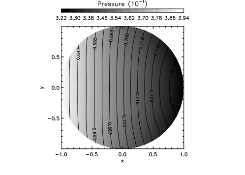
Figure 2: The two–dimensional pressure (gray–scale) and plasma beta $\beta=2p/B^{2}$ (contours) profile for an accretion disk with constant density. The cross–section is circular and the inverse aspect ratio $\epsilon=0.1$. The central object is to the left of the figure.

The computation of the continuous spectrum of this equilibrium is done for toroidal mode number $n=-1$ and poloidal mode numbers $m=[-3,5]$. Fig. 3 shows the sub–spectrum of the MHD continua. The plots clearly indicate the existence of stable and overstable modes in the MHD continua. The plots (a) and (b) show the real and imaginary part of the eigenfrequencies $\omega$ that belong to the continuous spectrum as a function of the radial flux coordinate $s\equiv\sqrt{\psi}$. The frequencies of the continua in the complex plane are shown in the plot (c). It should be noted that it is difficult to label the different branches of the MHD continua by a “dominant” poloidal mode number $m$. This could be done by making use of analytical expressions for an infinitely slender torus ($\epsilon\to 0$), but then the gravity of the central object would be neglected. In our case, these expressions can hardly be used to identify the different branches of the MHD continua, because gravity plays a dominant role in the equilibrium as well as in the spectral analysis. Notice that in plot (a) two branches merge at $s\approx 0.59$, while at the same location the imaginary part of the eigenfrequency starts to become non–zero. Intricate mode couplings thus give rise to the emergence of pairs of overstable and damped stable modes.

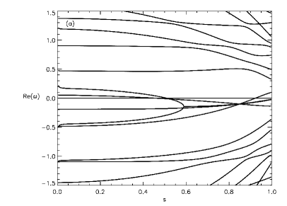
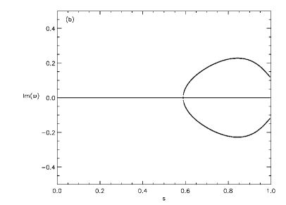
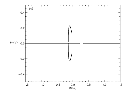
Figure 3: (a) Real, and (b) imaginary parts of the sub–spectrum of the MHD continua as functions of the radial flux coordinate $s\equiv\sqrt{\psi}$ and (c) represented in the complex plane for toroidal mode number $n=-1$ and poloidal mode numbers $m=[-3,5]$. The corresponding disk equilibrium shown in Fig. 2 has a constant density distribution.

Next, we investigate the influence of the external gravitational potential on the overstable modes presented in the previous figure. This is done by varying the mass of the central object $GM_{*}$. The result is shown in Fig. 4, where the most overstable mode of the MHD continua is plotted as function of the gravitational potential on the magnetic axis $R_{\mathrm{M}}$. Notice that each point in this plot corresponds to a different equilibrium calculated with FINESSE. PHOENIX is used to analyse the stability of the computed equilibrium. The gravitational potential is stabilizing from 0 to -0.01 and destabilizing from -0.01 to lower values. The zero value corresponds to a toroidally rotating, non-gravitating “tokamak” plasma. Its instability is in agreement with the results by van der Holst et al. (2000a ). Fig. 5 shows the projected Brunt-Väisälä frequency for the points (a), (b), and (c) indicated in Fig. 4. Plot (a) shows that the minimum value of this frequency is reached inside the plasma, while plot (c) shows that this value is reached at the edge of the accretion disk. Point (b) is the transition from the minimum value inside to the edge of the disk as seen in plot (b).

Figure 4: The growth rate of the most unstable continuum mode as a function of the value of gravitational potential on the magnetic axis $R_{\mathrm{M}}$. The gravitational potential is scaled with respect to the Alfvén speed on the magnetic axis.

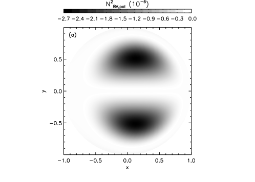
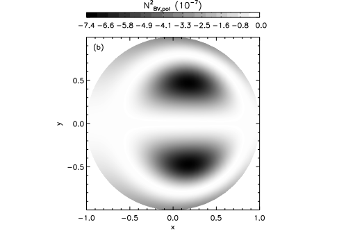
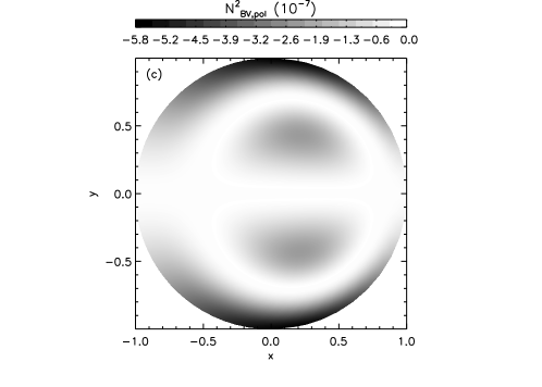
Figure 5: The Brunt-Väisälä frequency projected on a flux surface for the points (a), (b), and (c) shown in Fig. 4 shown as a contour plot in a poloidal cross–section.

6.2 Thin accretion disks with non–constant density

To model a more realistic accretion disk equilibrium, we allow a density gradient across the poloidal magnetic surfaces. All other flux functions are kept as in the previous case, i.e.

$$I^{2}(\psi) =A(1-0.0385\psi+0.02\psi^{2}+0.00045\psi^{3}), \rho(\psi) =1-0.4\psi,$$ (59)

$$p_{0}(\psi) =AB(1-0.9\psi), \Omega(\psi) =C(1-0.9\psi^{2}),$$

where the coefficients $A$, $B$, $C$ are given by $91.5$, $0.01$, and $0.1$. Also in this case, the poloidal cross–section is circular, the inverse aspect ratio $\epsilon=0.1$, and the scaled mass of the central object is $GM_{*}=1$. The two–dimensional pressure and plasma beta profile are shown in Fig. 6. This profile shows that the pressure reaches its maximum within the disk, instead of at the inner boundary of the disk, as in the case of a constant density. This difference can be explained as follows. Here, also the term $p_{0}\Phi(R,Z)/T_{\rho}=\rho\Phi(R,Z)$ dominates in the pressure equation (13), but, due to the small inverse aspect ratio, the variation in the gravitational potential is small compared to the one in the density. This implies that the density, which is a flux function, mainly determines the shape of the dominant term in the Eq. (13). The temperature (not shown) decreases monotonically outwards. The range of plasma beta $\beta=[0.082,0.158]$ and its maximum value is reached within the accretion disk. These low values for the plasma beta imply that the disk is strongly magnetized. Furthermore, the range of the ratio $v_{\varphi}/v_{\mathrm{Kepler}}=[0.085,1.044]$.

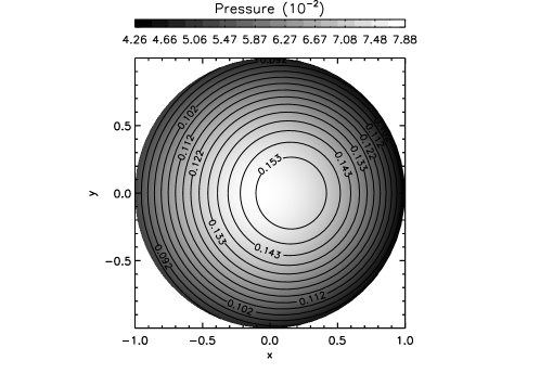
Figure 6: The pressure (gray–scale) and plasma beta $\beta=2p/B^{2}$ (contours) distribution in a poloidal cross–section for an accretion disk with density $\rho\propto(1-0.4\psi)$ and an inverse aspect ratio $\epsilon=0.1$.

For this case, the continuous spectrum has been computed for toroidal mode number $n=1$ and poloidal mode numbers $m=[-3,5]$. The results are shown in Fig. 7, which contains two plots. In the left one, the real part of the eigenvalues is plotted against the “radial” coordinate $s\equiv\sqrt{\psi}$, while the right one shows the eigenvalues in the complex plane. For this case, there are neither purely exponential unstable or overstable modes. Due to the presence of toroidal flow, gravity and a non–constant density, it is possible to create new or wider gaps between the different MHD continuum branches, with avoided crossings as a result of poloidal mode couplings. This has been shown by van der Holst et al. (2000b ) for tokamak equilibria with toroidal flow. In these gaps, there may exist global modes similar to the Toroidal Flow–induced Alfvén Eigenmode (TFAE) for tokamaks found by van der Holst et al. (2000a ) or to the Stratification–induced Alfvén Eigenmode (SAE) for coronal flux tubes found by Beliën et al. (BPG-L (1996)). We will investigate this possibility for novel global modes in accretion disk context in future work.

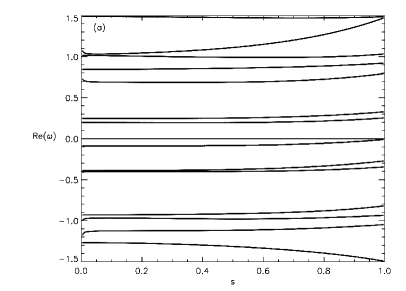
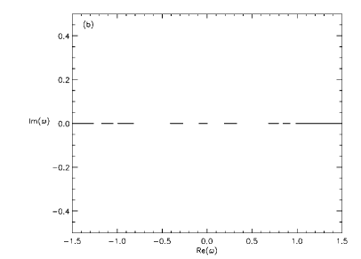
Figure 7: For the accretion disk equilibrium shown in Fig. 6, (a) the real parts of the sub–spectrum of MHD continua as function of the radial flux coordinate $s\equiv\sqrt{\psi}$ and (b) sub–spectrum of the MHD continua in the complex plane are shown for toroidal mode number $n=-1$ and poloidal mode numbers $m=[-3,5]$. For these mode numbers, no unstable or overstable modes are found.

6.3 Thick accretion disk

Next, we increase the inverse aspect ratio $\epsilon$ from 0.1 to 0.5, while keeping all other quantities the same. Again, the poloidal cross–section is chosen circular. The resulting pressure profile is presented in Fig. 8. Here, The pressure decreases monotonically outward, similar to the equilibrium with constant density. Again, the term $\rho\Phi(R,Z)$ dominates in the pressure equation (13). The inverse aspect ratio is now not small so that both the gravitational potential and the density determines the shape of the pressure profile. Also in this case, the temperature decreases in the outward direction. The plasma beta $\beta$ of this accretion disk ranges from 0.237 up to 0.970 and reaches its maximum within the disk. The deviation from a Keplerian disk is expressed by the ratio $v_{\phi}/v_{\mathrm{Kepler}}=[0.007,0.282]$. Thus the disk completely rotates sub-Keplerian.

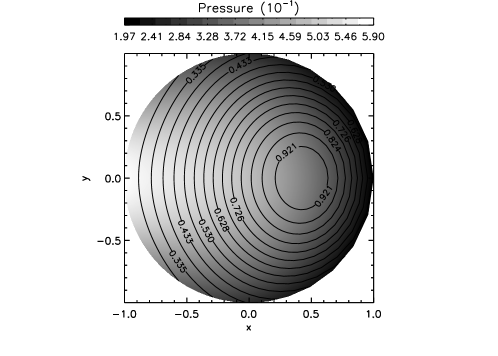
Figure 8: The pressure (gray–scale) and plasma beta $\beta=2p/B^{2}$ (contours) for a thick accretion disk with density $\rho\propto(1-0.4\psi)$ and an inverse aspect ratio $\epsilon=0.5$.

For this equilibrium, the continuous MHD spectrum is computed, again for toroidal mode number $n=-1$ and poloidal mode numbers $m=[-3,5]$. A part of the spectra is plotted in Fig. 9. Plot (a) shows the real part of the continuous MHD spectrum, while plot (c) shows the imaginary part as a function of the radial flux coordinate $s\equiv\sqrt{\psi}$. Plot (c) contains the eigenfrequencies plotted in the complex plane. This shows the existence of overstable modes in a thick accretion disk due to the presence of toroidal flow and gravity. If one carefully examines the plot (a) one sees that one of the continuum branches splits in two at $s\approx 0.87$, where the imaginary part becomes zero and at $s\approx 0.91$ that these two continuum branches merge again, whereas the imaginary part becomes non–zero.

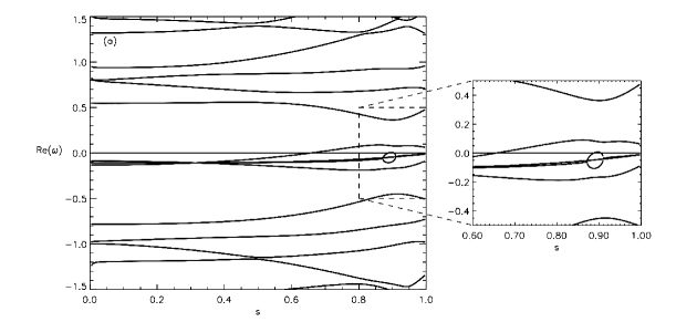
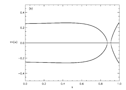
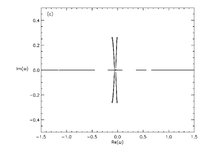
Figure 9: For the thick disk equilibrium shown in Fig. 8, (a) the real and (b) imaginary parts of the sub–spectrum of the MHD continua as a function of the radial flux coordinate $s\equiv\sqrt{\psi}$ and (c) sub–spectrum of the MHD continua in the complex plane are shown for toroidal mode number $n=-1$ and poloidal mode numbers $m=[-3,5]$.

6.4 Maximum growth rate of the MHD continua of thin and thick accretion disks

The last two cases only differ by the value of the inverse aspect ratio $\epsilon$. We have systematically investigated the influence of this ratio on the existence of overstable modes by varying its value, while keeping all other equilibria quantities constant. In this parametric study, we essentially move the disk torus radially inwards while keeping the radius of the last closed flux surface $a$ constant. We then gradually evolve from the equilibrium shown in Fig. 6 ($\epsilon=0.1$) to the one shown in Fig. 8 ($\epsilon=0.5$). The growth rate of the most overstable continuum mode is plotted as a function of the inverse aspect ratio $\epsilon$ in Fig. 10. Each point of the figure represents an equilibrium computed by FINESSE, from which the MHD continua is computed by PHOENIX. In this figure, one can clearly see that no overstable modes are present in these disks for $\epsilon=[0.10,0.24]$. From $\epsilon=0.24$ up to $0.32$, there is a strong increase of the growth rate of the most overstable mode, while from $\epsilon=0.32$ up to at least $0.50$ the growth rate remains approximately the same.

Figure 10: Growth rate of the most overstable continuum mode as a function of the inverse aspect ratio $\epsilon=a/R_{0}$.

7 Conclusions

We have presented the equations describing an axisymmetric MHD accretion disk equilibrium and used FINESSE to find numerical solutions. We have considered thin as well as thick disks with a plasma beta of the order $0.1$ where the largest part of the disk rotates sub–Keplerian. The numerical solutions show that the pressure profile can only decrease in the outward direction if the gravitational potential dominates in the pressure equation (13).

The stability of the disk equilibria have been analysed theoretically as well as numerically. From theory, a stability criterion has been derived which closely resembles the Schwarzschild criterion. It is shown that in a disk where the density is a flux function, the MHD continua can turn overstable due to the presence of toroidal rotation and gravity. This instability is not possible for disks where the temperature or the entropy is a flux function. The numerical results support our theoretical conclusion. The effect of the gravity on the overstable modes can either be stabilizing or destabilizing. In the case of non–constant density the inverse aspect ratio $\epsilon$ has been varied. This study shows that the continua turn overstable if the inverse aspect ratio is larger than a certain critical value, approximately 0.24. These localised instabilities will lead to small–scale, turbulent dynamics when the equilibria are used in initial conditions for non–linear simulations. This dynamics is unrelated the usual magneto–rotational instability. Indeed, these instabilities, as well as the poloidal flow driven unstable continuum modes investigated by Goedbloed et al. 2004a , provide a new route to MHD turbulence in accretion disks. Furthermore, due to the presence of gravity, it is possible to widen or create new gaps in the MHD continua. It is possible to show this theoretically by expanding the eigenfunctions in poloidal harmonics. In these gaps new types of global ideal MHD eigenmodes can exist. The investigation of these global eigenmodes is left for future work.

- (1) Armitage, P. 1998, ApJ, 501, L189
- (2) Balbus, S. A., & Hawley, F. H. 1991, ApJ, 376, 214
- (3) Beliën, A. J. C., Botchev, M. A., Goedbloed, J. P., van der Holst, B., & Keppens R. 2002, J. Comp. Physics, 182, 91
- (4) Beliën, A. J. C., Poedts, S., & Goedbloed, J. P. 1996, Phys. Rev. Lett., 76, 567
- (5) Beliën, A. J. C., Poedts, S., & Goedbloed, J. P. 1997, A&A, 332, 995
- (6) Bernstein, I. B., Frieman, E. A., Kruskal, M. D., & Kulsrud, R. M. 1958, Proc. Roy. Soc. of London, A, 17
- (7) Blokland, J. W. S., van der Swaluw, E., Keppens, R., & Goedbloed, J. P. 2005, A&A, 444, 337
- (8) Blokland, J. W. S., van der Holst, B., Keppens, R., & Goedbloed, J. P. 2006, J. Comp. Physics, submitted
- (9) Chandrasekhar, S. 1960, Proc. Nat. Acad. Sci USA, 46, 53 (Oxford University Press)
- (10) Frieman, E., & Rotenberg, M. 1960, Rev. Mod. Phys., 32, 898
- (11) Goedbloed, J. P. 1975, Phys. Fluids, 18, 1258
- (12) Goedbloed, J. P. 1997, Trans. Fusion Technol., 33, 115
- (13) Goedbloed, J. P., Beliën, A. J. C., van der Holst, B., & Keppens, R. 2004, Phys. Plasmas, 11, 28
- (14) Goedbloed, J. P., Beliën, A. J. C., van der Holst, B., & Keppens, R. 2004, Phys. Plasmas, 11, 4332
- (15) Hameiri, E. 1983, Phys. Fluids, 26, 30
- (16) Hawley, J. F. 2000, ApJ, 528, 462
- (17) Hawley, J. F., Balbus, S. A., & Stone, J. M. 2001, ApJ, 554, L49
- (18) Hellsten, T. A. K., & Spies, G. O. 1979, Phys. Fluids, 22, 743
- (19) van der Holst, B., Beliën, A. J. C., & Goedbloed, J. P. 2000, Phys. Rev. Lett.., 84, 2865
- (20) van der Holst, B., Beliën, A. J. C., & Goedbloed, J. P. 2000, Phys. Plasmas, 7, 4208
- (21) Igumenshchev, I. V., Narayan, R., & Abramowicz, M. A. 2003, ApJ, 592, 1042
- (22) Keppens, R., Casse, F., & Goedbloed, J. P. 2002 ApJ, 569, L121
- (23) Matsumoto, R., & Shibata, K. 1997, in IAU Colloq. 163, Accretion Phenomena and Related Outflows, ed. D. Wickramsinghe, G. Bicknell & L. Ferrario (ASP Conf. Ser. 121; San Francisco: ASP), 443
- (24) Pao, Y. P. 1975, Nucl. Fusion, 15, 631
- (25) Poedts, S., Hermans, D., & Goossens, M. 1985, A&A, 151, 16
- (26) Poedts, S. & Schwarz, E. 1993, J. Comp. Phys., 105, 165
- (27) Rappaz, J. 1977, Numer. Math., 28, 15
- (28) Shakura, N. I., & Sunyaev, R. A. 1973, A&A, 24, 337
- (29) Sleijpen, G. L. G. & van der Vorst, H. A. 1996, SIAM J. Matrix Anal. Appl., 17, 401
- (30) Spruit, H. C., Matsuda, T., Inoue, M., & Sawada, K. 1987, MNRAS, 229, 517
- (31) van der Swaluw, E., Blokland, J. W. S., & Keppens, R. 2005, A&A, 444, 347
- (32) Velikhov, E. P. 1959, Sov. Phys. JETP, 36(9), 995
- (33) Zehrfeld, H. P. & Green, B. J. 1972, Nucl. Fusion, 12, 569