Testing the predicted mass-loss bi-stability jump at radio wavelengths

Abstract

Context. Massive stars play a dominant role in the Universe, but one of the main drivers for their evolution, their mass loss, remains poorly understood.

Aims. In this study, we test the theoretically predicted mass-loss behaviour as a function of stellar effective temperature across the so-called ‘bi-stability’ jump.

Methods. We observe OB supergiants in the spectral range O8-B3 at radio wavelengths to measure their thermal radio flux densities, and complement these measurements with data from the literature. We derive the radio mass-loss rates and wind efficiencies, and compare our results with H$\alpha$ mass-loss rates and predictions based on radiation-driven wind models.

Results. The wind efficiency shows the possible presence of a local maximum around an effective temperature of 21 000 K – in qualitative agreement with predictions. Furthermore, we find that the absolute values of the radio mass-loss rates show good agreement with empirical H$\alpha$ rates derived assuming homogeneous winds – for the spectral range under consideration. However, the empirical mass-loss rates are larger (by a factor of a few) than the predicted rates from radiation-driven wind theory for objects above the bi-stability jump (BSJ) temperature, whilst they are smaller (by a factor of a few) for stars below the BSJ temperature. The reason for these discrepancies remains as yet unresolved. A new wind momenta-luminosity relation (WLR) for O8-B0 stars has been derived using the radio observations. The validity of the WLR as a function of the fitting parameter related to the force multiplier $\alpha_{\rm eff}$ (Kudritzki & Puls 2000) is discussed.

Conclusions. Our most interesting finding is that the qualitative behaviour of the empirical wind efficiencies with effective temperature is in line with the predicted behaviour, and this presents the first hint of empirical evidence for the predicted $mass$-$loss$ bi-stability jump. However, a larger sample of stars around the BSJ needs to be observed to confirm this finding.

1 Introduction

Massive stars are the main drivers for the evolution of galaxies: they are the prime contributors to the energy and momentum input into the interstellar medium through stellar winds and supernovae, they generate the bulk of ionising radiation, and they are important sources for the chemical enrichment of carbon, oxygen and nitrogen in the Universe. Their very evolution through subsequent stages (OB –$>$ LBV –$>$ WR –$>$ SN) is believed to be driven by mass loss (e.g. Chiosi & Maeder 1986). Heger et al. (2003) have recently reviewed the way in which massive stars end their lives and they find that the type of remnant that is left – neutron star, black hole, or no remnant at all – is primarily dependent on the amount of mass lost via stellar winds.

The physical mechanism for these winds of massive OB stars has long been identified to be that of radiation pressure on millions of spectral lines (Lucy & Solomon 1970; Castor Abbott & Klein 1975: hereafter CAK). These radiation-driven wind models predict the mass-loss rates $\dot{M}$ of O stars to depend strongly on the stellar luminosity, and the terminal flow velocity ($v_{\infty}$) to be proportional to the escape velocity ($v_{\rm esc}$), reaching wind velocities of thousands of km s^-1. Over the last decades, the theory has proven to be very successful in explaining the overall mass-loss properties of O stars, with $\dot{M}$ of O stars up to 10^-5 M_⊙ yr^-1 and a clear correlation between the wind terminal and the escape velocity: ($v_{\infty}/v_{\rm esc}$) $\simeq$ 2.6 (Kudritzki & Puls 2000).

Nevertheless, there are many open issues in the field of massive star evolution and their winds – even during the “best understood” O & B evolutionary phases. One of them is that of wind clumping (e.g. Eversberg et al. 1998). Many modern evolution models (Maeder & Meynet 2003, Limongi & Cioffi 2006, Eldridge & Vink 2006) use OB mass-loss rates from smooth wind Monte Carlo mass-loss predictions of Vink et al. (2000a, 2000b). However, the sizes of these mass-loss rates have recently been questioned by a number of ultraviolet (UV) studies, and downward revisions by factors of five to ten have been suggested (Bouret et al. 2003, Fullerton et al. 2006). There are theoretical and observational indications (e.g. Evans et al. 2004) that the winds of OB stars are clumped, but what remains uncertain is by what factor the mass-loss rates could be over-predicted; is it as dramatic (i.e. factors $\sim$ 10) as has been suggested by the UV studies, or is the clumping factor relatively small (a factor of $\sim$ two)?. It is relevant to note that a modest amount of wind clumping is actually required to match the Vink et al. (2000a, 2001) mass-loss predictions. If the clumping factor ($f$) is only $\sim$ 5 - the corresponding mass-loss rates are a factor $\sqrt{5}$ lower- (Repolust et al. 2004, Mokiem et al. 2007), massive star evolution is not anticipated to be dramatically affected by clumping. For a recent discussion on wind clumping from optical studies, we refer to Puls et al. (2006), and Davies et al. (2007).

Another topical issue is that of the “bi-stability jump” (BSJ): an empirical drop in the ratio ($v_{\infty}/v_{\rm esc}$) from 2.6 to 1.3 around temperatures of about 21 000 K (Lamers et al. 1995). Theoretically, the wind characteristics as a function of stellar spectral type are best described in terms of the wind efficiency number: $\eta=(\dot{M}v_{\infty})/({L_{*}/c})$, a measure for how much momentum from the photons is transferred to the ions of the outflowing wind. Vink et al. (2000a) computed a large grid of wind models as a function of effective temperature and presented the following overall behaviour of the mass-loss rate as a function of decreasing temperature (Fig. 1).

Over the temperature range between 50 000 K down to 27 500 K, the mass-loss rates drop rapidly. The reason is that of a growing mismatch between the wavelengths of the maximum opacity in the UV and the flux maximum, which progressively moves from extreme UV (Ly continuum) to far UV, from early O to early B stars. The behaviour is however reversed around the BSJ, where $\eta$ is now predicted to increase by a factor of 2-3 to a local maximum when Fe iv recombines to the more efficient Fe iii configuration (Vink et al. 1999, Vink 2000). Below the BSJ, the first effect returns, and $\eta$ is again predicted to decrease with temperature.

Figure 1: The predicted wind efficiency number: $\eta=(\dot{M}v_{\infty})/({L_{*}/c})$ as a function of effective temperature (from Vink et al. 2000a). Note the presence of a local maximum at the position of the bi-stability jump around $T_{\rm eff}=21\leavevmode\nobreak\ 000$K.

For B supergiants, Vink et al. (2000a) reported significant discrepancies between empirical and predicted mass-loss rates. Recent studies involving H$\alpha$ (Trundle & Lennon 2005, Crowther et al. 2006) and UV analyses (Prinja et al. 2005) have reconfirmed these findings. However, discrepancies between empirical UV rates and radiation-driven wind models have now also been reported for O stars (see Fullerton et al. 2006). It is currently unclear whether the reported discrepancies for B supergiants are due to the assumption of smooth winds (and the neglect of wind clumping) in the radiation-driven wind model for all spectral types, or instead that they are somehow related to the physics of the BSJ.

1.1 The bi-stability jump

The bi-stability jump was first discussed by Pauldrach & Puls (1990) in the context of their model calculations of an individual star, the Luminous Blue Variable (LBV) P Cygni. The first empirical work on the BSJ for a sample of stars was that by Lamers et al. (1995), who found a discontinuity in the ratio ($v_{\infty}/v_{\rm esc}$) at spectral type B1 ($T_{\rm eff}$ $\sim$ 21 000 K). For the earlier-type stars the ratio is $\simeq$ 2.6, but for the lower temperatures it drops to $\simeq$ 1.3. They also discussed the possible existence of a second BSJ at spectral type A0. We note that Crowther et al. (2006) performed a sophisticated analysis using line-blanketed model atmospheres (of Hillier & Miller 1998) of the temperatures of objects around the B1 BSJ and concluded the empirical BSJ in wind velocity represents a more gradual decrease than suggested by the step function of Lamers et al. (1995).

On the theoretical front, Vink et al. (1999) studied the nature of the winds around the BSJ and found a gradual change in wind properties, while they attributed the origin of the BSJ to a gradual change in the ionization of the Fe lines that drive the wind. For a range of stellar parameters and adopted velocity laws, Vink et al. (1999, 2000a) found an increase in the wind efficiency $\eta$ by a factor 2-3 independent of the assumed terminal velocity. When accounting for the empirical drop in terminal velocity, they found a jump in the mass-loss rate by a factor of five – for stars at the same luminosity. They argued that the jump in mass loss is accompanied by a decrease of the ratio ($v_{\infty}/v_{\rm esc}$), which is the observed bi-stability jump in terminal velocity. Using self-consistent models they obtained ratios within 10 percent of the observed values around the jump (Vink et al. 1999, 2000b; Vink 2000) after a detailed investigation of the line acceleration for models around the jump, they demonstrated that $\dot{M}$ increases at the BSJ due to an increase in the line acceleration of Fe iii near the stellar photosphere.

The bi-stability mechanism may be the crucial piece of physics for understanding the least understood phases of massive star evolution, i.e. the LBV and the B[e] phases. Vink & de Koter (2002) found that the bi-stability jump may explain the mass-loss variability of LBVs. Smith et al. (2004) showed that, under certain conditions (when stars have lost a lot of mass due to mass loss), the bi-stability jump may be able to explain the formation of pseudo-photospheres and possibly even the existence of Yellow Hypergiants. Kotak & Vink (2006) recently suggested that the quasi-sinusoidal modulations in the radio lightcurves of a number of supernovae may be caused by variable LBV wind strengths, suggesting that LBVs may be the progenitors of some supernovae, which would have profound consequences for our most basic understanding of massive star evolution.

For rapidly rotating stars with radiative envelopes, the pole may be expected to be hotter than the stellar equator, as due to the Von Zeipel gravity darkening effect, implying that the BSJ could provide a higher mass loss from the equator than from the pole for B stars. This will give rise to a high density “disk-forming region” at the stellar equator – possibly causing the B[e] phenomenon (Lamers & Pauldrach 1991, Pelupessy et al. 2000, Cure et al. 2005).

However attractive the physics of the BSJ may be, the expected jump in mass loss has yet to be investigated on observational grounds, which is the prime goal of this study. We perform a comprehensive radio analysis of massive stars over the spectral range O8-B3, corresponding to $T_{\rm eff}$ in the critical range of 35 000 - 15 000 K.

The contents of the paper is as follows. Section 2 briefly reviews the derivation of stellar mass-loss rates by means of radio data. Section 3 describes the stellar sample, including the radio observations carried out specifically for this work. In Sect. 4 we explain the adopted stellar parameters and the derivation of radio mass-loss rates. Section 5 presents the wind efficiencies and a wind momentum-luminosity relation obtained with radio data. In Section 6, we compare our radio results with theoretical predictions. In Section 7 we analyze the correlation between radio- and H$\alpha$-derived mass-loss rates. Section 8 closes with a summary and the conclusions of the present study.

2 Stellar mass-loss rates from radio observations

The measurement of stellar mass-loss rates can be achieved by means of at least three methods, which involve observations at radio, optical (H$\alpha$), and UV wavelengths. Each technique retrieves information from a different part of the wind. Although the radio method is not as sensitive as the H$\alpha$ or UV methods, the radio flux density method is generally accepted to be the most accurate (Abbott et al. 1980, Lamers & Leitherer 1993). The reason is that the method does not require a priori knowledge of the excitation, ionization or velocity structure in the winds, as the other approaches do to a more or lesser extent.

Although the radio method is considered to be the most accurate, it nonetheless depends on the assumption that the radio flux density is predominantly thermal in nature. This may be quite a good assumption for the objects under consideration in this study, as we expect that non-thermal emission at these spectral types should not be important (even irrespective of the wavelength): all (13) targets in the range O8-B3 detected at two frequencies by Bieging et al. (1989), and by Scuderi et al. (1998) showed thermal spectral indices. Other potential inaccuracies in the radio mass-loss rates are due to uncertainties in the stellar distance $d$ and only slightly on the value of the terminal velocity of the winds. We discuss the effect of wind clumping in the last Sections.

Despite the weakness of the thermal radio emission from OB stellar winds (usually less of 1 mJy), the number of closeby ($\leq 3$ kpc) targets is enough to perform a statistical study. The thermal radio flux density $S_{\nu}$ at a frequency $\nu$, from an optically thick stellar wind, is related to the stellar mass-loss rate $\dot{M}$ as (Wright & Barlow 1975, Panagia & Felli 1975):

$$\dot{M}=5.32\times 10^{-4}\,\frac{(S_{\nu})^{3/4}\,d^{3/2}\,v_{\infty}\,\mu}{Z\,\sqrt{\gamma\,g_{\nu}\,\nu}}\,\,\,\,\,\,{\rm M}_{\odot}{\rm yr}^{-1}\leavevmode\nobreak\ .$$ (1)

Here $\mu$ is the mean molecular weight of the ions, $Z$ the rms ionic charge, $\gamma$ the mean number of electrons per ion, and $g_{\nu}$ the Gaunt factor, approximated by:

$$g_{\nu}=9.77\,[1+0.13\,\log(0.4\,T_{\rm eff}^{3/2}(Z\nu)^{-1})].$$ (2)

3 Observations at radio wavelengths

In order to derive mass-loss rates from continuum radio observations, for stars with effective temperatures around 21 000 K, we aimed at supergiants of spectral types in the range O8 to B3. We present here the results of our first observing campaign, with targets of spectral type spread over the mentioned range. The sample was completed with the addition of the results from previous observations taken from the literature and carried out by several authors.

The observing campaign consisted of 12 targets with declinations between $-57^{\circ}$ to $+37^{\circ}$. Eight of them were observed with the NRAO Very Large Array (VLA), while the southern ones were observed using the Australia Telescope Compact Array (ATCA). The stars can be identified in Table 1, with the acronyms ATCA or VLA (third column). The targets were required to be closeby and have as-accurate-as-possible determinations of terminal velocities. The integration time was estimated as the time needed to detect the radio flux density corresponding to the star mass-loss rate as predicted by Vink et al. recipe (Vink 2000).

3.1 ATCA data

The ATCA observations were conducted on June 26–27, 2005, at 6B array configuration. The observing wavelengths were chosen at the 12mm band, i.e. high frequencies, where not only the thermal flux density is stronger, but also the contribution of non-thermal emission to the radio flux density may be disregarded. The angular resolution is about $1^{\prime\prime}$. The observing frequencies were 17.728 and 17.856 GHz, and the total bandwidth was 128 MHz in each of the two IFs. Due to bad weather 25% of the data were not useful, and had to be flagged. The sources were observed during 6 min scans, interleaved with 2 min scans of phase calibrator observations. The bandpass calibrator was 1253-055, and the flux density calibrator was PKS 1934-638 ($S_{\rm 12mm}$ = 1.03 Jy) during both runs. Table 1 lists the phase calibrator and the integration time for each target source.

The data reduction and analysis were performed with the miriad package. One star was detected, HD 148379, with a flux density of $0.28\pm 0.05$ mJy (ure 2). The synthesized beam for each source is given in Table 1. Table 2 shows the flux densities and 1-$\sigma$ errors, and, for the case of non-detections, the flux density value quoted as an upper limit corresponds to a 3-$\sigma$ value.

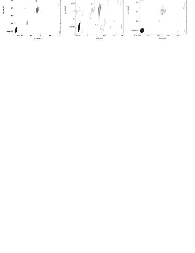
Figure 2: Left panel: VLA radio continuum image of HD 154090 at 8.46 GHz. Contour levels: –0.08, 0.08 ($2\sigma$), 0.12, 0.15, 0.18. and 0.21 mJy beam^-1. Central panel: VLA radio continuum image of HD 76341 at 8.46 GHz. Contour levels: –0.15, 0.15 ($3\sigma$), 0.2, 0.25, 0.3 and 0.35 mJy beam^-1. Right panel: ATCA radio continuum image of HD 148379 at 17.8 GHz. Contour levels: –0.1, 0.15 ($3\sigma$), 0.2, 0.25, and 0.3 mJy beam^-1. The optical position of the star is marked with a cross, and the synthesized beam is displayed in the bottom left corner of each image.

Table 1: Observations details

Star	Phase	Tel.	Int.	Synth.
	Cal.		time	beam
			(h)	(arcsec)
HD 42087	0559+238	VLA	0.81	$2.2\times 1.8$
HD 43384	0559+238	VLA	0.83	$2.2\times 1.8$
HD 47432	0641-033	VLA	0.75	$2.5\times 2.3$
HD 76341	0828-375	VLA	0.50	$11.3\times 2.3$
HD 112244	j1326-5256	ATCA	3.18	$0.8\times 0.4$
HD 148379	1600-44	ATCA	3.58	$1.0\times 0.8$
HD 154090	1626-298	VLA	0.75	$7.3\times 2.6$
HD 156154	1744-312	VLA	0.5	$7.8\times 2.6$
HD 157246	1657-56	ATCA	6.9	$0.6\times 0.5$
HD 165024	1740-517	ATCA	6.36	$0.7\times 0.5$
HD 204172	2052+365	VLA	1.25	$3.0\times 2.7$
BD-11 4586	1832-105	VLA	0.5	$3.8\times 2.7$

3.2 VLA data

The VLA targets were observed on September 9 and 17, 2005, at C array, during a total observing time of 8 h. The flux density calibrator was 1331+305 ($S_{\rm 3.5cm}=$ 5.23 Jy). The integration time on source, synthesized beam, and phase calibrator corresponding to each source are given in Table 1. The observations were carried out at 3.5 cm with two IF pairs of 50 MHz bandwidth, to obtain a reasonable angular resolution with a moderate amount of calibration time, and lower noise receivers.

The data was reduced and analyzed with the aips and miriad routines. Two stars were detected above the noise: HD 76341, and HD 154090, with signal-to-noise ratio $\geq$ 6 (see Figure 2). The stellar field of HD 156154 showed weak emission at a 3-$\sigma$ level, and a 2-$\sigma$ (probable) noise source coincident with the stellar position. Diffuse emission over the field of HD 42087 precluded the detection of the stellar wind, also superposed to a 2MASS source, and the infrared source IRAS 06066+2307.

An extended source was discovered in the stellar field of BD-11 4586, centered at $(RA,Dec)_{\rm J2000}=(18^{\rm h}18^{\rm m}6.744^{\rm s},-11^{\circ}18^{\prime}16.83^{\prime\prime})$, with a total flux density of 2.8 mJy. No correlation at any wavelength was found for this source in the literature.

3.3 Previous radio observations

We searched the literature for continuum radio observations of late OB supergiants with spectral types between O8 to B3. Among the contributions considered, the comprehensive study by Bieging et al. (1989) on OB stars listed high-resolution radio observations of 16 such supergiants, six of which were detected. Lamers & Leitherer (1993) presented seven radio detections. Scuderi et al. (1998) obtained radio flux densities -or upper limits- for ten candidates. We have also included isolated results from Stevens (2006) (private communication), Benaglia et al. (2001), and the latest radio flux densities detected by Puls et al. (2006) on two O9.5 targets. From the older studies (Bieging et al. 1989, Lamers & Leitherer 1993), only detections were included, as the observations were carried out using the former VLA less sensitive receivers. The star HD 193237 (observations by Scuderi et al. 1998) is to be discussed elsewhere amongst LBVs. The star HD 152408 is not included within the present sample due to its ambiguous classification as either “O8 Iafpe” or “WN9 ha” (Bohannan & Crowther 1999).

The star HD 149404 is listed by Lamers & Leitherer (1993). It has been studied by Rauw et al. (2001), and Thaller et al. (2001), through optical spectroscopy. They found evidences of a binary system, formed by an O7.5 I(f) and an ON9.7 I, with a period of $\sim$ 9 d. Most of the radio emission would be produced in a colliding wind region; the results are consistent with a picture where the secondary star is undergoing Roche lobe overflow. Within this scenario, the radio flux density measured should come from the region of colliding winds, as well as the winds of both components. The mass-loss rate derived from the radio flux density is thus only an upper limit and we disregard from our upcoming analysis this object as well.

Table 2: Supergiants with radio observations: measurements

Star	Sp. Class.	Observ.	$V$, $B$	$v_{\rm w}$	$M_{\rm V}$	$d$	$e_{d}$	$\nu$	$S_{\nu}$	$e_{S}$
				(km s-1)		(kpc)	(kpc)	(GHz)	(mJy)	(mJy)
HD 42087	B2.5 Iba	this work	5.76, 5.96b	735c	-6.4d	1.4e	0.3	8.640	$<$ 0.14
HD 43384	B3 Iabf	this work	6.26, 6.71g	760c	-7.2d	1.4e	0.3	8.640	$<$ 0.24
HD 47432	O9.7 Ibh	this work	6.22, 6.36i	1590c	-6.28j	1.7e	0.4	8.640	$<$ 0.15
HD 76341	O9 Ibk	this work	7.16, 7.46i	1520c	-6.29j	1.9e	0.4	8.640	0.38	0.05
HD 112244	O8.5 Iab(f)l	this work	5.38, 5.40i	1575c	-6.29j	1.5e	0.3	17.79	$<$ 0.3
HD 148379	B1.5 Iapem	this work	5.34, 5.80n	510c	-7.5d	1.3e	0.3	17.79	0.28	0.05
HD 154090	B0.7 Iad	this work	4.87, 5.13d	915d	-6.8d	1.1d	0.3	8.640	0.23	0.04
HD 156154	O8 Iab(f)l	this work	8.05, 8.65i	1530o	-6.3j	2.2e	0.5	8.640	$<$ 0.15
HD 157246	B1 Ibm	this work	3.34, 3.21b	735c	-6.8d	1.1e	0.2	17.79	$<$ 0.18
HD 165024	B2 Ibm	this work	3.66, 3.58b	1185c	-7.2d	0.8e	0.2	17.79	$<$ 0.18
HD 204172	B0 Ibh	this work	5.94, 5.84p	1685c	-6.4d	3.0e	0.7	8.640	$<$ 0.08
BD-11 4586	O8 Ib(f)q	this work	9.4, 10.4i	1530o	-6.3j	1.8e	0.4	8.640	$<$ 0.3
HD 2905	BC 0.7 Iad	SPS98	4.16, 4.30d	1105d	-7.1d	1.1d	0.3	8.450	0.4	0.03
HD 30614	O9.5 Iad	SPS98	4.29, 4.33i	1560d	-6.6d	1.0d	0.2	14.95	0.65	0.13
HD 37128	B0 Iad	SPS98	1.70, 1.51d	1910d	-6.3d	0.4d	0.1	14.95	1.4	0.1
HD 37742	O9.7 Ibr	LL93	1.76, 1.55i	1860c	-6.3j	0.4e	0.1	8.000	0.89	0.04
HD 41117	B2 Iad	SPS98	4.63, 4.91d	510c	-7.6d	1.5d	0.4	14.95	0.63	0.13
HD 80077	B2 Ia+s	LCK95	7.56, 8.90t	140t	-7.2t	3.0p	1.2	8.640	0.5	0.11
HD 151804	O8 Iafl	LL93	5.22, 5.26u	1445c	-6.3j	1.9v	0.3	4.800	0.4	0.1
HD 152236	B1.5 Ia+d	Ste06	4.73, 5.21d	390d	-8.8d	2.0d	0.3	8.640	2.4	0.1
HD 152424	OC9.7 Iar	LL93	6.31, 6.71i	1760c	-6.3j	1.7e	0.4	8.000	0.21	0.04
HD 163181	BN0.5 Iapw	BCK01	6.60, 7.15x	520c	-6.1d	1.6e	0.4	8.640	0.44	0.05
HD 169454	B1 Iay	BAC89	6.65, 7.39x	850z	-6.8d	0.9e	0.2	15.00	1.9	0.1
HD 190603	B1.5 Ia+d	SPS98	5.65, 6.19d	485d	-7.5d	1.5e	0.4	14.95	$<$ 0.7
HD 194279	B2 Iad	SPS98	7.05, 8.07d	550d	-7.0d	1.2d	0.3	8.450	0.44	0.1
HD 195592	O9.5 Il	SPS98	7.08, 7.95i	1765o	-6.3j	1.0e	0.2	14.95	0.9	0.13
HD 198478	B2.5 Iad	SPS98	4.86, 5.28d	470d	-6.4d	0.8d	0.2	8.450	$<$ 0.27
HD 209975	O9.5 Ibz	PMS06	5.10, 5.18i	2050z	-5.45z	0.8z	0.2	14.94	0.422	0.12
CygOB2-10	O9.5 Iz	PMS06	9.88 11.47α	1650z	-6.95z	1.7z	0.2	14.94	0.3	0.1
BD-14 5037	B1.5 Iaβ	SPS98	8.22, 9.58x	750o	-7.4o	1.0e	0.2	14.95	1.1	0.2

^aPerryman et al. 1997, ^bJohnson et al. 1966, ^cHowarth et al. 1997, ^dCrowther et al. 2006, ^ederived with chorizos: see text, ^fLesh et al. 1968, ^gMoffett & Barnes 1979, ^hWalborn 1976, ⁱGOS Catalogue (Maíz Apellániz et al. 2004), ^jMartins et al. 2005, ^kGarrison et al. 1977, ^lWalborn 1973, ^mHiltner et al. 1969, ⁿFeinstein & Marraco 1979, ^oPrinja et al. 1990, ^pCrawford et al. 1971, ^qWalborn 1982, ^rWalborn 1972a, ^sLeitherer et al. 1995 (LCK95), ^tSchild et al. 1983, ^uBohannan & Crowther 1999, ^vHumphreys 1978, ^wWalborn 1972b, ^xKozok et al. 1985, ^yBieging et al. 1989 (BAC89), ^zPuls et al. 2006 (PMS06), ^αMassey & Johnson 1991, ^βMorgan et al. 1955. SPS98: Scuderi et al. 1998. LL93: Lamers & Leitherer 1993. Ste06: I.R. Stevens (private communication). BCK01: Benaglia et al. 2001.

3.4 Considerations on radio-detectability

The O8 to B3 supergiant sample comprises 19 detections (up to 3 mJy) plus upper limits to 11 sources (typically below 0.3 mJy). With the aim of comparing the different radio flux densities measured towards the sample stars, we have extrapolated the values of $S_{\nu}$ to a unique frequency of 14.95 GHz, assuming that the thermal flux behaves as $S_{\nu}\propto\nu^{0.7}$ (Setia Gunawan et al. 2000, Williams 1996). In Figure 3 we have plotted the quantity $S_{\nu}*(d/{\rm 1kpc})^{2}\propto L$ as a function of the stellar effective temperature. We found no correlation of the corrected flux with stellar effective temperature, although the errors in stellar distances are strongly affecting the result.

No correlations between radio flux density and terminal velocity, distance or visual magnitude were found, as expected.

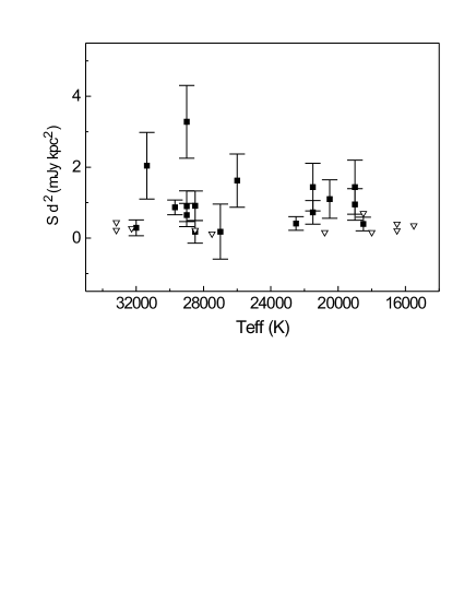
Figure 3: Radio flux density corrected for the stellar distance, as a function of effective temperature. The squares represent detected stars, whilst the triangles represent radio flux density upper limits. The star HD 80077 was excluded due to its large error in distance ($\sim$40%).

4 Stellar parameters and mass-loss rates

Table 2 lists the 30 selected stars in two groups (observed by us, and compiled from the literature), ordered by HD number, together with other observational stellar parameters.

The spectral types for O stars were taken from the GOS catalogue (Maíz Apellániz et al. 2004), Crowther et al. (2006), and Puls et al. (2006). The various references on spectral types of B stars can be seen in Table 2. The $V,B$ and absolute adopted magnitudes are also given.

Most of the stellar wind terminal velocities quoted were published by Howarth et al. (1997). For four objects, the values were taken from the interpolations by Prinja et al. (1990), their Table 3, and involved relatively large errors. For the rest, we have adopted errors of 10%.

Figure 4: The adopted stellar effective temperatures as a function of spectral type, for OB supergiants. The straight line represents the fit $y=37327(\pm 387)-1583(\pm 44)x$, where $x$ is an index running on the different spectral types (from 2 to 14), and $y=T_{\rm eff}$.

To achieve the goal of a uniform database, we have established a common temperature scale for O8-B3 supergiants, re-derived the stellar distances, and calculated the mass-loss rates for all stars in the sample using those consistent parameters.

The effective temperature scale was established taking into account the latest work by Crowther et al. (2006) for individual cases whenever possible, and also from interpolation using their Table 4. For some O supergiants the values were taken from the models by Martins et al. (2005). Isolated values are from Lamers & Leitherer (1993) and Puls et al. (2006). The resulting scale is shown in Figure 4. We have assigned to the thirteen different spectral types and subtypes covered, from O8 to B3, a correlated number (from 2 to 14). Figure 4 plots the stellar effective temperature as a function of this integer number. Spectral types were used to derive temperatures for the stars in the sample. The uncertainties introduced by the discrete nature of the spectral classification scheme, the current state of the art of hot-star atmosphere modeling, and the possible slight mis-classifications are expected to be of the order of 2000 K for late-O stars and 1500 K for early-B stars. The effective temperature adopted for each star is listed in Table 3.

References for the adopted stellar luminosities are quoted in Table 3. The effective temperature and luminosity of HD 42987, HD 148379, and HD 151804 have been derived specifically for this work by means of H$\alpha$ profile fitting (see Section 7).

In order to derive the stellar masses, needed in turn to obtain predicted mass-loss rates (see Section 6), we used the calibration of surface gravity ($g$) with effective temperature published by Crowther et al. (2006) (see their Figure 1, which was built using SMC data presented by Trundle & Lennon 2004). The likely range in the stellar mass for each star can be derived allowing a deviation by up to 0.2 dex in $\log(g)$.

Table 3: Adopted stellar parameters and results

Star	Sp. type	$T_{\rm eff}$	$\log(L_{*}/{\rm L}_{\odot})$	$log(g)$	$M_{*}$	$\eta$	$\dot{M}$	$e_{\dot{M}}$	$\dot{M}_{\rm pred}$	$\dot{M}_{\rm H\alpha}$
		(K)			(M⊙)		(   $10^{-6}\,\,\,\,\,\,$M${}_{\odot}\,\,\,\,\,\,$ yr${}^{-1}\,\,\,$)
HD 156154	O8 Iab(f)	33179a	5.68a	3.10	19.2		$<$ 4.4		3.2
HD 151804	O8 Iaf	29000b	5.88b	3.00	41.4	$1.0\pm 0.12$	10.4	3.70	3.2	16.0b
BD-11 4586	O8 Ib(f)	33179a	5.68a	3.10	19.2		$<$ 5.6		3.2	(2.6)c
HD 112244	O8.5 Iab(f)	32274a	5.65a	3.10	20.0		$<$ 3.0		2.6
HD 76341	O9 Ib	31368a	5.61a	3.05	18.2	$1.3\pm 0.17$	7.2	2.51	2.1
CygOB2-10	O9.5 I	29700d	5.82d	3.00	32.8	$0.5\pm 0.07$	4.4	1.77	2.7	2.7d,e
HD 195592	O9.5 I	29000f	5.60f	3.00	21.7	$1.0\pm 0.14$	4.8	1.69	1.2	3.8d
HD 30614	O9.5 Ia	29000f	5.63f	3.00	23.3	$0.6\pm 0.08$	3.3	1.22	1.5	5.0f
HD 209975	O9.5 Ib	32000d	5.31d	3.10	9.5	$1.2\pm 0.15$	2.4	0.94	0.7	1.1d
HD 37742	O9.7 Ib	28500f	5.57a	2.95	19.4	$0.4\pm 0.05$	1.5	0.49	0.9	(1.8)g
HD 47432	O9.7 Ib	28500f	5.57a	2.96	19.8		$<$ 3.1		1.1	(1.9)h
HD 152424	OC9.7 Ia	28500f	5.57a	2.96	19.8	$1.0\pm 0.14$	4.5	1.65	1.0
HD 37128	B0 Ia	27000f	5.44f	2.90	15.9	$0.5\pm 0.07$	1.6	0.54	0.5	2.3f
HD 204172	B0 Ib	27500f	5.50f	2.93	18.2		$<$ 5.0		0.7
HD 163181	BN0.5 Iap	26000f	5.57a	2.85	22.4	$0.1\pm 0.02$	2.1	0.73	2.5
HD 154090	B0.7 Ia	22500f	5.48f	2.60	18.1	$0.2\pm 0.03$	1.3	0.48	3.2	1.0f
HD 2905	BC0.7 Ia	21500f	5.52f	2.53	20.3	$0.4\pm 0.05$	2.5	0.84	2.3	2.0f
HD 169454	B1 Ia	21500f	5.45f	2.53	17.3	$0.5\pm 0.06$	3.4	1.14	2.9
HD 157246	B1 Ib	20800i	5.45f	2.45	16.4		$<$ 0.6		3.4
BD-14 5037	B1.5 Ia	20500f	5.60f	2.45	24.5	$0.2\pm 0.04$	2.5	1.18	4.9	(3.4)j
HD 152236	B1.5 Ia+	18000f	6.10f	2.20	73.4	$0.1\pm 0.02$	8.3	2.70	41.7	6f
HD 190603	B1.5 Ia+	18500f	5.57f	2.25	21.8		$<$ 2.1		6.8	2.5f
HD 148379	B1.5 Iape	18500b	5.56b	2.25	21.3	$0.1\pm 0.01$	0.8	0.29	5.8	1.5b
HD 194279	B2 Ia	19000f	5.37f	2.30	13.9	$0.2\pm 0.02$	1.5	0.58	3.3	1.1f
HD 41117	B2 Ia	19000f	5.65f	2.30	26.4	$0.1\pm 0.02$	2.1	0.76	8.5	1.0f
HD 80077	B2 Ia+	18500f	5.40f	2.25	14.7	$0.1\pm 0.01$	1.7	0.69	30.2
HD 165024	B2 Ib	18000f	5.40f	2.20	14.7		$<$ 0.6		0.9
HD 198478	B2.5 Ia	16500f	5.03f	2.05	6.3		$<$ 0.5		1.1	0.2f
HD 42087	B2.5 Ib	19000b	5.08b	2.30	7.1		$<$ 1.1		0.9	0.2b
HD 43384	B3 Iab	15500f	4.88h	1.95	4.4		$<$ 1.7		0.3	(0.3)h

^aMartins et al. 2005, ^bthis work, ^cScuderi et al. 1992, ^dPuls et al. 2006, ^eHerrero et al. 2002, ^fCrowther et al. 2006, ^gLamers & Leitherer 1993, ^hMorel et al. 2004, ⁱLamers et al. 1995, ^jScuderi et al. 1998.

Distances were derived using chorizos (Maíz Apellániz 2004) by comparing the observed with $BVJHK_{s}$ photometry with low-gravity Kurucz atmospheres. The temperature for each star was taken from Table 3 and both $E_{4405-5495}$ and $R_{5495}$ (the monochromatic equivalents to $E_{B-V}$ and $R_{V}$, respectively, were left as free parameters. chorizos is a Bayesian code that finds all the solutions for the general inverse photometric problem in which $N$ parameters (two in this case) are fitted to $M$ independent colors (three in this case). After applying chorizos to obtain the unextinguished photometry, the spectroscopic distance was calculated using the values of $M_{V}$ in Table 2, assuming uncertainties between 0.5 and 1.0 magnitudes depending on the spectral type. In all cases we found that the largest contribution to the final uncertainty in the distance, $e_{d}$, is that of the uncertainty in $M_{V}$ and not that of the photometry itself.

We investigated the membership of the sample stars to stellar clusters or OB associations. For those stars belonging to stellar groups, we found that in most cases, our obtained individual distances agree well between errors, with those of the clusters/associations. For the star HD 151804, catalogued as a member of Sco OB1 (Humphreys 1978, $d=1.91$ kpc), the association distance was adopted. Very recently, the distance to HD 169454 was established as 1.36 kpc (Hunter et al. 2006). For the sake of consistency, we have adopted the distance derived here.

In order to derive the radio mass-loss rate values for previously observed stars, we have taken into account the radio flux density at the highest frequency whenever possible (see Table 2).

All mass-loss rates values were derived using Eq. (1), and assuming the measured flux density is thermal. This looks like a reasonable hypothesis, as all but one star (HD 151804) were observed at $\nu\geq 8$ GHz. Besides, the sample stars that have been observed by Bieging et al. (1989) and Scuderi et al. (1998) at more than one frequency, have shown thermal emission. For all but one star we have adopted abundances of $Y_{\rm H}=0.85$, $Y_{\rm He}=0.15$, and assumed that at the temperatures considered, all H is ionized, while He is singly ionized. Consequently $\mu=1.45$, $Z=\gamma=1$. The differences in the mass-loss rate results in considering $\mu=1.3$ – 1.6 were lower than 12%. If the He is doubly ionized in O stars, the mass-loss rates derived here are underestimated by about 30%, although we find this unlikely given the stellar effective temperatures involved. For HD 151804, we adopted $Y_{\rm He}=0.25$. Errors in $\mu$, $Z$, and $\gamma$ were taken as 10%; $\sigma_{L}=0.5L_{*}$. Mass-loss rate values and the corresponding errors derived from error propagation in Eq. (1) are listed in Table 3, and plotted in Fig. 5. In the case of the non-detections, a 3-$\sigma$ flux density upper limit was used, and the corresponding mass-loss rates are upper limits.

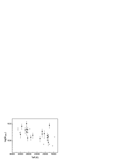
Figure 5: Mass loss rates derived from radio continuum observations, as a function of effective temperature (squares), and upper limits (open triangles).

5 Wind efficiencies

In order to better compare radio results with results from other wavelengths or models, we proceeded to compute the wind efficiencies corresponding to the radio mass-loss rates. The values are shown in Table 3, and in Figure 6 with filled squares. At $T_{\rm eff}\approx 21.5$ kK there are two (squares) stars with wind efficiencies well above those of their neighbours: HD 169454 and HD 2905. The star HD 169454 has been represented twice, for wind efficiencies derived according to two possible distances (see Sect. 4): with a square when the distance adopted here is used, and with a triangle when the Hunter et al. (2006) value is used.

Figure 6: Observed wind efficiency versus effective temperature (squares). Crosses represent ‘corrected’ values (see text). The triangle corresponds to the star HD 169454 if the Hunter et al. (2006) distance is considered. Note the possible presence of a local maximum at the predicted position of the BSJ.

We wish to check if the empirical shapes of the wind efficiency could be an artifact of the fact that we observe objects with different masses and luminosities. This necessarily introduces a scatter in $\eta$, but we may be able to correct for this. The correction was derived in the following manner. From models for different parameter sets of ($M_{*}$, $L_{*}$), we obtain the corresponding wind efficiencies. We choose a parameter set for which $\eta=1$ for the maximum effective temperature and $v_{\infty}/v_{\rm esc}$ ratio (see Fig. 6 from Vink et al. 2000a). The $\eta$ values were plotted as a function of their Eddington factor ($\propto M_{*}/L_{*}$), resulting in Eddington-corrected $\eta$ values (Fig. 7). For each target star we can compute the $\eta$ correction value according to its Eddington factor, and divide the uncorrected $\eta$ by the correction value. The results are also shown in Figure 6. Though an additional source of scatter is being introduced as a result of this via the errors in stellar masses (not shown in the Figure), the ‘corrected’ wind efficiencies are similar to the original values. Consequently, hereafter we will use non-corrected values.

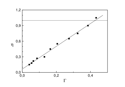
Figure 7: Wind efficiencies taken for the twelve models from Fig. 5 from Vink et al. (2000a), as a function of the Eddington factor $\Gamma$. The straight line represents unity.

5.1 The empirical wind-momentum relation

The radio observations allowed us to estimate the mass-loss rates for the 19 detected stars in a uniform way. We have utilised this database to provide a radio derived calibration for the coefficients $D_{0},x$ of the wind momenta-luminosity relation (WLR; see Kudritzki & Puls 2000) for late O (O8-O9) and B0 supergiants. Our WLR is shown in Figure 8. If the wind momenta equal $D=\dot{M}_{*}\,v_{\infty}\,(R/{\rm R}_{\odot})^{1/2}$, and $\log(D)=D_{0}+x\log(L/{\rm L}_{\odot})$, a linear fit yields the values $D_{0}=26.6\pm 2.1$; $x=1.0\pm 0.4$ when only the O stars (O8-O9) are included, and $D_{0}=25.0\pm 2.7$; $x=1.3\pm 0.5$ when the B0 stars are also included in the fit. For obvious reasons B1 stars are excluded as they are located at the BSJ, whilst for spectral types later than B1, we have too few datapoints to derive a reliable WLR.

We note the shallow slope of our derived WLR. For early-type O stars the slope, $x$, is significantly larger. In standard radiation-driven wind theory, the slope, $x$, is the reciprocal value of the “effective” CAK force multiplier $\alpha_{\rm eff}$ (see Kudritzki & Puls for definitions). For early O-stars, this value is approximately 2/3, the reason for which the stellar mass cancels and the WLR can be used in the first place.

Here, we find an empirical $\alpha_{\rm eff}$ in the range 0.78-1 for O8-B0 stars, which may be consistent with the high $\alpha$ value of $\alpha^{\rm MC}=0.85$ predicted through Monte Carlo simulations by Vink et al. (1999) for models at $T_{\rm eff}=30\leavevmode\nobreak\ 000$K. A high value of $\alpha_{\rm eff}$ may suggest a relatively large value for the ratio of ($v_{\infty}/v_{\rm esc}$). Interestingly objects in this temperature range indeed show the largest ($v_{\infty}/v_{\rm esc}$) ratio according to Fig. 6 of Kudritzki & Puls (2000). We note however that for these large values of $\alpha_{\rm eff}$ (when $\alpha_{\rm eff}$ no longer equals 2/3), the concept of the WLR may lose its meaning. Investigations of the wind efficiency $\eta$ versus temperature may therefore be a more valuable tool to understand wind driving for different effective temperature regimes.

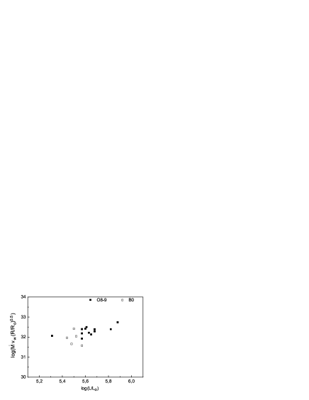
Figure 8: Wind momenta $D$ of galactic late O-, and early B supergiants as a function of luminosity, derived using radio continuum observations.

6 Mass-loss rates: expected versus predicted

Once we have estimated the wind efficiencies from mass-loss rates derived using radio flux densities, we proceeded to compare the results with model predictions. Vink (2000), and Vink et al. (2000a) developed mass-loss rate models and presented them for a $(L_{*},M_{*})$ grid. Based on the models, they produced a recipe to derive a stellar mass-loss rate if the stellar mass, luminosity, effective temperature and terminal velocity are known. We have made use of the routine to derive the expected mass-loss rates for the radio observed stars. The program also provides information on the position of the star with respect to the BSJ, according to the specific stellar parameters. The predicted mass-loss rates $\dot{M}_{\rm pred}$ are given in Table 3.

The recipe to derive the predicted mass-loss rates has helped to discriminate which stars are above and below the BSJ temperature, and we divided them into two groups. Both groups consist of 15 stars. The first group contains: HD 30614, HD 37128, HD 37742, HD 47432, HD 76341, HD 112244, HD 152424, HD 156154, HD 151804, HD 163181, HD 195592, HD 209975, HD 204172, BD-11 4586, and Cyg OB2 No. 10. The second group contains the remaining 15 objects.

The errors involved in the derivation of the predicted mass-loss rates are $\sigma_{L_{*}}=0.5\,L_{*}$, 0.2 dex in $\log(g)$, and $\sigma_{T{\rm eff}}=2000-1500$ K. A direct comparison between expected and measured values is presented in Figure 9. We show the wind efficiencies derived using radio observations towards Galactic stars, and, superposed, the predicted wind efficiency number constructed for $\log(L_{*}/{\rm L_{\odot}})=6.0$, $M_{*}=60$ M_⊙, $v_{\infty}/v_{\rm esc}=2.6$, as in Fig. 1.

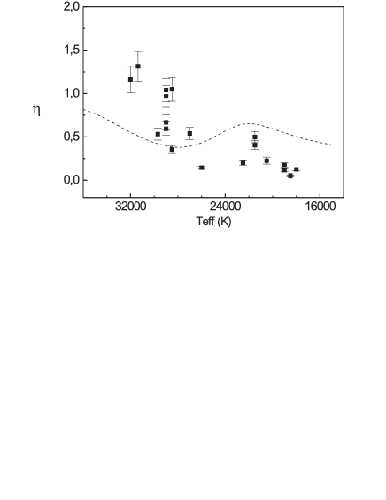
Figure 9: Modelled wind efficiency for $\log(L/{\rm L_{\odot}})=6.0$, $M_{*}=60$ M_⊙, $v_{\infty}/v_{\rm esc}=2.6$ (dashed line, same as in Fig. 1) superposed to the wind efficiencies derived by means of radio observations, for Galactic stars (squares).

Our results show that the stars above the BSJ temperature have predicted mass-loss rates lower than the empirical radio mass-loss rates. The reverse holds true for the stars below the BSJ temperature. If the radio mass-loss rates are affected by significant wind clumping, these empirical rates may need to be reduced by a certain amount, and possibly be brought into agreement with the predictions of radiation-driven wind models. If for stars above the BSJ temperature, the discrepancy between the empirical rates and the theoretical rates is attributable to wind clumping overestimating empirical rates – whilst the theoretical rates are not affected – then, adopting a similar clumping correction for stars below the BSJ temperature, would worsen the discrepancy between the empirical and theoretical rates for B supergiants.

The reader should be aware that our analysis has been performed using derived mass-loss rates only. “Upper limits” are not taken into account in the comparison between empirical radio rates and mass-loss predictions. Therefore our comparison on the absolute value of the mass-loss rate is necessarily incomplete. Having noted this, there is no a priori reason why incompleteness should be a function of stellar temperature, and although the issue of the absolute mass-loss rates of hot-star winds is still an open one, the qualitative comparison between the empirical radio mass-loss rates and the Monte Carlo predictions of radiation-driven wind models appears to support the predicted mass-loss BSJ. More data around the BSJ will be necessary to confirm this.

7 Comparison of radio and H$\alpha$ results

Many of the stars composing our sample have mass-loss rates in common with measurements from H$\alpha$ profiles. The values of $\dot{M}_{\rm H\alpha}$ are listed in Table 3, with their references (Lamers & Leitherer 1993; Scuderi et al. 1992, 1998; Puls et al. 2006; Crowther et al. 2006; Morel et al. 2004; Herrero et al. 2002).

Additionally, three new H$\alpha$ mass-loss rates have been derived specifically for this work. The stars HD 42087, HD 148379, and HD 151804 were analyzed in an identical manner to Crowther et al. (2006). For the first two stars the analysis was based on VLT/UVES data (PoP Survey, Bagnulo et al. 2003). For HD 151804, AAT/UCLES spectroscopy was used, and the data was re-analyzed using current version of code plus TLUSTY velocity structure at depth. Figure 10 displays the H$\alpha$ profile of HD 148379 with errors, showing the reliability with which mass-loss rates can be achieved.

Figure 10: H$\alpha$ profile of HD 148379. Source: UVES PoP Survey.

Figure 11 presents the wind efficiencies derived using mass-loss rates from H$\alpha$ profiles for 20 stars out of the present sample (see Table 3). Results from for modern cmfgen and fastwind profile fitting are represented with filled squares. The rest (open squares) are specified in Table 3 with brackets. The results with $T_{\rm eff}$ are more scattered than they were for the radio wind efficiencies, but they do not contradict the predicted behaviour.

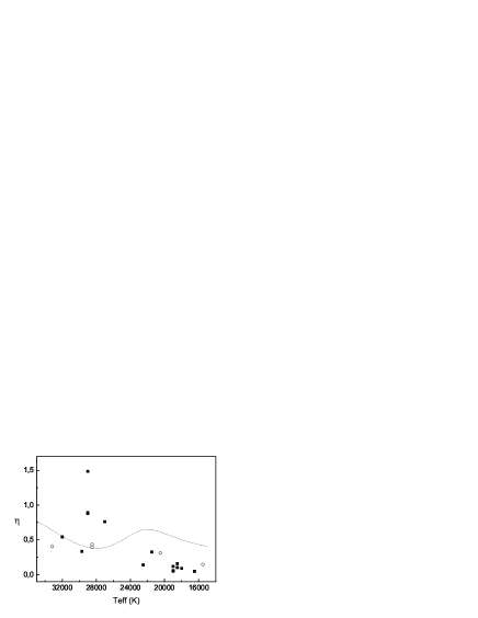
Figure 11: Wind efficiencies from H$\alpha$ measurements for the sample stars. Filled squares: results from cmfgen/fastwind profile fitting. Open squares: results from other methods. Dashed line: same as Figure 1.

An analogous plot to the Galactic H$\alpha$ one can be constructed for extragalactic stars. Trundle et al. (2004), and Trundle & Lennon (2005) have obtained the mass-loss rates of 16 B supergiants earlier than B4 in the Small Magellanic Cloud, by means of H$\alpha$ measurements, all treated in a homogeneous way. These $\dot{M}_{{\rm H}_{\alpha}}$ are shown in Figure 12, as a function of the temperature scale adopted in this work. Possibly, the wind efficiencies for some stars around 22 000 K are above the overall decreasing trend, but larger samples are required to test if the SMC mass-loss rates indeed have a local maximum around the BSJ.

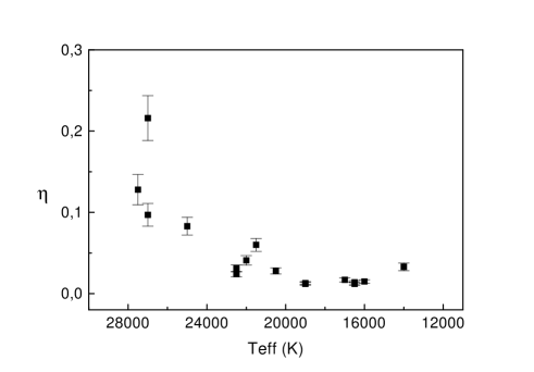
Figure 12: Wind efficiencies from H$\alpha$ measurements for SMC stars (from Trundle et al. 2004, and Trundle & Lennon 2005).

Studies of the comparison between mass-loss rates derived using different methods have been conducted by various groups. Very recently, Fullerton et al. (2006) derived mass-loss rates from UV profiles and investigated whether the UV rates matched those estimated from H$\alpha$ profiles and radio observations. They found that the results follow the relation: $\dot{M}_{\rm UV}<\dot{M}_{\rm H\alpha}<\dot{M}_{\rm radio}$ and attributed this discrepancy to the presence of wind clumping.

In the present study we have assumed that the free-free radio emission is due to smooth winds. If the winds are significantly clumped, the radio-rates derived in our paper are likely overestimates (see e.g. Blomme et al. 2003). We constructed Figure 13 with all radio and H$\alpha$ mass-loss rate results available. From the figure it is clear that there is a good match between both sets of data, although the H$\alpha$ lines are formed in the inner wind, whilst the radio emission arises from the outer wind. This agreement does not necessarily discard clumping, but it may support the hypothesis that the clumping structure is uniformly distributed throughout the whole extension of the wind.

A similar agreement between the inner and the outer wind was found for a large sample of O stars by Lamers & Leitherer (1993). However, these results have been challenged by Fullerton et al. (2006) and Puls et al. (2006).

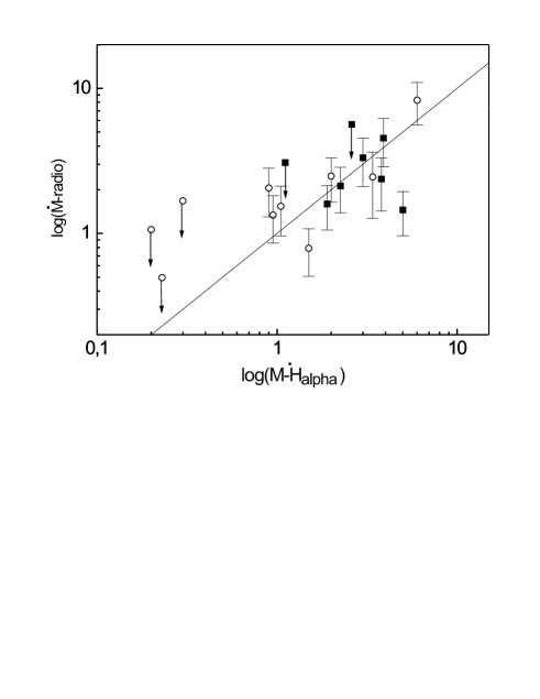
Figure 13: H$\alpha$-derived versus radio-derived mass-loss rates. Units are 10^-6 M$\odot$ yr^-1. Squares: stars above the BSJ temperature; open circles: stars below the jump temperature. Symbols with arrows represent upper limits in $\dot{M}_{\rm radio}$.

8 Summary and conclusions

Throughout the present investigation, a database of radio data of 30 O8-B3 supergiants has been constructed, with observations carried out by different authors. The stellar distances have been reviewed and re-derived, using a subroutine that takes into account the IR and optical indices. We have defined a uniform stellar temperature scale for the spectral range O8-B3.

We have performed high resolution continuum radio observations towards 12 O8-B3 supergiants, detecting three of them: HD 76341, HD 148379 and HD 154090, and derived their mass-loss rates. The rates of another 18 stars were re-determined using results from the literature.

New H$\alpha$ mass-loss rates have been obtained for three objects: HD 42087, HD 148379, and HD 151804. The comparison of mass-loss rates derived from H$\alpha$ and radio observations yielded rather good agreement, contrary to some results from previous investigations. However, we note that there are outliers/significant discrepancies for individual cases.

The renormalization of radio observations allowed us to derive a new calibration for the WLR for supergiants of spectral types in the range O8 to B0.

The comparison between predicted ($p$-values) and radio-derived ($r$-values) mass-loss rates yields different results for stars above and below the BSJ temperature. For the latter group we find $p$-values that are larger than the $r$-values, whilst we find the contrary for the first group. The discrepancy in the first group may be attributed to wind clumping, but this would not explain the discrepancy for the objects below the BSJ temperature. An investigation into the effect of wind clumping on the predictions, for objects both above and below the BSJ temperature, would shed light on this issue.

Our radio study of 30 supergiants of spectral types O8-B3 has revealed that for stars around the BSJ, the wind efficiency appear to be above the predicted general declining function towards later spectral types. The temperature of the potential local maximum also agrees with the predicted temperature of the BSJ. Possibly, a similar behaviour is present for the H$\alpha$ results from SMC stars by Trundle & Lennon (2005).

From the analysis of the WLR obtained here, we found the corresponding empirical CAK force multiplier to lie in the range $\alpha_{\rm eff}=0.78-1$. For these large values of $\alpha_{\rm eff}$, the concept of the WLR may loose its meaning. Studies of the wind efficiency as a function of effective temperature should be considered a powerful alternative to the more often used WLR.

- (1) Abbott, D.C., Bieging, J.H., Churchwell, E., & Cassinelli, J.P. 1980, ApJ, 238, 196
- (2) Bagnulo, S., Jehin, E., Ledoux, C., et al. 2003, Messenger, 114, 10
- (3) Benaglia, P., Cappa, C.E., & Koribalski, B. 2001, A&A, 200, 58
- (4) Bieging, J.H., Abbott, D.C., & Churchwell, E.B. 1989, ApJ, 340, 518
- (5) Blomme, R., van de Steene, G.C., Prinja, R.K., et al. 2003, A&A, 408, 715
- (6) Bohannan, B., & Crowther, P.A. 1999, ApJ, 511, 374
- (7) Bouret, J.,-C., Lanz, T., & Hillier, D.J. 2003, ApJ, 595, 1182
- (8) Castor, J.I., Abbott, D.C., & Klein, R.I. 1975, ApJ, 195, 157
- (9) Chiosi, C., & Maeder, A. 1986, ARA&A, 24, 329
- (10) Crawford, D.L., Barnes J.V., Golson J.C. 1971, AJ, 76, 1058
- (11) Crowther, P.A., & Bohannan, B. 1997, A&A, 317, 532
- (12) Crowther, P.A., Lennon, D.J., & Walborn, N.R. 2006, A&A, 446, 279
- (13) Cure, M., Rial, D.F., & Cidale, L. 2005, A&A, 437, 929
- (14) Davies, B., Vink, J.S., & Oudmaijer, R.D. 2007, A&A, to be submitted
- (15) Eldridge, J.J., & Vink, J.S., 2006, A&A, 452, 295
- (16) Evans, C.J., Lennon, D.J., Walborn, N.R., et al. 2004, PASP, 116, 909
- (17) Eversberg, T., Lépine, S., & Moffat, A.F.J. 1998, ApJ, 494, 799
- (18) Feinstein, A., & Marraco, H.G. 1979, AJ, 84, 1713
- (19) Fullerton, A.W., Massa, D.L., & Prinja, R.K. 2006, ApJ, 637, 1025
- (20) Garrison, R.F., Hiltner, W.A., & Schild, R.E. 1977, ApJS, 35, 111
- (21) Herrero, A., Puls, J., & Najarro, F. 2002, A&A, 396, 949
- (22) Heger, A., Fryer, C.L., Woosley, S.E., et al. 2003, ApJ, 591, 288
- (23) Hillier, D.J., & Miller, D.L. 1998, ApJ, 496, 407
- (24) Hiltner, W.A., Garrison, R.F., & Schild, R.E. 1969, ApJ, 1157, 313
- (25) Howarth, I.D., Siebert, K.W., Hussain, G.A.J., & Prinja, R.K. 1997, MNRAS, 284, 265
- (26) Humpreys, R.M. 1978, ApJS, 38, 309
- (27) Hunter, I., Smoker, J.V., Keenan, F.P., et al. 2006, MNRAS, 367, 1478
- (28) Johnson, H.L., Mitchell R.I., Iriarte B., & Wisniewski W.Z. 1966, Comm. Lunar Plan. Lab. IV, No 63
- (29) Kotak, R., & Vink, J.S. 2006, A&A (Letters), in press
- (30) Kozok, J.R. 1985, AAS, 61, 387
- (31) Kudritzki, R., & Puls, J. 2000, ARAA, 629
- (32) Lamers, H.J.G.L.M., & Pauldrach, A.W.A. 1991, A&A, 244, L5
- (33) Lamers, H.J.G.L.M., & Leitherer, C. 1993, ApJ, 412, 771
- (34) Lamers, H.J.G.L.M., Snow, T.P., & Lindholm, D.M. 1995, ApJ, 455, 269
- (35) Leitherer, C., Chapman, J.M., & Koribalski, B. 1995, ApJ, 450, 289
- (36) Limongi, M., & Chieffi, A. 2006, ApJ, 647, 483
- (37) Lesh, J.R. 1968, ApJ, 517, 371
- (38) Lucy, L.B., & Solomon, P.M. 1970, ApJ, 159, 879
- (39) Maeder, A., & Meynet, G. 2003, A&A, 411, 543
- (40) Maíz-Apellániz, J., Walborn, N.R., Galué, H.A., & Wei, L.H. 2004, ApJS, 151, 103
- (41) Maíz Apellániz, J. 2004, PASP 116, 859
- (42) Markova, N., Puls, J., Repolust, T., & Markov, H. 2004, A&A, 413, 693
- (43) Martins, F., Schaerer D., & Hillier, D.J. 2005, A&A, 436, 1049
- (44) Massey, P., & Thompson, A.B. 1991, AJ, 101, 1408
- (45) Moffett, A.T., & Barnes, T.G. 1979, PASP, 91, 289
- (46) Mokiem, M.R., de Koter, A., Vink, J.S., et al. 2007, A&A, submitted
- (47) Morel, T., Marchenko, S.V., Pati, A.K., et al. 2004, MNRAS, 351, 552
- (48) Morgan, W.W., Code, A.D., & Whitford, A.E. 1955, ApJS, 2, 41
- (49) Panagia, N., & Felli, M. 1975, A&A, 39, 1
- (50) Pauldrach, A.W.A., & Puls, J. 1990, A&A, 237, 409
- (51) Pelupessy, I., Lamers, H.J.G.L.M., & Vink, J.S. 2000, A&A, 359, 695
- (52) Perryman, M.A.C., Lindegren, L., Kovalevsky, J., et al. 1997, A&A, 323, L49
- (53) Prinja, R.K., Barlow, K.J., & Howarth, I.D. 1990, ApJ, 361, 607
- (54) Prinja, R.K., Massa, D., & Searle, S.C. 2005, A&A, 403, L41
- (55) Puls, J., Markova, N., Scuderi, S., et al. 2006, A&A, 454, 652
- (56) Rauw, G., Nazé, Y., Carrier, F., et al. 2001, A&A, 366, 585
- (57) Repolust, T., Puls, J., & Herrero, A. 2004, A&A, 415, 349
- (58) Schild R.E., Garrison R.F., Hiltner W.A. 1983, ApJS, 51, 321
- (59) Scuderi, S., Bonanno, G., di Benedetto, R., et al. 1992, ApJ, 392, 201
- (60) Scuderi, S., Panagia, N., Stanghellini, et al. 1998, A&A, 332, 251
- (61) Setia Gunawan, D.Y.A., de Bruyn, A.G., van der Hucht, K.A., & Williams, P.M. 2000, A&A, 356, 676
- (62) Smith, N., Vink, J.S., de Koter, A. 2004, ApJ, 615, 475
- (63) Thaller, M.L., Gies, D.R., Fullerton, A.W., et al. 2001, ApJ, 554, 1070
- (64) Trundle, C., Lennon, D.J., Puls, J., & Dufton, P.L. 2004, A&A, 417, 217
- (65) Trundle, C., & Lennon, D.J. 2005, A&A, 434, 677
- (66) Vink, J.S. 2000, Ph.D. Thesis, University of Utrecht
- (67) Vink, J.S. 2006, in “Stellar Evolution at Low Metallicity: Mass Loss, Explosions, Cosmology”, Eds. H.J.G.L.M. Lamers, N. Langer, T. Nugis, & K. Annuk, PASP Conf. Ser., 353, 113
- (68) Vink, J.S., & de Koter, A. 2002, A&A, 393, 543
- (69) Vink, J.S., de Koter, A., & Lamers, H.J.G.L.M. 1999, A&A, 350, 181
- (70) Vink, J.S. de Koter, A., & Lamers, H.J.G.L.M., 2000a, A&A 362, 295
- (71) Vink, J.S. de Koter, A., & Lamers, H.J.G.L.M., 2000b, ASPC, 204, 427
- (72) Vink, J.S. de Koter, A., & Lamers, H.J.G.L.M., 2001, A&A 369, 574
- (73) Walborn, N.R. 1972a, AJ, 77, 312
- (74) Walborn, N.R. 1972b, ApJ, 176, 119
- (75) Walborn, N.R. 1973, AJ, 78, 1067
- (76) Walborn, N.R. 1976, ApJ, 205, 419
- (77) Walborn, N.R. 1977, ApJ, 176, 116
- (78) Walborn, N.R. 1982, AJ, 87, 1300
- (79) Williams, P.M. 1996, ASP Conf. Ser. 93, p.15
- (80) Wright, A.E., & Barlow, M.J. 1975, MNRAS, 170, 41