Anisotropy in the Hubble constant as observed in the HST Extragalactic Distance Scale Key Project results

Abstract

Based on general relativity, it can be argued that deviations from a uniform Hubble flow should be thought of as variations in the Universe’s expansion velocity field, rather than being thought of as peculiar velocities with respect to a uniformly expanding space. The aim of this paper is to use the observed motions of galaxies to map out variations in the Universe’s expansion, and more importantly, to investigate whether real variations in the Hubble expansion are detectable given the observational uncertainties. All-sky maps of the observed variation in the expansion are produced using measurements obtained along specific lines-of-sight and smearing them across the sky using a Gaussian profile. A map is produced for the final results of the HST Extragalactic Distance Scale Key Project for the Hubble constant, a comparison map is produced from a set of essentially independent data, and Monte Carlo techniques are used to analyse the statistical significance of the variation in the maps. A statistically significant difference in expansion rate of 9 km s^-1 Mpc^-1 is found to occur across the sky. Comparing maps of the sky at different distances appears to indicate two distinct sets of extrema with even stronger statistically significant variations. Within our supercluster, variations tend to occur near the supergalactic plane, and beyond our supercluster, variations tend to occur away from the supergalactic plane. Comparison with bulk flow studies shows some concordance, yet also suggests the bulk flow studies may suffer confusion, failing to discern the influence of multiple perturbations.

1 Introduction

Conventionally, the Hubble flow is thought of as being completely uniform and isotropic. Deviations from a uniform Hubble flow are eliminated by imparting objects’ observed residual recessional velocities into peculiar velocities, such that objects are thought to move with respect to a uniformly expanding space. However, empirically it is only valid to consider the velocity field of the matter and how everything is moving relative to everything else in the Universe. It is not possible to infer the existence of an absolute space that expands uniformly and that objects have peculiar velocities with respect to. Thus, deviations from a uniform Hubble flow should properly be considered deviations in the Universe’s expansion itself.

Interestingly, RaychaudhuriRay55 (1955) showed that (ignoring vorticity) if a velocity field has locally isotropic expansion, then the space is locally isotropic. Yet we know from examples such as gravitational lensing that inhomogeneities alter the curvature of space such that it is not locally isotropic. Thus, since space is not locally isotropic, then the Universe’s expansion can not be locally isotropic either. Whether to conceive of the Universe expanding non-uniformly or whether to conceive of it expanding uniformly with superimposed peculiar velocities is more than just a conceptual issue, however.

According to Raychaudhuri’s equationRay55 (1955), the existence of shear in a velocity field will lead to a decrease in the volume expansion. Since inhomogeneities should introduce tidal forces and shear the velocity field, then the existence of overdensities and underdensities in the Universe should lead to shear throughout the Universe that decreases the Universe’s volume expansion compared with that of a homogeneous universe. This effect should only be significant when measured locally in the vicinity of an inhomogeneity: the global influence should be quite small. Raychaudhuri’s equation also shows that the existence of vorticity (and also velocity dispersion in the Newtonian version) will lead to an increase in the volume expansion. When structures start to collapse in the Universe and eventually become supported by vorticity or velocity dispersion, those regions of space cease shrinking, which can lead to an increase in the global expansion of the Universe. Thus, it is important to consider the influence inhomogeneities may have on the Universe’s expansion.

The Cosmological Principle—that the Universe is homogeneous and isotropic—is generally assumed to hold, since averaged over large enough scales the Universe will appear homogeneous. However, general relativity is needed to understand not only small dense systems, but large diffuse systems such as the Universe, and according to Einstein’s field equations, the spacetime corresponding to a homogeneous universe can not be used to represent a spatially-averaged inhomogeneous universe. This is because Einstein’s field equations do not equate the spacetime to the mass-energy distribution directly. The energy-momentum tensor $T_{ab}$ depends on the Ricci tensor $R_{ab}$ and scalar $R$, which stem from taking derivatives of the metric tensor $g_{ab}$, with Einstein’s equations equating

$$R_{ab}-\frac{1}{2}Rg_{ab}=\kappa T_{ab}.$$

If the left-hand side of the field equations for a homogeneous universe is equated to the spatially-averaged mass-energy of an inhomogeneous universe, there will generally be a discrepancy between the two sides of the field equations, which will act like a cosmological constant and either accelerate or decelerate the universe’s expansion from that expected for a homogeneous universe. Thus, even if the Universe may look homogeneous on large enough scales, assuming the Universe to expand uniformly is ultimately misleading. Several researchers have suggested this effect may even explain the Universe’s apparent acceleration (reported by Perlmutter et al. Per99, 1999) as being due to structure formation—Bildhauer and FutamaseBil91 (1991), Bene et al.Ben03 (2003), and Kolb et al.Kolb05 (2005)—although Russ et al.Russ97 (1997) argue that the effect of inhomogeneities should be small.

Also, conceiving of the Universe’s expansion as uniform and assigning the galaxies peculiar velocities, bulk flow studies such as that of Hudson et al.Hud04 (2004) have continued to find that the peculiar velocities with respect to the Cosmic Microwave Background (CMB) frame are correlated such that volumes of space of order 100 Mpc in radius are moving with bulk velocities of approximately 300–700 km s^-1. This suggests inhomogeneities significantly perturb the velocity field of the Universe. The existence of the Universe’s large-scale structure of voids and superclusters suggests the voids are underdense regions that have been decelerated less due to gravity so they have ballooned up into roughly spherical regions without undergoing structure formation, while the superclusters are overdense regions where gravity has overcome the Universe’s expansion such that they have reached turnaround and collapsed in their densest regions.

Moffat and TatarskiMof95 (1995) looked at what observational effects we would theoretically observe if we were to inhabit a local void. Via comparison of their theoretical curves with a survey of redshift-distance determinations, they found the data were better fit by a model with a local void than by a homogeneous universe. Zehavi et al.Zeh98 (1998) used 44 type Ia supernova $H_{0}$ values to show that we may just inhabit an underdense region of the Universe (where the expansion in the velocity field has been slowed less due to gravity than in more dense regions of the Universe). Referring to fig. 4 of Freedman et al.Fre01 (2001), it appears that the $H_{0}$ values tend to fall off beyond a distance of 100 Mpc, which suggests the Universe may be expanding faster locally. A here-there difference in the Universe’s expansion could be an alternative to the notion of a now-then difference, which is the assumption the Universe’s supposed acceleration (Perlmutter et al. Per99, 1999) rests on, so it is important to account for the possible influence of inhomogeneities on the Universe’s expansion if the cosmological parameters are to be properly determined.

Thus, in this paper we will not assume the existence of a uniform spatial expansion with peculiar velocities superimposed. We will use $H_{0}$ values measured along different lines-of-sight to see whether local variation in $H_{0}$ exists, and to produce all-sky maps of the observed variation across the sky. If more variation exists in the maps than should be expected due to measurement errors in the data, and if the high and low values of $H_{0}$ are correlated in position on the sky, then this will be taken as evidence that the expansion is indeed locally anisotropic across the sky. Since bulk flow studies find bulk flows of a few hundred km s^-1 on 100 Mpc scales, which is predicted depending on the cosmological model (e.g. see Zaroubi Zar02, 2002), and bulk flows only show the net flow of a sample volume rather than the individual variations in the velocity field, then it would be expected that variations in $H_{0}$ observed on this scale should be at least a few km s^-1 Mpc^-1.

While it is easy enough to measure how fast objects are expanding away from us via redshifts, it is the determination of accurate distances that is problematic in the determination of $H_{0}$. Historically, the errors in $H_{0}$ have been so great that it would be difficult to study real variation in the Universe’s expansion rate. The most accurate work to date to study $H_{0}$ is the HST Extragalactic Distance Scale Key Project (Freedman et al. Fre01, 2001, hereafter the HST Key Project), which yielded distances accurate enough for a meaningful study of real variation in $H_{0}$, especially since most of the errors are systematic and shared by all the $H_{0}$ determinations. Thus, we will map the directional variation in $H_{0}$ using the HST Key Project data, comparing with a second set of data to examine whether the same general trend is observed. The data selection will be discussed in Sect. 2. The technique used to generate all-sky $H_{0}$ maps and study the significance of the variations and the impact of distance will be outlined in Sect. 3. In Sect. 4 the results will be examined from various frames of reference and a comparison with bulk flow studies will be made.

2 Selection of Data

2.1 HST Key Project data

Table 1: HST Key Project $H_{0}$ Data

Object ID	$\alpha$	$\delta$	$H_{0}$
or Cluster	(hours)	(degrees)	(km/s/Mpc)	Reference
SN 1990O	17.15	$+$16.2	67.3 $\pm$ 2.3	Freed. Fre01 (2001)
SN 1990T	19.59	$-$56.2	75.6 $\pm$ 3.1	Freed. Fre01 (2001)
SN 1990af	21.35	$-$62.4	75.8 $\pm$ 2.8	Freed. Fre01 (2001)
SN 1991S	10.29	$+$22.0	69.8 $\pm$ 2.8	Freed. Fre01 (2001)
SN 1991U	13.23	$-$26.1	83.7 $\pm$ 3.4	Freed. Fre01 (2001)
SN 1991ag	20.00	$-$55.2	73.7 $\pm$ 2.9	Freed. Fre01 (2001)
SN 1992J	10.09	$-$26.4	74.5 $\pm$ 3.1	Freed. Fre01 (2001)
SN 1992P	12.42	$+$10.2	64.8 $\pm$ 2.2	Freed. Fre01 (2001)
SN 1992ae	21.28	$-$61.3	81.6 $\pm$ 3.4	Freed. Fre01 (2001)
SN 1992ag	13.24	$-$23.5	76.1 $\pm$ 2.7	Freed. Fre01 (2001)
SN 1992al	20.46	$-$51.2	72.8 $\pm$ 2.4	Freed. Fre01 (2001)
SN 1992aq	23.04	$-$37.2	64.7 $\pm$ 2.4	Freed. Fre01 (2001)
SN 1992au	00.10	$-$49.6	69.4 $\pm$ 2.9	Freed. Fre01 (2001)
SN 1992bc	03.05	$-$39.3	67.0 $\pm$ 2.1	Freed. Fre01 (2001)
SN 1992bg	07.42	$-$62.3	70.6 $\pm$ 2.4	Freed. Fre01 (2001)
SN 1992bh	04.59	$-$58.5	66.7 $\pm$ 2.3	Freed. Fre01 (2001)
SN 1992bk	03.43	$-$53.4	73.6 $\pm$ 2.6	Freed. Fre01 (2001)
SN 1992bl	23.15	$-$44.4	72.7 $\pm$ 2.6	Freed. Fre01 (2001)
SN 1992bo	01.22	$-$34.1	69.7 $\pm$ 2.4	Freed. Fre01 (2001)
SN 1992bp	03.36	$-$18.2	76.3 $\pm$ 2.6	Freed. Fre01 (2001)
SN 1992br	01.45	$-$56.1	67.2 $\pm$ 3.1	Freed. Fre01 (2001)
SN 1992bs	03.29	$-$37.2	67.8 $\pm$ 2.8	Freed. Fre01 (2001)
SN 1993B	10.35	$-$34.3	69.8 $\pm$ 2.4	Freed. Fre01 (2001)
SN 1993O	13.31	$-$33.1	65.9 $\pm$ 2.1	Freed. Fre01 (2001)
SN 1993ag	10.03	$-$35.3	69.6 $\pm$ 2.4	Freed. Fre01 (2001)
SN 1993ah	23.52	$-$27.6	71.9 $\pm$ 2.9	Freed. Fre01 (2001)
SN 1993ac	05.46	$+$63.2	72.9 $\pm$ 2.7	Freed. Fre01 (2001)
SN 1993ae	01.29	$-$01.6	75.6 $\pm$ 3.1	Freed. Fre01 (2001)
SN 1994M	12.31	$+$00.4	74.9 $\pm$ 2.6	Freed. Fre01 (2001)

Table 1: – continued

Object ID	$\alpha$	$\delta$	$H_{0}$
or Cluster	(hours)	(degrees)	(km/s/Mpc)	Reference
SN 1994Q	16.50	$+$40.3	68.0 $\pm$ 2.7	Freed. Fre01 (2001)
SN 1994S	12.31	$+$29.1	72.5 $\pm$ 2.5	Freed. Fre01 (2001)
SN 1994T	13.21	$-$02.1	71.5 $\pm$ 2.6	Freed. Fre01 (2001)
SN 1995ac	22.45	$-$08.5	78.8 $\pm$ 2.7	Freed. Fre01 (2001)
SN 1995ak	02.45	$+$03.1	80.9 $\pm$ 2.8	Freed. Fre01 (2001)
SN 1996C	13.50	$+$49.2	66.3 $\pm$ 2.5	Freed. Fre01 (2001)
SN 1996bl	00.36	$+$11.2	78.7 $\pm$ 2.7	Freed. Fre01 (2001)
Abell 1367	11.74	$+$19.8	75.2 $\pm$ 12.5	Freed. Fre01 (2001)
Abell 2197	16.47	$+$40.9	77.2 $\pm$ 12.5	Sak. Sak01 (2001)
Abell 262	01.88	$+$36.1	70.9 $\pm$ 11.8	Freed. Fre01 (2001)
Abell 2634	23.64	$+$27.0	77.7 $\pm$ 12.4	Freed. Fre01 (2001)
Abell 3574	13.82	$-$30.3	76.2 $\pm$ 12.2	Freed. Fre01 (2001)
Abell 400	02.96	$+$06.6	79.3 $\pm$ 12.6	Freed. Fre01 (2001)
Antlia	10.50	$-$35.3	68.8 $\pm$ 11.3	Freed. Fre01 (2001)
Cancer	08.35	$+$21.0	67.1 $\pm$ 11.0	Freed. Fre01 (2001)
Cen 30	12.77	$-$41.0	75.8 $\pm$ 12.8	Freed. Fre01 (2001)
Cen 45	12.80	$-$40.4	70.7 $\pm$ 11.9	Freed. Fre01 (2001)
Coma	13.00	$+$28.0	83.5 $\pm$ 13.4	Freed. Fre01 (2001)
Eridanus	00.50	$-$21.5	77.6 $\pm$ 12.9	Freed. Fre01 (2001)
ESO 508	13.17	$-$23.1	79.8 $\pm$ 13.0	Freed. Fre01 (2001)
Fornax	03.64	$-$35.5	92.2 $\pm$ 15.3	Freed. Fre01 (2001)
Hydra	10.61	$-$27.5	69.6 $\pm$ 11.1	Freed. Fre01 (2001)
MDL 59	22.01	$-$32.2	73.6 $\pm$ 11.8	Freed. Fre01 (2001)
NGC 3557	11.17	$-$37.5	85.0 $\pm$ 14.4	Freed. Fre01 (2001)
NGC 383	01.12	$+$32.4	73.9 $\pm$ 11.9	Freed. Fre01 (2001)
NGC 507	01.39	$+$33.3	84.9 $\pm$ 13.5	Freed. Fre01 (2001)
Pavo	21.23	$-$57.8	124.4 $\pm$ 19.0	Freed. Fre01 (2001)
Pavo 2	21.23	$-$57.8	86.3 $\pm$ 14.2	Sak. Sak01 (2001)
Pegasus	23.34	$+$08.2	66.4 $\pm$ 10.7	Freed. Fre01 (2001)

Table 1: – continued

Object ID	$\alpha$	$\delta$	$H_{0}$
or Cluster	(hours)	(degrees)	(km/s/Mpc)	Reference
Ursa Major	11.95	$+$49.3	54.8 $\pm$ 8.6	Freed. Fre01 (2001)
Dorado	04.27	$-$55.6	81.9 $\pm$ 8.7	Freed. Fre01 (2001)
Hydra I	10.61	$-$27.5	82.8 $\pm$ 8.4	Freed. Fre01 (2001)
Abell S753	14.06	$-$34.0	87.5 $\pm$ 7.9	Freed. Fre01 (2001)
GRM 15	20.05	$-$55.5	95.6 $\pm$ 10.0	Freed. Fre01 (2001)
Abell 3574	13.82	$-$30.3	92.0 $\pm$ 10.0	Freed. Fre01 (2001)
Abell 194	01.53	$-$01.5	91.3 $\pm$ 7.5	Freed. Fre01 (2001)
Abell S639	10.68	$-$46.2	109.7 $\pm$ 9.9	Freed. Fre01 (2001)
Coma	13.00	$+$28.0	83.2 $\pm$ 6.0	Freed. Fre01 (2001)
DC 2345–28	23.75	$-$28.0	83.2 $\pm$ 6.4	Freed. Fre01 (2001)
Abell 539	05.28	$+$06.5	86.2 $\pm$ 6.5	Freed. Fre01 (2001)
Abell 3381	06.17	$-$33.6	88.9 $\pm$ 8.3	Freed. Fre01 (2001)
NGC 4373	12.42	$-$39.8	99.9 $\pm$ 11.2	Freed. Fre01 (2001)
Abell 262	01.88	$+$36.1	69.0 $\pm$ 7.7	Freed. Fre01 (2001)
Abell 3560	13.53	$-$33.2	78.1 $\pm$ 8.7	Freed. Fre01 (2001)
Abell 3565	13.61	$-$34.0	70.2 $\pm$ 7.8	Freed. Fre01 (2001)
Abell 3742	21.11	$-$47.1	70.0 $\pm$ 7.8	Freed. Fre01 (2001)
Coma	13.00	$+$28.0	70.3 $\pm$ 17.9	Freed. Fre01 (2001)

The HST Key Project data for $H_{0}$ have been selected as the primary data set. This set offers a reasonably large set of values that is distributed nicely for the purpose of making all-sky maps. Also, despite the fact that the $H_{0}$ values depend on the data of other researchers, the values were all analysed by the HST Key Project team to be consistent with each other. Thus, the systematic errors should be similar in most cases to minimize the effect on the study of variations in $H_{0}$ so that most of the uncertainty in the relative values of $H_{0}$ will just be in the random errors.

There are 74 values that were published in the final HST Key Project paper (Freedman et al. Fre01, 2001) as well as 2 values that were obtained from Sakai Sak01 (2001). The data stem from the use of 4 different methods to obtain $H_{0}$: the Tully-Fisher relation, the fundamental plane relation, surface brightness fluctuations, and type Ia supernovae.

In all cases, the $H_{0}$ values used are those for which the recessional velocities have been corrected to the CMB frame. That way the $H_{0}$ values are all in one frame of reference, rather than making corrections for infalls, which would be contrary to our purposes. Thus, the most recent distances from Freedman et al. and Sakai were used, and where $H_{0}$ values corresponding to non-CMB recessional velocities were reported, the CMB-frame recessional velocities from the former papers of Ferrarese et al.Fer00 (2000) and Sakai et al.Sak00 (2000) were used to yield the CMB-frame $H_{0}$ values.

The 2 values obtained from SakaiSak01 (2001) had originally appeared in Sakai et al.Sak00 (2000) but did not appear with modified distances in Freedman et al.Fre01 (2001). One of these values was for Pavo 2, which is a component that was separated from the Pavo Cluster due to some of the galaxies yielding different Tully-Fisher distances, but since the galaxies had similar recessional velocities, they yielded quite different $H_{0}$ values. For our purposes, it only seems fair to include the values for both Pavo components.

Reported in Table 1 are the objects used, their celestial co-ordinates, and their $H_{0}$ values with corresponding 1–$\sigma$ random errors. The celestial co-ordinates for the objects were obtained via SIMBAD.

2.2 Comparison data

Table 2: Comparison $H_{0}$ Data

Object ID	$\alpha$	$\delta$	$H_{0}$
or Cluster	(hours)	(degrees)	(km/s/Mpc)	Reference
Coma	13.00	$+$28.0	71 $\pm$ 30	Her. Her95 (1995)
Coma	13.00	$+$28.0	78 $\pm$ 11	Whit. Whi95 (1995)
Virgo	12.50	$+$13.2	80 $\pm$ 16	Zas. Zas96 (1996)
NGC 7331	22.62	$+$34.4	70 $\pm$ 14	Zas. Zas96 (1996)
Virgo	12.50	$+$13.2	87 $\pm$ 7	Ford Ford96 (1996)
Fornax	03.64	$-$35.5	73 $\pm$ 5	Ford Ford96 (1996)
NGC 5846	15.11	$+$01.6	65 $\pm$ 8	Forb. For96 (1996)
NGC 1365	03.56	$-$36.1	75 $\pm$ 5	Mad. Mad96 (1996)
Coma	13.00	$+$28.0	75 $\pm$ 6	Gregg Gre97 (1997)
IC 4051	13.00	$+$28.0	68 $\pm$ 6	Baum Bau97 (1997)
Coma	13.00	$+$28.0	70 $\pm$ 7	Hjor. Hjo97 (1997)
NGC 4889	13.00	$+$28.0	85 $\pm$ 10	Jen. Jen97 (1997)
NGC 3309	10.61	$-$27.5	46 $\pm$ 5	Jen. Jen97 (1997)
NGC 4881	13.00	$+$28.0	71 $\pm$ 11	Thom. Tho97 (1997)
Abell 2256	17.06	$+$78.7	72 $\pm$ 22	Myers Mye97 (1997)
Coma	13.00	$+$28.0	67 $\pm$ 26	Myers Mye97 (1997)
Abell 262	01.88	$+$36.1	82 $\pm$ 8	Lauer Lau98 (1998)
Abell 3560	13.53	$-$33.2	86 $\pm$ 7	Lauer Lau98 (1998)
Abell 3565	13.61	$-$34.0	83 $\pm$ 6	Lauer Lau98 (1998)
Abell 3742	21.11	$-$47.1	78 $\pm$ 6	Lauer Lau98 (1998)
Coma	13.00	$+$28.0	60 $\pm$ 11	Sal. Sal98 (1998)
PGC 14638	04.20	$-$32.9	60 $\pm$ 15	Pat. Pat98 (1998)
PGC 39724	12.33	$+$29.6	44 $\pm$ 15	Pat. Pat98 (1998)
PGC 51233	14.34	$+$03.9	60 $\pm$ 15	Pat. Pat98 (1998)
PGC 00218	00.05	$+$16.1	58 $\pm$ 15	Pat. Pat98 (1998)
PGC 10208	02.70	$+$00.4	60 $\pm$ 15	Pat. Pat98 (1998)
PGC 35164	11.44	$+$43.6	59 $\pm$ 15	Pat. Pat98 (1998)
PGC 43798	12.89	$+$02.2	39 $\pm$ 15	Pat. Pat98 (1998)
Fornax	03.64	$-$35.5	74 $\pm$ 5	Tul. Tul00 (2000)

Table 2: – continued

Object ID	$\alpha$	$\delta$	$H_{0}$
or Cluster	(hours)	(degrees)	(km/s/Mpc)	Reference
Ursa Major	11.50	$+$55.0	59 $\pm$ 6	Tul. Tul00 (2000)
Pisces Fil.	01.12	$+$32.4	79 $\pm$ 2	Tul. Tul00 (2000)
Coma	13.00	$+$28.0	83 $\pm$ 2	Tul. Tul00 (2000)
Abell 1367	11.74	$+$19.8	77 $\pm$ 2	Tul. Tul00 (2000)
Antlia	10.50	$-$35.3	86 $\pm$ 3	Tul. Tul00 (2000)
Cen 30	12.77	$-$41.0	83 $\pm$ 3	Tul. Tul00 (2000)
Pegasus	23.34	$+$08.2	77 $\pm$ 3	Tul. Tul00 (2000)
Hydra I	10.61	$-$27.5	70 $\pm$ 2	Tul. Tul00 (2000)
Cancer	08.35	$+$21.0	80 $\pm$ 2	Tul. Tul00 (2000)
Abell 400	02.96	$+$06.6	76 $\pm$ 2	Tul. Tul00 (2000)
Abell 2634	23.64	$+$27.0	70 $\pm$ 2	Tul. Tul00 (2000)
Abell 262	01.88	$+$36.1	77 $\pm$ 4	Jen. Jen01 (2001)
Abell 496	04.56	$-$13.2	74 $\pm$ 2	Jen. Jen01 (2001)
Abell 779	09.33	$+$33.8	73 $\pm$ 2	Jen. Jen01 (2001)
Abell 1060	10.61	$-$27.5	74 $\pm$ 4	Jen. Jen01 (2001)
Abell 1656(a)	12.99	$+$28.0	79 $\pm$ 3	Jen. Jen01 (2001)
Abell 1656(b)	12.99	$+$28.0	82 $\pm$ 3	Jen. Jen01 (2001)
Abell 2199	16.48	$+$39.6	71 $\pm$ 2	Jen. Jen01 (2001)
Abell 2666	23.85	$+$27.1	68 $\pm$ 2	Jen. Jen01 (2001)
Abell 3389	06.36	$-$65.0	70 $\pm$ 2	Jen. Jen01 (2001)
Abell 3565	13.61	$-$34.0	78 $\pm$ 4	Jen. Jen01 (2001)
Abell 3581	14.12	$-$27.2	74 $\pm$ 2	Jen. Jen01 (2001)
Abell 3656	19.98	$-$38.3	72 $\pm$ 3	Jen. Jen01 (2001)
Abell 3742	21.11	$-$47.1	81 $\pm$ 4	Jen. Jen01 (2001)
NGC 4073	12.07	$+$01.9	64 $\pm$ 2	Jen. Jen01 (2001)
NGC 4709	12.83	$-$41.4	107 $\pm$ 7	Jen. Jen01 (2001)
NGC 5193	13.53	$-$33.2	85 $\pm$ 6	Jen. Jen01 (2001)
Coma	13.00	$+$28.0	71 $\pm$ 8	Liu Liu01 (2001)

In an effort to test whether variations detected in the HST Key Project data exist independently of this data set, another set of data has been compiled. This data set has been constructed by conducting a literature search for determinations of $H_{0}$ and using papers that report measurements of $H_{0}$ along individual lines-of-sight, include uncertainties, and for which the observed objects are within the distance range of the HST Key Project data. This yields 57 values, which will hereafter be referred to as the comparison values. Reported in Table 2 are the objects used, celestial co-ordinates (obtained via SIMBAD), and $H_{0}$ values with their reported errors.

It should be noted that the comparison values stem from a mixed bag of methods and different researcher analysis; thus, the potential for this set to be corrupted by systematics between values is greater than in the HST Key Project set. Also, various infall corrections have been made, and these are not always clearly stated in the papers, so these values may not consistently be in the CMB frame. One of the comparison values actually stems from a HST Key Project Cepheid distance value, while 4 of the HST Key Project values depend on comparison data surface brightness fluctuation distances, but the data sets are essentially independent.

3 Contour mapping

3.1 Technique

A method is required to generate an all-sky map based on a set of values located at specific positions on the sky. One method would be to fit spherical harmonics; however, this would require more higher order terms than could ever be convenient in order to not force structure into the map from the lower order terms. Our chosen method is to smear the $H_{0}$ values over the sky using a Gaussian profile for each data point.

The Gaussian smearing method involves laying out a grid on the sky and calculating weighted mean values of $H_{0}$ at each grid point, weighting each actual data point in the average according to its angular separation $\theta$ from the grid point such that the weightings fall off as a Gaussian. Thus, the weighting $W$ of each data point is given by

$$W=\frac{1}{\sqrt{2\pi}\sigma}e^{-\theta^{2}/(2\sigma^{2})}$$

with the standard deviation $\sigma$ controlling how broad the smearing is. Contours of constant $H_{0}$ are then interpolated within the grid of averaged $H_{0}$ values to generate contour maps of $H_{0}$. The values are weighted only by their separations, not their uncertainties (the type Ia supernova values are more distant and have smaller uncertainties, but the effect of distance on the map will be specifically explored in Sect. 3.3).

Gaussian smearing succeeds in creating an all-sky map from a sample of data points associated with specific positions on the sky, and it also averages out the impact of errors associated with individual data points so that variations correlated with directions on the sky have the opportunity to manifest themselves. This will be sufficient for studying large-scale variations in $H_{0}$, although there is no hope of studying any variations that do not have a large angular extent, as there is insufficient sky coverage. It should be kept in mind that this method will also smear out the extrema for any actual variation though, so the range of any real variation in the maps will be diminished somewhat.

For the contour maps presented in this paper, while the angular separations are calculated in spherical co-ordinates (using the dot product of unit vectors for the angular positions of the grid points and data points), the grid points are positioned for a cylindrical projection of the sky and are then mapped out in the form of a sinusoidal projection. The sinusoidal projection is a pseudo-cylindrical projection that preserves areas by keeping latitude lines parallel but shortening their length longitudinally according to the sine of the polar angle (or cosine of the declination).

Unless stated otherwise, the grid points are set $1^{\circ}$ apart in right ascension and $1^{\circ}$ apart in declination, as this appears to be a fine enough grid for the purpose of interpolating contours, and the Gaussian weighting profile falls off with a standard deviation of $25^{\circ}$, as this is approximately the typical separation of the real data points and is a sufficiently broad smearing to fill in the holes in the distribution of data on the sky.

Figure 1: Hubble constant contour maps (in Galactic co-ordinates for a sinusoidal projection of the sky) for (a) the 76 HST Key Project $H_{0}$ values and (b) 57 comparison $H_{0}$ values. Positions of the actual data points are indicated by triangles, and the contours range from low (dark) to high (light) values of $H_{0}$ (in km s^-1 Mpc^-1) as indicated.

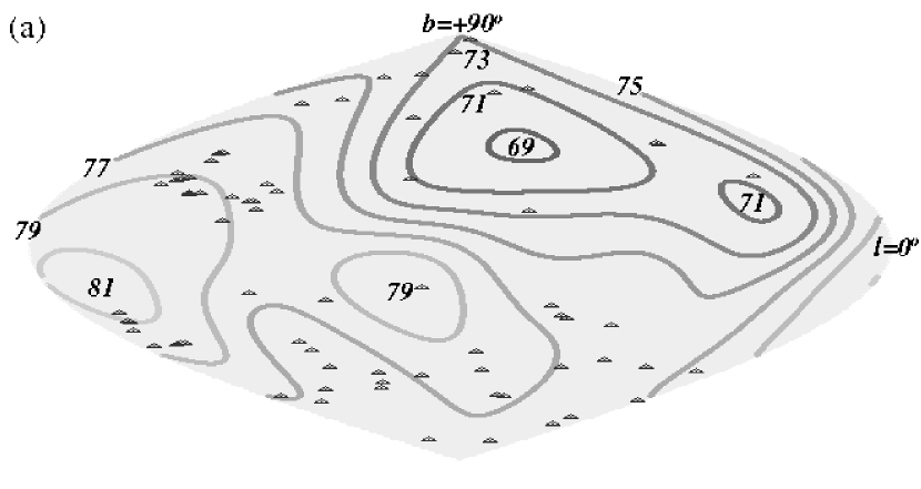
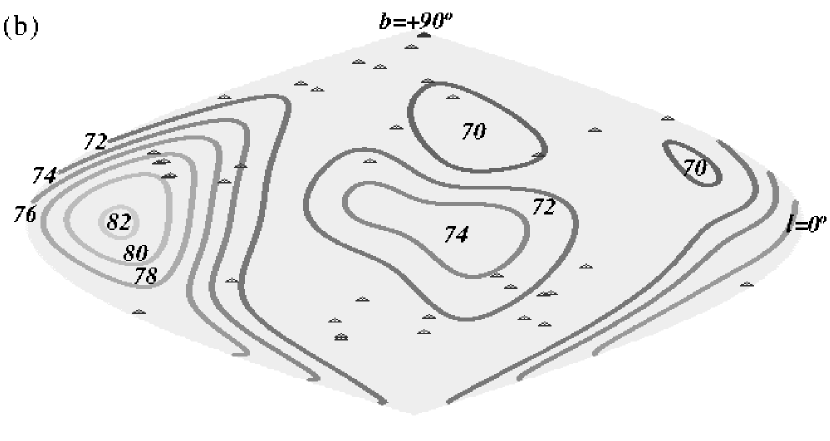
In Fig. 1 contour maps appear (in Galactic co-ordinates) for the HST Key Project data and the comparison data. The extrema are in similar directions for the two data sets and are similar in magnitude, except that one of the maxima in the comparison map is weaker. While the comparison map may not serve as a completely definitive cross-check of the reality of the variations observed in the HST Key Project map, it certainly seems to show some agreement, and it does not differ from the HST Key Project map as much as would be expected if the variation in $H_{0}$ were due to uncertainties in the grid $H_{0}$ values alone. This suggests the variation in the maps exists independently of the uncertainties in the particular determinations of $H_{0}$. Since there is more uncertainty in the comparison map than the Key Project map, the differences between the maps probably mostly reflect errors in the comparison map rather than the Key Project map.

If the Pavo, Pavo 2, and Ursa Major determinations are removed from the HST Key Project data (due to their discrepant values), the map looks largely unchanged from the original: the primary maximum goes down slightly to 80 km s^-1 Mpc^-1 and the primary minimum goes up slightly to 71 km s^-1 Mpc^-1 while the secondary extrema remain the same, so that the secondary extrema now become the primary extrema in this case. If PGC 39724 and NGC 4709 are removed from the comparison data, again the map is largely unchanged: the primary maximum is slightly lower at just under 79 km s^-1 Mpc^-1, while the other extrema appear unchanged. Looking at Fig. 1, it is apparent that the extrema tend not to be centred on the lines-of-sight to the individual data determinations, so the extrema are resulting from trends in the data, rather than from specific high or low $H_{0}$ values.

3.2 Magnitude of variation

As was previously discussed in Sect. 3.1, the Gaussian smearing lessens the range of any real variation. Using Gaussians with successively smaller standard deviations of $20^{\circ}$, $15^{\circ}$, and $10^{\circ}$, as the standard deviation gets smaller, the extrema are picked out with less smearing, but errors in the data also start to have a greater impact. At $10^{\circ}$, the range of variation is greater than 30 km s^-1 Mpc^-1, but the grid values are mostly being determined by individual $H_{0}$ values so the errors in the grid values approach those of the $H_{0}$ determinations. The actual extrema are separated by 38 km s^-1 Mpc^-1, which may be an underestimate to the magnitude of any real variation if the standard deviation could approach zero, but the errors have already become so large that they are likely making the range of variation appear artificially large as it is. Being conservative, the range of variation appears to be $\sim$30 km s^-1 Mpc^-1. Thus, large and small values for the standard deviation yield complementary aspects of the map: smaller standard deviations smooth out the range of variation less, while larger standard deviations yield the overall trend in the map with less error.

One may question whether the variation is statistically significant or whether it is likely that this much variation would be found in the map due to measurement errors in $H_{0}$ alone. Assuming that the 1–$\sigma$ random errors are accurate, the significance of the result can be tested statistically by using Monte Carlo simulations of the data. This is accomplished using two different methods: one which assumes the systematic differences between the mean $H_{0}$ values are real for each of the 4 methods used to derive $H_{0}$, and one which assumes that the systematic differences stem from variations in $H_{0}$ or errors. The first method involves calculating a new value of $H_{0}$ for each position by using the weighted mean value of $H_{0}$ corresponding to the actual distance method that was used to obtain the real $H_{0}$ value, and then adding Gaussian deviates (varied over a 3–$\sigma$ range) to the data using the weighted mean 1–$\sigma$ error for the corresponding method to simulate the expected scatter. The second method involves using the weighted mean value of $H_{0}$ for all the data for the $H_{0}$ value at each position and adding Gaussian deviates to the values according to the actual 1–$\sigma$ errors for each data point.

For 10,000 different sets of simulated data for each Monte Carlo method, $H_{0}$ maps are calculated and the differences between the maximum and minimum $H_{0}$ grid point values are found. Comparing the random sky variations with the observed variations depends strongly on the value of the standard deviation used to smear the values over the sky. This is because smaller standard deviations smooth out the errors less and make it more likely to find greater variation in the maps. For the first method, the results are that the magnitude of variation is only as great as in the real data 5.61% of the time for a standard deviation of $45^{\circ}$ (which yields a range of 6.3 km s^-1 Mpc^-1), 9.90% of the time for a standard deviation of $35^{\circ}$ (which yields a range of 8.8 km s^-1 Mpc^-1), or 37.47% of the time for a standard deviation of $25^{\circ}$ (which yields a range of 12.9 km s^-1 Mpc^-1). The results for the second method are respectively 3.82%, 4.93%, or 13.08%. Thus, assuming the realistic case is somewhere between the two methods, and assuming anything with a less than 5% chance is “statistically significant,” it appears that a statistically significant difference of 6 to 9 km s^-1 Mpc^-1 can be demonstrated with the broader values of the standard deviation.

While the above Monte Carlo methods should give a reasonable measure of the statistical significance of the variation, they depend on the 1–$\sigma$ uncertainties reported for the data being accurate. Independent of the error bars, one can study whether the values are correlated in position on the sky, with higher values tending to be near higher values and lower values tending to be near lower values. Randomly reassigning the $H_{0}$ values to the actual $H_{0}$ positions on the sky and computing maps for several randomizations reveals whether the actual map has more variation than just the scatter in the data should produce. If there is real variation in the data, this method will not yield accurate measures of the statistical significance, since there will be extra scatter in the data that will tend to allow more variation in the map than errors alone should produce. However, this method at least yields an upper limit to the likelihood that as much variation could occur in the map if there were no real variation in the data.

For 10,000 randomizations of the above method, the results are that the range of variation is only as great as for the real map 14.78% of the time for a standard deviation of $45^{\circ}$, 21.55% of the time for a standard deviation of $35^{\circ}$, or 42.10% of the time for a standard deviation of $25^{\circ}$. Thus, even if one is a complete skeptic that there is no real variation in the data, there appears to be more variation than there should be, although of weaker significance than the above Monte Carlo methods found. On the other hand, if there is real variation in the data, these are upper bounds on the percentages, so this weaker significance is not inconsistent with the results of the above methods. Since this method does not depend on uncertainties, it can also be applied to the comparison data. For the complete set of 133 data points, the results are that the variation is only as great 1.16% of the time for a standard deviation of $45^{\circ}$ (which yields a range of 6.6 km s^-1 Mpc^-1), 2.60% of the time for a standard deviation of $35^{\circ}$ (which yields a range of 8.9 km s^-1 Mpc^-1), or 19.29% of the time for a standard deviation of $25^{\circ}$ (which yields a range of 12.6 km s^-1 Mpc^-1). Thus, the difficulty in producing coincidental correlations in larger sets of data allows the conglomerate data set to substantiate a statistically significant variation of $\sim$9 km s^-1 Mpc^-1.

3.3 Directional uncertainty and distance dependence

Figure 2: Hubble constant contour map of Fig. 1(a) with 500 random extrema for maps calculated with Gaussian deviates for the 76 HST Key Project $H_{0}$ values. Positions of the minima and maxima are indicated by dark and light dots respectively, and the contours range from low (dark) to high (light) values of $H_{0}$ (in km s^-1 Mpc^-1) as indicated.

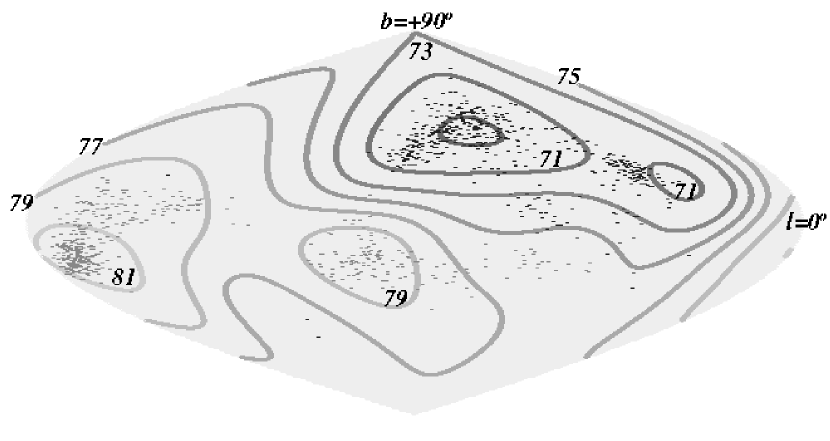
The directional uncertainty of the extrema in the map can be tested by adding Gaussian deviates (in a 3–$\sigma$ range) to the 76 data points, computing the $H_{0}$ grid map, and seeing how much this affects the positions of the maximum and minimum $H_{0}$ grid values in the map. The extrema for each of 500 randomizations are plotted in Fig. 2. Each randomization is calculated with grid separations of $0.5^{\circ}$ so that the extrema can be plotted with less granularity. It can be seen that the probability distribution for the positions of the extrema is not the same in all directions, but primary and secondary extrema exist with directional uncertainties of order $10^{\circ}$ to $20^{\circ}$.

To test the influence of depth on the map, an additional weighting factor for distance is added in the computation of the grid maps. Maps are computed for various nominal distances by weighting the data according to the fraction of the distance that is shared in common with a given nominal distance. For distances more distant than the nominal distance, the weightings go as the ratio of nominal distance to object distance. For distances closer than the nominal distance, the weightings go as the ratio of object distance to nominal distance.

Figure 3: Hubble constant contour maps (in Galactic co-ordinates for a sinusoidal projection of the sky) for the 76 HST Key Project $H_{0}$ values weighted for nominal distances of (a) 30 Mpc, (b) 50 Mpc, (c) 80 Mpc, (d) 120 Mpc, (e) 180 Mpc, and (f) 300 Mpc. Positions of the actual data points are indicated by triangles, and the contours range from low (dark) to high (light) values of $H_{0}$ (in km s^-1 Mpc^-1) as indicated.

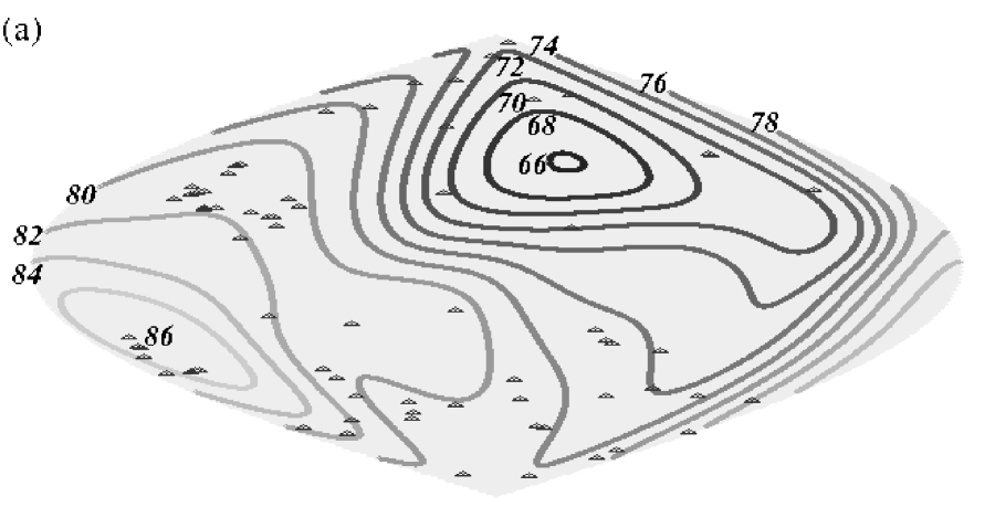
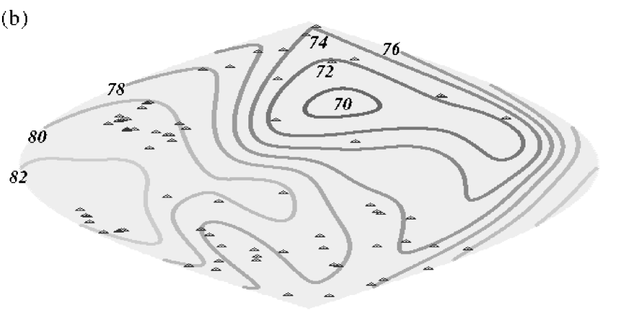
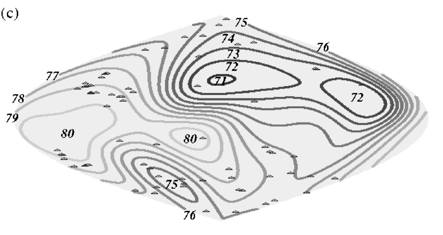
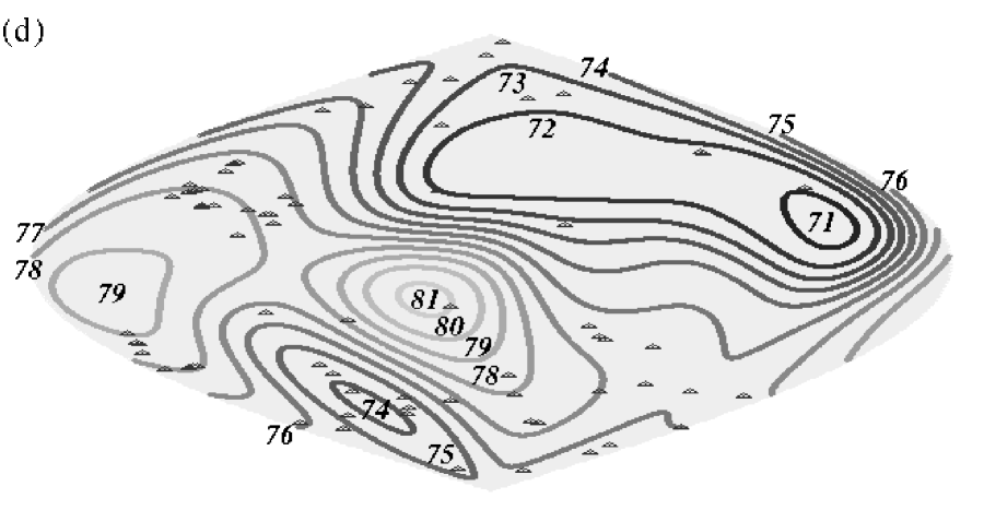
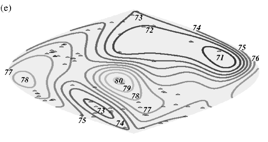
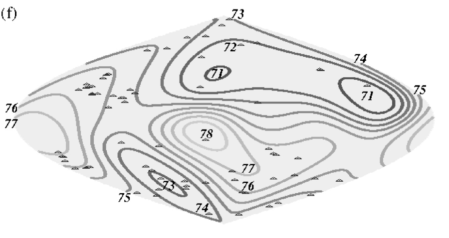
About half of the HST Key Project data are for objects between 13 and 70 Mpc, with the other half between 70 and 467 Mpc. In Fig. 3 distance-weighted maps appear for 6 nominal distances: 30 Mpc, 50 Mpc, 80 Mpc, 120 Mpc, 180 Mpc, and 300 Mpc. It is apparent that nearby, one pair of extrema from Fig. 1 dominates, and the magnitude of variation of this pair falls off with distance. The minimum is near ($\alpha=9^{h}30^{m}$, $\delta=+70^{\circ}$), and the maximum is near ($\alpha=19^{h}30^{m}$, $\delta=-70^{\circ}$). Less apparent is that the grid values of $H_{0}$ at the secondary extrema from Fig. 1 remain roughly constant with distance and dominate only at the greatest distances where the range of variation from the first pair of extrema has become small enough. The secondary minimum is near ($\alpha=18^{h}0^{m}$, $\delta=+15^{\circ}$), and the secondary maximum is near ($\alpha=5^{h}30^{m}$, $\delta=+5^{\circ}$).

It should be noted that more distant values of $H_{0}$ will always sample local expansion as well, and while the converse is not true, the weighting method allows values of $H_{0}$ for the full range of distances to affect all the maps to some degree. The extrema that dominate locally appear to imply some sort of local effect, which could be interpreted as a dipole due to a bulk flow of a local sample volume with respect to the CMB frame, since the extrema are roughly opposite on the sky. The secondary extrema remain constant with distance, and are also roughly opposite of each other on the sky, perhaps suggesting an independent bulk flow of a larger-scale volume.

Removing all the data points from the HST Key Project data set that have an uncertainty greater than 8 km s^-1 Mpc^-1 and producing a map with the remaining 44 points yields a map quite similar to the most distant maps of Fig. 3. The remaining data essentially consist of type Ia supernova measurements and a few other surface brightness fluctuation and fundamental plane measurements that are for distances about 50 Mpc and greater. The map ranges from 68 km s^-1 Mpc^-1 at the minimum to 81 s^-1 Mpc^-1 at the maximum, and the primary extrema of Fig. 1 now appear even weaker than in Fig. 3(f). Since these data mostly have uncertainties of less than 3 km s^-1 Mpc^-1, this provides stronger support for the reality of the extrema observed on large scales in Fig. 3.

It is difficult to make an all-sky map from only 76 points: weighting for distance only makes it more difficult to make meaningful all-sky maps. Thus, to test the significance of the observed variation with distance, the HST Key Project data are combined with the comparison data, and then divided into two sets according to distance. Randomly reassigning the $H_{0}$ values to the data positions for the nearby group of 67 data points (to get a limit on the statistical significance) yields the result that as much variation occurs only 0.16% of the time for a standard deviation of $35^{\circ}$ (which yields a range of variation of 18.8 km s^-1 Mpc^-1) or 7.20% of the time for a standard deviation of $25^{\circ}$ (which yields a range of variation of 25.3 km s^-1 Mpc^-1). Likewise, the more distant group of 66 data points gives respectively 24.39% (corresponding to a range of variation of 6.0 km s^-1 Mpc^-1) or 23.05% (corresponding to a range of 11.1 km s^-1 Mpc^-1). Thus, given that these percentages are upper limits, while the more nearby variation demonstrates that a 19 km s^-1 Mpc^-1 is certainly significant, the more distant variation can not be confirmed to be significant.

Unfortunately, there does not appear to be a reasonable way to use the 1–$\sigma$ errors from the combined data sets to properly determine the statistical significance as in Sect. 3.2, as the errors reported for the comparison data are reported inconsistently and do not share the same systematic errors. However, just using the 36 type Ia supernova values, since they have small random errors and will share systematic errors, and since they tend to be the most distant values, yields interesting results. It is found that as much variation occurs only 0.00% of the time for a standard deviation of $35^{\circ}$ (which yields a range of variation of 6.7 km s^-1 Mpc^-1), 0.02% of the time for a standard deviation of $25^{\circ}$ (which yields a range of variation of 9.7 km s^-1 Mpc^-1), and 0.12% of the time for a standard deviation of $15^{\circ}$ (which yields a range of variation of 12.9 km s^-1 Mpc^-1). If the 1–$\sigma$ errors are truly accurate for the type Ia supernova measurements, it means it is essentially impossible to achieve this much variation by chance. To the extent that these 1–$\sigma$ errors can be trusted, it suggests the variation seen on large scales is statistically significant.

4 Discussion

Figure 4: Hubble constant contour map of Fig. 1(a) transformed to (a) celestial co-ordinates, (b) ecliptic co-ordinates, (c) supergalactic co-ordinates, and (d) the CMB frame. The poles of the CMB frame are defined by the dipole in the CMB in the heliocentric frame, and the longitude right to left is defined such that the North Celestial Pole is at $90^{\circ}$ longitude. Positions of the actual data points are indicated by triangles, and the contours range from low (dark) to high (light) values of $H_{0}$ (in km s^-1 Mpc^-1) as indicated.

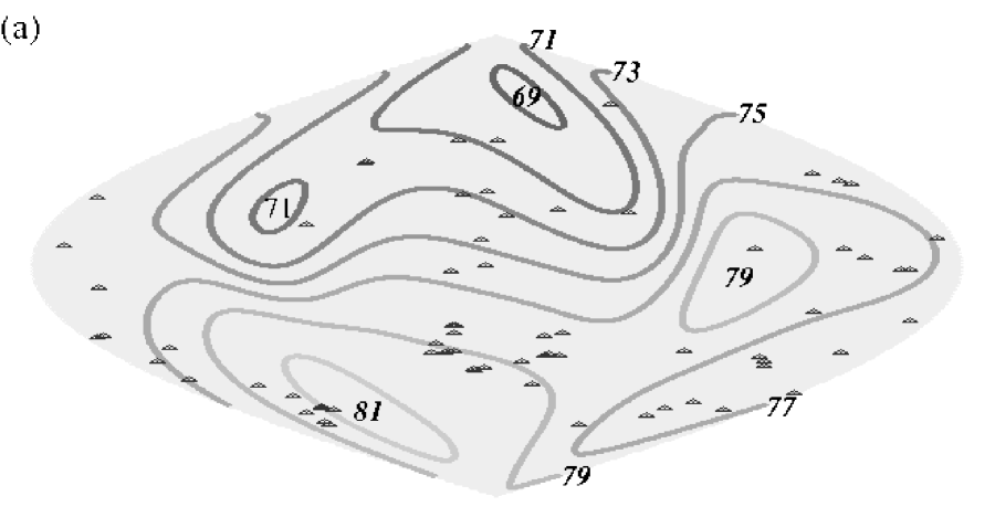
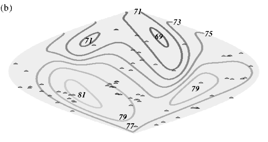
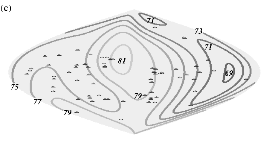
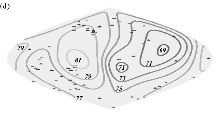
The variation does not appear to be an artifact of Galactic dust, since there is no consistent difference looking in or out of the plane of the Galaxy. In fact, the overall structure in the map is inconsistent with the distribution of dust in the COBE dust maps (Schlegel et al. Sch98, 1998), so it seems unlikely that the observed variation in $H_{0}$ could be due to poor corrections for dust in our own Galaxy. In Fig. 4 the HST Key Project map of Fig. 1(a) has been transformed respectively to celestial co-ordinates, ecliptic co-ordinates, supergalactic co-ordinates, and a CMB-dipole-oriented frame of reference for comparison. Figures 4(a) and 4(b) demonstrate that the extrema do not appear to be an artifact of any local frame of reference.

The supergalactic map is interesting because the extrema that predominate locally are near the supergalactic plane, suggesting they may be associated with local conglomerations of matter (which tend to be arranged along the supergalactic plane). Meanwhile, the extrema that dominate farther out are oriented closer to the supergalactic poles, so if these extrema are a real phenomenon, we may be getting a clear view looking out of the supergalactic plane and observing effects associated with a much larger scale.

The CMB-frame map is oriented with its north pole in the direction of the Sun’s peculiar velocity with respect to the CMB. From the map it is apparent that there is little difference between directions oriented along the CMB dipole. All of the extrema are near the equator of the map, roughly perpendicular to the CMB dipole. Since the $H_{0}$ values have been corrected to be in the CMB frame of reference, this suggests there is no error due to the correction for the CMB dipole: it seems too good in fact. Interestingly, this variation seems to be in agreement with the CMB anisotropy observed by Tegmark et al.Teg03 (2003), who found that the CMB quadrupole and octupole are aligned such that the extrema are in a plane roughly perpendicular to the direction of the dipole. If our dipole motion with respect to the CMB is related to the existence of the $H_{0}$/CMB anisotropy perpendicular to this direction, it suggests this motion and the variations related to it may both be stemming from large-scale inhomogeneities. Inoue and SilkIno06 (2006) have suggested the CMB quadrupole and octupole alignment can be explained by a pair of voids a few hundred Mpc distant in the direction $(l=330^{\circ},b=-30^{\circ})$, which is interestingly in the direction of the $H_{0}$ maxima in our maps.

Figure 5: Hubble constant contour map of Fig. 2 with recent determinations of bulk flows (triangles). From high to low latitude, the bulk flows are those of da Costa et al.daC00 (2000), Dekel et al.Dek99 (1999), WillickWil99 (1999), Hudson et al.Hud04 (2004), Parnovsky et al.Par01 (2001), and Giovanelli et al.Gio98 (1998). Positions of the minima and maxima are indicated by dark and light dots respectively, and the contours range from low (dark) to high (light) values of $H_{0}$ (in km s^-1 Mpc^-1) as indicated.

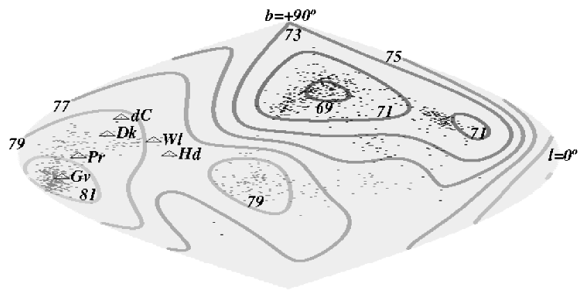
In Fig. 5 recent bulk flow directions are plotted on top of the map of Fig. 2. The bulk flow directions tend to lie on the outskirts of the uncertainty in the maxima, so they are not totally consistent with the map. They should be, as bulk flows will be oriented toward directions associated with higher recessional velocities in the CMB frame and hence the directions of higher $H_{0}$. However, the bulk flow directions do lie in the higher $H_{0}$ regions of the map, so they are not that disconcordant. One thing to note is that the bulk flow directions appear to be sandwiched between the primary and secondary maxima. This suggests that by only looking at the net flow, bulk flow studies may be missing the distinction between two separate effects and missing the actual directions of interest.

5 Conclusion

It appears that a statistically significant variation in $H_{0}$ of at least 9 km s^-1 Mpc^-1 exists in the HST Key Project data. The approximate directional uncertainty is $10^{\circ}$ to $20^{\circ}$. Maps weighted for distance appear to indicate two sets of extrema that dominate on different distance scales. Within our supercluster, differences as great as $\sim$35 km s^-1 Mpc^-1 are observed, and these tend to occur near the supergalactic plane with a minimum near ($\alpha=9^{h}30^{m}$, $\delta=+70^{\circ}$) and a maximum near ($\alpha=19^{h}30^{m}$, $\delta=-70^{\circ}$). Beyond our supercluster, differences as great as $\sim$20 km s^-1 Mpc^-1 are observed, and these tend to occur away from the supergalactic plane with a minimum near ($\alpha=18^{h}0^{m}$, $\delta=+15^{\circ}$) and a maximum near ($\alpha=5^{h}30^{m}$, $\delta=+5^{\circ}$). Within 70 Mpc, a combination of the HST Key Project data and the comparison data shows a statistically significant difference of 19 km s^-1 Mpc^-1. Beyond 50 Mpc, the HST Key Project type Ia supernova data yield a statistically significant difference of 13 km s^-1 Mpc^-1 (assuming the reported 1-$\sigma$ errors are reliable).

Further study of the resilience of this result requires more data specifically selected for achieving optimal sky coverage. It would also be interesting to have data for a greater range of distances to see how far out a statistically significant variation can be detected and over how large a scale the Universe’s expansion needs to be sampled before it appears to become uniform.

Real variation in $H_{0}$ is not really unexpected given the degree of structure and mass inhomogeneity present in the Universe. One implication of this variation is it also partially explains why $H_{0}$ has historically been plagued by so much uncertainty.

We would like to acknowledge useful suggestions and comments from Roberto Abraham, Byron Desnoyers Winmill, John Dubinski, Shoko Sakai, John Tonry, Howard Yee, and the referee. This work was supported by NSERC through a Post-Graduate Scholarship to MLM and a Discovery grant to CCD.

References

- (1) Baum, W. A., Hammergren, M., Thomsen, B., et al., 1997. AJ, 113, 1483.
- (2) Bene, G., Czinner, V., Vasúth, M., 2003. Preprint astro-ph/0308161 v4.
- (3) Bildhauer, S., Futamase, T., 1991. Gen. Relativ. Grav., 23, 1251.
- (4) da Costa, L. N., Bernardi, M., Alonso, M. V., et al., 2000. ApJ, 537, L81.
- (5) Dekel, A., Eldar, A., Kolatt, T., et al., 1999. ApJ, 522, 1.
- (6) Ferrarese, L., Mould, J. R., Kennicutt, R. C., Jr., et al., 2000. ApJ, 529, 745.
- (7) Forbes, D. A., Brodie, J. P., Huchra, J., 1996. AJ, 112, 2448.
- (8) Ford, H. C., Hui, X., Ciardullo, R., Jacoby, G. H., Freeman, K. C., 1996. ApJ, 458, 455.
- (9) Freedman, W. L., Madore, B. F., Gibson, B. K., et al., 2001. ApJ, 553, 47.
- (10) Giovanelli, R., Haynes, M. P., Freudling, W., da Costa, L. N., 1998. ApJ, 505, L91.
- (11) Gregg, M. D., 1997. NewA, 1, 363.
- (12) Herbig, T., Lawrence, C. R., Readhead, A. C. S., Gulkis, S., 1995. ApJ, 449, L5.
- (13) Hjorth, J., Tanvir, N. R., 1997. AJ, 482, 68.
- (14) Hudson, M. J., Smith, R. J., Lucey, J. R., Branchini, E., 2004. MNRAS, 352, 61.
- (15) Inoue, K. T., Silk, J., 2006. ApJ, 648, 23.
- (16) Jensen, J. B., 1997. Ph.D. Thesis, Univ. Hawaii.
- (17) Jensen J. B., Tonry, J. L., Thompson, R. I., et al., 2001. ApJ, 550, 503.
- (18) Kolb, E. W., Matarrese, S., Notari, A., Riotto, A., 2005. Phys. Rev. D, 71, 023524.
- (19) Lauer, T. R., Tonry, J. L., Postman, M., Ajhar, E. A., Holtzman, J. A., 1998. ApJ, 499, 577.
- (20) Liu, M. C., Graham, J. R., 2001. ApJ, 557, L31.
- (21) Madore, B. F., Freedman, W. L., Kennicutt, R. C., et al., 1996. Am. Astron. Soc. Meeting, 189, 108.04.
- (22) Moffat, J. W., Tatarski, D. C., 1995. ApJ, 453, 17.
- (23) Myers, S. T., Baker, J. E., Readhead, A. C. S., Leitch, E. M., Herbig, T., 1997. ApJ, 485, 1.
- (24) Parnovsky, S. L., Kudrya, Y. N., Karachentseva, V. E., Karachentsev, I. D., 2001. Astron. Lett. 27, 765.
- (25) Paturel, G., Lanoix, P., Teerikorpi, P., et al., 1998. A&A, 339, 671.
- (26) Perlmutter, S., Aldering, G., Goldhaber, G., et al., 1999. ApJ, 517, 565.
- (27) Raychaudhuri, A., 1955. Phys. Rev., 98, 1123.
- (28) Russ, H., Soffel, M. H., Kasai, M., Börner, G., 1997. Phys. Rev. D, 56, 2044.
- (29) Sakai, S., Mould, J. R., Hughes, S. M. G., et al., 2000. ApJ, 529, 698.
- (30) Sakai, S., 2001. Private communication.
- (31) Salaris, M., Cassisi, S., 1998. MNRAS, 298, 166.
- (32) Schlegel, D. J., Finkbeiner, D. P., Davis, M., 1998. ApJ, 500, 525.
- (33) Tegmark, M., de Oliveira-Costa, A., Hamilton, A. J., 2003. Phys. Rev. D, 68, 123523.
- (34) Thomsen, B., Baum, W. A., Hammergren, M., Worthey, G., 1997. ApJ, 483, 37.
- (35) Tully, R. B., Pierce, M. J., 2000. ApJ, 533, 744.
- (36) Whitmore, B. C., Sparks, W. B., Lucas, R. A., Macchetto, F. D., Biretta, J. A., 1995. ApJ, 454, L73.
- (37) Willick, J. A., 1999. ApJ, 522, 647.
- (38) Zaroubi, S., 2002. Preprint astro-ph/0206052 v2.
- (39) Zasov, A. V., Bizyaev, D. V., 1996. Astron. Lett., 22, 71.
- (40) Zehavi, I., Riess, A. G., Kirshner, R. P., Dekel, A., 1998. ApJ, 503, 483.