CMB Spectral Distortions from the Scattering of Temperature Anisotropies

Abstract

Thomson scattering of CMBR temperature anisotropies will cause the spectrum of the CMBR to differ from blackbody even when one resolves all anisotropies. A formalism for computing the anisotropic and inhomogeneous spectral distortions of intensity and polarization is derived in terms of Lorentz invariant central moments of the temperature distribution. The formalism is non-perturbative, requiring neither small anisotropies nor small metric or matter inhomogeneities; but it does assume cold electrons. The low order moments are not coupled to the higher order moments allowing one to truncate the equations without any loss of accuracy. This formalism is applied to a standard $\Lambda$-CDM cosmology after reionization where the temperature anisotropies are dominated by the Doppler effect for the bulk motion of the gas with respect to the CMBR frame. The resultant spectral distortion is parameterized by $u\approx 3\times 10^{-8}$, where in this case $u$ is observationally degenerate with the Sunyaev-Zel’dovich (SZ) $y$ parameter. In comparison the expected thermal SZ $y$-distortion from the hot IGM is expected to be $\mathrel{\hbox to0.0pt{\lower 3.0pt\hbox{$\mathchar 536\relax$}\hss}\raise 2.0pt\hbox{$\mathchar 318\relax$}}30$ times larger. However at $z\mathrel{\hbox to0.0pt{\lower 3.0pt\hbox{$\mathchar 536\relax$}\hss}\raise 2.0pt\hbox{$\mathchar 318\relax$}}5$ the effect described here would have been the dominant source of spectral distortions. The effect could be much larger in non-standard cosmologies.

I Introduction

The cosmic microwave background radiation (CMBR) is observed to have a spectrum extremely close to a blackbody (a.k.a. thermal or Planckian) spectrum with temperature $T=2.725\,$K Mather et al. (1994); Wright et al. (1994); Fixsen et al. (1996); Fixsen and Mather (2002). In addition to contamination from foreground radio and far-IR sources, deviations from a thermal spectrum is observed in the direction of concentrations of hot gas (galaxy clusters) due to the thermal Sunyaev-Zel’dovich effect (tSZ) Birkinshaw (1999). If one had better sensitivity one should see some amount of tSZ spectral distortions everywhere since one expect there is ionized gas with $T_{\rm g}\mathrel{\hbox to0.0pt{\lower 3.0pt\hbox{$\mathchar 536\relax$}\hss}\raise 2.0pt\hbox{$\mathchar 318\relax$}}10^{6}$ K along every line-of-sight.

In the Earth frame the brightness temperature of the CMBR is observed to vary by several mK in a dipole pattern; however this would disappear if the observer were boosted into the ”CMBR frame”. After accounting for this velocity dipole there is also observed residual primary anisotropies at the 10s of $\mu$K level concentrated on the sub-degree scales. These anisotropies are expected and observed to be very close to blackbody i.e. the temperature varies with direction on the sky but the spectrum in each direction on the sky is close to a blackbody. If one observes the CMBR with a finite beam instrument, because of the anisotropies, and because the average of a blackbody spectra with different temperature is not a blackbody, the observed spectrum will exhibit a spectral distortion from blackbody Chluba and Sunyaev (2004). This ”beam mixing distortion” is very similar to, and can be confused with, the tSZ distortions mentioned above. However this is not the topic of this paper.

Here the mixing of anisotropic blackbody spectra due to scattering of the radiation is examined. These distortions will occur even with arbitrarily fine angular resolution; and thus are called ”resolved spectral distortions” in contrast to the ”unresolved spectral distortions” from beam mixing. As we shall see, apart from a small and isotropic primordial tSZ effect, the anisotropic blackbody approximation is correct to 1st order in the amplitude of inhomogeneities in the universe, and the resolved distortions caused by coupling of scattering and anisotropies arise in 2nd order. Just from this consideration one can expect the spectral distortion to be very small.

I.1 Roadmap

Here is a brief description of what is included in this paper

§II.1: Temperature transform representation.

§II.2: Decompose transform into moments.

§A: Practical method to compute moments.

§II.3: Central moments shown to be Lorentz invariant.

§II.4: Moments are coefficients in Fokker-Planck expansion.

§II.5: Some properties of expansion.

§II.6: Relation to commonly used power law moments.

§II.7: tSZ $y$-distortion in terms of moments.

§B: Global frames: 3+1 description of space-times.

§III.1: Redshifting of photons in terms of global frame velocity gradients.

§III.2: Thomson cross-section as a convolution.

§III.2: Apply convolution to the temperature transform.

§III.3: Apply convolution to moments.

§IV.1: Spectral distortions are driven by temperature anisotropies.

§IV.2: Cosmological initial conditions and origin of spectral distortions.

§IV.3: Order in cosmological perturbation theory where different terms become non-zero.

§C: Generalizes all of the above to polarized light.

§IV.4: Relates $\bar{T}$ to usual $\Delta T/T$ language.

§IV.5: Lowest order equations for small perturbations.

§IV.6: All moments for small optical depth.

§IV.7: Adds tSZ $y$-distortions.

§V: Application to expected mean spectral distortion.

§D: Details for computing mean distortion.

§VI: Discussion of results.

Many of these sections may be skipped as technical details, depending on your interests.

II Representation of the Spectrum

Usually one quantifies the flux of photons by a brightness $I_{\nu}[{\bf\hat{c}},{\bf x},t]$ where $\nu$, ${\bf x}$, $t$ and ${\bf\hat{c}}$ are respectively the frequency, spatial position, time, and direction in which the photons are traveling (N.B. usually one uses ${\bf\hat{n}}=-{\bf\hat{c}}$). The quantities we will end up dealing with are a highly transformed form of $I_{\nu}$. The first step is to transform to the dimensionless quantum mechanical occupation number $n[\nu,\cdots]\equiv c^{2}I_{\nu}[\cdots]/(4\pi\hbar\nu^{3})$ where $h$ is the Planck constant. Implicit in these definitions is a choice of rest-frame. Of course $\nu$ will be Doppler shifted from one rest-frame to another, but the quantity $n$ is rest-frame independent (i.e. a Lorentz invariant) once one takes into account the Doppler shifting of the argument $\nu$.

Other common representations of the spectra is the brightness temperature, ${T_{\rm b}}$, defined by ${T_{\rm b}}\equiv h\nu/({k_{\rm B}}\,{\rm ln}[1+1/n])$, which gives the temperature of a blackbody which would produce the equivalent brightness at that frequency. Here ${k_{\rm B}}$ is the Boltzmann constant. If $n\gg 1$ this reduce to the Rayleigh-Jeans temperature, ${T_{\rm RJ}}=h\nu\,n/{k_{\rm B}}$. Both ${T_{\rm b}}$ and ${T_{\rm RJ}}$ are frame-dependent.

II.1 The Temperature Transform

A blackbody spectrum has frequency dependence

$$n[\nu,\cdots]={n^{\rm BB}}\left[{h\nu\over{k_{\rm B}}\,T[\cdots]}\right]\qquad{n^{\rm BB}}[x]={1\over e^{x}-1}\ .$$ (1)

where $T$ is the temperature. If for a given ${\bf x}$, $t$, ${\bf\hat{c}}$, the frequency dependence differs from this functional form we say there is a spectral distortion.

Next define the temperature transform Sunyaev and Zel’dovich (1972); Chan and Jones (1975); Salas (1992); Chluba and Sunyaev (2004), $q[{\rm ln}[T]\,\cdots]$, of $n[\nu,\cdots]$, defined implicitly by

$$n[\nu,\cdots]=\int_{-\infty}^{\infty}d{\rm ln}[T]\,q[{\rm ln}[T],\cdots]\,{n^{\rm BB}}\left[{h\nu\over{k_{\rm B}}\,T}\right]\ .$$ (2)

In §2 it is shown that $q[{\rm ln}[T],\cdots]$ is sufficient to represent the spectral distortions that we are interested in here.

II.2 Logarithmic and Central Moments

It is useful to characterize $q[{\rm ln}[T],\cdots]$ by it’s logarithmic moments

$$\eta_{(n)}[\cdots]\equiv\int_{-\infty}^{\infty}d{\rm ln}[T]\,{\rm ln}[T]^{n}\,q[{\rm ln}[T],\cdots]$$ (3)

It is shown how to compute $\eta_{(n)}$ from $n[\nu,\cdots]$ in appendix A. From these moment we will define other parameters beginning with the grayness parameter

$$g\equiv 1-\eta_{(0)}\ .$$ (4)

If $\eta_{(0)}\neq 0$ then $q[{\rm ln}[T],\cdots]/\eta_{(0)}$ integrates to unity and can be thought of as a probability distribution function (pdf) for ${\rm ln}[T]$. Using this pdf one can define the average

$$\langle f[T,\cdots]\rangle\equiv\int_{-\infty}^{\infty}d{\rm ln}[T]\,{q[{\rm ln}[T],\cdots]\over\eta_{(0)}}\,f[T,\cdots]$$ (5)

so that $\eta_{(n)}=\eta_{(0)}\,\langle{\rm ln}[T]^{n}\rangle$. Define the mean logarithmic temperature as

$$\bar{T}\equiv e^{\langle{\rm ln}[T]\rangle}=e^{\eta_{(1)}/\eta_{(0)}},$$ (6)

and the central moments

$$u_{(n)}\equiv\left\langle{\rm ln}\left[{T\over\bar{T}}\right]^{n}\right\rangle=\sum_{k=0}^{n}{(-1)^{k}n!\over k!\,(n-k)!}\,{\eta_{(k)}\over\eta_{(0)}}\,\left({\eta_{(1)}\over\eta_{(0)}}\right)^{n-k}.$$ (7)

Note that by definition $u_{(0)}=1$ and $u_{(1)}=0$. The most important central moment is the 1st non-trivial one, $u_{(2)}$, and for this reason we use the special notation

$$u\equiv u_{(2)}$$ (8)

and give $u$ the name: width of the temperature distribution. A graybody spectrum has $u_{(n)}=0$ for $n>0$ and $g>0$ and this is why $g$ got the name “grayness”.

II.3 Lorentz Transformations

Under a Lorentz transformation, from frame 1 to 2, the various quantities are Doppler shifted

$$\nu_{2} = {\nu_{1}\over 1+z_{12}}$$ (9)

$$\bar{T}_{2} = {\bar{T}_{1}\over 1+z_{12}}$$

$$n_{2}[\nu,\cdots] = n_{1}[(1+z_{12})\,\nu,\cdots]$$

$$q_{2}[{\rm ln}[T],\cdots] = q_{1}[{\rm ln}[T]+{\rm ln}[1+z_{12}],\cdots]$$

The parameters $g$ and $u_{(n)}$ are Lorentz invariant, and this is the main reason why it is convenient to parameterize the spectral distortion by $g$ and the $u_{(n)}$.

II.4 Fokker Planck Expansion

Another reason why the central moments are useful is that the temperature transform of the background radiation spectra will generically give a very narrow distribution of temperature, corresponding to a small overall spectral distortion. That being the case, to the extent that the blackbody spectrum ${n^{\rm BB}}$ is well represented by the Taylor series expansion of it’s argument, $\nu/T$, then the spectral distortion is given by the moments of the temperature distribution. A mnemonic representation of this is to imagine expanding $q$ as a sum of derivatives of Dirac $\delta$-functions centered on some fiducial temperature $T_{0}$, i.e.

$$q[{\rm ln}[T],\cdots]=\sum_{m=0}^{\infty}{(-1)^{m}\over m!}\,d_{(m)}[\cdots]\,{d^{m}\delta\left[{\rm ln}\left[{T\over T_{0}}\right]\right]\over d{\rm ln}[T]^{m}}\ .$$ (10)

Substituting this into the temperature transform one finds, by integrating by parts and assuming ${\rm lim}_{{\rm ln}[T]\rightarrow\pm\infty}q=0$, that

$$n[\nu,\cdots]=\sum_{m=0}^{\infty}{d_{(m)}[\cdots]\over m!}\,\,{\Delta n^{(m)}}\left[{h\nu\over{k_{\rm B}}T_{0}}\right]$$ (11)

where

$${\Delta n^{(m)}}[x]\equiv(-1)^{m}{d^{m}{n^{\rm BB}}[x]\over d{\rm ln}[x]^{m}}\ .$$ (12)

By computing the moments of eq. (10) one can express the coefficients $d_{(m)}$ in terms of $g$, $\bar{T}$, and $u_{(n)}$ and vice versa

$${d_{(m)}\over 1-g} = \sum_{n=0}^{m}{m!\over n!\,(m-n)!}\,{\rm ln}\left[{\bar{T}\over T_{0}}\right]^{m-n}\,u_{(n)}$$ (13)

$$u_{(n)} = \sum_{m=0}^{n}{n!\over m!\,(n-m)!}\,{\rm ln}\left[{T_{0}\over\bar{T}}\right]^{n-m}\,{d_{(m)}\over 1-g}$$

(N.B. $u_{(0)}=1$, $u_{(1)}=0$).

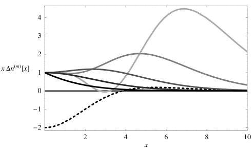
Figure 1: Shown are the spectral perturbation from the lowest order terms in the Fokker-Planck expansion. In particular the thick solid curves show $x\,{\Delta n^{(m)}}[x]$ defined in eq. (12). As one goes from black to gray the thick solid curves correspond to $m=0$ (a graybody distortion), $m=1$ (a temperature or Doppler distortion), $m=2$ (a $u$ distortion), $m=3$, and $m=4$. For reference a $y$-distortion ${\Delta n^{\rm SZ}}[x]=-3{\Delta n^{(1)}}[x]+{\Delta n^{(2)}}[x]$ is shown as a dashed curve. Here $x=h\nu/({k_{\rm B}}T_{0})$ where $T_{0}$ is a temperature which will depend on the context. Note that $x\,\Delta n$ is proportional to the change in Rayleigh-Jeans temperature, $T_{\rm RJ}\equiv(h\nu/{k_{\rm B}})\,n$.

Substituting eq. (II.4) into eq. (11) and using the Taylor series

$${n^{\rm BB}}\left[{h\nu\over{k_{\rm B}}\,\bar{T}}\right]=\sum_{j=0}^{\infty}{(-1)^{j}\over j!}{\rm ln}\left[{\bar{T}\over T_{0}}\right]^{j}{\partial^{j}\over\partial{\rm ln}[\nu]^{j}}{n^{\rm BB}}\left[{h\nu\over{k_{\rm B}}\,T_{0}}\right]$$ (14)

one finds an alternative Fokker Planck series

$$n[\nu,\cdots]=(1-g)\,\sum_{n=0}^{\infty}{u_{(n)}[\cdots]\over n!}\,\,{\Delta n^{(n)}}\left[{h\nu\over{k_{\rm B}}\bar{T}}\right]\ .$$ (15)

Eq. (15) involves the physically defined $\bar{T}$ rather than the arbitrary $T_{0}$ in eq. (11), the later is probably more practically useful since precision spectral measurement are often with respect to a reference blackbody. Of course if $T_{0}=\bar{T}$, then $d_{(m)}=(1-g)\,u_{(m)}$, the two equations are equivalent and $d_{(1)}=0$.

This formalism is most useful when the temperature distribution is narrow enough that the first few terms of these series give an adequate approximation to the spectrum. A truncation of these series at $m\leq N$ we call an order $N$ Fokker-Planck approximation. Strictly speaking a Fokker-Planck approximation corresponds to $N=2$.

II.5 Fokker-Planck Asymptotes

It is easy to compute the asymptotic form of the spectra. A low frequency expansion is

$${\Delta n^{(n)}}[x]=-{1\over 2}+\sum_{p=0}^{\infty}{B_{2p}\over(2p)!}\,(1-2p)^{n}x^{2p-1}$$ (16)

where the $B_{p}$ are the Bernoulli numbers with values $B_{0}=1$, $B_{1}=-{1\over 2}$, while for integer $n\geq 1$: $B_{2n+1}=0$ and $B_{2n}={1\over 2}-\sum_{k=0}^{n-1}{(2n)!B_{2k}\over(2k)!(2(n-k)+1)!}$. A high-frequency expansion is

$${\Delta n^{(n)}}[x]=\sum_{r=1}^{\infty}p_{n}[rx]\,e^{-r\,x}\ .$$ (17)

where the $p_{n}$ are order $n$ polynomials defined by $p_{n}[x]=(-1)^{n}\,e^{x}{d^{n}\over d{\rm ln}[x]^{n}}e^{-x}$ with limiting values ${\rm lim}_{x\rightarrow\infty}p_{n}[x]=x^{n}$ and $p_{n}[0]=\delta_{n,0}$. Both expansions have fairly good convergence properties. From this one sees that ${\rm lim}_{x\rightarrow 0}{\Delta n^{(m)}}[x]=1/x$ and ${\rm lim}_{x\rightarrow\infty}{\Delta n^{(m)}}[x]=x^{m}\,e^{-x}$. The asymptotes are always positive but ${\Delta n^{(m)}}[x]$ will go negative for $n\geq 4$.

II.6 Power Law Moments

The moments $\langle T^{p}\rangle$ are also useful, for example the bolometric brightness is $\propto\langle T^{4}\rangle$ while the number flux of photons is $\propto\langle T^{3}\rangle$. Using eq.s (10,II.4) one finds

$$\langle T^{p}\rangle=T_{0}^{p}\sum_{m=0}^{\infty}{p^{m}\,d_{(m)}\over m!}=(1-g)\,\bar{T}^{p}\sum_{n=0}^{\infty}{p^{n}\,u_{(n)}\over n!}\ .$$ (18)

II.7 Sunyaev Zel’dovich Distortions

While the tSZ effect is not the focus of this paper, it does fit neatly into the formalism just described. The Kompane’ets equation which gives the evolution of spectral distortions due to the tSZ effect, is an $N=2$ Fokker-Planck approximation to the collisional Boltzmann equation with Compton scattering by non-relativistic electrons. A cloud of hot electrons illuminated by a blackbody spectrum with temperature $T_{0}$ will emit photons with a distorted spectrum of the form $n\approx{n^{\rm BB}}\left[x\right]+y\,{\Delta n^{\rm SZ}}\left[x\right]$ where

$${\Delta n^{\rm SZ}}[x] \equiv {x\,e^{x}\over(e^{x}-1)^{2}}\,\left(x\,{e^{x}+1\over e^{x}-1}-4\right)$$

$$= -3{\Delta n^{(1)}}[x]+{\Delta n^{(2)}}[x]$$

which is called a $y$-distortion. Here the “$y$ parameter” is given by a line integral through the gas $y=\int d\tau{k_{\rm B}}({T_{\rm e}}-T_{0})/({m_{\rm e}}c^{2})$ where $\tau=\int c\,{n_{\rm el}}\,{\sigma_{\rm T}}\,dt$ gives the Thomson optical depth, ${\sigma_{\rm T}}=6.65\times 10^{-25}$cm² is the Thomson cross-section, ${n_{\rm el}}$ is the space density of free electrons, and ${k_{\rm B}}{T_{\rm e}}$ is 2/3 of the average kinetic energy of the electrons (so ${T_{\rm e}}$ gives the electron kinetic temperature for a Maxwellian distribution). The validity of eq. (II.7) is $y,\tau\ll 1$ and ${k_{\rm B}}{T_{\rm e}},\,{k_{\rm B}}\,T_{0}\,h\nu\ll{m_{\rm e}}c^{2}$. The latter requirements give the condition for the width of the scattering kernel in frequency space to be narrow, which is the requirement for a Fokker-Planck approximation.

One expects to find a varying $y$-distortion as one scans across the sky, varying according to the density and temperature of hot gas along the lines-of-sight. From eq. (II.7) one sees that

$$g = 1+{\cal O}[y^{2}]$$ (20)

$$\bar{T} = T_{0}\,(1-3\,y+{\cal O}[y^{2}])$$

$$u=u_{(2)} = 2\,y+{\cal O}[y^{2}]$$

$$u_{(n)} = 0+{\cal O}[y^{2}]\quad n\geq 3\ .$$

From eq. (18) one recovers the well known result that the change in the number flux of photons is unchanged: ${\Delta N\over N}=\langle T^{3}\rangle/T_{0}^{3}-1=0$, while the increase of bolometric brightness is ${\Delta E\over E}=\langle T^{4}\rangle/T_{0}^{4}-1=4y$.

Various authors Stebbins (1997a, b); Challinor and Lasenby (1998); Itoh et al. (1998) have examined higher order corrections in ${\Theta_{\rm e}}\equiv{k_{\rm B}}{T_{\rm e}}/({m_{\rm e}}c^{2})$, by expanding the Boltzmann equation in powers of ${\Theta_{\rm e}}$, obtaining expressions like eq. (11) except that the coefficients are powers of ${\Theta_{\rm e}}$. Note that this is only a rearrangement of eq.s (11,15) and the spectral shapes obtained are linear combinations of the ${\Delta n^{(m)}}$. For $\tau,\,h\nu\ll 1$ and a constant temperature gas, one express the spectral distortion by eq. (15) where the $u_{(n)}$ are given by a power series in ${\Theta_{\rm e}}$ beginning with power ${\Theta_{\rm e}}^{n-1}$.

The tSZ effect produces a generic Fokker-Planck distortion, however it can be distinguished from other sources of spectral distortion, even those described by a low order Fokker-Planck expansion. The reason for this is that the tSZ distortions are a one parameter (${\Theta_{\rm e}}$) set of distortions, so that the Fokker-Planck coefficients are not independent but are correlated. From eq. (II.7) one sees that for a pure $y$-distortion (${\cal O}[{\Theta_{\rm e}}^{1}]$), one expects ${\rm ln}[\bar{T}/T_{0}]=-3u_{(2)}/2$. Even if it were contaminated by primordial anisotropies with $u_{(2)}\ll{\rm ln}[\bar{T}/T_{0}]$, one could expect to find the unique tSZ signature:

$${\rm Cov}\left[u_{(2)},{\rm ln}\left[{\bar{T}\over T_{0}}\right]\right]\approx-{3\over 2}\,{\rm Var}[u_{(2)}]$$ (21)

Other sources of distortion will not have this correlation.

III Boltzmann Equation

So far we have just discussed mathematical descriptions of the spectral distortions but not how they arise or their physical dynamics. The equation which describes the evolution of the distribution of photons in phase space (space, time, direction, and frequency) in the presence of scattering is the collisional Boltzmann equation. It can be written as a dynamical equation for the occupation number $n$:

$${D\over Dt}n={d\tau\over dt}C$$ (22)

where $D\over Dt$ is a convective derivative along a null geodesic, $C$ is a dimensionless collision term, and ${d\tau\over dt}$ is the rate of increase of scattering optical depth along the geodesic. This says that $n$ is conserved along trajectories in phase space except for the effects of scattering (which is really the definition of scattering). In an arbitrary space-time the trajectories are given by the geodesic equation, while $C$ and ${d\tau\over dt}$ depends on the type of scattering.

The convective derivative may be written

$${D\over Dt}={\partial\over\partial t}+{d{\bf x}\over dt}\cdot\nabla_{{\bf x}}+{d{\bf\hat{c}}\over dt}\cdot\nabla_{{\bf\hat{c}}}+{d{\rm ln}[\nu]\over dt}{\partial\over\partial{\rm ln}[\nu]}\ .$$ (23)

This equation is purposely written in 3+1, Galilean language, but is applicable in an arbitrary space-time when one chooses a global rest-frame (see appendix B for the specifics). Here ${d{\bf x}\over dt}$ give the flow in position space, while ${d{\bf\hat{c}}\over dt}$ gives the flow in direction space, i.e. the bending of light. These two terms are generally what is known as “lensing”, but in this paper the main interest is in the 4th term, i.e. the flow in frequency space.

III.1 Redshift

In appendix B it is shown that

$${d{\rm ln}[\nu]\over dt}={d{\rm ln}[1+z]\over dt}=-{\bf\hat{c}}\cdot({\bf\nabla}{\bf v})\cdot{\bf\hat{c}}+{\bf\hat{c}}\cdot{\bf a}$$ (24)

where ${\bf\nabla}{\bf v}$ and ${\bf a}$ are respectively the spatial velocity gradient and proper acceleration of the global frame we are using, while $z$ is the redshift ($1+z$ is only defined up to a multiplicative constant).

This is not an expression for redshift which may be familiar to you, but this non-perturbative expression is completely intuitive from well-known, perturbative, Newtonian and cosmological results. The 1st term on the right-hand-side (rhs) gives the line-of-sight component to the velocity gradient of the observer, so this terms can be interpreted as a Doppler redshift having to do with differences in the observers’ velocities. One can interpret $-{\bf a}$ as the gravitational acceleration (${\bf g}=-{\bf a}$ in Newtonian gravity) and the $-{\bf\hat{c}}\cdot{\bf a}$ term gives the gravitational redshift as the photons move against or with the “force of gravity”. In different frames the amount of Doppler and gravitational redshift will differ, but if one considers two fixed endpoints the gravitational redshift plus the correction for the Lorentz boosts between different frames will always agree.

Eq. (24) also produces a non-perturbative expression for “cosmological” space-times. Consider the metric

$$g_{\alpha\beta}={{\rm diag}[-e^{2\phi},e^{-2\psi},e^{-2\psi},e^{-2\psi}]\over(1+{z_{\rm c}}[\eta])^{2}}$$ (25)

where ${z_{\rm c}}[\eta]$ is the cosmological redshift, $\eta$ is the conformal time coordinate, ${\bf x}$ are the spatial coordinates, while $\phi[{\bf x},\eta]$ and $\psi[{\bf x},\eta]$ give arbitrarily large perturbations from a flat Friedman-Robertson-Walker (FRW) space-time (if $\phi=\psi=0$ this would be a flat FRW cosmology). In the coordinate frame, the solution of eq. (24) is

$${1+z_{2}\over 1+z_{1}}={1+{z_{\rm c}}[\eta_{2}]\over 1+{z_{\rm c}}[\eta_{1}]}\,e^{\phi_{1}-\phi_{2}+\int_{\eta_{1}}^{\eta_{2}}d\eta\,(\dot{\phi}+\dot{\psi})}$$ (26)

for the redshift between two points 1 and 2 along any null geodesic, ${\bf r}[\eta]$, in this space-time. Here $\dot{}={\partial\over\partial\eta}$ and $\phi_{i}=\phi[{\bf r}[\eta_{i}],\eta_{i}]$. Note that the logarithm in eq. (24) means that sum of terms on the rhs translate into a product of terms in the expression for $1+z$. Note that if $\phi=\psi=0$ then then the coordinate frame is free-falling, so ${\bf a}=0$, and there is only a Doppler redshift. More generally the Doppler term is divided into two factors: ${1+{z_{\rm c}}[\eta_{2}]\over 1+{z_{\rm c}}[\eta_{1}]}$ and $e^{\int d\eta\,\dot{\psi}}$; the first is known as the cosmological redshift given by the velocity gradient when $\phi=\psi=0$ and the 2nd term arises because when $\dot{\psi}\neq 0$ the coordinates expand or contract leading to additional Doppler shifts for observers moving with the coordinates. The gravitational redshift is also divided into two factors, by splitting ${\bf\hat{c}}\cdot{\bf a}$ into a term which a perfect derivative along the null geodesic and yields $e^{\phi_{1}-\phi_{2}}$ and the remainder which yields $e^{\int d\eta\,\dot{\phi}}$. Mimicing perturbative cosmology terminology one would call $e^{\phi_{1}-\phi_{2}}$ the Sachs-Wolfe (SW) redshift and $e^{int_{\eta_{1}}^{\eta_{2}}d\eta\,(\dot{\phi}+\dot{\psi})}$ the integrated Sachs-Wolfe (ISW) redshift. These expressions are remarkably similar to the well-known result for linear perturbations; even though this is completely non-perturbative. Of course eq. (25) does not include the most general perturbations from a flat FRW space-time (i.e. no vector or tensor perturbations), and one still has to solve for the trajectory ${\bf r}[\eta]$ first.

III.2 Thomson Scattering in the Baryon Frame

Now since we are using a particular global frame in which to write the Boltzmann equation, it is most convenient to use the baryon frame in which the electrons are at rest. An important point here is that we are considering only the spectral distortion for a cold gas of electrons, and specifically ignoring the electron velocity dispersion, which will also produce a spectral distortion via the tSZ effect. In some, but not all cases, the tSZ effect will dominate the spectral distortion considered here, but as the anisotropy-scattering coupling considered here has usually been neglected it is worthwhile to consider it on it’s own.

Here we consider not only cold electrons but also the limit of low energy photons i.e. $h\nu\ll{m_{\rm e}}c^{2}$. In this case the cross-section for scattering an unpolarized beam is proportional to

$$\Sigma[{\bf\hat{c}},{\bf\hat{c}}^{\prime}]={3\over 16\pi}\left(1+({\bf\hat{c}}\cdot{\bf\hat{c}}^{\prime})^{2}\right)$$ (27)

Using the the notation

$${\hat{\Sigma}\star}F[a,b^{\prime}]\equiv\int d^{2}{\bf\hat{c}}^{\prime}\,\Sigma[{\bf\hat{c}},{\bf\hat{c}}^{\prime}]\,F[a[{\bf\hat{c}}],b[{\bf\hat{c}}^{\prime}]]\ .$$ (28)

the Boltzmann eq. (22) becomes

$${D\over Dt}n={d\tau\over dt}\,{\hat{\Sigma}\star}(n^{\prime}-n).$$ (29)

Henceforth a ^′’d quantity indicates that it is evaluated at direction ${\bf\hat{c}}^{\prime}$. Note that ${\hat{\Sigma}\star}$ is a linear convolution operator since ${\hat{\Sigma}\star}1=1$.

III.3 Temperature Transform of Boltzmann Equation

Substituting eq. (2) into eq. (29) one finds that the Boltzmann equation for $q[{\rm ln}[T],{\bf\hat{c}},{\bf x},t]$ in the baryon frame is

$${Dq\over Dt}={d\tau\over dt}\,{\hat{\Sigma}\star}\,(q^{\prime}-q)$$ (30)

where the convective derivative in temperature space is

$${D\over Dt}={\partial\over\partial t}+{d{\bf\hat{c}}\over dt}\cdot\nabla_{\bf x}+{d{\bf\hat{c}}\over dt}\cdot\nabla_{\bf\hat{c}}+{d{\rm ln}[1+z]\over dt}{\partial\over\partial{\rm ln}[T]}\ .$$ (31)

III.4 Boltzmann Equation of Moments

When one deal with temperature moments the temperature dependence is already “removed” so in what follows we use the convective derivative

$${{\cal D}\over{\cal D}t}={\partial\over\partial t}+{d{\bf x}\over dt}\cdot\nabla_{\bf x}+{d{\bf\hat{c}}\over dt}\cdot\nabla_{\bf\hat{c}}$$ (32)

and any effect of redshifting is shifted to the rhs of the equation. Since $g$ and $u_{(n)}$ are Lorentz invariant there will be no redshifting terms for these quantities. With this convention if we substitute eq. (3) into eq. (30) then we find

$${{\cal D}\eta_{(n)}\over{\cal D}t}=n\,{d{\rm ln}[1+z]\over dt}\,\eta_{(n-1)}+{d\tau\over dt}\,{\hat{\Sigma}\star}(\eta_{(n)}^{\prime}-\eta_{(n)})\ .$$ (33)

This equation tells us that the $\eta_{(n)}$ moments depend only on moments with smaller $n$ so that one may without loss of accuracy truncate the evolution of the moments at any order $n$.

What one really wants is the evolution of $g$, $\bar{T}$, the central moments $u_{(n)}$; which one obtains by combining eq.s (4,6,7) with eq. (33) to obtain

$${{\cal D}g\over{\cal D}t} = {d\tau\over dt}\,{\hat{\Sigma}\star}(g^{\prime}-g)$$

$${{\cal D}{\rm ln}[{\bar{T}\over 1+z}]\over{\cal D}t} = {d\tau\over dt}\,{\hat{\Sigma}\star}\left({1-g^{\prime}\over 1-g}\,{\rm ln}\left[{\bar{T}^{\prime}\over\bar{T}}\right]\right)$$

$${{\cal D}u_{(n)}\over{\cal D}t} = {d\tau\over dt}\,{\hat{\Sigma}\star}\left({1-g^{\prime}\over 1-g}\,U_{(n)}\right)$$

$$U_{(n)} = \left(\sum_{m=0}^{n}{n!\over m!(n-m)!}\,{\rm ln}\left[{\bar{T}^{\prime}\over\bar{T}}\right]^{n-m}\,u_{(m)}^{\prime}\right)$$ (34)

$$-n\,{\rm ln}\left[{\bar{T}^{\prime}\over\bar{T}}\right]\,u_{(n-1)}-u_{(n)}$$

Eq.s (III.4), along with the polarized version, eq.s (147), are the main results of this paper.

As with the $\eta_{(n)}$ this set of coupled equations can be truncated at any order $N$, leading to an accurate representation of all the spectral components ${\Delta n^{(n)}}$ up to order $N$. Of course a truncation does not give a complete description of the spectrum. Note that this is not a perturbation expansion, rather these are completely non-perturbative equations for arbitrary space-times and for large spectral distortions. The assumptions are cold electrons ${k_{\rm B}}{T_{\rm e}}\ll{m_{\rm e}}c^{2}$, soft photons $h\nu\ll{m_{\rm e}}c^{2}$, only Thomson scattering, and unpolarized light. All of these assumptions are liable to be real limitations in applicability. The lack of polarization in these equations was done for simplicity, the formulae including polarization is given in appendix C. In most applications polarization will lead only to a small correction and in some cases polarization is completely negligible. These equations are tied to the gas frame which may not be most convenient for every application. It is relatively simple to translate these equations into a different frame: note that $g$ and $u_{(n)}$ are frame invariant while $t$, ${\bf\hat{c}}$, $\bar{T}$ and all the dot products are not.

III.4.1 Boltzmann Equation for $u$

As we shall see the most important distortions are the lowest order ones, i.e. $g$, $\bar{T}$ and $u=u_{(2)}$. The equations for $g$ and $u$ are explicit in eq.s (III.4) and here is the explicit equation for $u=u_{(2)}$:

$${{\cal D}u\over{\cal D}t}={d\tau\over dt}\,{\hat{\Sigma}\star}\left({1-g^{\prime}\over 1-g}\,\left((u^{\prime}-u)+{\rm ln}\left[{\bar{T}^{\prime}\over\bar{T}}\right]^{2}\right)\right)\ .$$ (35)

One sees that apart from convection, the $u$ distortion is sourced by spectral anisotropy, $u^{\prime}-u$, and by temperature anisotropy ${\rm ln}[\bar{T}^{\prime}/T]$. This is illustrative of all the moments moments $u_{(n)}$ in that ${\rm ln}[\bar{T}^{\prime}/\bar{T}]$ can directly produce $u_{(n)}$ and in that the equation is linear in $u_{(n)}$. For $n>2$ the scattering term is more complicated and always includes non-linear coupling between ${\rm ln}[\bar{T}^{\prime}/\bar{T}]$ and $u_{(m)}$.

IV Spectral Dynamics

IV.1 Temperature and Spectral Anisotropies

Here the word anisotropy is used to mean any function of the $n[\nu,{\bf\hat{c}},\cdots]$ at which is zero when $n$ is independent of ${\bf\hat{c}}$. This includes functions of $q$, $\eta_{(n)}$, $g$, $\bar{T}$, or $u_{(m)}$ which are zero when there is no ${\bf\hat{c}}$ dependence. It is clear for eq.s (30,33) that the collision term in the Boltzmann equation is an anisotropy. One can also see this most clearly for eq. (III.4) by grouping the $u_{(m)}$ dependence of $U_{(n)}$, i.e. decomposing $U_{(n)}=\sum_{m=0}^{n}U_{(n,m)}$ where

$$U_{(n,0)}\hskip-8.0pt = \hskip-8.0pt{\rm ln}\left[{\bar{T}^{\prime}\over\bar{T}}\right]^{n}$$ (36)

$$U_{(n,1)}\hskip-8.0pt = \hskip-8.0pt0$$

$$U_{(n,n)}\hskip-8.0pt = \hskip-8.0ptu_{(n)}^{\prime}-u_{(n)}$$

$$U_{(n,n-1)}\hskip-8.0pt = \hskip-8.0ptn\,{\rm ln}\left[{\bar{T}^{\prime}\over\bar{T}}\right]^{n-m}\,(u_{(n-1)}^{\prime}-u_{(n-1)})\hskip 11.0ptn\geq 3$$

$$\tilde{U}_{(m,n)}\hskip-8.0pt = \hskip-8.0pt{n!\over m!\,(n-m)!}{\rm ln}\left[{\bar{T}^{\prime}\over\bar{T}}\right]^{n-m}u_{(m)}^{\prime}\hskip 5.0pt{n\geq 3\atop m\in[2,n-2]}\ .$$

In eq.s (III.4,IV.1) contains terms like ${\rm ln}\left[\bar{T}^{\prime}\over\bar{T}\right]$, which is a temperature anisotropies and terms like $g-g^{\prime}$, and $u_{(n)}^{\prime}-u_{(n)}$ which are spectral anisotropies. Note again that if the spectral and temperature anisotropies are zero then the scattering term is zero.

IV.2 Initial Conditions and Origin of Spectral Distortions

At very early times electron and atomic scattering is sufficient to nearly completely isotropize and thermalize the photon distribution to an isotropic blackbody, so the initial conditions (ICs) are

$${\rm lim}_{t\rightarrow 0}\{g,\,{\rm ln}\left[{\bar{T}^{\prime}\over\bar{T}}\right],\,u_{(n>0)}\}=0\ .$$ (37)

So the spectral distortions evolve from zero and the reason they exist is because of inhomogeneities. Starting with these ICs one sees from eq. (III.4) that

$$g=0\ .$$ (38)

Note however that this result does not take into account other radiative foreground which can cause $g$ to vary from zero.

The initial growth of temperature anisotropy is given by

$${\rm lim}_{t\rightarrow 0}{\partial{\rm ln}\left[{\bar{T}[{\bf\hat{c}}_{2},\cdots]\over\bar{T}[{\bf\hat{c}}_{1},\cdots]}\right]\over\partial t} = {d{\rm ln}\left[{1+z[{\bf\hat{c}}_{2},\cdots]\over 1+z[{\bf\hat{c}}_{1},\cdots]}\right]\over dt}$$ (40)

$$\hskip-125.0pt=({\bf\hat{c}}_{2}-{\bf\hat{c}}_{1})\cdot{\bf a}_{\rm p}+{\bf\hat{c}}_{1}\cdot(\nabla{\bf v})\cdot{\bf\hat{c}}_{1}-{\bf\hat{c}}_{2}\cdot(\nabla{\bf v})\cdot{\bf\hat{c}}_{2}\ .$$

Thus anisotropies in the baryon frame are initially caused by acceleration of the gas (${\bf a}_{\rm p}\neq 0$ usually due to pressure gradients) and/or by anisotropic gas velocity gradients (shear). Shear will always be a consequence of inhomogeneities in the universe and will inevitably lead to temperature anisotropies. One sees from eq.s (III.4) that anisotropy will lead to time varying, and hence nonzero, spectral distortions $u_{(n)}$. Note however that scattering tends to damp existing temperature anisotropies toward zero so the amount of anisotropy and associated spectral distortions are highly suppressed until scattering turns off at recombination.

IV.3 Perturbative Analysis

Consider a one parameter family of solutions to the full equations-of-motion (EoMs) for matter and gravity as well as the initial conditions (ICs). When $\epsilon=0$ the EoMs and ICs give the unperturbed background cosmology, and more generally $\epsilon$ gives the amplitude of the perturbation from the background solution. One can Taylor series the EoMs and ICs about $\epsilon=0$ and then solve them at each order using the lower order solutions. The ICs may be stochastic. One can Taylor series in $\epsilon$ about 0 any quantity which depends on the solution, e.g. $Q=\sum_{p=0}^{\infty}Q^{\{i\}}\epsilon^{p}$ If the smallest $p$ for which the $Q^{\{n\}}\neq 0$ is $N$ then one says that $Q$ is a perturbation variable of order $N$ and denote this by $Q\sim{\cal O}[N]$. For two quantities $P$ and $Q$, if $P-Q\sim{\cal O}[N]$ then one sees that $P^{\{M\}}=Q^{\{M\}}$ for all $M<N$.

The solution of our EoMs, eq. (38), tells us that $g\sim{\cal O}[\infty]$ although, as mentioned above, additional radiative processes will cause a non-zero $g$ at some order. Since an unperturbed cosmology is by definition homogeneous and everywhere isotropic one must have

$${\rm ln}\left[{\bar{T}^{\prime}\over\bar{T}}\right]^{\{0\}}=(\nabla_{\bf x}n)^{\{0\}}=(\nabla_{\bf\hat{c}}n)^{\{0\}}={d{\bf\hat{c}}\over dt}^{\{0\}}=0\ .$$ (41)

We know from §IV.2 that ${\rm ln}\left[{1+z[{\bf\hat{c}}_{2},\cdots]\over 1+z[{\bf\hat{c}}_{1},\cdots]}\right]\sim{\cal O}[1]$ and hence ${\rm ln}[\bar{T}^{\prime}/\bar{T}]\sim{\cal O}[1]$. It follows that ${\rm ln}[\bar{T}^{\prime}/\bar{T}]^{n}\sim{\cal O}[n]$ and given the ICs of eq. (37) one can see from eq.s (III.4) that $u_{(n)}\sim{\cal O}[n]$ for $n\geq 2$ (by definition $u_{(0)}=1\sim{\cal O}[0]$ and $u_{(1)}=0\sim{\cal O}[\infty]$). Thus for perturbation theory at a given order $N$ one need only consider $u_{(n)}$ for $n\leq N$. In linear theory, $N=1$, there is no spectral distortion, only temperature anisotropy. From the scattering of anisotropies the lowest order spectral distortion is $u=u_{(2)}\sim{\cal O}[2]$, i.e. spectral distortions only appear in 2nd order perturbation theory.

These conclusions depend on our EoMs which ignore certain radiative processes. In particular only non-relativistic Thomson scattering with $h\nu\,{k_{\rm B}}T_{\rm e}\ll m_{\rm e}\,c^{2}$ has been assumed. Finite temperature and frequency corrections are small, but so are the spectral distortions. Long before recombination these conditions are violated but the scattering tends to damp spectral distortions and I estimate these corrections are relatively small although formally they do decrease the order of the spectral distortions. Even at ${\cal O}[0]$ there will be finite temperature differences between the electrons and photons which will lead to a 0th order isotropic spectral distortion from the tSZ effect, i.e. the isotropic part of $\langle u_{(n)}\rangle_{{\bf\hat{c}}}\sim{\cal O}[0]$, an effect not included in our EoMs. However the amplitude of these terms does decrease rapidly with $n$ because it is non-relativistic tSZ. Furthermore even $\langle u_{(2)}\rangle_{{\bf\hat{c}}}$ is very small. Spectral anisotropies from this effect only arise through coupling to temperature anisotropies, so the formally anisotropic part, is of higher order $u_{(n)}-\langle u_{(n)}\rangle_{{\bf\hat{c}}}\sim{\cal O}[1]$, although this again is a small effect and decreases rapidly with $n$.

The most important spectral distortion which has been ignored, is from tSZ at low $z$ caused by shock-heated gas. Shock heating is, arguably, a non-perturbative process, but nevertheless may lead to the largest spectral distortion.

IV.4 ${\Delta T\over T}$

One normally denotes a temperature anisotropy by $\Delta T/T$. What this specifically means may vary, but in many cases ${\Delta T\over T}=({T_{\rm b}}-T_{0})/T_{0}$ where $T_{0}$ is some reference temperature and ${T_{\rm b}}$ is the brightness temperature at a particular frequency. If $g=u_{(n)}=0$ but $\bar{T}\neq 0$ then from eq.s (11-II.4) the distorted spectrum is

$$n={1\over e^{x}-1}\,\left(1+{\rm ln}\left[{\bar{T}\over T_{0}}\right]\,{x\,e^{x}\over e^{x}-1}\right)\qquad x={h\nu\over{k_{\rm B}}T_{0}}\ .$$ (42)

If one Taylor expands the dependence of ${T_{\rm b}}$ on ${\rm ln}[\bar{T}/T_{0}]$ about 0 one finds

$${\Delta T\over T} \equiv {{T_{\rm b}}-T_{0}\over T_{0}}={\rm ln}\left[{\bar{T}\over T_{0}}\right]$$

$$\hskip-30.0pt+\left(1-{x\over 2}+{x\over e^{x}-1}\right)\,{\rm ln}\left[{\bar{T}\over T_{0}}\right]^{2}+{\cal O}\left[{\rm ln}\left[{\bar{T}\over T_{0}}\right]^{3}\right]\ .$$

Of course $\bar{T}\sim{\cal O}[0]$ and by the assumed symmetry $\bar{T}^{\{0\}}={T_{\rm c}}[t]$ which is independent of ${\bf x}$ and ${\bf\hat{c}}$. It then follows that $(\Delta T/T)^{\{1\}}={\rm ln}[\bar{T}/{T_{\rm c}}[t]]^{\{1\}}$ and

$${\rm ln}\left[{\bar{T}^{\prime}\over\bar{T}}\right]^{\{1\}}={{\Delta T\over T}^{\prime}}^{\{1\}}-{\Delta T\over T}^{\{1\}}\ .$$ (44)

i.e. for small anisotropies ${\rm ln}[\bar{T}^{\prime}/\bar{T}]$ reduces to the conventional definition of temperature anisotropy!

IV.5 Lowest Order Spectral Distortions

Given homogeneity and isotropy of the background solution and using ${d{\rm ln}[1+z]\over dt}^{\{0\}}=-H[t]$ where $H$ is the Hubble parameter, the only non-trivial part of 0th order Boltzmann equations is

$${d{\rm ln}[{T_{\rm c}}[t]]\over dt}=-H[t]\ .$$ (45)

Defining the cosmological redshift ${z_{\rm c}}[t]=-1+e^{\int_{t}^{t_{0}}\,dt^{\prime}\,H[t^{\prime}]}$, the solution is the usual temperature-redshift relation ${T_{\rm c}}[t]={T_{\rm c}}[t_{0}]/(1+{z_{\rm c}}[t])$.

The only non-trivial 1st order equation is the usual linearized Boltzmann equation for ${\Delta T\over T}$ in a frame comoving with the baryons. This is what is usually used to calculate CMBR anisotropies. What is new here only enters at $\sim{\cal O}[2]$, which is where the lowest order spectral distortion arise. These lowest order distortion are solutions to the 2nd order equations for $u=u_{(2)}$:

$$\hskip-20.0pt{\partial u^{\{2\}}\over\partial t}+\left({d{\bf x}\over dt}\cdot\nabla_{\bf x}\right)^{\{0\}}u^{\{2\}}+\left({d{\bf\hat{c}}\over dt}\cdot\nabla_{\bf\hat{c}}\right)^{\{0\}}u^{\{2\}}$$ (46)

$$\hskip-20.0pt={d\tau\over dt}^{\{0\}}\,{\hat{\Sigma}\star}\left(u^{\prime\{2\}}-u^{\{2\}}+\left({{\Delta T\over T}^{\{1\}}}^{\prime}-{\Delta T\over T}^{\{1\}}\right)^{2}\right)$$

The 0th order gradient operators depends on the coordinate system one uses in the background cosmology, but if one is perturbing from a flat, $\Omega_{0}=1$, universe then one can choose comoving Euclidean coordinates normalized to ${z_{\rm c}}=0$ so that $d{\bf\hat{c}}/dt^{\{0\}}=0$ and $\left((d{\bf x}/dt)\cdot\nabla_{\bf x}\right)^{\{0\}}=c\,(1+{z_{\rm c}}[t])\,{\bf\hat{c}}\cdot\nabla_{\rm co}$. Eq. (46) is derived in the frame comoving with the baryons. In 1st order perturbation theory, to transform to another frame only involves correcting the dipole component of temperature anisotropy for the Doppler shift caused by the velocity of the baryons in the new frame, since angles are not changed to 1st order and $u$ is frame independent.

Thus in an arbitrary frame (i.e. gauge) to 1st order make the substitution

$${\Delta T\over T}^{\{1\}}[{\bf\hat{c}},{\bf x},t]={\Delta T\over T}^{\{1\}}[{\bf\hat{c}},{\bf x},t]\biggl{|}_{\rm baryon\atop frame}-{{\bf\hat{c}}\cdot{\bf v}_{\rm b}^{\{1\}\over c}}$$ (47)

where ${\bf v}_{\rm b}$ is the baryon velocity in the new frame. The lowest order equation for $u$ in the new frame is thus

$$\hskip-20.0pt{\partial u\over\partial t}+c\,(1+{z_{\rm c}})\,{\bf\hat{c}}\cdot\nabla_{\rm co}\,u$$ (48)

$$\hskip-20.0pt={d\overline{\tau}\over dt}{\hat{\Sigma}\star}\left(u^{\prime}-u+\left({\Delta T\over T}^{\prime}-{\Delta T\over T}+{({\bf\hat{c}}-{\bf\hat{c}}^{\prime})\cdot{\bf v}_{\rm b}\over c^{2}}\right)^{2}\right)$$

where the order superscripts have been dropped, and $\overline{\tau}$ is used for the 0th order optical depth, to emphasize that it is spatially constant. This equation is sufficient for most applications, since the anisotropies are small, the spectral distortions are even smaller, and the lowest order spectral distortion will be, by far, the largest.

IV.6 Single Scattering

A commonly used approximation where the optical depth to scattering is small, for example in the modeling of tSZ effect for clusters of galaxies, is to assume the photons undergo at most one scattering, and that the light incident on gas is isotropic, unpolarized, and spectrally undistorted. Here allow the incident light to have anisotropic $\bar{T}$ but zero $g$ and $u_{(n)}$ (for $n\geq 1$). Under these assumption most of the terms in eq.s (III.4) are zero and one can express the solution as an integral along the photon trajectory:

$$u_{(n)}=\int d\tau\,{\hat{\Sigma}\star}{\rm ln}\left[{\bar{T}^{\prime}\over\bar{T}}\right]^{n}\ .$$

The polarized version of this integral comes by substituting $g=0$ and $\vbox{\halign{$#$\cr{\leftarrow}\mkern-6.0mu\cleaders\hbox{${\bf U}$}\hfill\mkern-6.0mu{\to}\cr\kern-1.00148pt\nointerlineskip\cr\hfil{\bf U}\hfil\cr}}_{(n)}=\delta_{n,0}\vbox{\halign{$#$\cr{\leftarrow}\mkern-6.0mu\cleaders\hbox{${\bf I}$}\hfill\mkern-6.0mu{\to}\cr\kern-1.00148pt\nointerlineskip\cr\hfil{\bf I}\hfil\cr}}/2$ into eq.s (147,174) and integrating to obtain

$$\vbox{\halign{$#$\cr{\leftarrow}\mkern-6.0mu\cleaders\hbox{${\bf U}$}\hfill\mkern-6.0mu{\to}\cr\kern-1.00148pt\nointerlineskip\cr\hfil{\bf U}\hfil\cr}}_{(n)}={3\over 4}\int d\tau\,{\left\langle{\rm ln}\left[{\bar{T}^{\prime}\over\bar{T}}\right]^{n}\vbox{\halign{$#$\cr{\leftarrow}\mkern-6.0mu\cleaders\hbox{${\bf I}$}\hfill\mkern-6.0mu{\to}\cr\kern-1.00148pt\nointerlineskip\cr\hfil{\bf I}\hfil\cr}}\hskip-2.0pt\cdot\hskip-2.0pt\vbox{\halign{$#$\cr{\leftarrow}\mkern-6.0mu\cleaders\hbox{${\bf I}$}\hfill\mkern-6.0mu{\to}\cr\kern-1.00148pt\nointerlineskip\cr\hfil{\bf I}\hfil\cr}}^{\prime}\hskip-2.0pt\cdot\hskip-2.0pt\vbox{\halign{$#$\cr{\leftarrow}\mkern-6.0mu\cleaders\hbox{${\bf I}$}\hfill\mkern-6.0mu{\to}\cr\kern-1.00148pt\nointerlineskip\cr\hfil{\bf I}\hfil\cr}}\right\rangle_{{\bf\hat{c}}^{\prime}}}\ .$$ (49)

The trace of this is eq. (IV.6). Both of these integrals can give a good approximation to all of the moments in some situations.

IV.7 Adding Thermal SZ

Much of the formalism developed in this paper is appropriate for arbitrarily large spectra distortions but restricted to cold electrons. The tSZ effect described in §II.7 will provide a correction to the collision term of the Boltzmann equation due to finite velocity dispersion of the electrons. This effect is most well known for the case of small spectral distortions and non-relativistic electron velocity dispersions in which case one gets a $y$-distortion. In this small distortion limit one can simply add the $y$ distortion as a collision term in addition to the Thomson scattering term already included. To do this one need only note the the relation of $y$ to the central moments given in eq. (20). We see that there is no modification needed for the Boltzmann equation of $g$ and $u_{(n)}$ for $n\geq 3$. The only modifications are for $\bar{T}$ and $u=u_{(2)}$, which in the baryon frame are then corrected by

$${{\cal D}{\rm ln}[{\bar{T}\over 1+z}]\over{\cal D}t} = \cdots-3\,{dy\over dt}$$ (50)

$${{\cal D}u\over{\cal D}t} = \cdots+{dy\over dt}$$

The validity of this equation is only for small distortions so one should restrict oneself to lowest order terms as in eq. (48). The usual expression for the total $y$ along a trajectory is $y=\int dt\,(d\tau/dt)\,{k_{\rm B}}\,({T_{\rm e}}-T_{\gamma})/({m_{\rm e}}c^{2})$ where $\tau$ is the Thomson optical depth used previously, ${T_{\rm e}}$ is the electron temperature, and $T_{\gamma}$ is the photon temperature assumed nearly thermal and isotropic. More generally, when the electrons are non-relativistic but isotropic, one can use ${k_{\rm B}}{T_{\rm e}}={1\over 3}{m_{\rm e}}\overline{{v_{\rm e}}^{2}}$, where $\overline{v_{\rm e}^{2}}$ is the velocity dispersion of the electrons. For $T_{\gamma}$ one wants the average temperature of the photons scattered into the beam so one should use $T_{\gamma}={\hat{\Sigma}\star}\bar{T}^{\prime}$. Thus one should use

$${dy\over dt}={d\tau\over dt}\,{{k_{\rm B}}\,{\hat{\Sigma}\star}({T_{\rm e}}-\bar{T}^{\prime})\over{m_{\rm e}}c^{2}}\ .$$ (51)

One should expect similarities between the tSZ effect and the scattering of anisotropies. This is because underlying both is non-relativistic Compton scattering i.e. Thomson scattering. The relativistic corrections to the Thomson cross-section in the center-of-mass frame only enters when the center-of-mass kinetic energy $KE_{\rm cm}$ approaches ${m_{\rm e}}c^{2}$. For microwave photons this would require electron energies of several TeV. For lower energies the tSZ effect is just the sum of Thomson scatterings with varying Lorentz boosts depending on the motion of the electrons. Since $g$ and $u_{(n)}$ are Lorentz invariant, to compute even the relativistic tSZ effect one only needs to adjust the formulae for a sum of Lorentz boosts. One trivial result is that $g=0$ is also fixed point for tSZ effect. This result does not depend on the thermality of the electron velocity distribution, and holds even when the electrons are relativistic.

V Average $u$

Unlike for anisotropies which have, by definition, zero mean, the quantity $u$ must be positive. It is therefore interesting to derive an expression for the spatial average of $u$, at a given $t$ i.e. $\overline{u}[t]\equiv\langle u\rangle_{{\bf x},{\bf\hat{c}}}$. For the lowest order dynamics this is straightforward and it is easiest to do so in terms of the angular power spectrum of anisotropies $\hat{C}_{l}[{\bf x},t]$ at each space-time point defined in the usual way:

$$a_{(l,m)}[{\bf x},t] \equiv \int d^{2}{\bf\hat{c}}\,Y_{(l,m)}[{\bf\hat{c}}]^{*}{\Delta T\over T}[{\bf\hat{c}},{\bf x},t]$$

$$\hat{C}_{l}[{\bf x},t] \equiv {1\over 2l+1}\sum_{m=-l}^{l}|a_{(l,m)}[{\bf x},t]|^{2}\ .$$ (52)

Here the $Y_{(l,m)}[{\bf\hat{c}}]$ are spherical harmonic functions. Taking the average of eq. (48), including the tSZ correction of eq. (50), and integrating with initial condition $\overline{u}[0]=0$ one finds

$$\overline{u}[t] = {\overline{y_{\rm SZ}}}[t]+{\overline{u_{\rm v}}}[t]+{\overline{u_{\rm\Delta T}}}[t]$$ (53)

$${\overline{y_{\rm SZ}}}[t] = \int_{0}^{t}dt\,{d\overline{\tau}\over dt}{{k_{\rm B}}\langle{T_{\rm e}}-\bar{T}\rangle_{{\bf\hat{c}},{\bf x}}\over{m_{\rm e}}c^{2}}$$

$${\overline{u_{\rm v}}}[t] = \int_{0}^{t}dt\,{d\overline{\tau}\over dt}{2\over 3}{\langle|{\bf v}_{\gamma\rm b}|^{2}\rangle_{\bf x}\over c^{2}}$$

$${\overline{u_{\rm\Delta T}}}[t] = \int_{0}^{t}dt\,{d\overline{\tau}\over dt}\sum_{l=2}^{\infty}{2l+1\over 2\pi}\,\left(1-{1\over 10}\delta_{l,2}\right)\langle\hat{C}_{l}\rangle_{\bf x}$$

Here ${\bf v}_{\gamma\rm b}[{\bf x},t]$ is the velocity of the baryons in the CMB frame. Here the scattering of the dipole anisotropy in ${\overline{u_{\rm v}}}$ has been split from the scattering of the higher $l$ harmonics in ${\overline{u_{\rm\Delta T}}}$. In the baryon frame ${2\over 3}|{\bf v}_{\gamma\rm b}|^{2}/c^{2}=(21+1)\hat{C}_{1}/(2\pi)$ so ${\overline{u_{\rm v}}}+{\overline{u_{\rm\Delta T}}}$ is the expected mean square anisotropy in the baryon frame, not including the monopole ($l=0$), including the dipole ($l=1$), and subtracting ${1\over 10}$ of the quadrapole ($l=2$). One expects that the random nature of cosmological inhomogeneities is ergodic so one can replace the spatial averages with an average over realizations, and use $C_{l}$’s computed by software like CMBFAST Zaldarriaga and Seljak (2000).

The average $u$ is effected by both scattering of anisotropies and the tSZ effect, in contrast since

$${\left\langle{\hat{\Sigma}\star}{\rm ln}\left[{\bar{T}^{\prime}\over\bar{T}}\right]\right\rangle_{{\bf\hat{c}}^{\prime}}}=0$$ (54)

one finds

$$\langle\bar{T}\rangle_{{\bf\hat{c}},{\bf x}}[t]\propto(1+{z_{\rm c}}[t])\,e^{-3\,{\overline{y_{\rm SZ}}}[t]}$$ (55)

which is only effected by the tSZ effect and not scattering of anisotropies.

V.1 Degeneracy of ${\overline{u_{\rm v}}}$ and ${\overline{y_{\rm SZ}}}$

These mean spectral distortion for the scattering of anisotropies, ${\overline{u_{\rm v}}}+{\overline{u_{\rm\Delta T}}}$, cannot be disentangled from the tSZ $y$-distortion because we have no a priori knowledge of what the pre-tSZ $\bar{T}$ was i.e. we cannot use eq. (55) to determine ${\overline{y_{\rm SZ}}}$ and then subtract it from $u$. One way to break this degeneracy is to instead consider anisotropies in $u$ and $\bar{T}$ to see what the covariance in these two quantities are. For a pure tSZ one expects the relation eq. (21), but the scattering effect will decrease the covariance since scattering does not correlate $\bar{T}$ with $u$. The primary CMB temperature anisotropies will be a significant source of contamination and one might find that there is not enough sky to provide good enough statistics to measure the covariance accurately enough.

V.2 $\bar{u}$ from Early Times

At times around and before recombination, ${z_{\rm c}}\mathrel{\hbox to0.0pt{\lower 3.0pt\hbox{$\mathchar 536\relax$}\hss}\raise 2.0pt\hbox{$\mathchar 318\relax$}}1100$, the anisotropies are small $\mathrel{\hbox to0.0pt{\lower 3.0pt\hbox{$\mathchar 536\relax$}\hss}\raise 2.0pt\hbox{$\mathchar 316\relax$}}10^{-5}$ but the optical depth is very high and the electron and photon temperature is nearly in equilibrium so the contribution of these epochs to eq. (53) is not obvious. However I expect that the late-time rather that early-time contribution to ${\overline{u_{\rm v}}}$ will dominate.

V.3 $\bar{u}$ from Late Times

Soon after recombination the optical depth becomes very small until the time of reionization, believed to be ${z_{\rm rei}}\sim 10$; integrating to a total optical depth of $\sim 0.07$. In standard cosmologies, after reionization by far the largest contribution to the anisotropies is the dipole from the relative velocity of the baryons and the photons, i.e. the $v_{\gamma\rm b}$ term. A large tSZ contribution to ${\overline{u_{\rm v}}}$ is also produced at late times as the gas will be adiabatically and shock heated as non-linear collapse of structure begin; and there is also radiative heating as stars, quasars, and AGN’s turn on. Estimates for the average present-day tSZ distortion in a standard $\Lambda$-CDM cosmology are ${\overline{y_{\rm SZ}}}[t_{0}]\approx 1-2\times 10^{-6}$ Zhang et al. (2004).

One can estimate the spectral distortion by late-time scattering of temperature anisotropies, by including only the dipole anisotropies from velocities, ${\overline{u_{\rm v}}}$ and neglecting ${\overline{u_{\rm\Delta T}}}$. One should not confuse this effect with the kinetic Sunyaev-Zel’dovich (kSZ) effect which also is caused by relative velocities of the baryons and photons: the kSZ effect produces temperature anisotropies not spectral distortions. The late-time velocity contribution to ${\overline{u_{\rm v}}}$ is given by

$$\overline{u}_{\rm v}={2\over 3}\int_{t_{\rm rei}}^{t_{0}}dt\,{d\overline{\tau}\over dt}\,{v_{\gamma\rm b,rms}^{2}\over c^{2}}$$ (56)

where $t_{\rm rei}$ is the time of the beginning of reionization, $t_{0}$ is today, and $v_{\gamma\rm b,rms}$ is the rms baryon velocity wrt to the CMBR frame. The calculations is straightforward in a standard $\Lambda$-CDM cosmology, and is described in §D, obtaining ${\overline{u_{\rm v}}}\approx 3\times 10^{-8}$. There are uncertainties in this number but it is clear that in the standard cosmology ${\overline{u_{\rm\Delta T}}}\ll{\overline{u_{\rm v}}}\ll y_{\rm SZ}$. However this was not always the case: the ${\overline{u_{\rm v}}}$ effect is dominated by scattering at $z\sim{z_{\rm rei}}\sim 10$, while nearly all of the ${\overline{y_{\rm SZ}}}$ was produced at $z\mathrel{\hbox to0.0pt{\lower 3.0pt\hbox{$\mathchar 536\relax$}\hss}\raise 2.0pt\hbox{$\mathchar 316\relax$}}5$ Zhang et al. (2004). So for $z\mathrel{\hbox to0.0pt{\lower 3.0pt\hbox{$\mathchar 536\relax$}\hss}\raise 2.0pt\hbox{$\mathchar 318\relax$}}5$ one expects that ${\overline{u_{\rm v}}}\gg{\overline{y_{\rm SZ}}}$. In any case all of these numbers are much less than the current observational limit $\bar{u},\bar{y}<15\times 10^{-6}$ Fixsen et al. (1996).

V.4 Non-Standard Cosmologies

If one ventures beyond standard $\Lambda$-CDM cosmologies with Gaussian inhomogeneities one can imagine that there are regions of the universe where the ${\bf v}_{\gamma\rm b}$ is much larger than is observed from our vantage point. Spectral distortions, ${\overline{u_{\rm v}}}$, can provide a sensitive probe of regions of the universe with large velocities such as might occur if there are non-Gaussian voids. This is just what is done in ref Caldwell and Stebbins (2007).

VI Discussion

Scattering of temperature anisotropies inevitably lead to spectral distortions of the CMBR. These spectral distortions have been unknown or ignored to date. They are second order in the amplitude of primordial inhomogeneities and very small in standard cosmologies; although in standard $\Lambda$-CDM cosmologies this mechanism was the dominant source of spectral distortions before $z\sim 5$.

The main result of this paper is the formalism used to compute this effect both in the unpolarized case (main text) and for polarized light (appendix). By decomposing the spectrum into logarithmic central moments one obtains a hierarchy of equations where the lower order terms do not depend on the higher order ones. One can thus truncate the hierarchy without loss of accuracy. These are non-perturbative, fully relativistic results for arbitrarily large spectral distortions and arbitrarily large inhomogeneities. The most limiting assumption is that the electrons have small velocity dispersion. Deviations from this assumption lead to thermal Sunyaev-Zel’dovich effects which are only included in an ad hoc way in this paper.

The spectral distortion in the 0th moment is parameterized by the grayness, $g$. It is shown that the scattering of anisotropies, as well as the tSZ effect, leaves the primordial value $g=0$ unchanged. The 1st moment is parametrized by the mean logarithmic temperature $\bar{T}$, which provides a global (in frequency space) definition of the temperature.

In standard $\Lambda$-CDM cosmologies it is expected that the tSZ effect masks the distortion caused by the scattering of anisotropies by more than an order of magnitude, at least in the angular averaged spectral distortion. It is possible that spectral distortions described here may never be measured by looking at anisotropies in the spectral distortion. Also this effect may allow one to put limits on variants of standard cosmologies.

The formalism developed here incorporates temperature anisotropies, polarization, and spectral distortions in a single fairly neat package. This might be useful in some pedagogical treatments of the CMBR; especially after the tSZ effect is incorporated in a less ad hoc manner.

VI.1 Future Directions

Here are some directions for future research to extend and apply the results of this paper

• check whether in $\Lambda$-CDM cosmologies one can remove the tSZ contamination by correlating
  anisotropies in $u$ with anisotropies in $\bar{T}$.

• Look for viable cosmological models where the temperature anisotropies have larger variation than in standard models, leading to larger and perhaps detectable spectral distortions. One such case has been done in ref. Caldwell and Stebbins (2007).

• The formalism used here seems naturally suited to apply to the tSZ effect, especially relativistic corrections. It give a simpler path to expressions for these relativistic corrections, especially in the case of non-thermal electron distribution functions.

• Further develop techniques to take the temperature transform of real spectra.

• The central moments for scattering of anisotropies as well as the tSZ effect are small, meaning that the temperature distribution $q[T]$ is narrowly peaked. This will not be true of other sources of contamination such as synchrotron radiation and free-free emission. One can imaging developing a new method to filter real spectra, roughly corresponding to a notch filter in temperature space, that would remove these other contaminants with very high rejection.

VI.2 Other Features

Here I list some methods and results of this work, which although not the main focus of the paper, some readers might find more interesting than the main topic:

• In §A is given a general method for inverting moments of a broad class of Laplace-like transforms which regularizes singular behavior. The regularization procedure converts the Laplace-like transforms into well behaved convolutions which can be inverted using Fourier methods.

• In §C a transverse tensor representation of the polarization is used , which while equivalent to any other representation, leads to extremely simple expressions for the Thomson cross-section as well as simple evaluation of angular integrals.

• In §B a 3+1, global frame, representation of physical quantities is developed and used throughout the paper. While this is not new and may seem less generally covariant, I find it leads to simple and very intuitive expressions.

• In §III.1 a non-perturbative expressions for temperature anisotropies (= redshifts) in cosmological space-times w/o scattering is given. These closely resemble the linear theory expressions many are already familiar with.

• In eq. 193 a simple approximation to the linear growth of inhomogeneities in a $\Lambda$-CDM cosmology which is accurate to better than 1% is given.

Appendix A Logarithmic Moments From Brightness

In this paper the quantities $g$, $\bar{T}$, and $u_{(n)}$ are used. These are defined in terms of the $\eta_{(n)}$ in eq.s (4,6,7), which in turn are defined in terms of the temperature transform $q[{\rm ln}[T],\cdots]$. We will not specify how to go from a normal brightness spectrum to $q$, but we now specify how to get the $\eta_{(n)}$ from the spectrum.

Let us begin with some mathematical preliminaries. Suppose we have a convolution of the form

$$f[x]=\int_{-\infty}^{\infty}dy\,k[x-y]\,\tilde{f}[y].$$ (57)

where the convolution kernel, $k$, is a known function. The relation between the moments of $f$ and the moments of $\tilde{f}$ is complicated if $k$ does not go to zero sufficiently rapidly for large positive and negative argument. In particular if

$${\rm lim}_{z\rightarrow+\infty}k[z]=\sum_{i=1}^{n_{+}}a_{i}e^{\alpha_{i}z}$$ (58)

$${\rm lim}_{z\rightarrow-\infty}k[z]=\sum_{j=1}^{n_{-}}b_{j}e^{\beta_{j}z}$$

where the $\alpha_{i}$ are non-negative and the $\beta_{i}$ are non-positive this presents a complication.

To proceed one can define the differential operator

$$\hat{D}_{z}=\prod_{i=1}^{n_{+}}\left({d\over dz}-\alpha_{i}\right)\prod_{j=1}^{n_{-}}\left({d\over dz}-\beta_{j}\right)\ ,$$ (59)

so that $\hat{D}_{z}k[z]$ goes to zero rapidly for both large positive and large negative argument. On the other hand if $k$ does fall off rapidly one can set $\hat{D}_{z}$ to 1.

Define the moments

$$\kappa_{l} = \int_{-\infty}^{\infty}dz\,z^{l}\hat{D}_{z}k[z]$$ (60)

$$\zeta_{n} = \int_{-\infty}^{\infty}dx\,x^{n}\hat{D}_{x}f[x]$$

$$\tilde{\zeta}_{m} = \int_{-\infty}^{\infty}dy\,y^{m}\tilde{f}[y]$$

where the $\kappa_{l}$ are known in the sense they can be computed numerically if not analytically. The $\zeta_{n}$ and $\tilde{\zeta}_{m}$ are related by

$$\zeta_{n}=\sum_{m=0}^{n}{n!\,\kappa_{n-m}\,\tilde{\zeta}_{m}\over m!\,(n-m)!}\qquad\tilde{\zeta}_{m}=\sum_{n=0}^{m}{m!\,\tilde{\kappa}_{m-n}\,\zeta_{n}\over n!\,(m-n)!}$$ (61)

where the $\tilde{\kappa}_{k}$ can be solved for recursively:

$$\tilde{\kappa}_{k}={k!\over\kappa_{0}}\left(\delta_{k,0}-\sum_{l=0}^{k-1}{\kappa_{k-l}\over(k-l)!}\,{\tilde{\kappa}_{l}\over l!}\right)\ .$$ (62)

The inverse exists if and only if $\kappa_{0}\neq 0$.

Now let us apply this to the temperature transform, eq. (2) which is of the form of eq. (57), when one uses $x={\rm ln}[{h\nu\over{k_{\rm B}}}]$, $y={\rm ln}[T]$, $f=n$ and $\tilde{f}=q$. Thus one finds $k[z]=(e^{e^{z}}-1)^{-1}$ and $\tilde{\zeta}_{m}=\eta_{(m)}$. The function $k[z]$ does go to zero for large positive argument so $n_{+}=0$ but ${\rm lim}_{z\rightarrow-\infty}k[z]=e^{-z}-{1\over 2}$ so $n_{-}=2$ with $\beta_{1}=-1$ and $\beta_{2}=0$. Thus the differential operator needed to regulate divergences is $\hat{D}_{z}={d^{2}\over dz^{2}}+{d\over dz}$ and

$$\hat{D}_{z}k[z]={e^{z}\,e^{e^{z}}\,(e^{z}\,(e^{e^{z}}+1)-2\,(e^{e^{z}}-1))\over(e^{e^{z}}-1)^{3}}.$$ (63)

With this form, one can show that for large $l$ the $\kappa_{l}$ integral is dominated by large negative argument and one can show

$${\rm lim}_{l\rightarrow\infty}\kappa_{l}={1\over 6}\int_{0}^{1}dx\,{\rm ln}[x]^{l}={1\over 6}(-1)^{l}\,l!$$ (64)

and this limit is approached fairly rapidly. In table 1 the first few numerical for the $\kappa_{n}$ and $\tilde{\kappa}_{m}$ are given.

$\kappa_{0}=+{1\over 2}$	$\tilde{\kappa}_{0}=+2$
$(-1)^{1}{6\over 1!}\kappa_{1}=-0.7820$	$\tilde{\kappa}_{1}=-0.52132$
$(-1)^{2}{6\over 2!}\kappa_{2}=+2.0217$	$\tilde{\kappa}_{2}=-2.42382$
$(-1)^{3}{6\over 3!}\kappa_{3}=+0.5424$	$\tilde{\kappa}_{3}=+6.17299$
$(-1)^{4}{6\over 4!}\kappa_{4}=+1.1669$	$\tilde{\kappa}_{4}=-7.76751$
$(-1)^{5}{6\over 5!}\kappa_{5}=+0.9473$	$\tilde{\kappa}_{5}=+0.74497$
$(-1)^{6}{6\over 6!}\kappa_{6}=+1.0145$	$\tilde{\kappa}_{6}=+23.7175$
$(-1)^{7}{6\over 7!}\kappa_{7}=+0.9964$	$\tilde{\kappa}_{7}=-68.4985$
$(-1)^{8}{6\over 8!}\kappa_{8}=+1.0008$	$\tilde{\kappa}_{8}=+108.645$
$(-1)^{9}{6\over 9!}\kappa_{9}=+0.9999$	$\tilde{\kappa}_{9}=-55.2136$

Table 1: Listed are the coefficients $\kappa_{(k)}$ and $\tilde{\kappa}_{(k)}$ used in eq. (61) computed for $k\leq 9$ for a temperature transform. The $\kappa_{(k)}$ are computed using the integral in eq. (A) (analytically for $k=0$ but numerically otherwise) and expressed divided by the asymptotic form of eq. (64). The $\tilde{\kappa}_{(k)}$ are computed from the $\kappa_{(k)}$ using a backwards substitution algorithm.

To go from brightness to $\eta_{(n)}$ for $n\leq N$ first compute the occupation number $n[\nu]=c^{2}I_{\nu}/(2h\nu^{3})$, then compute the moments

$$\zeta_{n}=\int_{0}^{\infty}{d\nu\over\nu}\,{\rm ln}[{h\nu\over{k_{\rm B}}}]^{n}{\partial\over\partial\nu}\left(\nu^{2}{\partial n\over\partial\nu}\right)$$ (65)

for $n\leq N$. Then use eq. (61) and $\tilde{\kappa}_{l}$ from table 1 to compute $\tilde{\zeta}_{m}=\eta_{(m)}$.

Appendix B Global Frames

In this paper the occupation number as $n[\nu,{\bf\hat{c}},{\bf x},t]$ is used, and the notation indicates a specific spatial coordinates ${\bf x}$, and temporal coordinates $t$, has been chosen, as well as a specific rest-frame in which $\nu$ and the direction of travel ${\bf\hat{c}}$ is measured throughout space-time. This represents a particular choice of a global 4-velocity field for the “observer”. Denote the 4-velocity field by $u^{\alpha}$, which is normalized $u^{\alpha}g_{\alpha\beta}u^{\beta}=-1$ where $g_{\alpha\beta}$ is the metric. The 4-velocity space-time gradients are canonically decomposed into an expansion rate, a shear tensor, a vorticity vector, and a proper 4-acceleration which are respectively

$$\theta = {u^{\alpha}}_{;\alpha}$$ (66)

$$\sigma_{\alpha\beta} = {1\over 2}{P_{\alpha}}^{\gamma}\,\left(u_{\gamma;\delta}+u_{\delta;\gamma}-{2\over 3}\theta\,P_{\delta\gamma}\right)\,{P^{\delta}}_{\beta}$$

$$\omega^{\alpha} = -\epsilon^{\alpha\beta\gamma\delta}u_{\beta;\gamma}u_{\delta}$$

$$a_{\alpha} = u^{\beta}u_{\alpha;\beta}\ .$$

Here $P_{\alpha\beta}=g_{\alpha\beta}+u_{\alpha\beta}$ is the spatial projection tensor and $\epsilon_{\alpha\beta\gamma\delta}$ is the 4-d Levi-Civita tensor. Thus

$$u_{\alpha;\beta}={1\over 3}\theta\,P_{\alpha\beta}+\sigma_{\alpha\beta}+\omega^{\gamma}u^{\delta}\epsilon_{\alpha\beta\gamma\delta}-a_{\alpha}u_{\beta}\ .$$ (67)

Note that $P_{\alpha\beta}$ is involutive, i.e. ${P^{\alpha}}_{\beta}\,{P^{\beta}}_{\gamma}={P^{\alpha}}_{\gamma}$, both $P_{\alpha\beta}$ and $\sigma_{\alpha\beta}$ are symmetric, and $\sigma_{\alpha\beta}$, $\omega^{\gamma}$, and $a_{\alpha}$ are purely spatial, i.e. $\sigma_{\alpha\beta}u^{\beta}=\omega_{\alpha}u^{\alpha}=a_{\alpha}u^{\alpha}=0$.

The tensors $P_{\alpha\beta}$ and $\epsilon_{\alpha\beta\gamma\delta}$ allow one to perform 3-d vector analysis in the frame $u^{\alpha}$, e.g.

$${\bf a}{\bf\cdot}{\bf b}=a^{\alpha}P_{\alpha\beta}b^{\beta}\qquad({\bf a}{\bf\times}{\bf b}){\bf\cdot}{\bf c}=a^{\alpha}b^{\beta}c^{\gamma}\epsilon_{\alpha\beta\gamma\delta}u^{\delta}\ ..$$ (68)

In the geometric optics limit photons will follow null geodesics and the frequency observed in a particular frame is $\nu[\lambda]\propto u_{\alpha}{dx^{\alpha}\over d\lambda}$ where $\lambda$ is an affine parameter. Alternately one can define the redshift for that geodesic, $z[\lambda]$, such that for all photons following that geodesic $\nu\propto 1+z[\lambda]$. A frame also induces a time parameterization on each geodesic: $t[\lambda]=-c\int^{\lambda}d\lambda u_{\alpha}{dx^{\alpha}\over d\lambda}$, and one will need a convective derivative, i.e. the derivative of any quantity along the geodesic, denoted by ${D\over Dt}$. In any frame

$${D{\rm ln}[\nu]\over Dt}={D{\rm ln}[1+z]\over Dt}=-{1\over 3}\theta-{\bf\hat{c}}\cdot\sigma\cdot{\bf\hat{c}}+{\bf\hat{c}}\cdot{\bf a}$$ (69)

where

$${\bf\hat{c}}\cdot{\bf\sigma}\cdot{\bf\hat{c}}={{dx^{\alpha}\over d\lambda}\sigma_{\alpha\beta}{dx^{\beta}\over d\lambda}\over{dx^{\gamma}\over d\lambda}P_{\gamma\delta}{dx^{\delta}\over d\lambda}}\qquad{\bf\hat{c}}\cdot{\bf a}={{dx^{\alpha}\over d\lambda}\cdot a_{\alpha}\over\sqrt{{dx^{\gamma}\over d\lambda}P_{\gamma\delta}{dx^{\delta}\over d\lambda}}}\ .$$ (70)

Note that if for a frame $\omega^{\gamma}=0$ then the 3-d velocity gradient tensor is $\nabla\cdot{\bf v}={1\over 3}\theta\,{\bf I}+{\bf\sigma}$.

Appendix C Polarization

The description of the photon distribution in terms of $n$ is incomplete because a beam a photons can be polarized. Quantitatively this is not liable to have a large effect on the evolution of $n$ but it does have some effect. Furthermore to predict the spectral distortions of different polarization modes one will of course need to include it in the equations. The equations in this appendix are not actually used in the paper but we include them for reference.

C.1 The Polarization Tensor

A beam of photons traveling in direction ${\bf\hat{c}}$ and space-time point^a can be described by four Stokes parameters as a function of frequency $I_{\nu}$, $Q_{\nu}$, $U_{\nu}$, and $V_{\nu}$. Here $I_{\nu}$ is the intensity used above, $Q_{\nu}$ and $U_{\nu}$ parameterize the linear polarization and $V_{\nu}$ the circular polarization. In any particular frame, these four quantities can be used to define a 3-d, rank 2 real tensor ${\leftarrow}\mkern-6.0mu\cleaders\hbox{${\bf P}$}\hfill\mkern-6.0mu{\to}$ $\hfil{\bf P}\hfil$ called the polarization tensor. Here the notation ${\leftarrow}\mkern-6.0mu\cleaders\hbox{${\bf T}$}\hfill\mkern-6.0mu{\to}$ $\hfil{\bf T}\hfil$ is used to indicate a 3-d tensor, usually of rank 2, which is transverse, i.e. ${\bf\hat{c}}\cdot\vbox{\halign{$#$\cr{\leftarrow}\mkern-6.0mu\cleaders\hbox{${\bf T}$}\hfill\mkern-6.0mu{\to}\cr\kern-1.00148pt\nointerlineskip\cr\hfil{\bf T}\hfil\cr}}[{\bf\hat{c}}]=\vbox{\halign{$#$\cr{\leftarrow}\mkern-6.0mu\cleaders\hbox{${\bf T}$}\hfill\mkern-6.0mu{\to}\cr\kern-1.00148pt\nointerlineskip\cr\hfil{\bf T}\hfil\cr}}[{\bf\hat{c}}]\cdot{\bf\hat{c}}={\bf 0}$. The simplest such tensor is the transverse tensor defined by

$$\vbox{\halign{$#$\cr{\leftarrow}\mkern-6.0mu\cleaders\hbox{${\bf I}$}\hfill\mkern-6.0mu{\to}\cr\kern-1.00148pt\nointerlineskip\cr\hfil{\bf I}\hfil\cr}}[{\bf\hat{c}}]\equiv{\bf I}-{\bf\hat{c}}\otimes{\bf\hat{c}}$$ (71)

which is the unique transverse involutive ($\vbox{\halign{$#$\cr{\leftarrow}\mkern-6.0mu\cleaders\hbox{${\bf I}$}\hfill\mkern-6.0mu{\to}\cr\kern-1.00148pt\nointerlineskip\cr\hfil{\bf I}\hfil\cr}}\cdot\vbox{\halign{$#$\cr{\leftarrow}\mkern-6.0mu\cleaders\hbox{${\bf I}$}\hfill\mkern-6.0mu{\to}\cr\kern-1.00148pt\nointerlineskip\cr\hfil{\bf I}\hfil\cr}}=\vbox{\halign{$#$\cr{\leftarrow}\mkern-6.0mu\cleaders\hbox{${\bf I}$}\hfill\mkern-6.0mu{\to}\cr\kern-1.00148pt\nointerlineskip\cr\hfil{\bf I}\hfil\cr}}$) rank 2 tensor, and can be used to project into the space perpendicular to ${\bf\hat{c}}$, e.g. $\vbox{\halign{$#$\cr{\leftarrow}\mkern-6.0mu\cleaders\hbox{${\bf T}$}\hfill\mkern-6.0mu{\to}\cr\kern-1.00148pt\nointerlineskip\cr\hfil{\bf T}\hfil\cr}}=\vbox{\halign{$#$\cr{\leftarrow}\mkern-6.0mu\cleaders\hbox{${\bf I}$}\hfill\mkern-6.0mu{\to}\cr\kern-1.00148pt\nointerlineskip\cr\hfil{\bf I}\hfil\cr}}\cdot{\bf T}\cdot\vbox{\halign{$#$\cr{\leftarrow}\mkern-6.0mu\cleaders\hbox{${\bf I}$}\hfill\mkern-6.0mu{\to}\cr\kern-1.00148pt\nointerlineskip\cr\hfil{\bf I}\hfil\cr}}$.

To construct ${\leftarrow}\mkern-6.0mu\cleaders\hbox{${\bf P}$}\hfill\mkern-6.0mu{\to}$ $\hfil{\bf P}\hfil$ one needs to define, for each ${\bf\hat{c}}$, two direction vectors ${{\bf\hat{p}}^{(i)}}[{\bf\hat{c}}]$ for $i=1,2$ which are transverse (${\bf\hat{c}}\cdot{{\bf\hat{p}}^{(i)}}=0$), orthonormal ${{\bf\hat{p}}^{(i)}}\cdot{{\bf\hat{p}}^{(j)}}=\delta_{ij}$, and have handedness given by ${{\bf\hat{p}}^{(1)}}\times{{\bf\hat{p}}^{(2)}}={\bf\hat{c}}$. The linear polarization Stokes parameters $Q_{\nu}$ and $U_{\nu}$ are defined up to a rotation about the ${\bf\hat{c}}$ axis, and they are chosen such that electric field oscillations in the $\pm{{\bf\hat{p}}^{(1)}}$ direction corresponds to a $Q_{\nu}>0$, while electric field oscillations in the $\pm({{\bf\hat{p}}^{(1)}}+{{\bf\hat{p}}^{(2)}})/\sqrt{2}$ direction corresponds corresponds to $U_{\nu}>0$. In this case ${\leftarrow}\mkern-6.0mu\cleaders\hbox{${\bf P}$}\hfill\mkern-6.0mu{\to}$ $\hfil{\bf P}\hfil$ is

$$\vbox{\halign{$#$\cr{\leftarrow}\mkern-6.0mu\cleaders\hbox{${\bf P}$}\hfill\mkern-6.0mu{\to}\cr\kern-1.00148pt\nointerlineskip\cr\hfil{\bf P}\hfil\cr}}[\nu,{\bf\hat{c}},{\bf x},t] = {1\over 2}I_{\nu}\,\left({{\bf\hat{p}}^{(1)}}\otimes{{\bf\hat{p}}^{(1)}}+{{\bf\hat{p}}^{(2)}}\otimes{{\bf\hat{p}}^{(2)}}\right)$$

$$+ {1\over 2}Q_{\nu}\,\left({{\bf\hat{p}}^{(1)}}\otimes{{\bf\hat{p}}^{(1)}}-{{\bf\hat{p}}^{(2)}}\otimes{{\bf\hat{p}}^{(2)}}\right)$$

$$+ {1\over 2}U_{\nu}\,\left({{\bf\hat{p}}^{(1)}}\otimes{{\bf\hat{p}}^{(2)}}+{{\bf\hat{p}}^{(2)}}\otimes{{\bf\hat{p}}^{(1)}}\right)$$

$$+ {1\over 2}V_{\nu}\,\left({{\bf\hat{p}}^{(1)}}\otimes{{\bf\hat{p}}^{(2)}}-{{\bf\hat{p}}^{(2)}}\otimes{{\bf\hat{p}}^{(1)}}\right)\ ,$$

where $\otimes$ indicates an outer product. For most purposes ${\leftarrow}\mkern-6.0mu\cleaders\hbox{${\bf P}$}\hfill\mkern-6.0mu{\to}$ $\hfil{\bf P}\hfil$ provides a sufficient description of the radiation field in astronomical applications. The three rotational invariants are

$$I_{\nu} = {\rm Tr}[\vbox{\halign{$#$\cr{\leftarrow}\mkern-6.0mu\cleaders\hbox{${\bf P}$}\hfill\mkern-6.0mu{\to}\cr\kern-1.00148pt\nointerlineskip\cr\hfil{\bf P}\hfil\cr}}]$$ (77)

$$V_{\nu} = {\rm Tr}[{\bf\hat{c}}\times\vbox{\halign{$#$\cr{\leftarrow}\mkern-6.0mu\cleaders\hbox{${\bf P}$}\hfill\mkern-6.0mu{\to}\cr\kern-1.00148pt\nointerlineskip\cr\hfil{\bf P}\hfil\cr}}]$$ (80)

$$\sqrt{Q_{\nu}^{2}+U_{\nu}^{2}} = \sqrt{2{\rm Tr}[\vbox{\halign{$#$\cr{\leftarrow}\mkern-6.0mu\cleaders\hbox{${\bf P}$}\hfill\mkern-6.0mu{\to}\cr\kern-1.00148pt\nointerlineskip\cr\hfil{\bf P}\hfil\cr}}\cdot\vbox{\halign{$#$\cr{\leftarrow}\mkern-6.0mu\cleaders\hbox{${\bf P}$}\hfill\mkern-6.0mu{\to}\cr\kern-1.00148pt\nointerlineskip\cr\hfil{\bf P}\hfil\cr}}]-{\rm Tr}[\vbox{\halign{$#$\cr{\leftarrow}\mkern-6.0mu\cleaders\hbox{${\bf P}$}\hfill\mkern-6.0mu{\to}\cr\kern-1.00148pt\nointerlineskip\cr\hfil{\bf P}\hfil\cr}}]^{2}+{\rm Tr}[{\bf\hat{c}}\times\vbox{\halign{$#$\cr{\leftarrow}\mkern-6.0mu\cleaders\hbox{${\bf P}$}\hfill\mkern-6.0mu{\to}\cr\kern-1.00148pt\nointerlineskip\cr\hfil{\bf P}\hfil\cr}}]^{2}}$$ (89)

which are, respectively, the intensity, the circular polarization, and the amplitude of linear polarization. Unpolarized light has $Q_{\nu}=U_{\nu}=V_{\nu}=0$ so

$$\vbox{\halign{$#$\cr{\leftarrow}\mkern-6.0mu\cleaders\hbox{${\bf P}$}\hfill\mkern-6.0mu{\to}\cr\kern-1.00148pt\nointerlineskip\cr\hfil{\bf P}\hfil\cr}}[{\bf\hat{c}}\,\cdots]={1\over 2}I_{\nu}[{\bf\hat{c}},\cdots]\,\vbox{\halign{$#$\cr{\leftarrow}\mkern-6.0mu\cleaders\hbox{${\bf I}$}\hfill\mkern-6.0mu{\to}\cr\kern-1.00148pt\nointerlineskip\cr\hfil{\bf I}\hfil\cr}}[{\bf\hat{c}}]\ .$$ (90)

since $\vbox{\halign{$#$\cr{\leftarrow}\mkern-6.0mu\cleaders\hbox{${\bf I}$}\hfill\mkern-6.0mu{\to}\cr\kern-1.00148pt\nointerlineskip\cr\hfil{\bf I}\hfil\cr}}={{\bf\hat{p}}^{(1)}}\otimes{{\bf\hat{p}}^{(1)}}+{{\bf\hat{p}}^{(2)}}\otimes{{\bf\hat{p}}^{(2)}}$.

C.2 The Occupation Number Tensor

From ${\leftarrow}\mkern-6.0mu\cleaders\hbox{${\bf P}$}\hfill\mkern-6.0mu{\to}$ $\hfil{\bf P}\hfil$ one can construct a quantum mechanical occupation number tensor

$$\vbox{\halign{$#$\cr{\leftarrow}\mkern-6.0mu\cleaders\hbox{${\bf N}$}\hfill\mkern-6.0mu{\to}\cr\kern-1.00148pt\nointerlineskip\cr\hfil{\bf N}\hfil\cr}}[\nu,{\bf\hat{c}},{\bf x},t]={c^{2}\over 2h\nu^{3}}\,\vbox{\halign{$#$\cr{\leftarrow}\mkern-6.0mu\cleaders\hbox{${\bf P}$}\hfill\mkern-6.0mu{\to}\cr\kern-1.00148pt\nointerlineskip\cr\hfil{\bf P}\hfil\cr}}[\nu,{\bf\hat{c}},{\bf x},t]$$ (91)

which is dimensionless. The occupation number used in the main text is $n[\nu,{\bf\hat{c}},{\bf x},t]={\rm Tr}[\vbox{\halign{$#$\cr{\leftarrow}\mkern-6.0mu\cleaders\hbox{${\bf N}$}\hfill\mkern-6.0mu{\to}\cr\kern-1.00148pt\nointerlineskip\cr\hfil{\bf N}\hfil\cr}}[\nu,{\bf\hat{c}},{\bf x},t]]$. True blackbody radiation is unpolarized and has

$$\vbox{\halign{$#$\cr{\leftarrow}\mkern-6.0mu\cleaders\hbox{${\bf N}$}\hfill\mkern-6.0mu{\to}\cr\kern-1.00148pt\nointerlineskip\cr\hfil{\bf N}\hfil\cr}}^{\rm BB}[\nu,\cdots]={1\over 2}{\vbox{\halign{$#$\cr{\leftarrow}\mkern-6.0mu\cleaders\hbox{${\bf I}$}\hfill\mkern-6.0mu{\to}\cr\kern-1.00148pt\nointerlineskip\cr\hfil{\bf I}\hfil\cr}}\over e^{h\nu\over{k_{\rm B}}T}-1}\ .$$ (92)

where $T$ is the temperature

C.3 Tensor Temperature Transform, Moments, Fokker-Planck Expansion

In analogy with eq.s (2,3) one can define the tensor temperature transform tensor by

$$\vbox{\halign{$#$\cr{\leftarrow}\mkern-6.0mu\cleaders\hbox{${\bf N}$}\hfill\mkern-6.0mu{\to}\cr\kern-1.00148pt\nointerlineskip\cr\hfil{\bf N}\hfil\cr}}[\nu,\cdots]=\int_{-\infty}^{\infty}d{\rm ln}[T]\,{\vbox{\halign{$#$\cr{\leftarrow}\mkern-6.0mu\cleaders\hbox{${\bf Q}$}\hfill\mkern-6.0mu{\to}\cr\kern-1.00148pt\nointerlineskip\cr\hfil{\bf Q}\hfil\cr}}[{\rm ln}[T],\cdots]\,\over e^{h\nu\over{k_{\rm B}}T}-1}$$ (93)

and the tensor logarithmic moments by

$$\vbox{\halign{$#$\cr{\leftarrow}\mkern-6.0mu\cleaders\hbox{${\bf H}$}\hfill\mkern-6.0mu{\to}\cr\kern-1.00148pt\nointerlineskip\cr\hfil{\bf H}\hfil\cr}}_{(n)}[\cdots]\equiv\int_{-\infty}^{\infty}d{\rm ln}[T]\,{\rm ln}[T]^{n}\,\vbox{\halign{$#$\cr{\leftarrow}\mkern-6.0mu\cleaders\hbox{${\bf Q}$}\hfill\mkern-6.0mu{\to}\cr\kern-1.00148pt\nointerlineskip\cr\hfil{\bf Q}\hfil\cr}}[{\rm ln}[T],\cdots]\ .$$ (94)

so that $\eta_{(n)}={\rm Tr}[\vbox{\halign{$#$\cr{\leftarrow}\mkern-6.0mu\cleaders\hbox{${\bf H}$}\hfill\mkern-6.0mu{\to}\cr\kern-1.00148pt\nointerlineskip\cr\hfil{\bf H}\hfil\cr}}_{(n)}]$, $g={\rm Tr}[\vbox{\halign{$#$\cr{\leftarrow}\mkern-6.0mu\cleaders\hbox{${\bf H}$}\hfill\mkern-6.0mu{\to}\cr\kern-1.00148pt\nointerlineskip\cr\hfil{\bf H}\hfil\cr}}_{(0)}]$ and $\bar{T}=e^{{\rm Tr}[\vbox{\halign{$#$\cr{\leftarrow}\mkern-6.0mu\cleaders\hbox{${\bf H}$}\hfill\mkern-6.0mu{\to}\cr\kern-0.70103pt\nointerlineskip\cr\hfil{\bf H}\hfil\cr}}_{(1)}]/{\rm Tr}[\vbox{\halign{$#$\cr{\leftarrow}\mkern-6.0mu\cleaders\hbox{${\bf H}$}\hfill\mkern-6.0mu{\to}\cr\kern-0.70103pt\nointerlineskip\cr\hfil{\bf H}\hfil\cr}}_{(0)}]}$ (see eq.s (4,6)). Finally in analogy with eq. (95) define

$$\vbox{\halign{$#$\cr{\leftarrow}\mkern-6.0mu\cleaders\hbox{${\bf U}$}\hfill\mkern-6.0mu{\to}\cr\kern-1.00148pt\nointerlineskip\cr\hfil{\bf U}\hfil\cr}}_{(n)}\equiv\sum_{k=0}^{n}{(-1)^{k}n!\over k!\,(n-k)!}\,{\vbox{\halign{$#$\cr{\leftarrow}\mkern-6.0mu\cleaders\hbox{${\bf H}$}\hfill\mkern-6.0mu{\to}\cr\kern-1.00148pt\nointerlineskip\cr\hfil{\bf H}\hfil\cr}}_{(k)}\over 1-g}\,{\rm ln}[\bar{T}]^{n-k}$$ (95)

so $u_{(n)}={\rm Tr}[\vbox{\halign{$#$\cr{\leftarrow}\mkern-6.0mu\cleaders\hbox{${\bf U}$}\hfill\mkern-6.0mu{\to}\cr\kern-1.00148pt\nointerlineskip\cr\hfil{\bf U}\hfil\cr}}_{(n)}]$; and by definition ${\rm Tr}[\vbox{\halign{$#$\cr{\leftarrow}\mkern-6.0mu\cleaders\hbox{${\bf U}$}\hfill\mkern-6.0mu{\to}\cr\kern-1.00148pt\nointerlineskip\cr\hfil{\bf U}\hfil\cr}}_{(0)}]=1$ and and ${\rm Tr}[\vbox{\halign{$#$\cr{\leftarrow}\mkern-6.0mu\cleaders\hbox{${\bf U}$}\hfill\mkern-6.0mu{\to}\cr\kern-1.00148pt\nointerlineskip\cr\hfil{\bf U}\hfil\cr}}_{(1)}]=0$. The Fokker-Planck series corresponding to eq.s (11,15,II.4) are

$$\vbox{\halign{$#$\cr{\leftarrow}\mkern-6.0mu\cleaders\hbox{${\bf N}$}\hfill\mkern-6.0mu{\to}\cr\kern-1.00148pt\nointerlineskip\cr\hfil{\bf N}\hfil\cr}}[\nu,\cdots] = \sum_{m=0}^{\infty}{\vbox{\halign{$#$\cr{\leftarrow}\mkern-6.0mu\cleaders\hbox{${\bf D}$}\hfill\mkern-6.0mu{\to}\cr\kern-1.00148pt\nointerlineskip\cr\hfil{\bf D}\hfil\cr}}_{(m)}[\cdots]\over m!}\,{\Delta n^{(m)}}\left[{h\nu\over{k_{\rm B}}T_{0}}\right]$$ (100)

$$= (1-g)\,\sum_{n=0}^{\infty}{\vbox{\halign{$#$\cr{\leftarrow}\mkern-6.0mu\cleaders\hbox{${\bf U}$}\hfill\mkern-6.0mu{\to}\cr\kern-1.00148pt\nointerlineskip\cr\hfil{\bf U}\hfil\cr}}_{(n)}[\cdots]\over n!}\,{\Delta n^{(n)}}\left[{h\nu\over{k_{\rm B}}\bar{T}}\right]\ .$$ (103)

where

$${\vbox{\halign{$#$\cr{\leftarrow}\mkern-6.0mu\cleaders\hbox{${\bf D}$}\hfill\mkern-6.0mu{\to}\cr\kern-1.00148pt\nointerlineskip\cr\hfil{\bf D}\hfil\cr}}_{(m)}\over 1-g} = \sum_{n=0}^{m}{m!\over n!\,(m-n)!}\,{\rm ln}\left[{\bar{T}\over T_{0}}\right]^{m-n}\,\vbox{\halign{$#$\cr{\leftarrow}\mkern-6.0mu\cleaders\hbox{${\bf U}$}\hfill\mkern-6.0mu{\to}\cr\kern-1.00148pt\nointerlineskip\cr\hfil{\bf U}\hfil\cr}}_{(n)}$$ (108)

$$\vbox{\halign{$#$\cr{\leftarrow}\mkern-6.0mu\cleaders\hbox{${\bf U}$}\hfill\mkern-6.0mu{\to}\cr\kern-1.00148pt\nointerlineskip\cr\hfil{\bf U}\hfil\cr}}_{(n)} = \sum_{m=0}^{n}{n!\over m!\,(n-m)!}\,{\rm ln}\left[{T_{0}\over\bar{T}}\right]^{n-m}\,{\vbox{\halign{$#$\cr{\leftarrow}\mkern-6.0mu\cleaders\hbox{${\bf D}$}\hfill\mkern-6.0mu{\to}\cr\kern-1.00148pt\nointerlineskip\cr\hfil{\bf D}\hfil\cr}}_{(m)}\over 1-g}$$ (113)

and $T_{0}$ is an arbitrary reference temperature.

C.4 The Tensor Boltzmann Equation

In vacuum (i.e. without scattering), in the geometric optics limit, ${\leftarrow}\mkern-6.0mu\cleaders\hbox{${\bf P}$}\hfill\mkern-6.0mu{\to}$ $\hfil{\bf P}\hfil$ is conserved along geodesics once one takes into account redshifting (changes in $\nu$) and any rotation of linear polarization (mixing of $Q$ and $U$ which preserves $Q^{2}+U^{2}$). All this can be absorbed into a convective derivative. Define a “basic” convective derivative for transverse tensors, similar to that in eq. (23):

$${{\cal D}\over{\cal D}t}\vbox{\halign{$#$\cr{\leftarrow}\mkern-6.0mu\cleaders\hbox{${\bf T}$}\hfill\mkern-6.0mu{\to}\cr\kern-1.00148pt\nointerlineskip\cr\hfil{\bf T}\hfil\cr}} = {\partial\over\partial t}\vbox{\halign{$#$\cr{\leftarrow}\mkern-6.0mu\cleaders\hbox{${\bf T}$}\hfill\mkern-6.0mu{\to}\cr\kern-1.00148pt\nointerlineskip\cr\hfil{\bf T}\hfil\cr}}+{d{\bf x}\over dt}\cdot\nabla_{\bf x}\vbox{\halign{$#$\cr{\leftarrow}\mkern-6.0mu\cleaders\hbox{${\bf T}$}\hfill\mkern-6.0mu{\to}\cr\kern-1.00148pt\nointerlineskip\cr\hfil{\bf T}\hfil\cr}}+{d{\bf\hat{c}}\over dt}\cdot\nabla_{\bf\hat{c}}\vbox{\halign{$#$\cr{\leftarrow}\mkern-6.0mu\cleaders\hbox{${\bf T}$}\hfill\mkern-6.0mu{\to}\cr\kern-1.00148pt\nointerlineskip\cr\hfil{\bf T}\hfil\cr}}$$ (127)

$$\hskip 28.0pt+{d\varphi\over dt}\left(\vbox{\halign{$#$\cr{\leftarrow}\mkern-6.0mu\cleaders\hbox{${\bf T}$}\hfill\mkern-6.0mu{\to}\cr\kern-1.00148pt\nointerlineskip\cr\hfil{\bf T}\hfil\cr}}\times{\bf\hat{c}}-{\bf\hat{c}}\times\vbox{\halign{$#$\cr{\leftarrow}\mkern-6.0mu\cleaders\hbox{${\bf T}$}\hfill\mkern-6.0mu{\to}\cr\kern-1.00148pt\nointerlineskip\cr\hfil{\bf T}\hfil\cr}}\right)$$

where $d\varphi/dt$ is the rate of rotation (if any) of the linear polarization. This last term does not effect the intensity or the circular polarization. The full convective derivative, $D/Dt$, includes redshifting, but depends on the context. In frequency space

$${D\over Dt}={{\cal D}\over{\cal D}t}+{d{\rm ln}[1+z]\over dt}{\partial\over\partial{\rm ln}[\nu]}$$ (128)

in temperature space

$${D\over Dt}={{\cal D}\over{\cal D}t}+{d{\rm ln}[1+z]\over dt}{\partial\over\partial{\rm ln}[T]}$$ (129)

for the logarithmic moment tensor

$${D\over Dt}\vbox{\halign{$#$\cr{\leftarrow}\mkern-6.0mu\cleaders\hbox{${\bf H}$}\hfill\mkern-6.0mu{\to}\cr\kern-1.00148pt\nointerlineskip\cr\hfil{\bf H}\hfil\cr}}_{(n)}={{\cal D}\over{\cal D}t}\vbox{\halign{$#$\cr{\leftarrow}\mkern-6.0mu\cleaders\hbox{${\bf H}$}\hfill\mkern-6.0mu{\to}\cr\kern-1.00148pt\nointerlineskip\cr\hfil{\bf H}\hfil\cr}}_{(n)}-n\,{d{\rm ln}[1+z]\over dt}\,\vbox{\halign{$#$\cr{\leftarrow}\mkern-6.0mu\cleaders\hbox{${\bf H}$}\hfill\mkern-6.0mu{\to}\cr\kern-1.00148pt\nointerlineskip\cr\hfil{\bf H}\hfil\cr}}_{(n-1)}$$ (130)

for ${\rm ln}[\bar{T}]$

$${D\over Dt}{\rm ln}[\bar{T}]={{\cal D}\over{\cal D}t}{\rm ln}[\bar{T}]-{d{\rm ln}[1+z]\over dt}={{\cal D}\over{\cal D}t}{\rm ln}\left[{\bar{T}\over 1+z}\right]$$ (131)

while $D/Dt={\cal D}/{\cal D}t$ for $g$ and $\vbox{\halign{$#$\cr{\leftarrow}\mkern-6.0mu\cleaders\hbox{${\bf U}$}\hfill\mkern-6.0mu{\to}\cr\kern-1.00148pt\nointerlineskip\cr\hfil{\bf U}\hfil\cr}}_{(n)}$.

Non-convective effects include scattering, refraction, dispersion, etc.; but in cosmological application the most important effect is (Thomson) scattering off of free electrons. Before proceeding with Thomson scattering define the angular average operator

$${\left\langle F[a,b^{\prime}]\right\rangle_{{\bf\hat{c}}^{\prime}}}\equiv{1\over 4\pi}\int d^{2}{\bf\hat{c}}^{\prime}\,F[a[{\bf\hat{c}}],b[{\bf\hat{c}}^{\prime}]]\ .$$ (132)

Note that the convolution operator of eq. (28) is

$${\hat{\Sigma}\star}F[a,b^{\prime}] = {3\over 2}{\left\langle F[a,b^{\prime}]\,{1+({\bf\hat{c}}\cdot{\bf\hat{c}}^{\prime})^{2}\over 2}\right\rangle_{{\bf\hat{c}}^{\prime}}}$$ (133)

$$= {1\over 2}{\left\langle F[a,b^{\prime}]\,{\rm Tr}[\vbox{\halign{$#$\cr{\leftarrow}\mkern-6.0mu\cleaders\hbox{${\bf I}$}\hfill\mkern-6.0mu{\to}\cr\kern-1.00148pt\nointerlineskip\cr\hfil{\bf I}\hfil\cr}}\cdot\vbox{\halign{$#$\cr{\leftarrow}\mkern-6.0mu\cleaders\hbox{${\bf I}$}\hfill\mkern-6.0mu{\to}\cr\kern-1.00148pt\nointerlineskip\cr\hfil{\bf I}\hfil\cr}}^{\prime}\cdot\vbox{\halign{$#$\cr{\leftarrow}\mkern-6.0mu\cleaders\hbox{${\bf I}$}\hfill\mkern-6.0mu{\to}\cr\kern-1.00148pt\nointerlineskip\cr\hfil{\bf I}\hfil\cr}}]\right\rangle_{{\bf\hat{c}}^{\prime}}}$$ (140)

which is where ${\hat{\Sigma}\star}$ comes from.

When one includes Thomson scattering off of cold electrons the collisional Boltzmann equation becomes

$${D\over Dt}\vbox{\halign{$#$\cr{\leftarrow}\mkern-6.0mu\cleaders\hbox{${\bf N}$}\hfill\mkern-6.0mu{\to}\cr\kern-1.00148pt\nointerlineskip\cr\hfil{\bf N}\hfil\cr}}={d\tau\over dt}\,\left(-\vbox{\halign{$#$\cr{\leftarrow}\mkern-6.0mu\cleaders\hbox{${\bf N}$}\hfill\mkern-6.0mu{\to}\cr\kern-1.00148pt\nointerlineskip\cr\hfil{\bf N}\hfil\cr}}+\vbox{\halign{$#$\cr{\leftarrow}\mkern-6.0mu\cleaders\hbox{${\bf I}$}\hfill\mkern-6.0mu{\to}\cr\kern-1.00148pt\nointerlineskip\cr\hfil{\bf I}\hfil\cr}}\cdot{\left\langle\vbox{\halign{$#$\cr{\leftarrow}\mkern-6.0mu\cleaders\hbox{${\bf N}$}\hfill\mkern-6.0mu{\to}\cr\kern-1.00148pt\nointerlineskip\cr\hfil{\bf N}\hfil\cr}}^{\prime}\right\rangle_{{\bf\hat{c}}^{\prime}}}\cdot\vbox{\halign{$#$\cr{\leftarrow}\mkern-6.0mu\cleaders\hbox{${\bf I}$}\hfill\mkern-6.0mu{\to}\cr\kern-1.00148pt\nointerlineskip\cr\hfil{\bf I}\hfil\cr}}\right)$$ (141)

where $\tau$ is the Thomson optical depth as defined in §II.7. The first term on the rhs, $-\vbox{\halign{$#$\cr{\leftarrow}\mkern-6.0mu\cleaders\hbox{${\bf N}$}\hfill\mkern-6.0mu{\to}\cr\kern-1.00148pt\nointerlineskip\cr\hfil{\bf N}\hfil\cr}}$, gives the light scattered out of the beam, while the 2nd term is the light scattered into the beam. Clearly the scattered light is transverse, as it must be. It is also clear from this equation that the scattering of the antisymmetric part of the polarization tensor does not couple to the symmetric part. This means that circular polarization evolves independently of linear polarization and intensity.

Note that even if the incoming light is unpolarized the outgoing light will, in general be linearly polarized, i.e. scattered unpolarized light will be polarized. The approximation used in the main text is to use unpolarized light in scattering term $\vbox{\halign{$#$\cr{\leftarrow}\mkern-6.0mu\cleaders\hbox{${\bf N}$}\hfill\mkern-6.0mu{\to}\cr\kern-1.00148pt\nointerlineskip\cr\hfil{\bf N}\hfil\cr}}[\nu,{\bf\hat{c}},\cdots]={1\over 2}n[\nu,{\bf\hat{c}},\cdots]\,\vbox{\halign{$#$\cr{\leftarrow}\mkern-6.0mu\cleaders\hbox{${\bf I}$}\hfill\mkern-6.0mu{\to}\cr\kern-1.00148pt\nointerlineskip\cr\hfil{\bf I}\hfil\cr}}[{\bf\hat{c}}]$ and then take the trace to get scattered occupation number, so that

$${Dn\over Dt}={d\tau\over dt}{3\over 16\pi}\int d^{2}{\bf\hat{c}}^{\prime}\,\left(1+({\bf\hat{c}}\cdot{\bf\hat{c}}^{\prime})^{2}\right)\,\left(n^{\prime}-n\right)$$ (142)

which is the origin of eq. (27). This is correct if there is only one scattering of initially unpolarized light, but not for multiple scattering. In many applications the single scattering approximation is good. In any case one knows that the CMBR is at most about 10% linearly polarized so the approximate equation is not liable to lead to large errors.

From eq. (141) one can derive the Boltzmann equation for $g$, ${\rm ln}[\bar{T}]$ and $\vbox{\halign{$#$\cr{\leftarrow}\mkern-6.0mu\cleaders\hbox{${\bf U}$}\hfill\mkern-6.0mu{\to}\cr\kern-1.00148pt\nointerlineskip\cr\hfil{\bf U}\hfil\cr}}_{(n)}$:

$${{\cal D}{\rm ln}[1-g]\over{\cal D}t} = {d\tau\over dt}\,\left(1-{3\over 2}{\rm Tr}\left[\vbox{\halign{$#$\cr{\leftarrow}\mkern-6.0mu\cleaders\hbox{${\bf I}$}\hfill\mkern-6.0mu{\to}\cr\kern-1.00148pt\nointerlineskip\cr\hfil{\bf I}\hfil\cr}}\cdot{\bf A}_{(0,0)}\cdot\vbox{\halign{$#$\cr{\leftarrow}\mkern-6.0mu\cleaders\hbox{${\bf I}$}\hfill\mkern-6.0mu{\to}\cr\kern-1.00148pt\nointerlineskip\cr\hfil{\bf I}\hfil\cr}}\right]\right)$$ (147)

$${{\cal D}\over{\cal D}t}{\rm ln}\left[{\bar{T}\over 1+z}\right] = {3\over 2}{d\tau\over dt}\,{\rm Tr}\left[\vbox{\halign{$#$\cr{\leftarrow}\mkern-6.0mu\cleaders\hbox{${\bf I}$}\hfill\mkern-6.0mu{\to}\cr\kern-1.00148pt\nointerlineskip\cr\hfil{\bf I}\hfil\cr}}\cdot\left({\bf A}_{(1,0)}+{\bf A}_{(0,1)}\right)\cdot\vbox{\halign{$#$\cr{\leftarrow}\mkern-6.0mu\cleaders\hbox{${\bf I}$}\hfill\mkern-6.0mu{\to}\cr\kern-1.00148pt\nointerlineskip\cr\hfil{\bf I}\hfil\cr}}\right]$$ (152)

$${{\cal D}\over{\cal D}t}\vbox{\halign{$#$\cr{\leftarrow}\mkern-6.0mu\cleaders\hbox{${\bf U}$}\hfill\mkern-6.0mu{\to}\cr\kern-1.00148pt\nointerlineskip\cr\hfil{\bf U}\hfil\cr}}_{(n)} = {3\over 2}{d\tau\over dt}\,\Biggl{(}{\rm Tr}\left[\vbox{\halign{$#$\cr{\leftarrow}\mkern-6.0mu\cleaders\hbox{${\bf I}$}\hfill\mkern-6.0mu{\to}\cr\kern-1.00148pt\nointerlineskip\cr\hfil{\bf I}\hfil\cr}}\cdot{\bf A}_{(0,0)}\cdot\vbox{\halign{$#$\cr{\leftarrow}\mkern-6.0mu\cleaders\hbox{${\bf I}$}\hfill\mkern-6.0mu{\to}\cr\kern-1.00148pt\nointerlineskip\cr\hfil{\bf I}\hfil\cr}}\right]\,\vbox{\halign{$#$\cr{\leftarrow}\mkern-6.0mu\cleaders\hbox{${\bf U}$}\hfill\mkern-6.0mu{\to}\cr\kern-1.00148pt\nointerlineskip\cr\hfil{\bf U}\hfil\cr}}_{(n)}$$ (173)

$$\hskip-45.0pt-n\,{\rm Tr}\left[\vbox{\halign{$#$\cr{\leftarrow}\mkern-6.0mu\cleaders\hbox{${\bf I}$}\hfill\mkern-6.0mu{\to}\cr\kern-1.00148pt\nointerlineskip\cr\hfil{\bf I}\hfil\cr}}\cdot\left({\bf A}_{(1,0)}+{\bf A}_{(0,1)}\right)\cdot\vbox{\halign{$#$\cr{\leftarrow}\mkern-6.0mu\cleaders\hbox{${\bf I}$}\hfill\mkern-6.0mu{\to}\cr\kern-1.00148pt\nointerlineskip\cr\hfil{\bf I}\hfil\cr}}\right]\,\vbox{\halign{$#$\cr{\leftarrow}\mkern-6.0mu\cleaders\hbox{${\bf U}$}\hfill\mkern-6.0mu{\to}\cr\kern-1.00148pt\nointerlineskip\cr\hfil{\bf U}\hfil\cr}}_{(n-1)}$$

$$\hskip-45.0pt+\sum_{m=0}^{n}{n!\over m!(n-m)!}\vbox{\halign{$#$\cr{\leftarrow}\mkern-6.0mu\cleaders\hbox{${\bf I}$}\hfill\mkern-6.0mu{\to}\cr\kern-1.00148pt\nointerlineskip\cr\hfil{\bf I}\hfil\cr}}\hskip-2.0pt\cdot\hskip-2.0pt{\bf A}_{(n-m,m)}\hskip-2.0pt\cdot\hskip-2.0pt\vbox{\halign{$#$\cr{\leftarrow}\mkern-6.0mu\cleaders\hbox{${\bf I}$}\hfill\mkern-6.0mu{\to}\cr\kern-1.00148pt\nointerlineskip\cr\hfil{\bf I}\hfil\cr}}\Biggr{)}$$

where

$${\bf A}_{(k,l)}\equiv{\left\langle{1-g^{\prime}\over 1-g}\,{\rm ln}\left[{\bar{T}^{\prime}\over\bar{T}}\right]^{k}\vbox{\halign{$#$\cr{\leftarrow}\mkern-6.0mu\cleaders\hbox{${\bf U}$}\hfill\mkern-6.0mu{\to}\cr\kern-1.00148pt\nointerlineskip\cr\hfil{\bf U}\hfil\cr}}_{(l)}^{\prime}\right\rangle_{{\bf\hat{c}}^{\prime}}}\ .$$ (174)

If one sets $\vbox{\halign{$#$\cr{\leftarrow}\mkern-6.0mu\cleaders\hbox{${\bf U}$}\hfill\mkern-6.0mu{\to}\cr\kern-1.00148pt\nointerlineskip\cr\hfil{\bf U}\hfil\cr}}_{(n)}=u_{(n)}\vbox{\halign{$#$\cr{\leftarrow}\mkern-6.0mu\cleaders\hbox{${\bf I}$}\hfill\mkern-6.0mu{\to}\cr\kern-1.00148pt\nointerlineskip\cr\hfil{\bf I}\hfil\cr}}/2$ on the rhs and take the trace one will recover eq. (III.4).

C.4.1 Neither Gray nor Circular

One sees from eq.s (147) that if $\vbox{\halign{$#$\cr{\leftarrow}\mkern-6.0mu\cleaders\hbox{${\bf U}$}\hfill\mkern-6.0mu{\to}\cr\kern-1.00148pt\nointerlineskip\cr\hfil{\bf U}\hfil\cr}}_{(n)}$ is initially symmetric it will remain so. So under the assumption of Thomson scattering by cold electrons one sees that no circular polarization will develop. Furthermore one sees that if one sets $g=1$ and $\vbox{\halign{$#$\cr{\leftarrow}\mkern-6.0mu\cleaders\hbox{${\bf U}$}\hfill\mkern-6.0mu{\to}\cr\kern-1.00148pt\nointerlineskip\cr\hfil{\bf U}\hfil\cr}}_{(0)}=\vbox{\halign{$#$\cr{\leftarrow}\mkern-6.0mu\cleaders\hbox{${\bf I}$}\hfill\mkern-6.0mu{\to}\cr\kern-1.00148pt\nointerlineskip\cr\hfil{\bf I}\hfil\cr}}/2$, which is the expected thermal initial conditions, then

$${{\cal D}g\over{\cal D}t}=0\qquad\qquad{{\cal D}\over{\cal D}t}\vbox{\halign{$#$\cr{\leftarrow}\mkern-6.0mu\cleaders\hbox{${\bf U}$}\hfill\mkern-6.0mu{\to}\cr\kern-1.00148pt\nointerlineskip\cr\hfil{\bf U}\hfil\cr}}_{(0)}={\bf 0}\ .$$ (175)

So as with the unpolarized equations there are no grayness terms; and the spectrum of the polarization terms are given by derivatives of a blackbody, not a blackbody itself. Thus one can simply set the circular polarization and grayness to zero. Of course this may not remain true if other radiative processes are included.

C.4.2 Perturbative Analysis

Note that the perturbative analysis of § IV.3 is unchanged from the unpolarized version of the equations, namely

$$g\sim\vbox{\halign{$#$\cr{\leftarrow}\mkern-6.0mu\cleaders\hbox{${\bf U}$}\hfill\mkern-6.0mu{\to}\cr\kern-1.00148pt\nointerlineskip\cr\hfil{\bf U}\hfil\cr}}_{(0)} \sim {\cal O}[\infty]$$ (178)

$${\rm ln}\left[{\bar{T}^{\prime}\over\bar{T}}\right] \sim {\cal O}[1]$$

$$\vbox{\halign{$#$\cr{\leftarrow}\mkern-6.0mu\cleaders\hbox{${\bf U}$}\hfill\mkern-6.0mu{\to}\cr\kern-1.00148pt\nointerlineskip\cr\hfil{\bf U}\hfil\cr}}_{(n)} \sim {\cal O}[n]\qquad n\geq 1\ .$$ (181)

C.4.3 Numerical Scaling

One could imagine numerically simulating eq.s (147) over some space-time volume. Without scattering the full radiative transfer computation scales like the number of space-time points ($\#_{\rm x}^{3}\#_{\rm t}$) times the number of frequencies ($\#_{\nu}$), times the number of angular resolution elements ($\#_{\theta}^{2}$). In general scattering can increase this by additional factors of $\#_{\nu}\#_{\theta}^{2}$. However by using the moment decomposition one can reduce $\#_{\nu}$ to a relatively small number of moments $\#_{m}$, e.g. $\#_{m}=1$ if one only wants to simulate $\bar{T}$. Within the context of Thomson scattering by cold electrons one does this without approximation. Furthermore the scattering term only adds an additional factor of $\#_{m}^{2}$. Thus the total computational scaling is $\#_{x}^{3}\#_{t}\#_{\theta}^{2}\#_{m}^{3}$. Of course full relativistic radiative transfer requires the timestep to be less than the light crossing time of the spatial resolution element. For non-relativistic flows various quasi-static approximations can be used to reduce the number of timesteps.

To achieve the $\#_{\theta}^{2}\#_{m}^{3}$ scaling one can use the relation

$${\bf A}_{(k,l)}[{\bf\hat{c}},\cdots]={1\over 1-g}\sum_{i=1}^{k}{(-1)^{i}k!\over i!(k-i)!}{\rm ln}[\bar{T}[{\bf\hat{c}},\cdots]]^{i}{\bf B}_{(k-i,l)}[\cdots]$$ (182)

where

$${\bf B}_{(k,l)}\equiv{\left\langle(1-g^{\prime})\,{\rm ln}\left[\bar{T}^{\prime}\right]^{k}\vbox{\halign{$#$\cr{\leftarrow}\mkern-6.0mu\cleaders\hbox{${\bf U}$}\hfill\mkern-6.0mu{\to}\cr\kern-1.00148pt\nointerlineskip\cr\hfil{\bf U}\hfil\cr}}_{(l)}^{\prime}\right\rangle_{{\bf\hat{c}}^{\prime}}}\ .$$ (183)

The important point is that ${\bf B}_{(k,l)}$ is independent of ${\bf\hat{c}}$ and depends only ${\bf x}$ and $t$. One never has to store or compute functions of both ${\bf\hat{c}}$ and ${\bf\hat{c}}^{\prime}$. For each space-time point, to compute all the ${\bf B}_{(l,k)}$’s scales like $\#_{\theta}^{2}\#_{m}^{2}$. One can then compute the ${\bf A}_{(l,k)}$ locally at each ${\bf\hat{c}}$ element, using eq. (182), which scales like $\#_{m}^{3}$. Then computing the scattering terms in eq. (147) is also local in ${\bf\hat{c}}$ space, scaling as $\#_{m}^{2}$. Finally the convective derivative is quasi-local in ${\bf x}$, $t$, ${\bf\hat{c}}$-space, involving only adjacent points. For large $\#_{m}$ the largest scaling is to compute eq. (182).

C.5 Gravitational Field of the Spectral Distortions

An additional complication in truncating the moment distribution is that the stress-energy of the photons does not involve only the lowest order moments, $\vbox{\halign{$#$\cr{\leftarrow}\mkern-6.0mu\cleaders\hbox{${\bf U}$}\hfill\mkern-6.0mu{\to}\cr\kern-1.00148pt\nointerlineskip\cr\hfil{\bf U}\hfil\cr}}_{(n)}$. So even though in the radiative transfer sector the moment truncation is exact and non-perturbative, a truncation of the spectral distortion can lead to only approximate information about the gravitational field of the photons. In many cases however the gravitational field of the photons, let alone the spectral distortions is completely negligible.

Appendix D Formulae for Late-Time Spectral Distortion

In practice one will find it convenient to express the eq. (56) as an integral over cosmological redshift, $z$, rather than $t$, and one can use the relationship

$${dln[1+z]\over dt}=-H[z]$$ (184)

where $H[z]$ is the Hubble parameter. Here the common $H_{0}=H[0]$ and $h=H_{0}/(100\,{\rm km/s/Mpc})$ is used.

To compute the late-time peculiar velocity dispersion of the baryons approximate by using the linear theory peculiar velocity dispersion given by

$$v_{\rm rms,lin}[z] = c\,\beta_{0}\,{H[z]\over H_{0}}\,{f[z]\,D[z]\over 1+z}$$ (185)

$$\beta_{0} = {H_{0}\over c}\sqrt{\int_{0}^{\infty}{dk\over k^{3}}\Delta^{2}_{\rm lin}[k,z=0]}$$

where $z$ is now the cosmological redshift, $D[z]$ is the linear theory growth factor, $f[z]=-(1+z)D^{\prime}[z]/D[z]\approx\Omega_{\rm m}[z]^{0.6}$, and $\Delta^{2}_{\rm lin}[k,z]$ is the linear theory dimensionless power spectrum (see Peacock (1999) §16.2). For lo-$z$, $D[z]$ is approximately the solution to

$$D^{\prime\prime}[z]+{q[z]\over 1+z}\,D^{\prime}[z]-{3\over 2}{\Omega_{\rm m}[z]\over(1+z)^{2}}\,D[z]=0$$ (186)

with boundary conditions $D[0]=1$ and $D[\infty]=0$. Here $\Omega_{\rm m}[z]=8\pi G\rho_{\rm m}[z]/3H[z]^{2}$ is the matter density parameter and $q[z]=-1+(1+z)\,H^{\prime}[z]/H[z]$ is the deceleration parameter. In terms of a sum over the different components, $c$,

$$H[z]=H_{0}\,\sqrt{\sum_{c}\Omega_{c0}(1+z)^{3(1+w_{c})}}$$ (187)

where $\Omega_{c0}$ gives the present density parameter of each component and $w_{c}$ the equation-of-state ($p/(\rho c^{2})$). In the concordance (flat $\Lambda$-CDM) model $c$ sums over $\Lambda$ (for a cosmological constant), m for matter (baryons + cold dark matter), r for radiation (photons and light neutrinos). In the assumed flat cosmology $\Omega_{{\rm m}0}+\Omega_{{\rm r}0}+\Omega_{\Lambda 0}=1$. The equations of state are $w_{\Lambda}=-1$, $w_{\rm m}=0$, and $w_{\rm r}={1\over 3}$.

The power spectrum is approximated by

$$\Delta_{\rm lin}^{2}[k,0]=A\,k^{n+3}\,T_{\rm BBKS}\left[{k\over h\Gamma}\right]^{2}$$ (188)

$$\Gamma=\Omega_{{\rm m}0}\,{\rm exp}\left[-\Omega_{{\rm b}0}\,\left(1+{\sqrt{2h}\over\Omega_{{\rm m}0}}\right)\right]$$

$$T_{\rm BBKS}\left[q\right]={{\rm ln}[1+2.34\,q]\over 2.34\,q\,\sqrt[4]{\hskip-10.0pt{1+3.89\,q+(16.1\,q)^{2}\atop\hskip 20.0pt+(5.46\,q)^{3}+(6.71\,q)^{4}}}}$$

$$W_{\rm ball}[x]=3{j_{1}[x]\over x}$$

$$\sigma_{8}^{2}=\int_{0}^{\infty}{dk\over k}\Delta_{\rm lin}^{2}[k,0]\,W_{\rm ball}[k\,8\,h^{-1}{\rm Mpc}]^{2}\ .$$

where $T_{\rm BBKS}$ is taken from Bardeen et al. (1986). The last equation serves to normalize $A$ in terms of the observational parameter $\sigma_{8}$.

Finally one needs the optical depth. The $z=0$ electron density is $n_{{\rm e}0}=3H_{0}^{2}\Omega_{{\rm b}0}/(8\pi G{m_{\rm H}})\,(1-{1\over 2}Y_{\rm He})$ where ${m_{\rm H}}$ is the mass of the hydrogen atom and $Y_{\rm He}$ is the helium mass fraction. Thus

$${d\overline{\tau}\over dt} = \tau_{0}\,H_{0}\,(1+z)^{3}\,\chi_{\rm e}[z]$$ (189)

$$\tau_{0} \equiv \Omega_{{\rm b}0}{3\,c\,H_{0}{\sigma_{\rm T}}\over 8\pi G{m_{\rm H}}}\,\left(1-{1\over 2}Y_{\rm He}\right)$$

where $\chi_{\rm e}$ is the fraction of electrons which are ionized. Here is assumed instantaneous reionization at redshift ${z_{\rm rei}}$ which is implicitly defined by

$${\tau_{\rm obs}}=\tau_{0}\int_{0}^{z_{\rm rei}}dz\,(1+z)^{2}\,{H_{0}\over H[z]}$$ (190)

in terms of the observed optical depth, ${\tau_{\rm obs}}$. Thus one finds that

$$\bar{u}_{\rm v}=u_{\rm 0}\,\int_{0}^{z_{\rm rei}}dz\,{H[z]\over H_{0}}\,(f[z]\,D[z])^{2}$$ (191)

where $u_{0}={2\over 3}\tau_{0}\,\beta_{0}^{2}$.

To get numbers out the following numerical values for the cosmological parameter: $h=0.73$, $\Omega_{{\rm m}0}=0.24$, $\Omega_{{\rm b}0}=0.0416$, $Y_{\rm He}=0.24$, $\sigma_{8}=0.756$, and ${\tau_{\rm obs}}=0.9$ are chosen based on ref.s (Tegmark et al. (2006); Spergel et al. (1996)). Thus $\tau_{0}=1.85\times 10^{-3}$, ${z_{\rm rei}}=10.3$, $\beta_{0}=2.7\times 10^{-3}$, $u_{0}=9.1\times 10^{-9}$, and finally

$${\overline{u_{\rm v}}}=3.4\times 10^{-8}\ .$$ (192)

This is very small!

To see how uncertainties in cosmological parameters can change this number, let us first note that the growth function is well approximated by

$$D[z]\approx{1\over 1+z}\left({\Omega_{\rm m}[z]\over\Omega_{{\rm m}0}}\right)^{0.21}$$ (193)

for $z\mathrel{\hbox to0.0pt{\lower 3.0pt\hbox{$\mathchar 536\relax$}\hss}\raise 2.0pt\hbox{$\mathchar 316\relax$}}20$. Next note that the integrals of eq.s (190,191) are dominated by $z\sim{z_{\rm rei}}$ where the cosmological constant is negligible and $\Omega_{\rm m}[z]\approx f[z]\approx 1$ while $H[z]\approx\Omega_{{\rm m}0}^{1/2}(1+z)^{3/2}H_{0}$ so

$${\tau_{\rm obs}} \approx {2\over 3}\,\tau_{0}\,\Omega_{{\rm m}0}^{-1/2}\,(1+{z_{\rm rei}})^{3/2}$$ (194)

$$\bar{u}_{\rm v} \approx {1\over 3}\,\tau_{0}\,\beta_{0}^{2}\,\Omega_{{\rm m}0}^{0.08}\,(\sqrt{1+{z_{\rm rei}}}-1)$$

or eliminating ${z_{\rm rei}}$ one finds

$$\bar{u}_{\rm v}\approx{1\over 3}\beta_{0}^{2}\,\tau_{0}\,\Omega_{{\rm m}0}^{0.08}\,\left(\left({3\over 2}\sqrt{\Omega_{{\rm m}0}}{{\tau_{\rm obs}}\over\tau_{0}}\right)^{1\over 3}-1\right)\ .$$ (195)

One sees a relatively weak dependence on $\Omega_{{\rm m}0}$ and ${\tau_{\rm obs}}$; while $\tau_{0}\propto\Omega_{{\rm b}0}H_{0}$ is fairly well constrained. By far the largest uncertainty is through $\beta_{0}^{2}\propto\sigma_{8}^{2}$. There is considerably debate as to the value of $\sigma_{8}$. There are also non-linear corrections to the rms velocity which have not been included.

Ref. Zhang et al. (2004) have given a heuristic formula for the late-time tSZ effect which includes only heating from gravitational collapse is

$${\overline{y_{\rm SZ}}}[t_{0}]=1.5\times 10^{-6}\,\left({\sigma_{8}\over 0.756}\right)^{4.1-\Omega_{{\rm m}0}}\left({\Omega_{{\rm m}0}\over 0.24}\right)^{1.26-\sigma_{8}}\ .$$ (196)

For the choice of cosmological parameters given above one finds that the tSZ $y$-distortion is $\sim 75$ times larger than that from scattering of anisotropies.