Quantifying shear-induced wave transformations in the solar wind

Abstract

The possibility of velocity shear-induced linear transformations of different magnetohydrodynamic waves in the solar wind is studied both analytically and numerically. A quantitative analysis of the wave transformation processes for all possible plasma-$\beta$ regimes is performed. By applying the obtained criteria for effective wave coupling to the solar wind parameters, we show that velocity shear-induced linear transformations of Alfvén waves into magneto-acoustic waves could effectively take place for the relatively low-frequency Alfvén waves in the energy containing interval. The obtained results are in a good qualitative agreement with the observed features of density perturbations in the solar wind.

1 Introduction

In spite of several decades of intense studies, the problem of the connection between the physics of the inner parts of the solar atmosphere and the solar wind remains incompletely understood. There is a general consensus that the mechanisms of coronal heating are somehow related to the mechanisms responsible for the acceleration of the solar wind. The so-called “basal” coronal heating (at $r<1.5\;R_{\bigodot}$) is usually attributed to a mixture of processes, e.g. wave dissipation (by phase mixing and/or resonant absorption), magnetic reconnection, turbulence and plasma instabilities (Cranmer, 2002, 2004). In ‘open’ magnetic flux tubes which are feeding the fast solar wind at $r>2\;R_{\bigodot}$ where the solar plasma is largely collision-less, however, additional heating seems to take place. This conclusion follows from a number of bona fide observational signatures, viz. (a) low electron temperatures ($T_{e}<1.5\times 10^{6}\;{\rm K}$) in coronal holes, (b) in situ observations of the temperature anisotropy $T_{p}>T_{e}$ at 1 AU, (c) low radial gradients of these temperatures throughout the solar wind. These signatures unequivocally indicate at a gradual, temporally and spatially extended addition of energy (Cranmer & van Ballegooijen, 2003) to the solar wind (the so-called “extended coronal heating”) at a wide range of heliocentric distances.

Presumably, propagating perturbations – magnetohydrodynamic (MHD) waves, vortices, shocks, turbulent eddies – are the best candidates for the transmission of energy from the inner to the outer parts of the solar atmosphere and further into the solar wind. In particular, Alfvén waves are believed to play a significant role in the coronal heating and the subsequent acceleration of the solar wind (Cranmer & van Ballegooijen, 2005). They are also considered as important diagnostic tools of the various physical processes occurring in solar plasmas.

The presence of these efficient “energy-transmitters” is currently quite convincingly established. Even though previous observational studies only emphasized the appearance of Alfvén waves in the solar atmosphere, in the modern era of satellite-based solar studies it became increasingly clear that the solar atmosphere hosts all three basic MHD wave modes, i.e. Alfvén waves and both slow and fast magneto-acoustic waves. Many different sets of observations contributed to this ever growing evidence: in coronal loops the evidence came from the Extreme Ultra Violet (EUV) data from the TRACE satellite; in coronal plumes (slow magneto-acoustic waves) from the EIT instrument on-board SOHO; in the solar wind (propagating Alfvén waves) from in-situ Helios and Ulysses spacecraft measurements (Cranmer, 2002). Therefore, both the observational data and the current theoretical studies are strongly in favor of the presence of a causal bond between the heating of the solar corona and the acceleration of the solar wind and some, probably significant, role of the MHD waves in the functioning of this bond. However, it is still unknown up to what extent the fluxes of the solar wind’s mass, momentum, and energy are driven by “classic”, Parker-type gas pressure gradients, and what is the relative share of wave-flow (wave-particle) interactions and/or turbulence (Cranmer, 2004).

It is widely believed that one of the main mechanisms responsible for the heating of the solar wind, is the turbulent cascade of Alfvénic fluctuations. The advantage of this heating model is that it can also explain the above-mentioned relatively high proton temperatures at 1 AU (Goldstein, Roberts & Matthaeus, 1995). Remarkably, it was also shown (Goldstein & Roberts, 1999) that the turbulent cascade in the solar wind seems to evolve most rapidly in areas with a formidable velocity shear. At the same time, the measurements of significant density fluctuations ($\delta\rho/\rho\sim 0.1$) in the solar wind (Goldstein, Roberts & Matthaeus, 1995) are usually interpreted as evidence for the presence of magneto-acoustic waves not only in the corona but also in the solar wind. On the other hand, both slow and fast magneto-acoustic modes are expected to be strongly damped by Landau damping for solar wind parameter values (Barnes, 1979). Therefore, there is a very scarce, if any, chance for their undamped propagation from the solar corona up to the outer wind regions. This logically leads to the following presumable solution of this puzzle: the magneto-acoustic waves in the solar wind should have a local origin.

It has been suggested that three- and/or four-wave resonant processes may be of a considerable importance in the solar wind (Lacombe & Mangeney, 1980; Bhattacharjee & Ng, 2001; Chandran, 2005). However, after studying the nonlinear interaction of oblique fast magneto-acoustic waves with Alfvén waves in the solar wind, Lacombe and Mangeney came to the conclusion that “this non-linear process is not very efficient in the solar wind, so that Alfvén waves can be considered as decoupled from compressive waves in the major part of the m.h.d. spectral range” (see Lacombe & Mangeney, 1980, Abstract). Another argument against this scenario is that, if one of the modes is strongly damped, three- and/or four-wave resonant processes transform into the induced scattering of the involved waves by plasma particles (Breizman, Zakharov & Musher, 1973) and, hence, they do not lead to the reappearance of the damped wave mode. In addition, there are observational arguments against the multi-wave scenario. It is known (Biskamp, 2003) that in the slow solar wind the fluctuation amplitudes are smaller then in the fast solar wind. If nonlinear multi-wave resonant processes were responsible for the generation of compressive fluctuations, then one should expect a much higher level of density fluctuations in the fast wind than in the slow wind. However, observations show that the slow solar wind is usually much more compressional then the fast solar wind (Bruno & Bavassano, 1991; Bavassano et. al, 2004). Consequently, the local generation of magneto-acoustic waves could hardly be explained by multi-wave resonant processes.

Hence, the gradual appearance of locally-produced magneto-acoustic waves throughout the solar wind seems to be an observationally confirmed fact, but still solicits for an adequate explanation. In the present paper, we argue that the velocity-shear-induced linear mode conversion of Alfvén waves into fast and slow magneto-acoustic waves represents an efficient mechanism for the generation of the observed magneto-acoustic waves within the solar wind. It is also argued that the velocity shear could have an important contribution in the gradual “energization” of the solar wind via the generation of fast and slow magneto-acoustic MHD waves, that are eventually strongly damped by Landau damping. Our analysis shows that the linear mode conversion of Alfvén waves into magneto-acoustic waves is especially efficient for the low-frequency Alfvén waves from the energy containing interval. Afterwards, these perturbations can cascade to the smaller scales (Montgomery et. al, 1987) by turbulence.

It is well-known (Roberts et al., 1992; Goldstein & Roberts, 1999) that velocity shear is one of the most important ingredients in the solar wind dynamics. Recent studies, based on in situ observations, showed that the fast/slow wind interface in the interplanetary space has two parts: a smoothly varying “boundary layer” flow that separates the fast wind from the coronal holes, and a sharper discontinuity between the slow and the intermediate solar wind (Schwadron et al., 2005). A relatively high velocity shear was observed by Ulysses over its first orbit in the transition area between the fast and slow solar winds at $13^{\circ}-20^{\circ}$ latitudes. The analysis of the data (McComas et al., 1998) showed that the transition area between the two winds consisted of two regions, the first one with a width $\Delta l_{1}\approx 2~{}10^{7}~{}{\rm km}$ and a velocity change $\Delta V_{1}\approx 200~{}{\rm km\,s^{-1}}$, and the second one with $\Delta l_{2}\approx 8~{}10^{7}~{}{\rm km}$ and $\Delta V_{2}\approx 100~{}{\rm km\,s^{-1}}$. However, during Ulysses’ second orbit, the global solar wind structure was remarkably different from that observed during its first orbit (McComas et al., 2001, 2003). Overall, the solar wind was the slowest seen thus far in the satellite’s ten-year journey ( 270 km s^-1). The wind was highly irregular, with less pronounced periodic stream interaction regions, more frequent coronal mass ejections, and only a single, short interval of fast solar wind. The complicated solar wind structure obviously was related with a higher complexity of the solar corona around the solar activity maximum, e.g. with the disappearance of large polar coronal holes and with the presence of smaller-scale coronal holes, frequent CMEs and coronal streamers.

Originally, the idea of (velocity-)Shear-induced Wave Transformations (SWTs) in the solar wind was proposed by Poedts, Rogava & Mahajan (1998). However, the model of these authors was based on a phase-space analysis of the temporal evolution of individual fluctuation harmonics in the ideal (viscosity- and resistivity-less) limits, and it was only of a qualitative nature. Since then, considerable progress has been made in three important directions: (i) real (physical) space numerical simulations have been performed and it has been shown that SWTs occur in a well-pronounced way and they lead to easily recognizable collective phenomena in MHD plasma flows (Bodo et al., 2001); (ii) the role of the dissipation has been analyzed and the concept of shear-induced self-heating was introduced (Rogava, 2004) and it was found that compressible wave modes (e.g., sound waves in hydrodynamic flows and fast magneto-acoustic waves in MHD flows) grow non-exponentially and undergo subsequent viscous and/or resistive damping leading to the heating of the ambient flow by “inborn” waves; (iii) a noteworthy quantum-mechanical (QM) analogy has been disclosed that helped to apply efficient mathematical tools from the scattering matrix theory of QM to the SWT studies which helped to give a quantitative rigor to this theory and to calculate directly the efficiency of different wave transformation channels by determining the corresponding transformation coefficients.

The aim of the present paper is to apply the latter method to the study of MHD wave transformations in the solar wind and to give a fully quantified description of the coupling efficiency by calculating the corresponding transformation coefficients. The mathematical methods used in this paper are similar to the ones that originally were developed in the 1930s for quantum mechanical problems (Stuekelberg, 1932; Zener, 1932; Landau, 1932). More recently, similar asymptotic methods have been successfully applied to various other problems including the interaction of plasma waves in inhomogeneous media (Swanson, 1998; Gogoberidze et al., 2004; Rogava & Gogoberidze, 2005).

The present paper has the following structure: the main mathematical consideration is presented in the next section. Different regimes of wave transformations, depending on the value of the plasma-$\beta$, are studied in the third section. A brief discussion and the conclusions are given in the final section.

2 Basic Formalism

In this section, we give a brief synopsis of the basic shear flow model that was studied by Poedts, Rogava & Mahajan (1998). In this vein, we consider a plane-parallel, compressible, magnetized, unbounded shear flow with uniform values of the equilibrium plasma density $(\rho_{0})$ and pressure $(P_{0})$. The equilibrium magnetic field $\bf B_{0}$ is considered to be uniform as well and is assumed to be directed parallel to the flow velocity which, in turn, is spatially inhomogeneous and oriented in the $z$-direction:

$${\bf U}_{0}=(0,0,Ax),$$

with the shear parameter $A>0$ being defined as a positive constant.

The linearized ideal MHD equations governing the evolution of the perturbations of the plasma density $(\rho^{\prime})$, pressure $(p^{\prime})$, velocity field $(\bf{u^{\prime}})$ and magnetic field $(\bf{b^{\prime}})$ in this flow are [with the notation ${\cal D}_{t}\equiv\partial_{t}+{\bf U}_{0}\cdot{\bf\nabla}$]:

$${\cal D}_{t}\rho^{\prime}+{\rho_{0}}{\bf\nabla}\cdot{\bf{u^{\prime}}}=0,$$

$${\rho_{0}}[{\cal D}_{t}{\bf{u^{\prime}}}+({\bf u^{\prime}}\cdot{\bf\nabla}){\bf U}_{0}]=-{\bf\nabla}p^{\prime}-\frac{1}{4\pi}{\bf B}_{0}\times({\bf\nabla}\times{\bf{b^{\prime}}}),$$

$${\cal D}_{t}{\bf{b^{\prime}}}-({\bf B}_{0}\cdot{\bf\nabla}){\bf{u^{\prime}}}+{\bf B}_{0}({\bf\nabla}\cdot{\bf{u^{\prime}}})=0,$$

$${\bf\nabla}\cdot{\bf{b^{\prime}}}=0.$$

The standard technique of the so-called “shearing-sheet approximation” (Goldreich & Lynden-Bell, 1965) implies that it is convenient to expand the perturbations as follows:

$$\mbox{\boldmath$\Phi$}^{\prime}({\bf x},t)=\mbox{\boldmath$\Phi$}^{\prime}({\bf k},t)\exp\left[i(k_{x}(t)x+k_{y}y+k_{z}z)\right],$$

where the state vector $\mbox{\boldmath$\Phi$}^{\prime}\equiv[{\bf u}^{\prime},{\bf b}^{\prime},\rho^{\prime},p^{\prime}]$, while $k_{x}(t)\equiv k_{x}(0)-k_{z}At$, and $k_{x}(0)$, $k_{y}$, and $k_{z}$ are the initial ($t=0$) values of the components of the wave number vector ${\bf k}(t)$. Remarkably, this ansatz reduces the mathematical part of the task to the solution of a closed set of ordinary differential equations (ODEs) in time: a solvable initial value problem. Note that $k_{x}(t)$ varies in time and this fact is usually referred to as the “drift” of the Spatial Fourier Harmonics (SFH) in the phase ${\bf k}$-space (Chagelishvili, Rogava & Tsiklauri, 1996; Poedts, Rogava & Mahajan, 1998).

From the set of Eqs. (2)–(5), considering adiabatic perturbations $p^{\prime}={c_{s}}^{2}\rho^{\prime}$, where $c_{s}$ is the sound speed, and introducing the following non-dimensional parameters and variables $R\equiv A/(V_{A}k_{z})$, $\tau\equiv k_{z}V_{A}t$, $\beta\equiv c_{s}^{2}/V_{A}^{2}$, $K_{y}\equiv k_{y}/k_{z}$, $K_{x}(\tau)\equiv k_{x}/k_{z}-R\tau$, $K^{2}(\tau)=K_{x}^{2}(\tau)+K_{y}^{2}+1$, $\rho({\bf k},\tau)\equiv i{\rho^{\prime}({\bf k},\tau)}/{\rho_{0}}$, ${\bf b}({\bf k},\tau)\equiv i{{\bf b}^{\prime}({\bf k},\tau)}/{B_{0}}$, ${\bf v}({\bf k},\tau)\equiv{\bf u}^{\prime}({\bf k},\tau)/V_{A}$, $\psi\equiv\rho+K_{x}(\tau)b_{x}+K_{y}b_{y}=\rho-b_{z}$, ($V_{A}\equiv B_{0}/\sqrt{4\pi\rho_{0}}$ is the Alfvén speed), one can derive the following set of ODEs (Poedts, Rogava & Mahajan, 1998) [$F^{(n)}\equiv\partial^{n}_{t}F$]:

$$\psi^{(2)}+{\cal C}_{11}\psi+{\cal C}_{12}(\tau)b_{x}+{\cal C}_{13}b_{y}=0,$$

$$b^{(2)}_{x}+{\cal C}_{22}(\tau)b_{x}+{\cal C}_{21}(\tau)\psi+{\cal C}_{23}(\tau)b_{y}=0,$$

$$b^{(2)}_{y}+{\cal C}_{33}b_{y}+{\cal C}_{31}\psi+{\cal C}_{32}(\tau)b_{x}=0,$$

where $||{\cal C}||$ is a $3\times 3$ symmetric matrix defined as:

$$||{\cal C}||={\left(\matrix{\beta&-\beta K_{x}(\tau)&-\beta K_{y}\cr-\beta K_{x}(\tau)&1+(1+\beta)K_{x}^{2}(\tau)&(1+\beta)K_{x}(\tau)K_{y}\cr-\beta K_{y}&(1+\beta)K_{x}(\tau)K_{y}&1+(1+\beta)K_{y}^{2}\cr}\right)}.$$

The total energy of the perturbations, in the non-dimensional form, can be defined as the sum of the kinetic, the magnetic and the compressional energies. It can be written down in the following way:

$$E({\bf k},\tau)\equiv{1\over 2}{\biggl{[}|\textbf{v}|^{2}+|\textbf{b}|^{2}+\beta\rho^{2}\biggr{]}}.$$

From Eqs. (7)–(9) it is easy to see that in the absence of the shear in the flow (i.e. for $R=0$, and thus $A=0$), these equations describe independent oscillations with the fundamental eigenfrequencies (Poedts, Rogava & Mahajan, 1998):

$${\Omega^{2}_{s,f}}=\frac{1}{2}(1+\beta)K^{2}\left[1\pm\sqrt{1-\frac{4\beta}{(1+\beta)^{2}K^{2}}}~{}\right],$$

$${\Omega^{2}_{A}}=1,$$

that can be easily identified as fast and slow magneto-acoustic waves (FMW and SMW) and Alfvén waves (AW), respectively. For the eigenfunctions, $\Psi_{i}$, corresponding to the above-defined $\Omega_{i}$ eigenvalues, we find (Gogoberidze et al., 2004):

$$\Psi_{f}=\frac{(\Omega_{S}^{2}-\beta)\rho+\Omega_{S}^{2}(K_{x}b_{x}+K_{y}b_{y})}{\sqrt{(\Omega_{S}^{2}-\beta)^{2}+\beta^{2}K_{\perp}^{2}}},$$

$$\Psi_{s}=\frac{\beta{K_{\perp}^{2}}\rho+(\Omega_{S}^{2}-\beta K^{2})(K_{x}b_{x}+K_{y}b_{y})}{K_{\perp}\sqrt{(\Omega_{S}^{2}-\beta)^{2}+\beta^{2}K_{\perp}^{2}}},$$

$$\Psi_{A}=\frac{K_{y}b_{x}-K_{x}b_{y}}{\sqrt{K_{\perp}^{2}}}.$$

where $K_{\perp}^{2}\equiv K_{y}^{2}+K_{x}^{2}$.

Notice than, when the flows are only weakly sheared (i.e. when $R\ll 1$), the coefficients in Eqs. (7)–(9) vary only slowly or adiabatically. This implies that the expressions for the fundamental eigenfrequencies, given by Eq. (12), and the corresponding eigenfunctions, given by Eq. (13), are still useful for a qualitative description of the shear-induced dynamics of the wave modes and their coupling/conversion properties (Chagelishvili, Rogava & Tsiklauri, 1996; Poedts, Rogava & Mahajan, 1998).

3 Transformation regimes: the transition matrix method

As will be shown in the next section, the characteristic values of the normalized velocity shear rate in the solar wind plasma always satisfy the condition $R\ll 1$. This necessarily implies that the coefficients in Eqs. (7)–(9) are only slowly varying functions of $\tau$ and, therefore, the adiabatic (WKB) approximation holds everywhere except in the immediate vicinity of the turning [$\Omega_{i}(\tau_{t})=0$] and the resonant [$\Omega_{1}(\tau_{r})=\Omega_{2}(\tau_{r})$] points. Using Eq. (12) one can evaluate that the condition:

$$\dot{\Omega}_{i}\ll{\Omega}_{i}^{2},$$

is satisfied for all the MHD wave modes at any moment of time, or equivalently, none of the turning points are located near the real $\tau$-axis. From a physical point of view, this means that there are no (over-)reflection phenomena (Gogoberidze et al., 2004) and resonant coupling can only occur between different waves modes with the same sign of the phase velocity.

A careful analysis of the system yields that the resonant coupling takes place in the vicinity of the point $\tau_{\ast}$ where $K_{x}(\tau_{\ast})=0$ (Poedts, Rogava & Mahajan, 1998). According to the general theory of such systems, the timescale of the resonant coupling $\Delta\tau$ is of the order of $\Delta\tau\sim R^{-n/(n+1)}$ (Gogoberidze et al., 2004), where $n$ indicates the order of the resonant point , and, therefore, the evolution of the waves is adiabatic when

$$|K_{x}(\tau)|\gg R^{1/(n+1)}.$$

If this condition is satisfied, the temporal evolution of the waves is described by the standard WKB solutions:

$$\Psi_{i}^{\pm}=\frac{D_{i}^{\pm}}{\sqrt{\Omega_{i}(\tau)}}e^{\pm i\int\Omega_{i}(\tau)d\tau},$$

where the $D_{i}^{\pm}$ denote the WKB amplitudes of the wave modes with positive and negative phase velocity along the $z$-axis, respectively. All the physical quantities can be readily found by combining the Eqs. (7)–(9). The energies of the involved wave modes satisfy the standard adiabatic evolution condition (Poedts, Rogava & Mahajan, 1998):

$$E_{i}=\Omega_{i}(\tau)(|{D_{i}^{+}}|^{2}+|{D_{i}^{-}}|^{2}).$$

From this equation it follows that $|{D_{i}^{\pm}}|^{2}$ can be interpreted as the number of ‘wave particles’ (the so-called ‘plasmons’), in analogy with quantum mechanics.

Let us assume that initially $K_{x}(0)\gg R^{1/(n+1)}$. Due to the linear drift in the ${\bf k}$-space, $K_{x}(\tau)$ decreases and when the mode enters the “degeneracy area” (Poedts, Rogava & Mahajan, 1998), the mode dynamics becomes non-adiabatic due to the resonant coupling between the modes. Afterwards, when $K_{x}(\tau)\ll-R^{1/(n+1)}$, the evolution becomes adiabatic again. Denoting the WKB amplitudes of the wave modes before and after the coupling region by ${D_{i,B}^{\pm}}$ and ${D_{i,A}^{\pm}}$, respectively, and by employing the formal analogy with the $S$-matrix of the scattering theory (Kopaleishvili, 1995), one can connect ${D_{i,A}^{\pm}}$ with ${D_{i,B}^{\pm}}$ via the so-called transition matrix:

$${\bf D}^{+}_{A}={\bf T}{\bf D}^{+}_{B},~{}~{}~{}{\bf D}^{-}_{A}={\bf T}^{\ast}{\bf D}^{-}_{B},$$

where ${\bf T}$ and its Hermitian conjugated matrix ${\bf T}^{\ast}$ are $3\times 3$ matrices. Note, that none of the turning points are located near the real $\tau$-axis and, therefore, there is no transition between the modes with opposite signs of the phase velocity along the $z$-axis (Gogoberidze et al., 2004).

Notice that all the coefficients in the governing equations are real. Moreover, the matrix given by Eq. (10) is symmetric. As a consequence (Kopaleishvili, 1995; Fedoriuk, 1983), the transition matrix ${\bf T}$ is unitary , and

$$\sum_{j}|T_{ij}|^{2}=1.$$

Generally speaking, this equation represents the conservation of the wave action. When $R\ll 1$, it transcribes into the energy conservation throughout the resonant coupling of the wave modes (Gogoberidze et al., 2004). Energetically this means that a transformed wave mode is generated solely on the expense of the energy of the incident wave mode.

The crucial physical importance of this matrix follows from the fact that the value of the quantity $|T_{ij}|^{2}$ represents a part of the energy transformed via the resonant coupling of the modes. That is why the absolute values of the transition matrix components $|T_{ij}|$ are called the ‘transformation coefficients’ of the corresponding wave modes. For the resonant interaction of two wave modes, e.g. $i$ and $j$, the unitarity of the matrix ${\bf T}$ guarantees an important property of the transition matrix, viz. $T_{ij}=T_{ji}$. This symmetry property holds for the resonant interaction of two wave modes only. If, in the same time interval, there is an effective coupling of more then two wave modes, then the symmetry property fails.

In earlier studies, a lot of attention was usually paid to the resonant points of the first order (Landau & Lifschitz, 1977; Fedoriuk, 1983). In this case, only the dispersion equations of the waves are needed to derive the transformation coefficients with accuracy $O(R^{1/2})$. For the second and/or higher order resonant points, analytical expressions for transformation coefficients can be derived only in the case of weak interactions ($T_{ij}\ll 1,~{}~{}i\neq j$). As a matter of fact, if the resonant points are not close to the real $\tau$ axis, in the sense that

$$\phi_{ij}=\left|{\rm Im}\int_{\tau_{0}}^{\tau_{r}}(\Omega_{i}-\Omega_{j})d\tau\right|\gg 1,$$

then the transformation coefficient is just equal to:

$$T_{ij}\approx\frac{\pi}{2}\exp\left(-\phi_{ij}\right).$$

Here, and hereafter, the signs of the absolute magnitude for transformation coefficients are omitted, i.e., from now on the notation $T_{ij}$ means $|T_{ij}|$.

In the context of the linear problem that we are studying in this paper, viz. the velocity-shear-induced coupling of MHD waves, all the resonant points are of the second order, as will be shown later.

In the following subsections, we will study in detail the coupling of MHD wave modes (AW, FMW, and SMW) for different regimes of the plasma-$\beta$ that are interesting in the solar wind context. For the earlier, detailed, but only qualitative analysis of the same regimes see Rogava, Poedts & Mahajan (2000).

3.1 The case $\beta\ll 1$

It is well-known that the magnetic field dominates the plasma ($\beta\ll 1$) throughout most of the solar corona, especially at lower altitudes and within the so-called ‘active’ regions, as well as in the innermost regions of the solar wind. For the MHD waves in this regime, the frequency of the SMW is far smaller then the frequencies of the FMW and the AW. Therefore, the coupling of the SMW with the other two MHD modes is exponentially small with respect to the large parameter $1/R$ and can be neglected. Consequently, in the set of the governing equations Eqs. (7)–(9), the equation for the variable $\psi$ decouples from the other equations, and the equations for $b_{x}$ and $b_{y}$ describe the evolution of the coupled AW and FMW:

$${\ddot{b}}_{x}+\left[1+K_{x}^{2}(\tau)\right]b_{x}=-K_{x}(\tau)K_{y}b_{y},$$

$${\ddot{b}}_{y}+\left[1+K_{y}^{2}\right]b_{y}=-K_{x}(\tau)K_{y}b_{x}.$$

The normalized frequencies of the coupled wave modes are: $\Omega_{f}^{2}(\tau)=1+K_{y}^{2}+K_{x}^{2}(\tau),~{}\Omega_{A}^{2}=1$. Therefore, there are two, complex conjugated, second order resonant points:

$$K_{x}(\tau_{fA})=iK_{y},~{}~{}~{}K_{x}(\tau_{fA}^{\ast})=-iK_{y}.$$

The condition (15) then implies that the evolution of the waves is adiabatic if

$$\delta\equiv|K_{y}^{3}|/R\gg 1,$$

and if this condition is satisfied, Eq. (21) yields:

$$T_{fA}=\frac{\pi}{2}\exp\left(-\frac{\delta^{3}}{3}\right).$$

An analytical expression for the transformation coefficients can also be derived in the opposite limit, $\delta\ll 1$. In this case (Gogoberidze et al., 2004):

$$T_{fA}\approx\frac{2^{2/3}\pi}{3^{1/3}\Gamma\left(\frac{1}{3}\right)}\delta\left(1-\frac{\Gamma\left(\frac{1}{3}\right)}{2^{7/4}3^{1/3}\Gamma\left(\frac{2}{3}\right)}\delta^{4}\right).$$

Results of the numerical solution of the initial set of equations (7)–(9) (solid line) as well as of the analytical expressions given by Eqs. (26) (dash-dotted line) and (27) (dashed line) are presented in Fig. 1. This plot shows that the transformation coefficient attains its maximal value $(T_{fA}^{2})_{max}=1/2$ at $\delta^{cr}\approx 0.89$.

In the case of first-order resonant points, the transformation coefficient monotonically tends to unity when the resonant points tend to the real axis (Landau & Lifschitz, 1977; Fedoriuk, 1983) and, therefore, the total conversion of one wave mode into another wave mode is possible. Here, in the case of second-order resonant points, existing for the FMW-AW coupling in a low-$\beta$ plasma, $({T_{fA}}^{2})_{max}=1/2$. This leads to the following important astrophysical conclusion: in those regions of the solar wind where $\beta\ll 1$, even under the most favorable conditions, at most half of the energy of the AWs can be transformed into FMWs and vice versa!

Yet another important aspect of the coupling in this case is that, if the resonant point tends to the real $\tau$ axis (i.e., $K_{y}\rightarrow 0$), the transformation coefficient tends to zero.

3.2 The case $\beta\gg 1$

In the high-$\beta$ case, $\Omega_{s},\Omega_{A}\ll\Omega_{f}$. Therefore, only the coupling between the AW and the SMW can be important in this regime. From the expressions for the fundamental frequencies [see Eq. (12)] one can easily deduce that, for the AW-SMW coupling, there are two complex conjugated, second-order resonant points, that are given by Eq. (24). The condition (20) in this case has the following form:

$$\frac{1}{\beta R}\left|K_{y}-\frac{\mbox{arcsinh}\left(K_{y}\right)}{\sqrt{1+K_{y}^{2}}}\right|\gg 1.$$

If this condition is satisfied, and in addition $K_{y}\ll 1$, we can derive from Eq. (21) the following formula for the transformation coefficient:

$$T_{sA}\approx\frac{\pi}{2}\exp\left(-\frac{|K_{y}|^{3}}{3\beta R}\right).$$

Unlike in the low-$\beta$ case, now there is no unique parameter, like the parameter $\delta$, which would give a complete description of the transformation process. Instead, in this limit, there are two “governing” parameters, viz. $K_{y}$ and $\beta R$.

Let us first consider the case $\beta R\ll 1$. In this case, Eq. (28) reduces to $\delta_{1}\equiv|K_{y}|/(\beta R)^{1/3}\gg 1$, and the properties of the wave transformation are essentially the same as in the case of the transformation of the AW to the FMW and vice versa. As a matter of fact, if $\delta_{1}\ll 1$, then the leading term of the asymptotic expressions of the transformation coefficient is given by Eq. (27), with $\delta$ replaced by $\delta_{1}$. At $\beta R\ll 1$, the transformation coefficient reaches its maximum $(T_{sA}^{2})_{max}=1/2$ at $\delta_{1}^{cr}$ that coincides with $\delta^{cr}$.

The dependence of the transformation coefficient on $K_{y}$, on the other hand, provides some very interesting and new details, compared with the low-$\beta$ case. On Fig. 2, we display the numerical solution of the initial set of equations (7)–(9) for the cases $\beta R=0.025$ and $\beta R=1$. This numerical inspection shows a remarkable fact: when $\beta R$ is not small the properties of the transformation process are quite different (see Fig. 2). As a matter of fact, when $K_{y}\ll 1$, it turns out that the transformation coefficient $T_{sA}$ does not depend on $\beta R$ at all and is given by the formula $T_{sA}\approx 2.05K_{y}$. Besides, as it can be seen clearly from Fig. 2, $(T_{sA})_{max}=1$, i.e. now, unlike the low-$\beta$ situation, a total transformation of one wave mode into another wave mode is possible!

3.3 The $\beta\sim 1$ case

The $\beta\sim 1$ case is the most interesting but also the most complicated case of velocity-shear-induced MHD wave transformations. The frequencies of all three modes are of the same order in this case and a simplification or reduction of the set of Eqs. (7)–(9) is not possible. However, the analysis of Eq. (12) enables us to see that there is a pair of complex conjugated first-order resonant points:

$${K_{x}}(\tau_{1,2})=\pm i\sqrt{K_{y}^{2}+\left(\frac{\beta-1}{\beta+1}\right)^{2}},$$

and another pair of complex conjugated resonant points of the second order:

$${K_{x}}(\tau_{3,4})=\pm iK_{y}.$$

The essential complexity of this case stems from the fact that the transition matrix method does not allow one to derive analytic expressions for the transformation coefficients when more than two wave modes are effectively coupled. However, the numerical study of the problem shows (see for details Gogoberidze et al. (2004)) that the qualitative character of the wave transformation processes in this case is mainly similar to the cases described in the previous subsections.

4 Discussion and conclusions

Several years ago, Poedts, Rogava & Mahajan (1998) argued that velocity-shear-induced MHD wave transformations could be an important ingredient of the wave dynamics in the solar wind, contributing to its acceleration and heating. It was further argued (Poedts, Rogava & Mahajan, 1999; Rogava, Poedts & Mahajan, 2000) that SWTs can contribute to the transmission of the waves from the chromosphere, through the transition layer to the corona and further into the solar wind. Besides, it was speculated that “self-heating” of the solar plasma flows (Rogava, 2004; Shergelashvili, Rogava, & Poedts, 2005; Shergelashvili, Poedts & Pataraya, 2006), via the agency of mutually coupled wave modes, might be one of the reasons for the coronal heating (both “basal” and “extended”) and the acceleration of the solar wind.

Up to now, the scenario of the linear coupling and the mutual transformations of the MHD wave modes in the solar wind was outlined only qualitatively. Clearly, this merely qualitative picture lacked quantitative strength and rigor, since it was not clear how efficient the SWTs could be in the solar wind context. In this paper, we solved this problem and we provided a systematic, quantitative description of SWTs in terms of the recently developed transition matrix method (originally developed in the 1930s for quantum mechanical applications) and transformation coefficients.

In particular, we have demonstrated that the dynamics of the MHD wave conversions is determined by three key parameters: the flow velocity shearing rate $R$, the plasma $\beta$ and the ratio $K_{y}=k_{y}/k_{z}$. Since the aim of this paper is to verify whether the SWTs are well-pronounced in the solar wind, it is necessary to analyze whether these parameters within the solar wind really have values which favor efficient mode transformation processes or not.

For the dimensionless shearing parameter $R$ we have

$$R=\frac{\Delta V}{\Delta l}\frac{1}{\Omega_{a}}.$$

Using for $\Delta V$ and $\Delta l$ the values presented in the Introduction, we found that even for very low frequency Alfvén waves (with $\Omega_{a}>10^{-4}~{}{\rm s^{-1}}$), the dimensionless shear parameter satisfies the condition $R\ll 1$, for both regions of the transition area between the fast and slow solar winds. Bearing also in mind that the plasma $\beta\sim 1$ in the solar wind, we obtain that $R\beta\ll 1$, and according to the considerations in the previous section, the coupling of the AWs with both the fast and slow magneto-acoustic waves has the same qualitative character. As a matter of fact, Eq. (25) gives us the necessary condition for an effective coupling

$$K_{y}\lesssim R^{1/3},$$

showing that an effective coupling between the Alfvén mode and the fast and slow magneto-acoustic modes takes place for the low frequency Alfvén waves from the energy containing interval. Indeed, using for the frequency of the AWs, $\Omega_{a}=2\pi/T_{a}\approx 6\times 10^{-4}~{}{\rm s^{-1}}$, and using for $\Delta V$ and $\Delta l$ the values presented in the Introduction, we found that $R_{1}\approx 1.6\times 10^{-2}$ and $R_{2}\approx 2\times 10^{-3}$ for the two regions of transition between the fast and slow solar winds. Equation (33) then yields for the perpendicular wave numbers of the waves, $k_{y}\lesssim 0.25k_{z}$ for the first transition region and $k_{y}\lesssim 0.13k_{z}$ for second transition region, respectively. Noting that in the energy containing range, the turbulent fluctuations are nearly isotropic (Bigazzi et. al, 2006), we can expect that for the typical turbulent fluctuations in this range parallel and perpendicular wave numbers of the same order ($k_{y}\sim k_{z}$). Consequently, the linear transformations of Alfvén waves to fast and slow magneto-acoustic waves are quite likely to take place in this frequency band.

On the other hand, the linear transformation of Alfvén waves to magneto-acoustic waves seems to be inefficient in the high frequency band, including the inertial interval of solar wind fluctuations. As a matter of fact, Eqs. (32) and (33) yield that the modes which could be effectively transformed should satisfy $k_{y}\ll k_{z}$. However, theoretical research of MHD turbulence as well as numerical simulations and analysis of the solar wind data (Shebalin et al., 1983; Golderich & Sridhar, 1995; Cho & Vishniac, 2000; Müller et al., 2003; Biskamp, 2003; Oughton & Matthaeus, 2005; Gogoberidze, 2006) all indicate that the energy cascade in the inertial interval proceeds much more effectively in the direction perpendicular to the mean magnetic field and, therefore, for high-frequency modes one usually has $k_{y}\gg k_{z}$. Consequently, the condition (33) could be hardly fulfilled for typical parameters of high-frequency Alfvén waves in the solar wind.

Although the performed analysis allows us to make quite definite predictions about the efficiency of linear conversion of AWs into FMWs and SMWs, direct quantitative comparison with the observations is difficult since the compressive part of the velocity field can not be isolated by single spacecraft observations (Biskamp, 2003). Consequently, it is difficult to associate the observed density fluctuations to specific mode characteristics, such as fast or slow magneto-acoustic modes.

Nevertheless, on the qualitative level, the predictions of the study presented here are in good agreement with the observations. As a matter of fact, (i) in the regions with strong velocity shear, Alfvénic correlations are reduced and a high level of density perturbations are observed (Goldstein & Roberts, 1999); (ii) the spectrum of density fluctuations in the inertial interval of the solar wind fluctuations follows the Kolmogorov scaling $\rho^{\prime}\sim k^{-5/3}$ (Marsch & Tu, 1990). This agrees with the model developed by Montgomery et. al (1987), where it has been shown that in the weakly compressible limit, the density perturbations behave like a passive scalar, i.e., they follow the scaling of the magnetic field perturbations. The findings of the present paper supplement this model and offer an efficient mechanism for the generation of the density perturbations in the energy containing interval, which afterwards are cascaded to the smaller scales.

Another interesting and not completely understood problem is the spatial aspect of the velocity-shear-induced wave transformations in the solar wind. If the largest values of the flow shearing rates appear in the relatively narrow “transition zones” between the slow and the fast solar wind, one may wonder whether the velocity-shear-induced mode conversions are confined to these regions or whether they tend to occupy a wider volume of the wind plasma!? Evidently only real-space numerical simulations, taking into account physical characteristics of the solar wind, may answer this question. Direct numerical simulations, performed in the general context of SWTs, have shown (Bodo et al., 2001) that when the Alfvén waves get transformed into the fast magneto-sonic waves, the latter tend to leave their “birthplace” and propagate quite rapidly due to their high velocities. We suppose that the observational signature of the waves generated by means of this mechanism would be their appearance throughout both the sheared and the non-sheared wind volume with the maximal probability of their detection in the vicinity of the strongly sheared transition regions.

In the near future, we would like to take into account the effect of the kinematic complexity (Mahajan & Rogava, 1999) and verify whether the transition matrix method can lead to a quantitative description of the SWTs not only for the solar wind, but also for solar jet-like flows with a more complicated geometry and complicated kinematics.

Figure captions

FIG. 1: Transformation coefficient $T_{fA}$ vs $\delta$. Dash-dotted line and dashed line represent analytical expressions (26) and (27), respectively. The solid line is obtained by the numerical solution of Eqs. (7)–(9).

FIG. 2: Transformation coefficient $T_{sA}$ vs $K_{y}$ for $R=0.005$ and $\beta=5$ and $\beta=200$.

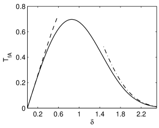
Figure 1:

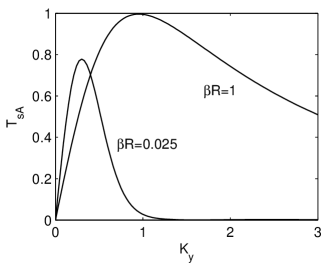
Figure 2:

References

- Bavassano et. al (2004) Bavassano, B., Pietropaolo, E., & Bruno, R., 2004, Ann. Geophys., 22, 689
- Barnes (1979) Barnes, A. 1979, Solar System Plasma Physics, C. Kennel, L. Lanzerotti and E. Parker, Amsterdam:North Holland, 249.
- Bhattacharjee & Ng (2001) Bhattacharjee, A., & Ng, C. S. 2001, ApJ, 548, 318
- Bigazzi et. al (2006) Bigazzi, A., Biferale, L., Gama, S. M. A., & Velli, M. 2006, ApJ, 638, 499
- Biskamp (2003) Biskamp, D. 2003, Magnetohydrodynamic Turbulence, Cambridge University Press, 232.
- Bodo et al. (2001) Bodo, G., Poedts, S., Rogava, A., & Rossi, P. 2001, A&A, 374, 337
- Breizman, Zakharov & Musher (1973) Breizman, B. N., Zakharov, V. E., & Musher, S. L. 1973, Sov. Phys. JETP, 64, 1297
- Bruno & Bavassano (1991) Bruno, R., & Bavassano, B. 1991, J. Geophys. Res., 96, 7841
- Chagelishvili, Rogava & Tsiklauri (1996) Chagelishvili, G. D., Rogava, A. D., & Tsiklauri, D. G. 1996, Phys. Rev. E, 53, 6028
- Chandran (2005) Chandran, B. D. G. 2005, Phys. Rev. Lett., 95, 265004
- Cho & Vishniac (2000) Cho, J., & Vishniac, E. 2000, ApJ, 539, 273
- Cranmer (2002) Cranmer, S. R. 2002, Space Sci. Rev., 101, 229
- Cranmer (2004) Cranmer, S. R. 2004, SOHO 15 Workshop - Coronal Heating, R.W. Walsh, J. Ireland, D. Danesy, & B. Fleck, Paris: European Space Agency (ESA SP-575), 109
- Cranmer & van Ballegooijen (2003) Cranmer, S. R., & van Ballegooijen, A. A. 2003, ApJ, 594, 573
- Cranmer & van Ballegooijen (2005) Cranmer, S. R., & van Ballegooijen, A. A. 2005, ApJS, 156, 265
- Fedoriuk (1983) Fedoriuk, M. V. 1983, Asymptotic methods for ordinary differential equations, Moscow:Nauka, 324
- Gogoberidze et al. (2004) Gogoberidze, G., Chagelishvili, G. D., Sagdeev, R. Z., & Lominadze, J. G. 2004, Phys. Plasmas, 11, 4672
- Gogoberidze (2006) Gogoberidze, G. 2006, astro-ph/0611894
- Goldreich & Lynden-Bell (1965) Goldreich P., & Lynden-Bell D. 1965, MNRAS, 130, 125
- Golderich & Sridhar (1995) Golderich, P., & Sridhar, S. 1995, ApJ, 438, 763
- Goldstein, Roberts & Matthaeus (1995) Goldstein, M. L., Roberts, D. A., & Matthaeus, W. 1995, ARA&A, 33, 283.
- Goldstein & Roberts (1999) Goldstein, M. L., & Roberts, D. A. 1999, Phys. Plasmas, 6, 4154
- Kopaleishvili (1995) Kopaleishvili, T. 1995, Collision theory: a short course, World Scientific Publishing Corporation, 38
- Lacombe & Mangeney (1980) Lacombe, C., & Mangeney, A. 1980, A&A, 277, 88
- Landau (1932) Landau, L. D. 1932, Phys. Z. Sowjetunion, 2, 46
- Landau & Lifschitz (1977) Landau, L. D., & Lifschitz, E. M. 1977, Quantum Mechanics (Non-Relativistic Theory), Oxford:Pergamon Press, 304
- Mahajan & Rogava (1999) Mahajan, S. M., & Rogava, A. D. 1999, ApJ, 518, 814
- Marsch & Tu (1990) Marsch, E., & Tu, C.-Y. 1990, J. Geophys. Res., 95, 945
- Montgomery et. al (1987) Montgomery, D., Brown, M. R., & Matthaeus, W. H. 1987, J. Geophys. Res., 92, 282
- McComas et al. (1998) McComas, D. J., Riley, P., Gosling, J. T., Balogh, A., & Forsyth, R. 1998, J. Geophys. Res., 103, 1955
- McComas et al. (2001) McComas, D. J., Goldstein, R., Gosling, J. T., & Skoug, R. M. 2001, Space Sci. Rev., 97, 99
- McComas et al. (2003) McComas, D. J., Elliott, H. A., Schwadron, N. A., Gosling, J. T., Skoug, R. M., & Goldstein, B. E. 2003, Geophys. Res. Lett., 30, 1517
- Müller et al. (2003) Müller, W.-C. , Biskamp, D., & Grappin, R. 2003, Phys. Rev. E, 67, 066302
- Oughton & Matthaeus (2005) Oughton, S., & Matthaeus, W. H. 2005, Nonlin. Proc. in Geophysics, 12, 299
- Poedts, Rogava & Mahajan (1998) Poedts, S., Rogava, A. D., & Mahajan, S. 1998, ApJ, 505, 369
- Poedts, Rogava & Mahajan (1999) Poedts, S., Rogava, A. D., & Mahajan, S. 1999, Space Sci. Rev., 87, 295
- Roberts et al. (1992) Roberts, D. A., Goldstein, M. L., Matthaeus, W. H., & Ghosh S. 1992, J. Geophys. Res. 97, 17115
- Rogava (2004) Rogava, A. D. 2004, Ap&SS, 293, 189
- Rogava & Gogoberidze (2005) Rogava, A. D., & Gogoberidze, G. 2005, Phys. Plasmas, 12, 052303
- Rogava, Poedts & Mahajan (2000) Rogava, A. D., Poedts, S., & Mahajan, S. M. 2000, A&A, 354, 749
- Schwadron et al. (2005) Schwadron, N. A., McComas, D. J., Elliott, H. A., Gloeckler, G., Geiss, J. & von Steiger, R. 2005, J. Geophys. Res., 110, A04104
- Shebalin et al. (1983) Shebalin, J. V., Matthaeus, W. H., & Montgomery, D. 2000, J. Plasma Phys., 29, 525
- Shergelashvili, Rogava, & Poedts (2005) Shergelashvili, B. M., Rogava, A. D., & Poedts, S. 2004, SOHO 15 Workshop - Coronal Heating, R.W. Walsh, J. Ireland, D. Danesy, & B. Fleck, Paris: European Space Agency (ESA SP-575), 437
- Shergelashvili, Poedts & Pataraya (2006) Shergelashvili, B. M., Poedts, S., & Pataraya, A. 2006, ApJ, 642, L73
- Stuekelberg (1932) Stuekelberg, E. C. J. 1932, Helv. Phys. Acta., 5, 369
- Swanson (1998) Swanson, D. G. 1998, Theory of Mode Conversion and Tunneling in Inhomogeneous Plasmas, New York:John Wiley and Sons
- Zener (1932) Zener, C. 1932, Proc. R. Soc. London Ser. A, 137, 696