The missing metals problem. III How many metals are expelled from galaxies?

Abstract

We revisit the metal budget at $z\simeq 2$, and include the contribution of the intergalactic medium. Past estimates of the metal budget indicated that, at redshift $z\simeq 2.5$, 90% of the expected metals were missing. In the first two papers of this series, we already showed that $\sim$30% of the metals are observed in all $z\sim 2.5$ galaxies detected in current surveys. This fraction could increase to $\la$ 60% if one extrapolates the faint end of the LF, leaving $>$40% of the metals missing. Here, we extend our analysis to the metals outside galaxies, i.e. in intergalactic medium (IGM), using (1) observational data and (2) analytical calculations. Our results for the two are strikingly similar: (1) Observationally, we find that, besides the small (5%) contribution of DLAs, the forest and sub-DLAs contribute subtantially to make $\la$30–45% of the metal budget, but neither of these appear to be sufficient to close the metal budget. The forest accounts for 15–30% depending on the UV background, and sub-DLAs for $\ga$2% to $\la$17% depending on the ionization fraction. Combining the metals in galaxies and in the IGM, it appears now that $>$65% of the metals have been accounted for, and the ‘missing metals’ problem is substantially eased. (2) We perform analytical calculations based on the effective yield–mass ($y_{\rm eff}$–$V_{c}$) relation, whose deficit for small galaxies is considered as evidence for supernova driven outflows. As a test of the method, we show that, at $z=0$, the calculation self-consistently predicts the total amount of metals expelled from galaxies. At $z=2$, we find that the method predicts that $25$–$50$% of the metals have been ejected from galaxies into the IGM, consistent with the observations ($\la$35%). The metal ejection is predominantly by $L_{B}<\frac{1}{3}L_{B}^{*}(z=2)$ galaxies, which are responsible for 90%  the metal enrichment, while the 50 percentile is at $L\sim\frac{1}{10}L^{*}_{B}(z=2)$. As a consequence, if indeed $50$% of the metals have been ejected from galaxies, 3–5 bursts of star formation are required per galaxy prior to $z=2$. The ratio between the mass of metals outside galaxies to those in stars has changed from $z=2$ to $z=0$: it was 2:1 or 1:1 and is now 1:8 or 1:9. This evolution implies that a significant fraction of the IGM metals will cool and fall back into galaxies.

1 Introduction

Locally, our picture of the metal (and baryon) budget has become more and more complete over the past few years (Fukugita et al., 1998; Fukugita & Peebles, 2004). Roughly speaking, 30% of the baryons are in the Ly$\alpha$ forest (Stocke et al., 2004), 50% are in a warm-hot phase (WHIM, Tripp et al., 2004), 5-10% are in the intra-cluster medium (ICM), and 10% are in stars. So, even-though WHIM (e.g. Sembach et al., 2004; Nicastro et al., 2005) and intra-group medium (Fukugita & Peebles, 2004) dominate the baryon budget, they contain a minor fraction ($<10$ %) of the metals. Indeed, about 80–90% of all the metals produced by type II and type Ia supernovae are locked in stars (10%) and stellar remnants (80%) such as white dwarfs, neutron stars and black holes (Fukugita & Peebles, 2004).

Ten Gyrs ago ($z\simeq 2.5$), the situation was very different. Most (90%) of the baryons were in the Ly$\alpha$ forest (e.g. Rauch et al., 1997; Penton et al., 2000; Schaye, 2001a; Simcoe et al., 2004), but our knowledge of metal abundances is still highly incomplete. In the past, it was realized that only a small fraction (20%) of the expected metals is accounted for when one adds the contribution of the Ly$\alpha$ forest ($N_{\hbox{{\rm H}{\sc\,i}}}=10^{13-17}$ cm^-2), damped Ly$\alpha$  absorbers (DLAs) ($N_{\hbox{{\rm H}{\sc\,i}}}>10^{20.3}$ cm^-2), and galaxies such as Lyman break galaxies (LBGs) (Pettini et al., 1999; Pagel, 2002; Pettini, 2003).

As discussed in Pettini et al. (2003), either the missing metals were expelled into the intergalactic medium (IGM) via galactic winds (as already discussed by Larson & Dinerstein, 1975) since LBGs drive winds (Adelberger et al., 2003; Shapley et al., 2003) much like the one seen locally (Lehnert & Heckman, 1996a; Dahlem et al., 1997; Lehnert et al., 1999; Heckman et al., 2000; Martin, 1999), or they are in a galaxy population not accounted for so far.

In Bouché et al. (2005) (hereafter paper I), we showed that only 5% (and $\la 9$%) of the expected metals are in submm selected galaxies (SMGs) and in Bouché et al. (2006) (hereafter paper II), we revisited the missing metal problem in light of the several new $z\sim 2$ galaxy populations, such as the ‘distant red galaxies’ (DRGs) and the ’BX’ galaxies. Paper II showed that the contribution of $z=2$ galaxies amounts to 18% for the star forming galaxies (including 8% for the rarer $K$-bright galaxies with $K_{s}<20$) and to 5% for the DRGs ($J-K>2.3$). Thus, adding the contribution of star-forming ‘BX’ galaxies, DRGs, and the SMGs, the total contribution of $z\sim 2$ galaxies is at least $18+5+5\sim 30$% of the metal budget. As shown in paper II, if one extrapolate these results to the faint end of the luminosity function, $\la$60% of the metals are in $z\sim 2$ galaxies, leaving $\ga 40$% missing.

The goal of this paper is to use observational data (section 2) and analytical calculations (section 3) to gain insights on the missing metals. In section 2, we include the contribution of metals in various gas phases, traced by QSO absorption lines. The dominant contributors are the forest (with $\log\hbox{$N_{\hbox{{\rm H}{\sc\,i}}}$}=10^{13\hbox{--}17}$) and the sub-DLAs with $\log\hbox{$N_{\hbox{{\rm H}{\sc\,i}}}$}=10^{19\hbox{--}20.3}$. We will show that neither the forest alone, nor sub-DLAs, can account for the remaining 40% of missing metals. In section 3, we explore the possibility that much of the remaining missing metals were ejected from galaxies based on ‘effective yield’ arguments. Namely, locally small galaxies have lost a significant fraction of their metals, reflected by their offset from the closed-box expected yield (e.g. Pilyugin & Ferrini, 1998; Köppen & Edmunds, 1999; Garnett, 2002; Dalcanton, 2006). Indeed, if all galaxies were evolving as ‘closed boxes’, their metallicity $Z$ would be inversely proportional to the gas fraction $\mu$, i.e. $Z\;\propto\;-\ln(\mu)$, and they would all reach approximately solar metallicity once they convert their gas into stars (e.g. Searle & Sargent, 1972; Audouze & Tinsley, 1976; Tinsley & Larson, 1978; Edmunds, 1990). The effective yield, $y_{\rm eff}$, which is simply the proportionality constant, is defined as:

$$y_{\rm eff} = \frac{Z}{\ln(1/\mu)}\;.$$ (1)

The ratio between the solar yield and $y_{\rm eff}$ gives the fraction of metals that were ejected (see section 3.1).

In the remainder of this paper, we used a $H_{0}=70~{}h_{70}$ ${\rm km\,s}^{-1}$ Mpc^-1, $\Omega_{M}=0.3$ and $\Omega_{\Lambda}=0.7$. We use a $Z_{\odot}=0.0189$ and a Salpeter IMF throughout.

2 The metal budget

2.1 The Metal Production Rate and Assumptions

Stellar nucleosynthesis and star formation govern the production of metals. Some of the metals remain locked up in stellar remnants or long-lived stars, some are returned into the interstellar medium (ISM) and another fraction is expelled into the intergalactic medium (IGM) via galactic winds and outflows. Under the assumption of instantaneous recycling approximation  (Searle & Sargent, 1972), the global metal production rate $\dot{\rho}_{Z}$ can be directly related to the star formation rate density (SFRD) $\dot{\rho}_{\star}$ through the IMF-weighted yield $<p_{z}>$ (Searle & Sargent, 1972; Songaila et al., 1990; Madau et al., 1996):

$$\dot{\rho}_{Z} = <p_{z}>\;\dot{\rho}_{\star}\;,\hbox{with}$$ (2)

$$<p_{z}> = \int\mathrm{d}m\;p_{z}(m)m\phi(m)\;,$$ (3)

where $\phi(m)$ is the IMF, and $p_{z}(m)$ is the metal yield for stars of mass $m$. The total expected amount of metals $\rho_{Z,\rm expected}$ formed by a given time $t$ is the integral of Eq. 2 over time.

The IMF-weighted yield in Eq. 2 is equal to $\frac{1}{42}$ or 2.4% (Madau et al., 1996) using a Salpeter IMF and the type II stellar yields (for solar metallicity) $p_{z}(m)$ from Woosley & Weaver (1995) . It should be noted that changing the IMF (or the low mass end) will change both $\dot{\rho}_{\star}$ and $p_{z}$ in the same way leaving $\rho_{Z}$ unchanged since $\dot{\rho}_{\star}$ is measured from a stellar luminosity density $\rho_{L}$. In other words, the metal production rate is directly related to the mean luminosity density $\rho_{L}$ via $\rho_{L}=\epsilon\;\dot{\rho}_{Z}$, where $\epsilon$ is independent of the IMF (Songaila et al., 1990; Madau et al., 1996).

The SFRD in Eq. 2, $\dot{\rho}_{\star}$, is inferred from rest-frame UV surveys and at redshifts greater than 1, appears to be constant from a redshift of $z\sim 4$ to $z\sim 1$ at a level of about $\dot{\rho}_{\star}\simeq 0.1\;h_{70}$ M_⊙ yr^-1 Mpc^-3 once corrected for dust extinction (Lilly et al., 1996; Madau et al., 1996; Steidel et al., 1999; Dickinson et al., 2003; Giavalisco et al., 2004; Drory et al., 2005; Hopkins, 2004; Hopkins & Beacom, 2006; Panter et al., 2006; Fardal et al., 2006).

In order to compute $\rho_{Z}(t)$ from Eq. 2, we parameterize the SFRD, $\dot{\rho}_{\star}$, as shown in Fig. 1 (bottom). The solid line shows $\dot{\rho}_{\star}(t)$ parameterized by Cole et al. (2001) for an extinction of $E(B-V)=0.10$. The dashed line shows $\dot{\rho}_{\star}(t)$ set to $0.1\;h_{70}$ M_⊙ yr^-1 Mpc^-3 above redshift $z=1$, and linearly proportional to $z$ below $z=1$. The dotted line shows $\dot{\rho}_{\star}(t)$ set $0.15\;h_{70}$ M_⊙ yr^-1 Mpc^-3 at high redshifts, while keeping the same decline below $z\simeq 1$.

We first check that the integrated SFRD gives the amount of stars using $\rho_{\star}=(1-R)\cdot\int_{0}^{t}\mathrm{d}t\;\dot{\rho}_{\star}(t)\;,$ $R$ is the mass fraction recycled into the ISM. For a Salpeter IMF, $R$ equals $0.28$ (Cole et al., 2001). The top panel shows ${\rho}_{\star}(t)$ for the three parameterizations. Both the solid and dashed curves reach the local stellar mass density shown by the shaded area for (Cole et al., 2001) and the filled symbol for Bell et al. (2003) . The agreement was also found by others (e.g. Rudnick et al.,, 2003; Dickinson et al., 2003; Rudnick et al.,, 2006). Recent studies pointed to some tension between the local $\rho_{\star}(z=0)$ and the integrated SFRD (Hopkins & Beacom, 2006; Fardal et al., 2006).

The overlap between different galaxy populations is very much unknown. With respect to the SFRD, two populations, LBGs and SMGs, reaches similar levels (e.g. Steidel et al., 1999; Chapman et al., 2005), after a dust-correction for LBGs of a factor of $\sim 5$. Should the SFR of these two populations be added, which would double the SFRD at $z=2$? The dotted line in Fig. 1 shows that, if one doubles the SFRD at $z=2$, one over-predicts the observed stellar density $\rho_{\star}(z=0)$ by $\sim~{}40$% if the SFRD is increased by 50%. Thus, there is little room to add the SMG contribution to the SFRD at high-redshifts ($\sim 0.1~{}\hbox{M${}_{\odot}$\,yr${}^{-1}$\, Mpc${}^{-3}$}$), given the large dust-correction applied to LBGs that already encompasses various galaxy populations. This conclusion is very general and does not depend on the tension between $\rho_{\star}(z=0)$ and the integral of the SFRD discussed in Hopkins & Beacom (2006); Fardal et al. (2006), adding the SMGs, i.e. doubling the SFR at $z\sim 2$, would increase the discrepancy further.

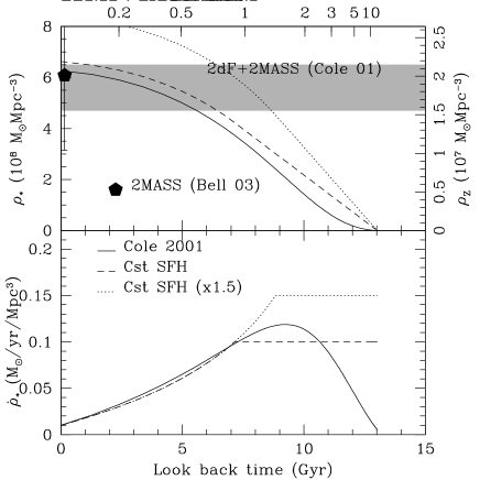
Figure 1: Bottom panel: Star formation history (SFH) of the universe. The solid line shows $\dot{\rho}_{\star}(t)$ parameterized by Cole et al. (2001) for a extinction of $E(B-V)=0.10$. The dashed line shows $\dot{\rho}_{\star}(t)$ set to $0.1\;h_{70}$ M_⊙ yr^-1 Mpc^-3 beyond redshift $z=1$, and linearly proportional to $z$ below $z=1$. The dotted line shows $\dot{\rho}_{\star}(t)$ set $0.15\;h_{70}$ M_⊙ yr^-1 Mpc^-3 at high redshifts, while keeping the same behavior at low redshifts. Top panel: Mass stellar build-up (${\rho}_{\star}(t)$) for the same three parameterizations. The left axis shows the visible stellar density ($(1-R)\cdot\int$ SFH), where $R$ is the recycled fraction, while the right axis shows the metal production ($<p_{z}>\cdot\int$ SFH). Both the solid and dashed curves reach the observational constraint of $\rho_{\star}(z=0)$ (Cole et al., 2001), shown by the shaded area. The dotted line clearly overshoots the observations, leaving little room on the SFR at high-redshifts. As a consequence, the contributions of LBGs (dust-corrected, Steidel et al., 1999) and SMGs (Chapman et al., 2005) cannot simply be added.

2.2 The expected amount of metals

The right axis of Fig.1(top) shows the metal density $\rho_{Z}(t)$ found from integrating Eq. 2 over time. From this figure, one sees that at $z=0$, the amount of metals formed (by type II supernovae) is expected to be 

$$\rho_{Z,\rm exp.}(z=0) = 2.13\times 10^{7}\;\frac{<p_{z}>}{1/42}~{}\hbox{M${}_{\odot}$\, Mpc${}^{-3}$}\;,$$ (4)

if we integrate the SFH from $t=13.7$ Gyr until the present. As a cross-check, this number (Eq. 4) is consistent with the findings of Fukugita & Peebles (2004). Indeed, their Table 3 list the amount of metals in different classes of objects. Given that the mean yield $<p_{z}>=1/42$, used in Eq. 4, is calculated including only stars with $m>10$ M_⊙, we exclude the contribution from main sequence (MS) stars and from white dwarfs from the table of Fukugita & Peebles (2004), and find that the $z=0$ metal density is $\rho_{Z,\rm observed}(z=0)\sim 2.3\times 10^{7}$ M_⊙  Mpc^-3, which is quite close to Eq. 4. In the remainder of this paper, we will refer to these numbers as ‘the $z=0$ metal density’, but one should keep in mind that it does not include the contribution from white dwarfs (SN Ia) and locked in the MS (see Table 6) since we will focus on the type II yields at $z\simeq 2.5$ throughout this paper.

At high-redshifts, if we integrate the SFH, from $z=4$ to $z=2$, corresponding to a time interval of 1.68$\;h_{70}^{-1}$ Gyrs, the expected amount of metals formed is

$$\rho_{Z,\rm exp.}(z=2) \simeq 4.0\times 10^{6}\frac{\dot{\rho}_{\star}}{0.1}\frac{<p_{z}>}{1/42}\;h_{70}^{0}~{}\hbox{M${}_{\odot}$\, Mpc${}^{-3}$}\;\hbox{or}$$ (5)

$$\overline{Z}_{b} \simeq 0.035\frac{<p_{z}>}{1/42}\frac{0.0189}{Z_{\odot}}\;h_{70}^{-1}\;\;\hbox{}$$

By comparing Eq. 5 with Eq. 4, and from Fig. 1, one sees that about 1/4 or 1/5 of the metals are already produced by $z=2$ (e.g. Pagel, 2002; Pettini, 2003, 2006). This is consistent with the stellar mass density evolution studies (e.g. Rudnick et al.,, 2003, 2006; Panter et al., 2006) that have found similar amount of evolution.

If we integrate the constant SFH (at 0.1 M_⊙ yr^-1 Mpc^-3) from $z=10$ to $z=2$, then the amount of metals formed by $z=2$ is

$$\rho_{Z,\rm exp.}(z>2) \simeq 6.4\times 10^{6}\frac{<p_{z}>}{1/42}\hbox{$h_{70}^{0}$~{}\hbox{M${}_{\odot}$}~{}Mpc${}^{-3}$}\;.$$ (6)

Table 1: The metal budget for $z\sim 2$ galaxies.

Class	$\rho_{Z}$	$\Omega_{Z}$	$\overline{Z}_{b}$	$\rho_{Z}/\rho_{Z,\rm tot}$	Ref	Note
	(M⊙  Mpc-3)		($Z_{\odot}$)	(%)
SMGs	$<3.6\times 10^{5}$	$<2.7\times 10^{-6}$	$<$0.0031	$<$9	1	$>3$mJy ($Z=2\;Z_{\odot}$)
SMGs	$1.8\times 10^{5}$	$1.6\times 10^{-6}$	0.0015	5	1	$>3$mJy ($Z=1\;Z_{\odot}$)
BX	$3.8\times 10^{5}$	$2.8\times 10^{-6}$	0.0033	10	2	$>L^{*}$
BX$+K<$20	$3.0\times 10^{5}$	$2.2\times 10^{-6}$	0.0027	8	2	$>L^{*}$
DRGs	$2.0\times 10^{5}$	$1.5\times 10^{-6}$	0.0018	5	2	$J-K>2.3$
Total Observed	$1.1\times 10^{6}$	$7.8\times 10^{-6}$	0.010	$\sim$30	2	$>L^{*}$
Total Inferred	$2.2\times 10^{6}$	$1.6\times 10^{-5}$	0.020	$\sim$60	2	all $L$
Missing				$>40$		all $L$

2.3 Metals in galaxies

Some argued that the dusty ISM of submm galaxies could harbor most of the remaining missing metals. However, in paper I, we showed that the remaining missing metals cannot be in SMGs based on direct metallicity and gas mass measurements. Only 5% (and $\la 9$%) of the expected metals are in SMGs.

The second paper of this series (Paper II) showed that the contribution of $z=2$ galaxies amounts to 10% for the star forming ‘BX’ galaxies, to 8% for the rarer $K$-bright ‘BX’ galaxies with $K_{s}<20$, and to an additional 5% for the DRGs ($J-K>2.3$).

We note that the numbers quoted in paper II for the BX galaxies were technically based on their stellar mass estimates (using a Salpeter IMF) combined with their metallicity, i.e. without the contribution of the ISM which was unconstrained at the time. However, based on H$\alpha$ flux measurement, Erb et al. (2006) estimated the gas fractions of ‘BX’ galaxies to be $\sim 50$%. Thus, the contribution of the ‘BX’ galaxies alone may be as high as 15%. DRGs are generally likely to be poorer in gas. But, given that stellar masses $M_{\star}$ of high-redshift galaxies are known to be overestimated (for a Salpeter IMF) when one compares $M_{\star}$ to their dynamical masses $M_{\rm dyn}$ (see Forster Schreiber et al.,, 2006), our estimates in paper II can be viewed as inclusive of all the baryons (gas and stars).

All in all, the total contribution of the known $z\sim 2$ populations is $\sim 30$% (see also Pettini, 2006) of the metal budget corresponding to a cosmic metal density of

$$\rho_{Z,\rm galaxies}\simeq 1.1\times 10^{6}\;\hbox{M${}_{\odot}$\, Mpc${}^{-3}$}\;.$$ (7)

Furthermore, since most high-redshift surveys detect galaxies to a luminosity comparable to $L^{*}$, in paper II, we estimated the contribution of the fainter galaxy population using a metallicity-luminosity relation. We found that the $<L^{*}$ galaxy population could double this sum. In other words, currently known galaxy populations at $z=2$ can only account for 30 to 60% of the metals expected, and $\ga 40$% are unaccounted for (see summary in Table 1).

2.4 Metals in absorption lines

We separate our analysis of the metals in the IGM according to the H i column density. The forest with $\hbox{$N_{\hbox{{\rm H}{\sc\,i}}}$}<10^{17}$ cm^-2  is discussed in section 2.4.1, sub-DLAs with $10^{19}<\hbox{$N_{\hbox{{\rm H}{\sc\,i}}}$}<10^{20.3}$ cm^-2  in section 2.4.2, and DLAs with $\hbox{$N_{\hbox{{\rm H}{\sc\,i}}}$}>10^{20.3}$ cm^-2 in section 2.5.

2.4.1 Metals in the forest

Table 2: Metals in the forest.

Element	$\rho_{X}$	$\Omega_{X}$	$\rho_{Z}$	$\Omega_{Z}$	$\overline{Z}_{b}$	$f$	Method	Ref	UVB
	(M⊙  Mpc-3)		(M⊙  Mpc-3)			(%)
C	$3.1\times 10^{4}$	$2.3\times 10^{-7}$	$3\times 10^{5}$	$2.2\times 10^{-6}$	0.0026	8	C iv HPOD	(1)	soft
C	$4.9\times 10^{4}$	$3.6\times 10^{-7}$	$4.7\times 10^{5}$	$3.4\times 10^{-6}$	0.0041	13	C iv HPOD	(2)	hard
Si	$4.6\times 10^{4}$	$3.4\times 10^{-7}$	$1.2\times 10^{6}$	$8.6\times 10^{-6}$	0.0100	30	Si iv CPOD	(3)	soft
O	$2.4\times 10^{5}$	$2.0\times 10^{-6}$	$4.6\times 10^{5}$	$3.4\times 10^{-6}$	0.0040	12	O vi	(2)	hard
O	$7.0\times 10^{5}$	$5.0\times 10^{-6}$	$1.2\times 10^{6}$	$8.4\times 10^{-6}$	0.010	30	O vi	(2)	soft
O	$1.7\times 10^{5}$	$2.3\times 10^{-6}$	$5.2\times 10^{5}$	$3.9\times 10^{-6}$	0.0046	13	O vi	(4)	hard
Summary	$3.5\times 10^{5}$	$2.5\times 10^{-6}$	$5.8\times 10^{5}$	$4.2\times 10^{-6}$	$<$0.0050	$<$15–30

In the low-density IGM (with $\hbox{$N_{\hbox{{\rm H}{\sc\,i}}}$}<10^{17}$ cm^-2), C, Si, and O, as traced by C iv, Si ivand O vi, are useful probes of the metals contained in the IGM (e.g. Songaila, 2001; Aguirre et al., 2002; Schaye et al., 2003; Pettini et al., 2003; Simcoe et al., 2004; Aguirre et al., 2004; Songaila, 2005).

Several approaches have used to estimate the metal content of the IGM using these ions. For instance, the ratio of C iv to H i using the pixel optical depth method (e.g. Aguirre et al., 2002) can be converted into carbon abundances given an ionization correction (e.g. Schaye et al., 2003). These can be computed as a function of density $n_{\hbox{{\rm H}{\sc\,i}}}$ for a given UV background (UVB) model using codes such as CLOUDY. Hydrodynamical simulations can provide interpolation tables of the density (and temperature) as a function of the Ly$\alpha$ optical depth (and redshift). This was done by Schaye et al. (2003), under several assumptions regarding the UVB model used in generating the ionization corrections. For a UVB from Haardt & Madau (2001) including quasars and galaxies (hereafter ‘soft UVB’), they found

$$\Omega_{C,\rm IGM} \simeq 2.3\times 10^{-7}\;10^{\hbox{[C/H]}+2.8}\;\left(\frac{\Omega_{b}}{0.045}\right)$$

$$\rho_{C,\rm IGM} \simeq 3.1\times 10^{4}\;10^{\hbox{[C/H]}+2.8}$$ (8)

This corresponds to a metallicity contribution of $\rho_{Z,\rm IGM}\simeq 3\times 10^{5}\;\hbox{M${}_{\odot}$\, Mpc${}^{-3}$}$, or only about 8% of the metal budget This study had a threshold at $\tau_{\hbox{{\rm H}{\sc\,i}}}\sim 1$, corresponding to $\hbox{$N_{\hbox{{\rm H}{\sc\,i}}}$}\;\sim\;10^{13.5}$ cm^-2. The work of Simcoe et al. (2004), based on line fitting and on different assumptions, gave similar results ([C/H]=$-2.2$) and would be almost identical ([C/H]=$-3.1$) under similar assumptions about the UVB. This study had a threshold at $\hbox{$N_{\hbox{{\rm H}{\sc\,i}}}$}>10^{14}$ cm^-2.

As for silicon abundances, the firmest estimates are provided by Aguirre et al. (2004), who studied the forest metallicity by analyzing Si iv and C iv pixel optical depth derived from high quality Keck and VLT spectra. They find that [Si/C] ranges from [Si/C] $\simeq 0.25$ (for a very soft UVB) to [Si/C] $\simeq 1.5$ (for the ‘hard’ UVB). For a fiducial ‘soft’ UVB model, they fit a value of [Si/C]$=0.77\pm 0.05$ for gas in over-densities of $\delta>3$ or $N_{\hbox{{\rm H}{\sc\,i}}}>10^{14}$ cm^-2. This then gives a metallicity contribution of [Si/H]$=-2.03\pm 0.14$, corresponding to

$$\Omega_{Si,\rm IGM} \simeq 3.4\times 10^{-7}\;10^{\hbox{[Si/H]}+2.0}\;\left(\frac{\Omega_{b}}{0.045}\right).$$

$$\rho_{Si,\rm IGM} \simeq 4.6\times 10^{4}\;10^{\hbox{[Si/H]}+2.0}\;\hbox{M${}_{\odot}$\, Mpc${}^{-3}$}\;.$$ (9)

Since about 3–5% of type II supernova metal production is Si (Samland, 1998), this corresponds to

$$\rho_{Z,\rm IGM} \simeq 1.16\times 10^{6}\frac{y_{\rm Si}}{0.04}\;\hbox{M${}_{\odot}$\, Mpc${}^{-3}$},$$ (10)

$$\overline{Z}_{b} \simeq 0.010,$$

i.e. $\sim$30% of the metal budget.

This result is highly sensitive to the hardness of the assumed UVB, since softening the UVB (for example) lowers both the inferred [C/H] and the inferred [Si/C]. However, the UVB hardness has the opposite effect on [O/C] and [O/H], so they are also quite useful to examine.

Using a ‘hard’ UVB, Simcoe et al. (2004) measured [C,O/H] from which they infer $\Omega_{\rm O}\simeq 1.4\times 10^{-6}\;h^{-1}\;\simeq 2.0\times 10^{-6}\;h_{70}^{-1}$ using [O/C]$\simeq 0$ set by the UVB. The corresponding density of Oxygen is $\rho_{\rm O}\simeq 3.4\times 10^{5}~{}\hbox{M${}_{\odot}$\, Mpc${}^{-3}$}$, or

$$\rho_{Z,\rm forest} \simeq 4.6\times 10^{5}\frac{y_{\rm O}}{0.60}\;\hbox{M${}_{\odot}$\, Mpc${}^{-3}$},,$$ (11)

$$\overline{Z}_{b} \simeq 0.004,$$

about 12% of the metal budget. Using a ‘soft’ UVB gives [O/C] $\simeq 0.5$ which is more in line with the relative abundances seen in other metal-poor environments such as halo stars (Cayrel et al., 2004), and increases the median [O/H] by $\sim 0.15$ dex, but a calculation of $\Omega_{\rm O}$ under this assumption was not provided. If the [C/H] values of Schaye et al. (2003) are used with [O/C]=0.5 (which is consistent with results using the pixel optical depth technique; see Dow-Hygelund et al., in prep.), we would obtain $\bar{Z}_{b}\simeq 0.01$, or $\sim 30\%$ of the metal budget.

Instead of looking at [O/H], Bergeron & Herbert-Fort (2005) searched for O vi where the identification of the systems is done with C iv, i.e. independently of $N_{\hbox{{\rm H}{\sc\,i}}}$. These studies found two populations of O vi absorbers. The first population is metal poor (with [O/H]$\simeq-2.0$) and has narrow line width ($b\la 12$ ${\rm km\,s}^{-1}$), indicative of photoionization. The second (and new) population is much more metal rich with [O/H]$\simeq-0.33$, and has larger line widths. Globally, they found that $\Omega_{\hbox{{\rm O}{\sc\,vi}}}=3.5\times 10^{-7}$, of which the metal-rich population contributes 35%. Using a ionization correction $\hbox{{\rm O}{\sc\,vi}}/$O=0.15 (assuming a hard UVB), Bergeron & Herbert-Fort (2005) infer a Oxygen density $\Omega_{\rm O}=2.3\times 10^{-6}$, which corresponds to:

$$\rho_{Z,\rm forest} \simeq 5.2\times 10^{5}\frac{y_{\rm O}}{0.60}\;\hbox{M${}_{\odot}$\, Mpc${}^{-3}$},$$ (12)

$$\overline{Z}_{b} \simeq 0.0046,$$

or 13 % of the metal budget, similar to the estimate of Pettini (2006).

The results from the literature are summarized in Table 2. The Ly$\alpha$ forest mean metallicity (by mass) is $\overline{Z}_{b}\simeq 0.005$–0.010 (depending on the UVB model assumed and tracer element used) and indicates that it holds $\sim 15-30\%$ of the $z=2$ metal budget (see also Pettini, 2006). Using carbon as a tracer leads to a somewhat smaller estimate .

Assuming that the intergalactic metal budget is dominated by warm ($\sim 10^{4}\,$K) photoionized gas, the contribution of the forest is 15 (30)%  depending on the UVB. If the UVB were a bit harder (or softer), it would decrease (increase) slightly 1 or 2 elements, but the other element(s) would increase (decrease). In particular, in order to have a UVB that yields a [Si/O] ratio consistent with type II SNe, there is little room to change the 15-30% contribution.

However, it is important to note that if a significant reservoir of metals is hidden in hot ($\ga 10^{5}\,$K) collisionally ionized gas, these would evade detection in C iv and Si iv, so that the ionization corrections employed in the calculations cited above would underestimate the true metal content. For example, in simulations including feeback by Oppenheimer & Davé (2006), heating of the gas hides a significant fraction of the carbon mass, so that the ionization fraction of carbon is than in Schaye et al. (2003) by a factor of almost three. This might bring the carbon metallicity more in line with silicon and oxygen; which might be affected by prevalent hot gas to a lesser (though currently unquantified) degree.

2.4.2 Lyman Limit Systems (LLS)

Lyman limit systems (LLS) with $\hbox{$N_{\hbox{{\rm H}{\sc\,i}}}$}>10^{17}$ cm^-2 are prime candidates for harboring the missing metals. Indeed, some of them are highly ionized (because they have a lower H i column density and might therefore not be sufficiently self-shielded), and if a small fraction of LLSs are metal rich (as already seen in Charlton et al., 2003; Ding et al., 2003; Masiero et al., 2005), they could contribute significantly to the metal budget (e.g. Péroux et al., 2006; Prochaska et al., 2006).

However, no model-independent constraints exist for LLS with $10^{17}<\hbox{$N_{\hbox{{\rm H}{\sc\,i}}}$}<10^{19}$ cm^-2, but progress is being made for absorbers with $10^{19}<\hbox{$N_{\hbox{{\rm H}{\sc\,i}}}$}<10^{20.3}$ cm^-2, also called sub-DLAs, since damping wings are clearly visible at such HI column densities (e.g. Péroux et al., 2006).

Based on direct measures of the neutral gas mass and metallicity of a sample of sub-DLAs, Kulkarni et al. (2006) calculated the amount of metals of these systems to be $Z_{b}=6.4\times 10^{-4}$, or $\Omega_{Z}\simeq 5.1\times 10^{-7}$ using no ionization correction $f$, i.e. $f=1.0$ where $f=1/(1-x)$ for an ionization fraction $x$. This corresponds to:

$$\rho_{Z,\rm sub-DLAs}\ga 6.9\times 10^{4}\left(\frac{f}{1.0}\right)\frac{Z}{0.15Z_{\odot}}~{}\hbox{M${}_{\odot}$\, Mpc${}^{-3}$},$$ (13)

or about 2% of the metal budget. Eq. 13 is a lower limit since $x=0$ was assumed. However, Kulkarni et al. (2006) emphasize that $x$ is model dependent and that different sub-DLAs might have very different ionization fraction even at similar $N_{\hbox{{\rm H}{\sc\,i}}}$ (see Dessauges-Zavadsky et al. (2006) for a sample of 13 ionized fraction estimates).

Indeed, Prochaska et al. (2006) deduce $x$=0.9 for one of their sub-DLA for which they run photo-ionisation modelling and assume $x$=0.1 for the other one. Based on this single measure, they estimated the amount of metals in sub-DLAs (i.e. assuming $x$=0.9) to be $\Omega_{Z}\simeq 5\;10^{-6}$ or:

$$\rho_{Z,\rm sub-DLAs}\la 6.8\times 10^{5}\left(\frac{f}{10}\right)\frac{Z}{0.1Z_{\odot}}~{}\hbox{M${}_{\odot}$\, Mpc${}^{-3}$},$$ (14)

or 17% of the metal budget. This result used a mean metallicity for the entire population of $0.1\;Z_{\odot}$ from Péroux et al. (2003).

Given the potentially large reservoir of metals in sub-DLAs, progress in this field is advancing rapidly (Péroux & et al., 2006; Prochaska et al., 2006).

2.5 Damped Ly$\alpha$ absorbers (DLAs)

Table 3: Metals in the IGM.

Class	$\rho_{Z}$	$\Omega_{Z}$	$\overline{Z}_{b}$	$\rho_{Z}/\rho_{Z,\rm tot}$	Ref	Note
	(M⊙  Mpc-3)		($Z_{\odot}$)	(%)
DLA ($\hbox{$N_{\hbox{{\rm H}{\sc\,i}}}$}>10^{20.3}$)	$2.0\times 10^{5}$	$1.5\times 10^{-6}$	0.0018	5.0	1
sub-DLAs ($10^{19}<\hbox{$N_{\hbox{{\rm H}{\sc\,i}}}$}<10^{20.3}$)	$6.8\times 10^{5}$	$5.0\times 10^{-6}$	0.0060	$<$17	2	with $x=0.9$
sub-DLAs ($10^{19}<\hbox{$N_{\hbox{{\rm H}{\sc\,i}}}$}<10^{20.3}$)	$6.9\times 10^{4}$	$5.1\times 10^{-7}$	0.0006	$>$2	3	with $x=0.0$
LLS ($10^{17}<\hbox{$N_{\hbox{{\rm H}{\sc\,i}}}$}<10^{19}$)	…	…	…	…
Forest ($\hbox{$N_{\hbox{{\rm H}{\sc\,i}}}$}<10^{17}$)	$5.8\times 10^{5}$	$4.2\times 10^{-6}$	0.005	$<$15	4
IGM Metals: Total	$1.5\times 10^{4}$	$1.1\times 10^{-5}$	0.011	$<37$	excluding LLS

Because (i) $\Omega_{\hbox{{\rm H}{\sc\,i}}}$ appears to evolves by at most a factor of two to redshift zero (Rosenberg & Schneider, 2003; Zwaan et al., 2005), and that (ii) the metallicity evolution in DLAs (Prochaska & Wolfe, 2000; Kulkarni & Fall, 2002; Kulkarni et al., 2005; Prochaska et al., 2003) is much milder than the metallicity evolution seen in galaxies (Lilly et al., 2003), one is forced to conclude that DLAs ‘do not trace everything’, but are just tracing the gas in the same physical conditions at all redshifts.

Regardless of the origin of the gas, from an observational standpoint, DLAs are twenty times more metal rich than the forest (Pettini et al., 1999; Prochaska & Wolfe, 1997; Vladilo et al., 2000; Prochaska et al., 2003). But given than they account for 2–3% of the baryons (Péroux et al., 2003) with $\Omega_{\rm DLA}=1.5\times 10^{8}\;h_{70}^{1}\hbox{M${}_{\odot}$\, Mpc${}^{-3}$}$, only 5% the metals, i.e.

$$\rho_{Z,\rm DLA}=2\times 10^{5}\hbox{M${}_{\odot}$\, Mpc${}^{-3}$}\;,$$ (15)

are in DLAs given their mean metallicity of $-1.15$ or 0.07$Z_{\odot}$ (e.g. Pettini et al., 1999; Kulkarni et al., 2005). 

There seem to be little amount of dust in DLAs as measured directly from depletion pattern (e.g. Dessauges-Zavadsky et al., 2002) or from the attenuation of the QSO light (e.g. Murphy & Liske, 2004; York et al., 2006; Wild et al., 2006). The latter method indicates that $E(B-B)<0.01$ in DLAs. However, they have been claims that dusty DLAs would be missed from optically selected quasar samples altogether as argued by Vladilo & Péroux (2005). These authors find that the missing fraction of DLAs is a strong function of the limiting magnitude of the quasar sample and they concluded that (i) we might be missing as much as 30-50% of $\Omega_{\hbox{{\rm H}{\sc\,i}}}$ for QSO surveys down to $r=20.5$, and (ii) averaged DLA metallicities could be 5 to 6 times higher than currently observed. Up to now, the magnitude range $r=19.5$ to $r=20.5$ has been largely unexplored, and it is where most of the bias due to dust could be more significant.

Recently, Herbert-Fort et al. (2006) identified from SDSS-DR3 a large sample of 435 metal strong QSO absorption line selected using EW(Zn), with properties similar to the metal strong DLA of Prochaska et al. (2003). From their sample, they infer a global fraction of metal strong DLAs of 5% down to $r=19.5$.

In order to estimate the additional contribution to $\rho_{Z}$ from metal-rich dusty DLAs, we examine the various possibilities. In the scenario of Vladilo & Péroux (2005), the averaged metallicity of DLAs should be 5 times higher than the observed mean DLA metallicity of $Z/Z_{\odot}\simeq 0.07$. Given their estimate of a ’dusty DLA’ fraction missed in current surveys of 30% (by mass), the metallicity of this populations might be close to be around solar (but not much higher). If we take their metallicity to be $Z\sim 0.5Z_{\odot}$, 7 times that of ‘traditional’ DLAs, the amount of metals in this population of dusty DLAs is estimated to be:

$$\rho_{Z,\rm DLA+} = 30\%\cdot\Omega_{\rm DLA}\cdot 0.5Z_{\odot}$$ (16)

$$\simeq 4.7\times 10^{5}\;\frac{f_{DLA\rm rich}}{0.30}\frac{Z_{DLA\rm rich}}{0.5}~{}\hbox{M${}_{\odot}$\, Mpc${}^{-3}$}\,,$$

or about 12% of the metal budget; a non-negligible contribution. If the fraction of metal rich systems is closer to $\sim$5% (Herbert-Fort et al., 2006) with a mean metallicity of $0.3\;Z_{\odot}$, then Eq. 16 is reduced by a factor of 10, and the contribution of dusty DLAs is not significant. This population of dusty DLAs could contribute significantly to the metal budget.

In Table 3, we summarize the metal budget for the IGM. The sum for DLAs, sub-DLAs and the forest reaches about $<35$ to $<$40%, which is barely what is required to close the metal budget.

2.6 QSOs and AGN feedback

The contribution of QSOs to the cosmic metal budget is usually not included due to their very low number density, $n_{\rm QSO}\la 10^{-6}$ Mpc^-3 (e.g. Croom et al., 2004). But, QSOs appear to have reached solar metallicity (e.g. Hamann et al., 2002, 2004) based on independent analyses of quasar broad emission lines and intrinsic narrow absorption lines (see also D’Odorico et al., 2004). Given that their life time is relatively short ($\tau\la 10$ Myr, i.e. duty cycle large $\ga 100$), their contributions can be much larger if they contain large amount of gas. From CO observations, it has been noted that QSOs contain less gas than SMGs by a factor of $\sim 4$ (Greve et al., 2005), so we expect their contribution to be less than that of the SMGs. Typically, QSOs have $\sim\;10^{10}$ M_⊙ of gas (e.g. Hainline et al., 2004). We find that, the comoving amount of metals in QSOs is then:

$$\rho_{Z,\rm QSO}=2\;\times\;10^{4}\frac{n_{\rm QSO}}{10^{-6}}\frac{f}{100}\frac{M_{\rm gas}}{10^{10}}\;\hbox{M${}_{\odot}$\, Mpc${}^{-3}$}\,$$ (17)

or less than 1% of the expected metals.

Thus, even if QSOs expel most of their gas, they cannot contribute to the metal budget at more than the percent level. In fact, Nesvadba et al. (2006) studied the kinematics of the outflow powered by the radio galaxy MRC1138$-$262, and estimated an outflow rate 300-400 M_⊙ yr^-1. From the outflow rate, they estimated the contribution to $\rho_{Z}$ from AGN feedback assuming that all QSOs undergo a powerfull radio phase similar to that of MRC1138$-$262 (using a duty cycle of 300). They found that they could contribute to 0.1—30$\times 10^{4}$ M_⊙  Mpc^-3 of metals, i.e. at most 10%, and the most likely value is $1\times 10^{4}$ M_⊙  Mpc^-3 or 0.3% given that QSOs outflows are not likely to expel more metals than their gas reservoir (Eq. 17) . We thus view that AGN feedback is unlikely to contribute significantly to the enrichment of the IGM, but will significantly affect the evolution of massive objects (e.g. Croton & et al.,, 2005; Nesvadba et al., 2006; Best et al., 2006)

3 How many metals are ejected from small galaxies?

In this section, we use simple analytical calculations based on the effective yield $y_{\rm eff}\equiv Z/\ln(1/\mu)$ (Eq. 1) to argue that, at $z=2.$, 25-50% of the metals are ‘outside’  galaxies. First, we test our method at $z=0$ in section 3.2, and then repeat it at $z=2.5$ in section 3.3.

3.1 The contribution of metals lost from galaxies

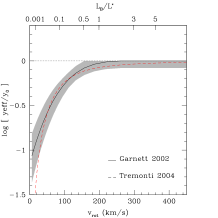
Figure 2: Effective yield ($y_{\rm eff}$) normalized to the value expected from a close box model $y_{0}$. The solid line shows the relation parameterized by Garnett (2002), and the dashed line shows the relation obtained by Tremonti et al. (2004) using SDSS data. The shaded area represent the allowed range from the observations.

At $z=0$, evidence for enriched material being ejected by galaxies comes from the mass (or luminosity)–metallicity relation (e.g. Garnett, 2002; Pilyugin et al., 2004; Tremonti et al., 2004). Essentially any chemical model would predict that a galaxy (as it turns its gas into star) reaches solar metallicity (e.g. Edmunds, 1990) even with infall of primordial gas. Once the energy of SN is larger than the gravitational energy of the gas, the remaining gas could be expelled, resulting in a mass–metallicity relation since the gravitational energy will depend on the mass (Larson, 1974).

Another signature of gas losses come from the effective yield (Eq. 1), which measures how far a galaxy is from a ‘closed-box’ evolution. A galaxy that has evolved as a closed-box would obey a simple linear relationship between gas metallicity and gas fraction, the slope being the effective yield, i.e. $Z\;=y_{\rm eff}\;\times\;\ln(1/\mu)$ (Eq. 1).

Fig. 2 shows the effective yield as a function of rotational velocity $V_{c}$. The solid line shows the relation parameterized by Garnett (2002), and the dashed line shows the relation obtained by Tremonti et al. (2004) using SDSS data. The shaded area represent the allowed range from the observations.

This effective yield has two important properties relevant for this paper. First, as it has been shown many times (e.g. Edmunds, 1990; Dalcanton, 2006), outflows can lower $y_{\rm eff}$ effectively. Second, how much the effective yield has departed from the closed-box expectation (given by true yield) is (e.g. Garnett, 2002; Tremonti et al., 2004; Pilyugin et al., 2004; Brooks et al., 2006) a measure of the minimum amount of metals that were lost in the last star-burst driven outflow, since, technically, inflows can increase $y_{\rm eff}$ (Köppen & Edmunds, 1999) after an outflow episode.

It can be argued that the ratio between the effective yield $y_{\rm eff}$ and the true yield $y_{0}$ is a measure of the lost metals by approximating the effective yield when the gas fraction $\mu\;\equiv\;M_{\rm gas}/(M_{\rm gas}+M_{\star})$ is close to 1, in which case:

$$y_{\rm eff} = \frac{M_{Z}}{M_{\star}}$$ (18)

where $M_{Z}$ is the mass of metals in the gas ($=Z\;M_{\rm gas}$). One sees that the effective yield is independent of how much gas is in the system, but any process that removes metals (as in metal-rich outflows) will reduce $y_{\rm eff}$ in proportions to the metals lost since Eq. 18 is linearly proportional to the mass of metals in the gas phase.

One can show more directly that the ratio $y_{\rm eff}/y_{0}$ is a measure of the mass fraction of the lost metals (see Appendix A). A galaxy that experienced an outflow episode has a remaining mass of metals $M_{Z}^{w}$. The mass of metals lost ($M_{Z}^{\rm lost}$) with respect to that of the closed box evolution ($M_{Z}^{cb}$), normalized to the mass of metals left $M_{Z}^{w}$ is (Eq. 33):

$$\frac{M_{Z}^{\rm lost}}{M_{Z}^{\rm w}} = \frac{M_{Z}^{\rm cb}-M_{Z}^{\rm w}}{M_{Z}^{\rm w}}$$ (19)

$$= \frac{y_{0}\;M_{\rm bar}^{\rm cb}}{y_{\rm eff}\;M_{\rm bar}^{\rm w}}-1,$$

where $M_{\rm bar}^{\rm cb}$ and $M_{\rm bar}^{\rm w}$ are the baryonic masses for the closed box evolution and for the wind scenario, respectively.

In general, the baryonic mass is not affect by outflows, i.e. $M_{\rm bar}^{\rm cb}/M_{\rm bar}^{\rm w}\simeq 1$, and

$$\frac{M_{Z}^{\rm lost}}{M_{Z}^{\rm w}} = \frac{y_{0}}{y_{\rm eff}}-1.$$ (20)

From Eq. 20, one sees that the ratio between $y_{0}$ and $y_{\rm eff}$ gives the fraction of metals that were lost from the system. For instance, if $y_{\rm eff}/y_{0}=1/2$ then the amount of metals lost is equal to those remaining, i.e. 50% of the metals produced were lost.

This property of $y_{\rm eff}$ can be used to compute the mass of metals ejected from galaxies of a given luminosity $L_{B}$ (e.g. Garnett, 2002) as follows:

$$M_{\rm O,\rm lost}=12\frac{\rm O}{\rm H}(L_{B})\;L_{B}\frac{M_{\star}}{L_{B}}\left[\frac{y_{0}}{y_{\rm eff}}-1\right]\hbox{M${}_{\odot}$}\;,$$ (21)

where $\rm O/\rm H(L_{B})$ is the luminosity-metallicity ($L$–$Z$) relation, $M_{\star}/L_{B}$ the stellar mass ratio, the factor 12 converts the oxygen ratio to a mass ratio taking into account the He fraction, and $y_{\rm eff}$ the effective yield.

To illustrate Eq. 21, we compare its prediction to the observations of NGC1569 (Martin, Kobulnicky, Heckman, 2002), where the amount of Oxygen in the outflow was measured. This nearby dwarf galaxy has a baryonic mass of $\sim 2\times 10^{8}$ M_⊙ (Martin, 1998), a metallicity of 0.2$Z_{\odot}$, and entered a starburst phase 10-20 Myr ago. The cumulative effect of $\sim$30,000 supernovae in the central region is driving a bipolar outflow seen extending to either side of the disk in H$\alpha$ emission (Martin, 1998) and in X-rays. Using Chandra, Martin, Kobulnicky, Heckman (2002) measured the amount of metals in the outflow from the X-ray emitting gas, and found that the hot wind carries $3.5\times 10^{6}$ M_⊙ of gas which includes $3$–$5\times 10^{4}$ M_⊙ of Oxygen. The gas and the current stellar masses are both uncertain in this galaxy. For a gas fraction of $\sim$40, 50, & 60% and given its baryonic mass, the effective yield is about 0.4, 0.5, and 0.7, respectively. The corresponding amount of Oxygen in the ISM is $1.5$–$3\times 10^{5}$ M_⊙. Using Eq. 20, the mass of Oxygen lost is about 4, 2.5, and 1.2 $\times 10^{5}$ M_⊙. This is larger than the direct measurement of Martin, Kobulnicky, Heckman (2002). However, the yield reflects the cumulative effect of all the past bursts. In fact, Angeretti et al. (2005) showed that this galaxy likely experienced three separate starburst phases, giving a mass loss per starburst phase of $1.3$ to 0.4 $\times 10^{5}$ M_⊙. This is not far from the amount of metals in the current outflow found by Martin, Kobulnicky, Heckman (2002) given that some additional amount of oxygen can be in a much hotter ($T>>10^{6}$ K) gas difficult to detect.

Eq. 21 can be used in combination with a luminosity function (LF) to compute the global amount of oxygen (per unit volume per unit magnitude) ejected into the IGM as a function of luminosity :

$$\frac{\mathrm{d}M_{\rm O}}{\mathrm{d}V\mathrm{d}{\rm mag}}\;=\;M_{\rm O,\rm lost}(M_{B})\phi(M_{B})\;,$$ (22)

whose integral with respect to magnitude gives the total co-moving density of oxygen lost $\rho_{\rm O}$ from the ISM of galaxies.

In section 3.2, we perform the integral (whoe input details are presented in the Appendix A) at $z=0$ using either the $L_{B}$ luminosity function or the stellar mass $M_{\star}$ function. We find that both approaches give very similar results. Furthermore, we will show that the amount of metals lost from galaxies corresponds to what is observed in the intra-group and cluster medium and conclude that our methodology is sound.

3.2 Metal loss at $z=0$

Figure 3: Left: the solid line (and the left $y$ scale) show the amount of metals lost as a function of $M_{B}$ using our $z=0$ effective yield calculation and Eq. 22. The dashed line (and the right $y$ scale) show the relative amount of metals lost per unit luminosity. The solid line shows that the metals are most likely coming out $\sim L^{*}_{B}$ galaxies. Right: The solid curve shows the cumulative integral of the solid curve shown in the left panel. The dashed curve show the result if one uses $\frac{\rm O}{\rm H}$ and $y_{\rm eff}$ parameterized by Tremonti et al. (2004). The 50th and 90th percentiles are shown with an open triangle and pentagon, respectively. The 50th percentile is at $\sim 0.1L^{*}_{B}$ galaxies and shows that dwarf galaxies eject more metals into the IGM than $\ga\;L^{*}$ galaxies. Percentages of the $z=0$ metal budget (Eq. 4) are shown by the horizontal dotted lines. This plot shows that the metals ejected from galaxies account for 20–30% of the metal budget from our effective yield calculations. Since this amount is very close to current estimates of the observed metal mass in plasmas (see text), we conclude that the $y_{\rm eff}$ methodology is sound.

The solid line in Fig. 3 (left) shows the amount of oxygen lost (i.e. ejected in their halos, and/or in the IGM) in units of M_⊙  Mpc^-3  produced by $z=0$ galaxies computed using Eq. 22. This solid curve peaks at $\sim 0.2L^{*}$ and shows that the bulk of the metals (given by the median or the peak) is ejected by sub-L^∗ galaxies. The dotted line show the same but per unit luminosity (right axis) instead of magnitude, for comparison with Garnett (2002).

The solid line in Fig. 3 (right) shows the cumulative distribution of $\rho_{\rm O,\rm lost}$ using Garnett (2002)’s parameterization (Eq. 41) of $y_{\rm eff}$. We also show the 50th (90th) percentile as open triangle (pentagon). The dashed curve shows the result of the integration using $y_{\rm eff}$ parameterized by Tremonti et al. (2004) (Eq. 45). From this plot, one sees that the total amount of oxygen ejected from galaxies is

$$\rho_{\rm O,\rm ejected}(z=0)\approx\hbox{$3.0\times 10^{6}$~{}\hbox{M${}_{\odot}$\, Mpc${}^{-3}$}}\;.$$ (23)

The oxygen yield is about 60% of all metals (Samland, 1998), so we find that the total co-moving density of metals lost from the ISM of galaxies:

$$\rho_{Z,\rm ejected}(z=0)\approx\hbox{$5.0\times 10^{6}$~{}\hbox{M${}_{\odot}$\, Mpc${}^{-3}$}}.$$ (24)

This correspond to $\sim$25% of the $z=0$ metal budget (Eq.4) or to $\overline{Z}_{b}=0.045$. The ingredients that went into Eq. 24 are presented in Appendix B.1.

One can perform the same calculations directly in terms of stellar masses $M_{\star}$ using stellar mass functions. Using the results of Tremonti et al. (2004) for $y_{\rm eff}$ (Eq. 45) and for the mass-metallicity ($M_{\star}$–$Z$) relation (Eq. 44), the baryonic Tully-Fischer relation from (Bell & de Jong, 2001), and the stellar mass function from Read & Trentham (2005), we find that the comoving oxygen density is $\rho_{\rm O,\rm ejected}(z=0)\simeq 2.0\times 10^{6}\;\hbox{M${}_{\odot}$\, Mpc${}^{-3}$}\;$, corresponding to a metal density of

$$\rho_{Z,\rm ejected}(z=0) \simeq 3.3\times 10^{6}\;\hbox{M${}_{\odot}$\, Mpc${}^{-3}$}\;.$$ (25)

This is close to our estimate based on the LF (Eq. 24) and very different assumptions. The ingredients that went into this estimate are presented in Appendix B.2

Direct measurements of the plasma associated with galaxies (outside rich clusters) are still quite uncertain, but their contribution to the baryon budget appear to be significant. According to Fukugita et al. (1998), the mass density of the group plasma is low $\Omega_{\rm gr}=0.005$ for $h=0.70$. The metallicity of this plasma can only be measured in the brightest X-ray groups and ranges from 0.1 solar to 0.6 solar. According to the review of Mulchaey (2000), this intra-group medium has a mean metallicity similar to that of clusters, i.e. $1/3$ solar (see also Finoguenov et al., 2006). As a consequence, the amount of metals observed in groups is, $\rho_{Z,\rm groups}(z=0)\simeq 4.3\times 10^{6}~{}\hbox{M${}_{\odot}$\, Mpc${}^{-3}$},$ around 18% of the $z=0$ metals produced by type II supernovae.

The contribution of clusters is about half that of groups since the cluster mass density $\Omega_{\rm cl}$ is about half that of groups (Fukugita et al., 1998) and both groups and cluster plasmas have similar metallicities.

All in all, the amount of metals outside galaxies observed in the intra-group and intra-cluster medium is

$$\rho_{Z,\rm plasma}(z=0)\simeq 6\;\times\;10^{6}~{}\hbox{M${}_{\odot}$\, Mpc${}^{-3}$},$$ (26)

around 25–30% of the $z=0$ metals, close to our estimate based on the effective yield (Eq. 24). This leads us to conclude that our procedure to estimate the amount of metals outside galaxies (i.e. not in stars and not in the ISM) is sensible, given the uncertainties. The agreement is in fact remarkable, since the normalization of Eq. 22 depends strongly on the normalization of the LF, and on the effective yield method.

3.3 Metal lost at $z=2.5$

Figure 4: Same as Fig. 3 but at $z\simeq 2.5$. Left: the solid line (and the left $y$ scale) show the relative amount of metals lost (M_⊙  Mpc^-3) as a function of luminosity using our $z=2.5$ effective yield calculation (see text) and Eq. 22. Right: The solid curve shows the cumulative integral of the dotted curve shown in the left panel. The dashed curve show the result if one uses $\frac{\rm O}{\rm H}$ and $y_{\rm eff}$ parameterized by Tremonti et al. (2004). The 50th and 90th percentiles are shown with an open triangle and pentagon, respectively. The 50th percentile is at $\sim 0.1L^{*}_{B}$ galaxies and shows that dwarf galaxies eject more metals into the IGM than $\ga\;L^{*}$ galaxies. Percentages of the $z=2.5$ metal budget (Eq. 5) are shown by the horizontal dotted lines. This plot shows that about 50% of the metals have been ejected from galaxies, 90% of which by $\la\;L^{*}$ galaxies, which is enough to close the metal budget: $>40$% are missing when one accounts for $z=2.5$ galaxies (Table 1).

We now turn towards the redshift of interest $z\simeq 2.5$, and perform a similar calculation as in section 3.2. The details of our assumptions are explained in section B.3. Briefly, using the $y_{\rm eff}$ relation from Garnett (2002) (Eq. 41), the $L$–$Z$ relation from Erb et al. (2006) (0.3 dex offset compared to $z=0$), the $B$-band luminosity function from Sawicki & Thompson (2006), the $B$-band Tully-Fischer relation (TFR) offset by 1 mag (see section B.3) , and a $M/L_{B}$ ratio equals to 2, we find that

$$\rho_{O,\rm ejected}(z=2.2) \simeq 1.3\times 10^{6}\;\hbox{M${}_{\odot}$\, Mpc${}^{-3}$}\;,$$ (27)

$$\rho_{Z,\rm ejected}(z=2.2) \simeq 2.1\times 10^{6}\;\hbox{M${}_{\odot}$\, Mpc${}^{-3}$}\;,$$ (28)

which corresponds about $\sim 50$% of the expected metals (Eq. 5) and to a mean metallicity (if we spread these metals over all the baryons):

$$\overline{Z}_{b} = 0.018.$$ (29)

The solid line in Fig. 4 (left) shows the amount of oxygen lost in units of M_⊙  Mpc^-3 produced at $z=2.5$ computed similarly as in Fig. 3. The solid curve peaks at $\sim L^{*}$ and shows that the bulk of the metals (given by the median or the peak) is ejected by sub-L^∗ galaxies. The dotted line show the same but per unit luminosity (right axis) instead of magnitude, for comparison with Garnett (2002).

The solid line in Fig. 3(right) shows the cumulative distribution of $\rho_{\rm O,\rm lost}$. The 50th (90th) percentile are shown as open triangle (pentagon). The dashed curve shows the result of the integration using $y_{\rm eff}$ parameterized by Tremonti et al. (2004) (Eq. 45).

These plots indicate that sub-L^∗ galaxies have ejected enough metals ($50$%) to close the metal budget, some (1/3) of which is already detected in the forest according to our results in section 2.4.1, and the remainder likely being in a hotter phase. In particular, low mass ($L_{B}<\frac{1}{3}L^{*}(z=2)$) galaxies are responsible for 90%  the production of these hot metals, the median being at $L\sim\frac{1}{10}L^{*}_{B}(z=2)$. Given that, at $z=0$, the mass outflow rate is usually comparable to the SFR (Lehnert & Heckman, 1996b; Heckman et al., 2000; Veilleux et al., 2005, for a recent review), and that direct evidence for winds for LBGs are numerous (e.g Pettini et al., 2001; Adelberger et al., 2003; Shapley et al., 2003), our result may not be very surprising.

Our conclusion that $\sim$50%  of the metals have been expelled from small galaxies is very consistent with Simcoe et al. (2004) who treated the universe as the ‘ultimate closed box model’, and found that the fraction of the metals formed in a starburst that are ejected from the galaxy into the IGM, $f_{\rm ej}$ is $\ga 15$%. They argue that the value of $f_{\rm ej}$ is probably higher since gas to stellar ratio are much higher at earlier times than at $z=0$. This limit $\ga 15$% is consistent with our estimate of $\sim 50$%.

4 Insights from simulations

Several approaches have been taken to predict the cosmic metal abundances and its evolution analytically. Early chemical models trace only the cosmic mean metallicity Z (e.g. Pei & Fall, 1995; Edmunds & Phillipps, 1997; Pei et al., 1999). Recent chemical models (e.g. Calura & Matteucci, 2004, 2006) have been able to keep track of each elements over cosmic times, but in typically only 3 types of galaxies, spheroids, spirals and dwarfs. In the study of Calura & Matteucci (2006), where they modeled spheroids and dwarfs only, spheroid formation at $z\sim 5$ produces most the IGM metals, such that the IGM metallicity is fairly flat from $z=4.5$ to the present.

Many numerical models have been developed in order to simulate the distribution of the metals in the IGM. But, even in models that do include galactic winds (e.g. Cen & Ostriker, 1999; Aguirre et al., 2001; Theuns et al., 2002; Bertone et al., 2005; Cen et al., 2005), the predicted IGM metallicity is too high compared to the mean metallicity of the forest, which is very low (0.005 $Z_{\odot}$). For instance, Bertone et al. (2005) modeled galactic winds analytically in N-body simulations and found that winds should have enriched the IGM to a metallicity of $10^{-2}$–$10^{-1.2}$, about 10 times larger than what is observed, a conclusion reached by Cen et al. (2005) using very different simulations. Recently, Bertone et al. (2007) investigated the fraction of metals lost from galaxies in galaxy formation models. They specifically looked the amount of metals that are permanently lost from the host galaxy, and computed the distribution of metals lost as a function of virial mass $M_{\rm vir}$. They found that at $z=0$, the 50th precentile of this distribution is at $\sim 10^{11.5}$ M_⊙, or about 0.8dex smaller than $L^{*}$ (using $M_{\rm vir}^{*}=10^{12.3}$ M_⊙). This is rather close to our estimate shown in Fig. 3 (right) of $\log[L/L^{*}]=0.6$. A preliminary comparison between their $z=2$ result expressed as a function of luminosity (Bertone, S. private communication) and Fig. 4 yields very encouraging qualitative agreement.

Keeping track of individual elements in cosmological simulations is more difficult. Recently, chemical models of individual elements have been attached to SPH simulations (Samland & Gerhard, 2003; Kobayashi, 2004), but are often limited to single halos. Kobayashi et al. (2006) combined chemical evolution models in a full cosmological tree-SPH simulations. They find that 20% of all baryons are ejected at least once from galaxies into the IGM. Galactic winds are found particularly efficient in low mass galaxies. They argue that the origin of the mass-metallicity relation is from galactic winds.

Using hydrodynamical simulations that incorporate metal-enriched kinetic feedback, Davé & Oppenheimer (2006) concluded that 50% of the $z=2$ metals are not in galaxies. These simulations use scaling relations that arise in momentum-driven winds (Murray, Quataert & Thompson, 2005) and ionization calculations to calculate the ionization fractions of atomic species given the gas density, temperature and the ionization field. In order to reproduce the abundances of C iv from $z=6$ to $z=2$ (Oppenheimer & Davé, 2006) generally requires high mass loading factors but low velocity winds from early galaxies, in order to eject a substantial metal mass into the IGM without overheating it. In other words, momentum-driven outflows provide the best agreement with observations of C iv. The simulations of Davé & Oppenheimer (2006) are in good agreement with several of our results. For instance, they find that 20–30% of the metals are locked in stars at $z=2$, 15–20% are in the shocked IGM (akin to O vi), and 15% reside is cold star-forming gas in galaxies (akin to DLAs and sub-DLAs) and 30% are in the diffuse IGM (akin to the forest). Essentially, they find that 40% of the metals are in galaxies, in agreement with our constraints of $\ga 30$ and $\la 30$%. Half of the remaining 60% is predicted to be in the diffuse IGM (although with substantial fraction in hotter gas), and the rest are divided between the shocked IGM and the hot halo gas.

Other predictions of the metal enrichment include Madau et al. (2001); Davé et al. (2001); Scannapieco et al. (2002); Furlanetto & Loeb (2003); De Lucia et al. (2004); Scannapieco (2005); Porciani & Madau (2005); Ferrara et al. (2005).

5 Summary & Conclusions

In terms of the $z\sim 2.5$ metal budget, the dominant contributors are the galaxies, the forest and sub-DLAs:

1. $\ga 30$% and $\la 60$% of the metals are currently observed in $z\sim 2.5$ galaxies (Eq. 7), according to our calculations in paper I, and paper II extended here and summarized in Table 1;

2. 15–30% of the metals are in the low column density IGM with $\log\hbox{$N_{\hbox{{\rm H}{\sc\,i}}}$}<17$, and $\la 17$% are in sub-DLAs with $19<\log[\hbox{$N_{\hbox{{\rm H}{\sc\,i}}}$}]<20.3$ as estimated, in section 2, and summarized in Table 2;

3. from our effective yield calculations (Fig. 4), $\sim$50% of the metals are predicted to be outside galaxies. This method was successfully tested at $z=0$, where the census of metals outside galaxies is more robust. Furthermore, we find that low mass ($L_{B}<\frac{1}{3}L^{*}(z=2)$) galaxies are responsible for 90% of these metals.

4. this last result agrees well with observations since we can account for $\sim 30$–45% of the metals outside the ISM of galaxies by adding the contribution of the forest and of sub-DLAs. We note, that the contribution of absorbers with $17<\log[\hbox{$N_{\hbox{{\rm H}{\sc\,i}}}$}]<19$ is currently lacking, and that this class (plus the sub-DLAs) are potentially a good place to look for the remaining metals as current constraints are very limited;

5. comparing the amount of metals outside galaxies at $z=0$ (Eq. 24) and at $z=2.5$ (Eq. 28), one sees that it has evolved by a factor of 2.

Taken at face-value, one could conclude that the metal budget is almost closed since 30–$60$% of the metals are in galaxies and $\la 30$–45% are in the IGM. However, given the potential overlap between the various galaxy populations, we think it is very unlikely that all the metals have been accounted for. Conservatively, only about $>$65% of the metals have been detected directly, equally spread between galaxies and the IGM.

Our effective yield calculations indicate that metal rich outflows from galaxies are likely to be the reservoir of the remaining missing metals. A significant fraction (2/3) of this is already seen in absorption lines studies and the remaining metals are very likely in a hot phase (hotter than photoionization temperatures), a conclusion reached by Ferrara et al. (2005) and Davé & Oppenheimer (2006).

6 Discussions

We end this paper by discussing three related questions.

$\bullet$ Are the metals seen in the IGM at $z=2$ produced by $z=2$ galaxies? In other words, is the comoving number density of ‘BX’ galaxies large enough and is their star formation phase lasting long enough for producing 50% of the $z=2.5$ cosmic metal density? Given the co-moving density of $z=2$ galaxies is $n\simeq 2\times 10^{-3}\;h_{70}^{3}$ Mpc^-3 (Adelberger et al., 2004), their typical SFR are $\simeq 35$ M_⊙ yr^-1 (Shapley et al., 2003), ages of $2\times 10^{8}$ yr (Shapley et al., 2005), and metallicities of 0.5 $Z_{\odot}$ (Erb et al., 2006), the co-moving metal density in winds from star-forming galaxies is:

$$\rho_{Z} = 5.3\times 10^{5}\left(\frac{r}{4}\right)\left(\frac{SFR}{35\hbox{\hbox{M${}_{\odot}$\,yr${}^{-1}$}}}\right)\left(\frac{\tau}{2\;10^{8}~{}{\rm yr}}\right)$$ (30)

$$\left(\frac{Z}{0.5Z_{\odot}}\right)\left(\frac{n}{2\;10^{-3}\hbox{Mpc${}^{-3}$}}\right)~{}\hbox{M${}_{\odot}$\, Mpc${}^{-3}$}\,,$$

where we assumed a wind mass outflow rate $r$ of 4 times the SFR (Erb et al., 2006). Eq. 30 amounts to about $\sim$10% of the metal budget, i.e. much smaller than the $>40$% missing, or the 50% expected to be outside galaxies . This is telling us that 3–5 bursts of star formation are required per galaxy.

$\bullet$ A possibility for the remaining missing metals is that they are in a phase hotter than photoionization temperatures, at $T>5\;\times\;10^{5}$ K. A natural question is then: are there enough energy in the outflows to keep some of the gas invisible? The energy for one hydrogen atom (or baryon) in the outflow of velocity $V_{\rm outflow}$ is $\frac{1}{2}m_{H}\;V_{\rm outflow}^{2}$. The characterisitic outflow speed is 400–800 ${\rm km\,s}^{-1}$ (e.g. Heckman et al., 2000; Martin, 2005) at $z=0$ and $\sim 600$ ${\rm km\,s}^{-1}$ at $z=2.5$ from the shift of the the low-ionization lines to the Ly$\alpha$ emission lines (Shapley et al., 2003). Thus, the outflow carries $\sim\;2\;\left(\frac{V_{\rm outflow}}{600\;\hbox{${\rm km\,s}^{-1}$}}\right)^{2}$ keV/baryon of kinetic energy. Whereas, the energy necessary to heat the gas to $\sim 10^{6}$ K is $\frac{3}{2}\;kT$, which is $\sim\;120\;\left(\frac{T}{10^{6}\;\rm{K}}\right)$ eV per baryon. Thus, only 6% (ranging from 3 to 15% for $V_{\rm outflow}=$400–800${\rm km\,s}^{-1}$) of the kinetic energy available is necessary to heat the gas to $T\;\sim\;10^{6}$ K.

$\bullet$ Are the metals seen in the IGM at $z=2$ going to fall back or leave the virial radius for ever? If galaxies evolve with only outflows at an outflow rate always equal to the star formation rate, then there would always be as many metals in stars as in the IGM at all times, including at $z=0$. Thus, the ratio between the metal density of the IGM to the metal density in stars would have to stay constant. But, at $z=0$, about 80–90% of all the metals produced by type II and type Ia supernovae are locked in stars, i.e. $<10$% of the total metal density are in plasmas outside galaxies, i.e. that ratio is 1:9. From this work, the metals outside galaxies amount to $\rho_{Z,\rm ejected}(z=2)\sim 2\times 10^{6}$ M_⊙  Mpc^-3 and the stellar metal density is $\rho_{Z,\rm stars}(z=2)\sim 1$–$2\times 10^{6}$ M_⊙  Mpc^-3, i.e. that ratio is 2:1 or 1:1. Since this ratio has evolved from 2:1 at $z=2$ to 1:9 at $z=0$, we view this as evidence that a significant fraction of the IGM metals have cooled and fallen back into galaxies. This conclusion was reached using $z=0$ SDSS data by Kauffmann et al. (2006) on very different ground, and is consistent with the models of Davé & Oppenheimer (2006). This dramatic change in proportions may be related to a shift in the dominant phase of star formation: where, at $z=2.5$, bursty (i.e. producing outflows) star formation dominates due to rapid accretion and/or merger, while more quiescent mode of star formation dominates at smaller redshifts due to more slower accretion. This is very reminiscent of the redshift dependence of the two modes of gas accretion discussed in KeresD_06a. At high redshifts, cold accretion along filaments dominates, while at low-$z$, the hot accreation dominates. Both modes qualitatively reproduce the rapid vs. quiescent mode of star formation.

Appendix A Effective yield calculations

In Appendix A.1, we justify Eq. 20 which is central to this paper and describe the behavior of Eqs. 21 and 22 in Appendix A.2.

A.1 Fraction of metals lost

One can show that the fraction of metals lost (with respect to a closed box model) is proportional to $y_{0}/y_{\rm eff}-1$. Consider a galaxy that has evolved for a given amount of time, untill some gas fraction $\mu$ remains, and experienced an super-nova driven outflow. If it had evolved as closed box instead (untill the same gas fraction), the amount of metals it would have is given by

$$M_{Z}^{\rm cb} = Z^{\rm cb}(M_{\rm ISM}^{\rm cb}+M^{\rm cb}_{\rm stars}),$$ (31)

$$= y_{0}\ln(1/\mu)(M_{\rm ISM}^{\rm cb}+M^{\rm cb}_{\rm stars}),$$

where $M_{\rm ISM}^{\rm cb}+M_{\rm stars}^{\rm cb}$ is the baryonic mass $M_{\rm bar}^{\rm cb}$ and $y_{0}$ is the true yield.

Instead, it is observed to be metal poor for its gas fraction $\mu$. The amount of stars $M_{\rm stars}$ with or without outflow would be the same as it depends only on the star formation rate. In the case of outflows made purely of SN ejecta, the amount of gas $M_{\rm ISM}$ left after the outflow episode is also the same. This SN ejecta simply left the ISM and failed to enrich the remaining gas and stars. If the outflow entrained some fraction of the ISM, the gas mass may differ from that of the closed box evolution.

In the most general case, the total amount of metals after an outflow episode is:

$$M_{Z}^{\rm w} = Z^{\rm w}(M_{\rm ISM}^{\rm w}+M^{\rm w}_{\rm stars}),$$ (32)

$$= y_{\rm eff}\ln(1/\mu)(M_{\rm ISM}^{\rm w}+M^{\rm w}_{\rm stars}),$$

where $y_{\rm eff}$ is the effective yield.

The amount of metals that were lost is $M_{Z}^{\rm lost}=M_{Z}^{\rm cb}-M_{Z}^{\rm w}$. The fraction of metals lost relative to what is left $M_{Z}^{\rm w}$ is

$$\frac{M_{Z}^{\rm cb}-M_{Z}^{\rm w}}{M_{Z}^{\rm w}} = \frac{M_{Z}^{\rm cb}}{M_{Z}^{\rm w}}-1$$ (33)

$$= \frac{y_{0}}{y_{\rm eff}}\;\frac{M_{\rm bar}^{\rm cb}}{M_{\rm bar}^{\rm w}}-1$$

$$\simeq \frac{y_{0}}{y_{\rm eff}}-1$$ (34)

Since the baryonic mass is not changed by outflows made of 100% ejecta, and is likely to be close to its original baryonic mass even in the case of outflows made of entrained material, Eq. 33 gives the ratio between the amount of metals lost from galaxies to that the amount of metals left.

A.2 Dependence on the parameters

The results presented in Figures 3–LABEL:fig:ejected:z3, can be understood from Eqs. 21 and 22. The core ingredient is the effective yield, $y_{\rm eff}$. Because $y_{\rm eff}$ increases with mass or luminosity the term $\frac{y_{0}}{y_{\rm eff}}-1$ decreases with $L_{B}$. In the case of Eq. 41 (as it can be estimated from Fig. 2) the effective yield goes as $y_{\rm eff}\propto L_{B}^{+1/3}$. In the case of Tremonti’s parameterization (Eq. 45), $y_{\rm eff}\propto V_{\rm rot}^{2}\propto L^{+2/3}$ using $V_{\rm rot}\propto L^{3}$ from the $B$-band Tully-Fischer relation. In what follows, we parameterize $y_{\rm eff}\propto L_{B}^{\beta}$. Because the LZ relation increases with $L_{B}$ (e.g Lequeux et al., 1979; Skillman et al., 1989; Zaritsky et al., 1994; Pilyugin et al., 2004), the factor $\frac{\rm O}{\rm H}L_{B}$ in Eq. 21 is a steep function of $L_{B}$, it is $\propto L^{1+2.5\times 0.16}_{B}\propto L^{1.4}_{B}$. As a consequence, the amount of metals lost per galaxy according to Eq. 21 goes as $M_{\rm O,\rm lost}\propto L_{B}^{-\beta}\;L_{B}^{1.4}$:

$$M_{\rm O,\rm lost}(L_{B}) \propto L_{B}^{+0.73}\hbox{for $\beta=2/3$},$$ (35)

$$M_{\rm O,\rm lost}(L_{B}) \propto L_{B}^{+1.06}\hbox{for $\beta=1/3$},$$ (36)

which means that a bigger galaxy ejects more metals than a dwarf in absolute terms.

The shape of the comoving density of metals per unit luminosity (given by Eq. 22) can now be estimated since it is given by the amount of metals per galaxy times the luminosity function. At the faint end of the LF, $\alpha\simeq-1.0$, such that the comoving density of metals per unit luminosity will be almost constant:

$$\frac{\mathrm{d}M_{\rm O}}{\mathrm{d}V\mathrm{d}L} \propto L_{B}^{-0.27}\hbox{for $\beta=2/3$},$$ (37)

$$\frac{\mathrm{d}M_{\rm O}}{\mathrm{d}V\mathrm{d}L} \propto L_{B}^{+0.06}\hbox{for $\beta=1/3$}.$$ (38)

and the comoving density of metals per unit magnitude will increase steeply:

$$\frac{\mathrm{d}M_{\rm O}}{\mathrm{d}V\mathrm{d}{\rm mag}} \propto L_{B}^{\sim 0.7}\hbox{for $\beta=2/3$},$$ (39)

$$\frac{\mathrm{d}M_{\rm O}}{\mathrm{d}V\mathrm{d}{\rm mag}} \propto L_{B}^{\sim 1.0}\hbox{for $\beta=2/3$}.$$ (40)

The steep exponential cut off of the bright end of the LF will make the contribution of large galaxies to the comoving density of metals per unit magnitude drop sharply. Thus, somewhere between $L<<L^{*}$ and $L>>L^{*}$, the distribution $\frac{\mathrm{d}M_{\rm O}}{\mathrm{d}V\mathrm{d}mag}$ (Eq. 22) will peak at an absolute magnitude $M_{B}\la L^{*}$. This conclusions does not change even if $M/L_{B}$ depends slightly on $L_{B}$.

Appendix B Assumptions and ingredients

In this Appendix, we detail the ingredients used in our calculations of the global amount of metals ejected from galaxies presented in sections 3.2, and 3.3.

B.1 Metals lost at $z=0$

Table 4: Parameters used in section 3.2 and Fig. 3.

Parameter	Value	Error	Relative	Error
			Error	to $\rho_{\rm O}$
		(1-$\sigma$)	(%)	(1-$\sigma$)
$y_{\rm eff}$			25	${}^{+1.3\hbox{E}6}_{-1.1\hbox{E}6}$
LF $\phi_{\star}$	0.0088	0.002		${}^{+9.1\hbox{E}5}_{-9.1\hbox{E}5}$
LF $M_{\star}$	-20.27	0.1		${}^{+1.7\hbox{E}5}_{-1.7\hbox{E}5}$
LF $\alpha$	-1.05	0.05		${}^{+3.0\hbox{E}5}_{-2.7\hbox{E}5}$
TF slope	-7.3	0.5		${}^{+3.4\hbox{E}5}_{-2.8\hbox{E}5}$
TF intercept	-20.11	0.15		${}^{+5.0\hbox{E}5}_{-4.6\hbox{E}5}$
LZ slope	-0.16	0.01		${}^{+2.0\hbox{E}6}_{-1.3\hbox{E}6}$
LZ intercept	-6.4	0.10		${}^{+9.9\hbox{E}5}_{-7.9\hbox{E}5}$
$M/L$	6	2		${}^{+1.3\hbox{E}6}_{-1.3\hbox{E}6}$
Uncertainty to Eq. 24				${}^{+3.1\hbox{E}6}_{-2.5\hbox{E}6}$

Here, we list the ingredient that went in Eq. 21. First, for the $y_{\rm eff}$ as a function of rotational velocity $V_{\rm rot}$, Garnett (2002) parameterized it as (for galaxies with $V_{\rm rot}<250$ ${\rm km\,s}^{-1}$)

$$\log y_{\rm eff}=\log{y_{0}}{-\frac{(320-V_{\rm rot})^{4}}{0.1\times 10^{9}}}$$ (41)

where $y_{0}=10^{-1.95}=0.01122$ is the true yield for Oxygen (O).

The second central ingredient in Eq. 21 is the well known $L$–$Z$ relation. At $z=0$, Garnett (2002) characterized it as:

$$12+\log\frac{\rm O}{\rm H}=-0.16\;M_{B}-6.4\;.$$ (42)

Similarly, Tremonti et al. (2004) found $12+\log\frac{\rm O}{\rm H}=-0.18\;M_{B}-5.238\;.$

The third important ingredient is the LF and the $B$-band TF-relation. We used a LF with $\alpha=-1.05$, $\phi_{*}=0.017*h^{3}$ and $M^{*}-5\log h=-19.65$ from Croton & et al., (2005) similar to that of Liske et al. (2003), and the $B$-band Tully-Fischer (e.g. Tully & Pierce, 2000): $M_{B}=-7.3\;\log[2V_{\rm rot}-2.5]-20.11$.

The final and critical ingredient is the value of $M/L_{B}$  as it sets the normalization in computing $\rho_{Z,\rm ejected}$ (Eq. 22). Many have estimated the mean stellar mass-to-light ratios (e.g. Bell & de Jong, 2001; Kauffmann & et al.,, 2003). The M/L ratio varies strongly as a function of $B$-$V$ color (Bell & de Jong, 2001; Rudnick et al.,, 2006), or galaxy type (Read & Trentham, 2005), from 1 to 9. One way to estimate $\langle M/L_{B}\rangle$ is from the ratio of the stellar density $\rho_{\star}$ to $B$-band luminosity density $j_{B}$. There has been many estimates of the stellar mass function at $z=0$ using various methods. For instance, Cole et al. (2001) computed the global stellar density $\rho_{\star}$ from the $K$-band luminosity function of 2dF galaxies, and found $\rho_{\star}=5.6\;\times 10^{8}$ M_⊙  Mpc^-3. Bell et al. (2003) used a similar approach (using a ’diet’ Salpeter IMF) and found that $\rho_{\star}=3.7\times 10^{8}h_{70}$ M_⊙  Mpc^-3, corresponding $\rho_{\star}=5.9\times 10^{8}h_{70}$ M_⊙  Mpc^-3 for a Salpeter IMF, very similar to the results of Cole et al. (2001). Recent estimates by Read & Trentham (2005) showed that $\Omega_{\star}=0.0028$ ($\rho_{\star}=3.78\;10^{8}$ M_⊙  Mpc^-3) using a Kroupa IMF, which corresponds to $\rho_{\star}=7.5\;10^{8}$ M_⊙  Mpc^-3 for a Salpeter IMF. Panter et al. (2004) found for a Salpeter IMF $\Omega_{\star}=0.0034$ ($\rho_{\star}=4.6\times 10^{8}$ M_⊙  Mpc^-3). We will use

$$\rho_{\star}=6\times 10^{8}~{}\hbox{M${}_{\odot}$\, Mpc${}^{-3}$}.$$

Using 2dF, Madgwick & et al., (2002) and Croton & et al., (2005) found that

$$j_{B_{J}}=1.4\times 10^{8}\;h^{1}_{70}~{}\hbox{L${}_{\odot}$\, Mpc${}^{-3}$}.$$

Thus, the mean $\langle M_{\star}/L_{B}\rangle$ is $\sim 4$. Given that 80% of the baryons in galaxies are in stars (Read & Trentham, 2005), a reasonable baryonic mass-to-light ratio is $\langle M_{\rm bar}/L_{B}\rangle\;\sim\;6$.

Table 4 shows the parameters used along with their contribution to the error budget.

B.2 Metals lost at $z=0$ in terms of stellar masses

In terms of stellar masses, Eq. 21 then becomes in terms of $M_{\star}$ :

$$M_{O,\rm lost}(M_{\star})=12\frac{\rm O}{\rm H}(M_{\star})M_{\star}\left[\frac{y_{0}}{y_{\rm eff}(M_{\star})}-1\right]\hbox{M${}_{\odot}$}\;.$$ (43)

The relationships needed here are the stellar mass-metallicity ($M_{\star}$–$Z$), the $y_{\rm eff}(M_{\star})$, the stellar TFR, and the stellar mass function. Tremonti et al. (2004) constructed the $M_{\star}$–$Z$ relation from 53,000 SDSS galaxies and found:

$$12+\log\frac{\rm O}{\rm H}=-1.49+1.85\;(\log M_{\star})-0.08\;(\log M_{\star})^{2}\;.$$ (44)

They also modeled the effective yield as

$$\log\frac{y_{\rm eff}}{y_{o}} = -\log\left[1+\left(\frac{V_{o}}{V_{\rm rot}}\right)^{2}\right]$$ (45)

where $y_{0}=0.0104$ and $V_{0}=85$ ${\rm km\,s}^{-1}$. We used the stellar TF relation $M_{\star}$–$V_{\rm rot}$ of Bell & de Jong (2001):

$$\frac{M_{\star}}{10^{9.8}\hbox{M${}_{\odot}$}}=\left(\frac{V}{100\hbox{${\rm km\,s}^{-1}$}}\right)^{3.5}\;.$$ (46)

The final ingredient is the stellar mass function from Read & Trentham (2005).

B.3 Metals lost at $z=2.5$

For our calculation at $z=2.5$ in section 3.3, we used the same $y_{\rm eff}$ relation from Garnett (2002) (Eq. 41). Whether the $y_{\rm eff}$–$V_{\rm rot}$ relation is the same at those redshifts is still an open question. However, one can argue that this is likely for the following reasons: (i) the $z=0$ $y_{\rm eff}$–$V_{\rm rot}$ relation is made of galaxies of very different star formation histories (i.e. forming over a wide range of redshifts), (ii) $V_{\rm rot}$ is a measure of the potential well, which is a key factor determining the outcome of the galactic super-wind phenomenon (e.g. Aguirre et al., 2001), and (iii) both local (e.g. Lehnert & Heckman, 1996a; Heckman et al., 2000; Dahlem et al., 1997) and high-redshift starbursts (e.g. Pettini et al., 2001; Adelberger et al., 2003) drive strong galactic winds.

We note that the parameterization of $y_{\rm eff}$–$V_{\rm rot}$ relation by Tremonti et al. (2004) (Eq. 45) diverge at the low mass end, and our result would increased by 25%, a factor that depends strongly on the minimum luminosity $M_{\rm min}$ used in the integration of $\frac{\mathrm{d}M_{\rm O}}{\mathrm{d}V\mathrm{d}mag}$. We used the parameterization of $y_{\rm eff}$–$V_{\rm rot}$ relation of Garnett (2002) (Eq. 41), which does not diverges and thus produces results that do not depend on the minimum luminosity $M_{\rm min}$.

For the LF, Steidel et al. (1999) constrained the faint end slope of the $z=3$ LF and found it to be much steeper $\alpha=-1.60$ than the local LF. However, recent detailed work by Sawicki & Thompson (2006) did not confirm such a steep LF. They found $\alpha=-1.43\pm 0.15$ at $z=3$ and $\alpha=-1.2\pm 0.2$ at $z=2$. Giallongo et al. (2005) studied the evolution of the LF in a parametric way, and kept the faint end fixed to $\alpha=-1.3$ with redshift. They found that $M^{*}_{4400\AA,\rm AB}(z=2.2)=-20.93-1.48\;\log(1+2.2)$ or $M^{*}_{4400\AA,\rm AB}=-21.67$. Sawicki & Thompson (2006) found that $M^{*}_{1700,\rm AB}=-20.60$, which corresponds to $M^{*}_{4400,\rm AB}=-21.60$ where the $K$-correction was $-1.03$ assuming a SED slope of $\beta=-1$. Both studies found similar $\phi^{*}$: $\phi^{*}=0.0026$ ($\phi^{*}=0.003$) according to Giallongo et al. (2005) (Sawicki & Thompson, 2006). We converted the numbers for a $h=0.7$ $\Lambda$CDM universe when necessary.

With regards to the mass-metallicity or luminosity relation, Kobulnicky & Koo (2000), Pettini et al. (2001) and Mehlert et al. (2002) have shown that $z\sim 3$ galaxies are 2–4 mag over-luminous for their metallicities, when compared with the local metallicity-luminosity relation. A conclusion also reached by Shapley et al. (2004) at $z\sim 2$ on a small sample of 8 galaxies. Conversely, at a given luminosity, galaxies are a factor 2 to 3 more metal poor. Following on this work, Erb et al. (2006) used a much larger sample of 87 $z\sim 2.2$ galaxies and constrained the stellar mass–metallicity ($M_{\star}$–$Z$) relation. They found that $z\sim 2.2$ UV-selected galaxies are 0.3dex less metal rich at a given stellar mass than the $z=0$ sample of Tremonti et al. (2004) . Erb et al. (2006) also found that the scatter in the $M_{\star}$–$Z$ relation is much less than in the $L_{B}$–$Z$ relation, owing to the larger scatter in mass-to-light $M/L_{B}$ ratios.

The evolution of the TFR to $z\sim 2$ (10 Gyr ago) is unknown, and its evolution to $z=1$ is debated. Whether it evolves or not appears to depend mostly on the photometric band. In summary, the $B$-band TFR seems to be offsetted from the local TFR by about 1 mag (Milvang-Jensen et al., 2003; Böhm et al., 2004; Nakamura et al., 2006; Bamford et al., 2006; Weiner et al., 2006). However, Vogt (2001) argued that most of the evolution is due to selection effects. The $K$-band TFR evolution appears negligible (Conselice et al., 2005; Flores et al., 2006). Given the uncertain conclusions, we will first assume an offset of 1 mag for the $z\sim 2$ TFR, and repeat the calculation with no evolution of the TFR.

The mass-to-light ratio $M/L_{B}$ is much different at $z=2$–3 than at $z=0$. Bell & de Jong (2001) showed that $M/L_{B}$ is a strong function of color and is about 1.5 for the bluest (youngest) galaxies. Similarly to the previous $z=0$ calculation, we can take the ratio between $j_{B}$ and $\rho_{\star}$ at $z\sim 2.2$ to estimate the mean $\langle M/L_{B}\rangle$ ratio. Rudnick et al., (2003) and our Fig. 1 showed that $\rho_{\star}(z=2.2)\simeq 2\times 10^{8}$ M_⊙  Mpc^-3. Rudnick et al., (2003) estimated $j_{B}$(rest) at $z=2.2$ and found that $j_{B}\simeq 10^{8\hbox{--}8.3}$. Thus, $\langle M/L_{B}\rangle$ is about 1 to 2. Erb et al. (2006) showed that the $M/L_{B}$ ratio for UV-selected galaxies at $z=2$, ranges from 0.02 to 1.4. We will use a stellar mass-to-light ratio of 1. Erb et al. (2006) also indicated that these galaxies have large gas factions, from 20% up to 80%, a result in contrast to local galaxies where the gas fractions are $\sim 15$% on average (see Table 6). Thus, a reasonable baryonic mass-to-light ratio for high redshift galaxies is 2.

Table 5 shows the error analysis for each of the parameters coming into play in our calculation. One sees that the dominant uncertainties comes from $y_{\rm eff}$ and the mean $\langle M/L\rangle$ ratio and our result (Eq. 28) is uncertain by a factor of $\sim 2$.

Table 5: Parameters used in section 3.3 .

Parameter	Value	Error	Relative	Relative
		(1-$\sigma$)	Error	Error to $\rho_{\rm O}$
			(%)	(%)
$y_{\rm eff}$			25	${}^{+1.1\hbox{E}6}_{-1.2\hbox{E}6}$
LF $\phi_{\star}$	0.003	0.001	30	${}^{+7.4\hbox{E}5}_{-7.4\hbox{E}5}$
LF $M_{\star}$	-21.69	0.25	1.1	${}^{+2.9\hbox{E}5}_{-2.7\hbox{E}5}$
LF $\alpha$	-1.3	0.2	15	${}^{+1.4\hbox{E}6}_{-7.3\hbox{E}5}$
TF slope	-7.3	0.5	7	${}^{+1.4\hbox{E}5}_{-1.2\hbox{E}5}$
TF intercept	-20.11	0.25	1	${}^{+4.0\hbox{E}5}_{-3.5\hbox{E}5}$
TF offset	-1	0.25	25	${}^{+4.0\hbox{E}5}_{-3.5\hbox{E}5}$
LZ slope	-0.185	0.01	5	${}^{+1.2\hbox{E}6}_{-8.0\hbox{E}5}$
LZ intercept	5.238	0.2	4	${}^{+1.3\hbox{E}6}_{-8.2\hbox{E}5}$
LZ offset	$-$0.30	0.07	25	${}^{+4.5\hbox{E}5}_{-2.8\hbox{E}5}$
$M/L$	2	0.67	30	${}^{+1.1\hbox{E}6}_{-1.1\hbox{E}6}$
Uncertainty to Eq. 28				${}^{+2.9\hbox{E}6}_{-2.2\hbox{E}6}$

Appendix C Metal Budget

In this Appendix, Table 6 summarizes the metal budget. Some classes of objects are repeated and care should be taken in combining different entries.

Table 6: Contributions of various classes of objects. We use $Z_{\odot}=0.0189$, and in our cosmology, the critical density is $\rho_{c}=1.36\times 10^{11}\;h_{70}^{2}\hbox{M${}_{\odot}$\, Mpc${}^{-3}$}$.

	$\rho$	$\rho/\rho_{c}$	$\rho/\rho_{b}$	Refs	$Z/Z_{\odot}$	$\rho_{Z}$	$\rho_{Z}/\rho_{c}$	$\overline{Z}_{b}$	$\rho_{Z}/\rho_{Z,\rm tot}$	Refs
	$(\hbox{M${}_{\odot}$\, Mpc${}^{-3}$})$		(%)			(M⊙  Mpc-3)		($Z_{\odot}$)	(%)
Baryons ($\rho_{b}$)	$5.98\times 10^{9}$	$0.044$	100	1,2
$z=0$
All Metals						$7.75\times 10^{7}$	$5.70\times 10^{-4}$	0.6854		4
MS stars						$4.35\times 10^{6}$	$3.20\times 10^{-5}$	0.0385		4
WDs(C+O)						$4.90\times 10^{7}$	$3.60\times 10^{-4}$	0.4329		4
Metals produced by Type II SNs						$2.30\times 10^{7}$	$1.69\times 10^{-4}$	0.2034	100.0
Stars $z>0$	$6.43\times 10^{8}$	$0.004728$	10.75	$\int$ SFR	1/42	$2.13\times 10^{7}$	$1.56\times 10^{-4}$
Stars	$5.63\times 10^{8}$	$0.004140$	9.41	1,2,5 (Salp.)	1	$1.48\times 10^{7}$	$1.09\times 10^{-4}$	0.1307	64.3
BH+NS						$1.60\times 10^{7}$	$1.18\times 10^{-4}$	0.1419	69.9	4
H i	$5.71\times 10^{7}$	$0.000420$	0.95	8, 9
H2	$2.17\times 10^{7}$	$0.000160$	0.36	10
Cold gas ($+\hbox{{\rm He}{\sc\,i}}$)	$1.06\times 10^{8}$	$0.000782$	1.78	(8+10)$\times$1.35	0.84	$1.69\times 10^{6}$	$1.24\times 10^{-5}$	0.0149	7.3
Hot gas (cl.)	$3.57\times 10^{8}$	$0.002625$	5.97	3
	$2.45\times 10^{8}$	$0.001801$	4.09	4	0.3333	$1.54\times 10^{6}$	$1.13\times 10^{-5}$	0.0136	6.7	10
Hot gas(gr.)	$6.80\times 10^{8}$	$0.005000$	11.36	3	0.3333	$4.28\times 10^{6}$	$3.15\times 10^{-5}$	0.0379	18.6
WHIM IGM OVI	$>3.67\times 10^{8}$	$0.002700$	6.14	11	0.1?	$6.94\times 10^{5}$	$5.10\times 10^{-6}$	0.0061	3.0
WHIM IGM BLyAb	$<7.89\times 10^{8}$	$0.005800$	13.18	11,18	0.1?	$1.49\times 10^{6}$	$1.10\times 10^{-5}$	0.0132	6.5
$z=2.5$
Stars $2<z<4$	$1.21\times 10^{8}$	$0.000890$	2.02	$\int$ SFR	1.260	$4.00\times 10^{6}$	$2.94\times 10^{-5}$	0.0354	100.0
BX	$4.02\times 10^{7}$	$0.000185$	0.67		0.5	$3.80\times 10^{5}$	$2.79\times 10^{-6}$	0.0034	9.5
BX+K20	$1.98\times 10^{7}$	$0.000146$	0.33		0.8	$3.00\times 10^{5}$	$2.21\times 10^{-6}$	0.0027	7.5
DRG	$1.06\times 10^{7}$	$0.000078$	0.18		1	$2.00\times 10^{5}$	$1.47\times 10^{-6}$	0.0018	5.0
SMGs $>3$mJy	$2.73\times 10^{7}$	$0.000201$	0.46		$<$1.86	$<$$3.63\times 10^{5}$	$<$$2.67\times 10^{-6}$	$<$0.0032	$<$9.1
DLA ($N>20.3$)	$1.50\times 10^{8}$	$0.001103$	2.51	13	0.07	$1.98\times 10^{5}$	$1.46\times 10^{-6}$	0.0018	5.0
30% missed	$5.00\times 10^{7}$	$0.000368$	0.84	14	0.7	$6.62\times 10^{5}$	$4.86\times 10^{-6}$	0.0058	16.5
LLS $19$–$20.3$	$3.60\times 10^{7}$	$0.000260$	0.60	19	0.1	$<6.80\times 10^{5}$	$<5.00\times 10^{-6}$	$<$0.0060	$<$17.0	19
LLS $19$–$20.3$	$2.72\times 10^{7}$	$0.000200$	0.45	19	0.15	$>7.71\times 10^{4}$	$>5.67\times 10^{-7}$	$>$0.0007	$>$2.0	19
LLS $17$–$19$	…	…	…	…	…	…	…	…	…
Forest	$5.44\times 10^{9}$	$0.040000$	90.91	3	0.003	$3.08\times 10^{5}$	$2.27\times 10^{-6}$	0.0027	7.7
Forest	$6.14\times 10^{9}$	$0.045130$	102.6		$<$0.005	$<5.80\times 10^{5}$	$<4.26\times 10^{-6}$	$<$0.0051	$<$14.5	19

This paper has been typeset from a TeX/ LaTeX file prepared by the author.

References

- Adelberger et al. (2004) Adelberger K. L., Steidel C. C., Shapley A. E., Hunt M. P., Erb D. K., Reddy N. A., Pettini M., 2004, ApJ, 607, 226
- Adelberger et al. (2003) Adelberger K. L., Steidel C. C., Shapley A. E., Pettini M., 2003, ApJ, 584, 45
- Angeretti et al. (2005) Angeretti, L. and Tosi, M. and Greggio, L. and Sabbi, E. and Aloisi, A. and Leitherer, C. 2005, AJ, 129, 2203
- Aguirre et al. (2001) Aguirre A., Hernquist L., Schaye J., Weinberg D. H., Katz N., Gardner J., 2001, ApJ, 560, 599
- Aguirre et al. (2004) Aguirre A., Schaye J., Kim T., Theuns T., Rauch M., Sargent W. L. W., 2004, ApJ, 602, 38
- Aguirre et al. (2002) Aguirre A., Schaye J., Theuns T., 2002, ApJ, 576, 1
- Audouze & Tinsley (1976) Audouze J., Tinsley B. M., 1976, ARA&A, 14, 43
- Bamford et al. (2006) Bamford S. P., Aragón-Salamanca A., Milvang-Jensen B., 2006, MNRAS, 366, 308
- Bell & de Jong (2001) Bell E. F., de Jong R. S., 2001, ApJ, 550, 212
- Bell et al. (2003) Bell E. F., McIntosh D. H., Katz N., Weinberg M. D., 2003, ApJS, 149, 289
- Bergeron & Herbert-Fort (2005) Bergeron J., Herbert-Fort S., 2005, astro-ph/0506700
- Bertone et al. (2005) Bertone S., Stoehr F., White S. D. M., 2005, MNRAS, 359, 1201
- Bertone et al. (2007) Bertone S., De Lucia G., Thomas P. A., 2007, MNRAS, submitted (astro-ph/0701407)
- Best et al. (2006) Best P. N., Kaiser C. R., Heckman T. M., Kauffmann G., 2006, MNRAS, 368, L67
- Böhm et al. (2004) Böhm A., Ziegler B. L., Saglia R. P., Bender R., Fricke K. J., Gabasch A., Heidt J., Mehlert D., Noll S., Seitz S., 2004, A&A, 420, 97
- Bouché et al. (2005) Bouché N., Lehnert M. D., Péroux C., 2005, MNRAS (paper I), 364, 319
- Bouché et al. (2006) Bouché N., Lehnert M. D., Péroux C., 2006, (paper II), 367, L16
- Brooks et al. (2006) Brooks, A. M. and Governato, F. and Booth, C. M. and Willman, B. and Gardner, J. P. and Wadsley, J. and Stinson, G. and Quinn, T. 2007, MNRAS, 655, 17L
- Calura & Matteucci (2004) Calura F., Matteucci F., 2004, MNRAS, 350, 351
- Calura & Matteucci (2006) Calura F., Matteucci F., 2006, MNRAS, 369, 465
- Cayrel et al. (2004) Cayrel R., et al. 2004, A&A, 416, 1117
- Cen et al. (2005) Cen R., Nagamine K., Ostriker J. P., 2005, ApJ, 635, 86
- Cen & Ostriker (1999) Cen R., Ostriker J. P., 1999, ApJ, 519, L109
- Chapman et al. (2005) Chapman S. C., Blain A. W., Smail I., Ivison R. J., 2005, ApJ, 622, 772
- Charlton et al. (2003) Charlton J. C., Ding J., Zonak S. G., Churchill C. W., Bond N. A., Rigby J. R., 2003, ApJ, 589, 111
- Cole et al. (2001) Cole S. et al., 2001, MNRAS, 326, 255
- Conselice et al. (2005) Conselice C. J., Bundy K., Ellis R. S., Brichmann J., Vogt N. P., Phillips A. C., 2005, ApJ, 628, 160
- Croom et al. (2004) Croom S. M., Smith R. J., Boyle B. J., Shanks T., Miller L., Outram P. J., Loaring N. S., 2004, MNRAS, 349, 1397
- Croton & et al., (2005) Croton J. D., et al., 2005, MNRAS, 356, 1155
- Dahlem et al. (1997) Dahlem M., Petr M. G., Lehnert M. D., Heckman T. M., Ehle M., 1997, A&A, 320, 731
- Dalcanton (2006) Dalcanton J. J., 2007, ApJ, 658, 941
- Davé et al. (2001) Davé R., Cen R., Ostriker J. P., Bryan G. L., Hernquist L., Katz N., Weinberg D. H., Norman M. L., O’Shea B., 2001, ApJ, 552, 473
- Davé & Oppenheimer (2006) Davé R., Oppenheimer B. D., 2006, MNRAS, 374, 427
- De Lucia et al. (2004) De Lucia G., Kauffmann G., White S. D. M., 2004, MNRAS, 349, 1101
- Dessauges-Zavadsky et al. (2002) Dessauges-Zavadsky M., Prochaska J. X., D’Odorico S., 2002, A&A, 391, 801
- Dessauges-Zavadsky et al. (2006) Dessauges-Zavadsky M., Prochaska J. X., D’Odorico S., Calura F., Matteucci F., 2006, A&A, 445, 93
- Dickinson et al. (2003) Dickinson M., Papovich C., Ferguson H. C., Budavári T., 2003, ApJ, 587, 25
- Ding et al. (2003) Ding J., Charlton J. C., Bond N. A., Zonak S. G., Churchill C. W., 2003, ApJ, 587, 551
- D’Odorico et al. (2004) D’Odorico V., Cristiani S., Romano D., Granato G. L., Danese L., 2004, MNRAS, 351, 976
- Drory et al. (2005) Drory N., Salvato M., Gabasch A., Bender R., Hopp U., Feulner G., Pannella M., 2005, ApJ, 619, L131
- Dunne et al. (2003) Dunne L., Eales S. A., Edmunds M. G., 2003, MNRAS, 341, 589
- Edmunds (1990) Edmunds M. G., 1990, MNRAS, 246, 678
- Edmunds & Phillipps (1997) Edmunds M. G., Phillipps S., 1997, MNRAS, 292, 733
- Erb et al. (2006) Erb D. K., Shapley A. E., Pettini M., Steidel C. C., Reddy N. A., Adelberger K. L., 2006, ApJ, 644, 813
- Erb et al. (2006) Erb D. K., Steidel C. C., Shapley A. E., Pettini M., Reddy N. A., Adelberger K. L., 2006, ApJ, 646, 107
- Fardal et al. (2006) Fardal, M. A. and Katz, N. and Weinberg, D. H. and Davé, R., 2006, MNRAS, submitted (astro-ph/0604534)
- Ferrara et al. (2005) Ferrara A., Scannapieco E., Bergeron J., 2005, ApJ, 634, L37
- Finoguenov et al. (2006) Finoguenov A., Davis D. S., Zimer M., Mulchaey J. S., 2006, ApJ, 646, 143
- Flores et al. (2006) Flores H., Hammer F., Puech M., Amram P., Balkowski C., 2006, A&A, 455, 107
- Forster Schreiber et al., (2006) Forster Schreiber N. M., et al., 2006, ApJ, 645, 1062
- Fox et al. (2007) Fox, A. J. and Petitjean, P. and Ledoux, C. and Srianand, R., 2007, A&, 465, 171
- Fukugita et al. (1998) Fukugita M., Hogan C. J., Peebles P. J. E., 1998, ApJ, 503, 518
- Fukugita & Peebles (2004) Fukugita M., Peebles P. J. E., 2004, ApJ, 616, 643
- Furlanetto & Loeb (2003) Furlanetto S. R., Loeb A., 2003, ApJ, 588, 18
- Garnett (2002) Garnett D. R., 2002, ApJ, 581, 1019
- Giallongo et al. (2005) Giallongo E., Salimbeni S., Menci N., Zamorani G., Fontana A., Dickinson M., Cristiani S., Pozzetti L., 2005, ApJ, 622, 116
- Giavalisco et al. (2004) Giavalisco M., et al. 2004, ApJ, 600, L103
- Greve et al. (2005) Greve T. R., Bertoldi F., Smail I., Neri R., Chapman S. C., Blain A. W., Ivison R. J., Genzel R., Omont A., Cox P., Tacconi L., Kneib J. ., 2005, MNRAS, 359, 1165
- Haardt & Madau (2001) Haardt F., Madau P., 2001, in Neumann D. M., Tran J. T. V., eds, Clusters of Galaxies and the High Redshift Universe Observed in X-rays.
- Hainline et al. (2004) Hainline L. J., Scoville N. Z., Yun M. S., Hawkins D. W., Frayer D. T., Isaak K. G., 2004, ApJ, 609, 61
- Hamann et al. (2004) Hamann F., Dietrich M., Sabra B. M., Warner C., 2004, in Origin and Evolution of the Elements. p. 443
- Hamann et al. (2002) Hamann F., Korista K. T., Ferland G. J., Warner C., Baldwin J., 2002, ApJ, 564, 592
- Heckman et al. (2000) Heckman T. M., Lehnert M. D., Strickland D. K., Armus L., 2000, ApJS, 129, 493
- Herbert-Fort et al. (2006) Herbert-Fort S., Prochaska J. X., Dessauges-Zavadsky M., Ellison S. L., Howk J. C., Wolfe A. M., Prochter G. E., 2006, PASP, 118, 1077
- Hirschi et al. (2005) Hirschi R., Meynet G., Maeder A., 2005, A&A, 433, 1013
- Hopkins (2004) Hopkins A. M., 2004, ApJ, 615, 209
- Hopkins & Beacom (2006) Hopkins A. M., 2006, ApJ, 651, 142
- Kauffmann & et al., (2003) Kauffmann G., et al., 2003, MNRAS, 341, 33
- Kauffmann et al. (2006) Kauffmann G., Heckman T. M., De Lucia G., Brinchmann J., Charlot S., Tremonti C., White S. D. M., Brinkmann J., 2006, MNRAS, 367, 1394
- Kereš et al. (2003) Kereš D., Yun M. S., Young J. S., 2003, ApJ, 582, 659
- Kereš, Katz, Weinberg & Davé (2005) Kereš, D. and Katz, N. and Weinberg, D. H. and Davé, R. 2005, MNRAS, 363, 2
- Kobayashi (2004) Kobayashi C., 2004, MNRAS, 347, 740
- Kobayashi et al. (2006) Kobayashi C., Springel V., White S. D. M., 2007, MNRAS, 376, 1465
- Kobulnicky & Koo (2000) Kobulnicky H. A., Koo D. C., 2000, ApJ, 545, 712
- Kochanek et al. (2001) Kochanek C. S., Pahre M. A., Falco E. E., Huchra J. P., Mader J., Jarrett T. H., Chester T., Cutri R., Schneider S. E., 2001, ApJ, 560, 566
- Köppen & Edmunds (1999) Köppen J., Edmunds M. G., 1999, MNRAS, 306, 317
- Kulkarni & Fall (2002) Kulkarni V. P., Fall S. M., 2002, ApJ, 580, 732
- Kulkarni et al. (2005) Kulkarni V. P., Fall S. M., Lauroesch J. T., York D. G., Welty D. E., Khare P., Truran J. W., 2005, ApJ, 618, 68
- Kulkarni et al. (2006) Kulkarni V. P., Khare P., Peroux C., York D. G., Lauroesch J. T., Meiring J. D., 2006, (astro-ph/0608126)
- Larson (1974) Larson R. B., 1974, MNRAS, 169, 229
- Larson & Dinerstein (1975) Larson R. B., Dinerstein H. L., 1975, PASP, 87, 911
- Lehnert & Heckman (1996a) Lehnert M. D., Heckman T. M., 1996a, ApJ, 462, 651
- Lehnert & Heckman (1996b) Lehnert M. D., Heckman T. M., 1996b, ApJ, 472, 546
- Lehnert et al. (1999) Lehnert M. D., Heckman T. M., Weaver K. A., 1999, ApJ, 523, 575
- Lequeux et al. (1979) Lequeux J., Peimbert M., Rayo J. F., Serrano A., Torres-Peimbert S., 1979, A&A, 80, 155
- Lilly et al. (2003) Lilly S. J., Carollo C. M., Stockton A. N., 2003, ApJ, 597, 730
- Lilly et al. (1996) Lilly S. J., Le Fevre O., Hammer F., Crampton D., 1996, ApJ, 460, L1
- Liske et al. (2003) Liske J., Lemon D. J., Driver S. P., Cross N. J. G., Couch W. J., 2003, MNRAS, 344, 307
- Madau et al. (1996) Madau P., Ferguson H. C., Dickinson M. E., Giavalisco M., Steidel C. C., Fruchter A., 1996, MNRAS, 283, 1388
- Madau et al. (2001) Madau P., Ferrara A., Rees M. J., 2001, ApJ, 555, 92
- Madgwick & et al., (2002) Madgwick D. S., et al., 2002, MNRAS, 333, 133
- Martin (1998) Martin C. L., 1998, ApJ, 506, 222
- Martin (1999) Martin C. L., 1999, ApJ, 513, 156
- Martin, Kobulnicky, Heckman (2002) Martin C. L., Kobulnicky H. A., Heckman T. M., 2002, ApJ, 574, 663
- Martin (2005) Martin C. L., 2005, ApJ, 621, 227
- Masiero et al. (2005) Masiero J. R., Charlton J. C., Ding J., Churchill C. W., Kacprzak G., 2005, ApJ, 623, 57
- Mehlert et al. (2002) Mehlert D., Noll S., Appenzeller I., Saglia R. P., Bender R., Böhm A., Drory N., Fricke K., Gabasch A., Heidt J., Hopp U., Jäger K., Möllenhoff C., Seitz S., Stahl O., Ziegler B., 2002, A&A, 393, 809
- Milvang-Jensen et al. (2003) Milvang-Jensen B., Aragón-Salamanca A., Hau G. K. T., Jørgensen I., Hjorth J., 2003, MNRAS, 339, L1
- Mulchaey (2000) Mulchaey J. S., 2000, ARA&A, 38, 289
- Murphy & Liske (2004) Murphy M. T., Liske J., 2004, MNRAS, 354, L31
- Murray, Quataert & Thompson (2005) Murray N., Quataert E., Thompson T. A., 2005, ApJ, 618, 569
- Nakamura et al. (2006) Nakamura O., Aragón-Salamanca A., Milvang-Jensen B., Arimoto N., Ikuta C., Bamford S. P., 2006, MNRAS, 366, 144
- Nesvadba et al. (2006) Nesvadba N. P. H., Lehnert M. D., Eisenhauer F., Gilbert A., Tecza M., Abuter R., 2006, ApJ, 650, 693
- Nicastro et al. (2005) Nicastro F., Mathur S., Elvis M., Drake J., Fang T., Fruscione A., Krongold Y., Marshall H., Williams R., Zezas A., 2005, Nat, 433, 495
- Oppenheimer & Davé (2006) Oppenheimer B., Davé R., 2006, MNRAS, 373, 1265
- Pagel (2002) Pagel B. E. J., 2002, in ASP Conf. Ser. 253: Chemical Enrichment of Intracluster and Intergalactic Medium. p. 489
- Panter et al. (2004) Panter B., Heavens A. F., Jimenez R., 2004, MNRAS, 355, 764
- Panter et al. (2006) Panter B., Jimenez R., Heavens A. F., Charlot S., 2007, MNRAS, in press (astro-ph/0608531)
- Péroux et al. (2003) Péroux C., Dessauges-Zavadsky M., D’Odorico S., Kim T., McMahon R. G., 2003, MNRAS, 345, 480
- Péroux et al. (2003) Péroux C., McMahon R. G., Storrie-Lombardi L. J., Irwin M. J., 2003, MNRAS, 346, 1103
- Pei & Fall (1995) Pei Y. C., Fall S. M., 1995, ApJ, 454, 69
- Pei et al. (1999) Pei Y. C., Fall S. M., Hauser M. G., 1999, ApJ, 522, 604
- Penton et al. (2000) Penton S. V., Shull J. M., Stocke J. T., 2000, ApJ, 544, 150
- Péroux & et al. (2006) Péroux C., et al. 2006, A&A, in prep.
- Péroux et al. (2006) Péroux C., Kulkarni V. P., Meiring J., Ferlet R., Khare P., Lauroesch J. T., Vladilo G., York D. G., 2006, A&A, 450, 53
- Pettini (2003) Pettini M., 2003, in Esteban C., Herrero A., Garcia Lopez R., Sanchez F., eds, Cosmochemistry: The melting Pot of Elements. Cambridge Univ. Press, Cambridge, (astro-ph/0303272)
- Pettini (2006) Pettini M., 2006, in LeFevre O., ed., The fabulous destiny of galaxies: bridging past and present (astro-ph/0603066).
- Pettini et al. (1999) Pettini M., Ellison S. L., Steidel C. C., Bowen D. V., 1999, ApJ, 510, 576
- Pettini et al. (2003) Pettini M., Madau P., Bolte M., Prochaska J. X., Ellison S. L., Fan X., 2003, ApJ, 594, 695
- Pettini et al. (2001) Pettini M., Shapley A. E., Steidel C. C., Cuby J., Dickinson M., Moorwood A. F. M., Adelberger K. L., Giavalisco M., 2001, ApJ, 554, 981
- Pilyugin & Ferrini (1998) Pilyugin L. S., Ferrini F., 1998, A&A, 336, 103
- Pilyugin et al. (2004) Pilyugin L. S., Vílchez J. M., Contini T., 2004, A&A, 425, 849
- Porciani & Madau (2005) Porciani C., Madau P., 2005, ApJ, 625, L43
- Prochaska et al. (2003) Prochaska J. X., Gawiser E., Wolfe A. M., Castro S., Djorgovski S. G., 2003, ApJ, 595, L9
- Prochaska et al. (2003) Prochaska J. X., Howk J. C., Wolfe A. M., 2003, Nat, 423, 57
- Prochaska et al. (2006) Prochaska J. X., O’Meara J. M., Herbert-Fort S., Burles S., Prochter G. E., Bernstein R. A., 2006, ApJ, 648, L97
- Prochaska & Wolfe (1997) Prochaska J. X., Wolfe A. M., 1997, ApJ, 474, 140
- Prochaska & Wolfe (2000) Prochaska J. X., Wolfe A. M., 2000, ApJ, 533, L5
- Rauch et al. (1997) Rauch M., Miralda-Escude J., Sargent W. L. W., Barlow T. A., Weinberg D. H., Hernquist L., Katz N., Cen R., Ostriker J. P., 1997, ApJ, 489, 7
- Read & Trentham (2005) Read J. I., Trentham N., 2005, Royal Society of London Philosophical Transactions Series A, 363, 2693
- Renzini (2004) Renzini A., 2004, in Mulchaey J. S., Dressler A., Oemler A., eds, Clusters of Galaxies: Probes of Cosmological Structure and Galaxy Evolution. p. 260
- Richter et al. (2006) Richter P., Savage B. D., Sembach K. R., Tripp T. M., 2006, A&A, 445, 827
- Rosenberg & Schneider (2003) Rosenberg J. L., Schneider S. E., 2003, ApJ, 585, 256
- Rudnick et al., (2003) Rudnick G., et al., 2003, ApJ, 599, 847
- Rudnick et al., (2006) Rudnick G., et al., 2006, ApJ, 650, 624
- Samland (1998) Samland M., 1998, ApJ, 496, 155
- Samland & Gerhard (2003) Samland M., Gerhard O. E., 2003, A&A, 399, 961
- Sawicki & Thompson (2006) Sawicki M., Thompson D., 2006, ApJ, 642, 653
- Scannapieco (2005) Scannapieco E., 2005, ApJ, 624, L1
- Scannapieco et al. (2002) Scannapieco E., Ferrara A., Madau P., 2002, ApJ, 574, 590
- Schaye (2001a) Schaye J., 2001a, ApJ, 562, L95
- Schaye (2001b) Schaye J., 2001b, ApJ, 559, L1
- Schaye et al. (2003) Schaye J., Aguirre A., Kim T., Theuns T., Rauch M., Sargent W. L. W., 2003, ApJ, 596, 768
- Searle & Sargent (1972) Searle L., Sargent W. L. W., 1972, ApJ, 173, 25
- Sembach et al. (2004) Sembach K. R., Tripp T. M., Savage B. D., Richter P., 2004, ApJS, 155, 351
- Shapley et al. (2004) Shapley A. E., Erb D. K., Pettini M., Steidel C. C., Adelberger K. L., 2004, ApJ, 612, 108
- Shapley et al. (2005) Shapley A. E., Steidel C. C., Erb D. K., Reddy N. A., Adelberger K. L., Pettini M., Barmby P., Huang J., 2005, ApJ, 626, 698
- Shapley et al. (2003) Shapley A. E., Steidel C. C., Pettini M., Adelberger K. L., 2003, ApJ, 588, 65
- Simcoe et al. (2004) Simcoe R. A., Sargent W. L. W., Rauch M., 2004, ApJ, 606, 92
- Skillman et al. (1989) Skillman E. D., Kennicutt R. C., Hodge P. W., 1989, ApJ, 347, 875
- Songaila (2005) Songaila A., 2005, ApJ, 130, 1996
- Songaila (2001) Songaila A., 2001, ApJ, 561, L153
- Songaila et al. (1990) Songaila A., Cowie L. L., Lilly S. J., 1990, ApJ, 348, 371
- Steidel et al. (1999) Steidel C. C., Adelberger K. L., Giavalisco M., Dickinson M., Pettini M., 1999, ApJ, 519, 1
- Stocke et al. (2004) Stocke J. T., Shull J. M., Penton S. V., 2004, Proceedings STScI May 2004 Symp (”Planets to Cosmology”) (astro-ph/0407352)
- Theuns et al. (2002) Theuns T., Viel M., Kay S., Schaye J., Carswell R. F., Tzanavaris P., 2002, ApJ, 578, L5
- Tinsley & Larson (1978) Tinsley B. M., Larson R. B., 1978, ApJ, 221, 554
- Tremonti et al. (2004) Tremonti C. A., Heckman T. M., Kauffmann G., Brinchmann J., Charlot S., White S. D. M., Seibert M., Peng E. W., Schlegel D. J., Uomoto A., Fukugita M., Brinkmann J., 2004, ApJ, 613, 898
- Tripp et al. (2004) Tripp T. M., Bowen D. V., Sembach K. R., Jenkins E. B., Savage B. D., Richter P., 2004, pre-print (astro-ph/0411151)
- Tully & Pierce (2000) Tully R. B., Pierce M. J., 2000, ApJ, 533, 744
- Veilleux et al. (2005) Veilleux S., Cecil G., Bland-Hawthorn J., 2005, ARA&A, 43, 769
- Vladilo et al. (2000) Vladilo G., Bonifacio P., Centurión M., Molaro P., 2000, ApJ, 543, 24
- Vladilo & Péroux (2005) Vladilo G., Péroux C., 2005, A&A, 444, 461
- Vogt (2001) Vogt N. P., 2001, in Hibbard J. E., Rupen M., van Gorkom J. H., eds, ASP Conf. Ser. 240: Gas and Galaxy Evolution. p. 89
- Weiner et al. (2006) Weiner B. J., Willmer C. N. A., Faber S. M., Harker J., Kassin S. A., Phillips A. C., Melbourne J., Metevier A. J., Vogt N. P., Koo D. C., 2006, ApJ, 653, 1049
- Wild et al. (2006) Wild V., Hewett P. C., Pettini M., 2006, MNRAS, 3647 ,211
- Woosley & Weaver (1995) Woosley S. E., Weaver T. A., 1995, ApJS, 101, 181
- York et al. (2006) York D. G., et al., 2006, MNRAS, 367, 945
- Zaritsky et al. (1994) Zaritsky D., Kennicutt R. C., Huchra J. P., 1994, ApJ, 420, 87
- Zwaan & et al. (2003) Zwaan M. A., et al. 2003, AJ, 125, 2842
- Zwaan et al. (2005) Zwaan M. A., van der Hulst J. M., Briggs F. H., Verheijen M. A. W., Ryan-Weber E. V., 2005, MNRAS, 364, 1467